Present Address: ]School of Physics, Peking University, Beijing, China.

Acoustic funnel and buncher for nanoparticle injection

Abstract

Acoustics-based techniques are investigated to focus and bunch nanoparticle beams. This allows to overcome the prominent problem of the longitudinal and transverse mismatch of particle-stream and x-ray-beam size in single-particle/single-molecule imaging at x-ray free-electron lasers (XFEL). It will also enable synchronized injection of particle streams at kHz repetition rates. Transverse focusing concentrates the particle flux to the size of the (sub)micrometer x-ray focus. In the longitudinal direction, focused acoustic waves can be used to bunch the particle to the same repetition rate as the x-ray pulses. The acoustic manipulation is based on simple mechanical recoil effects and could be advantageous over light-pressure-based methods, which rely on absorption. The acoustic equipment is easy to implement and can be conveniently inserted into current XFEL endstations. With the proposed method, data collection times could be reduced by a factor of $10^{4}$. This work does not just provide an efficient method for acoustic manipulation of streams of arbitrary gas-phase particles, but also opens up wide avenues for acoustics-based particle optics.

X-ray free-electron lasers enable single-particle and single-molecule imaging by x-ray diffraction Spence and Chapman (2014), due to the unprecedented brightness and femtosecond pulse duration. As the particle stream enters the vacuum chamber, transverse expansion is inevitable for freely moving particles due to the pressure difference. At present, one of the key bottlenecks in single-particle imaging at XFELs is the large size of aerodynamically focused particle streams, often of a few tens of micrometers Hantke et al. (2014); Awel et al. (2018) compared to the small size of the 100 nm-diameter x-ray beam. Furthermore, in the longitudinal direction the particles passing between the pulses are also not intercepted. This mismatch results in low sample delivery efficiency, only about one in $10^{12}$ particles are intercepted in the case of a 100 µm particle beam moving at 100 m/s across a 100 nm x-ray beam at a 1 kHz repetition rate. As a result, many samples, which are often precious, are wasted, and days of data collection are often required in order to obtain only a few hundred or perhaps thousand high-quality diffraction patterns at an x-ray pulse repetition rate of some kHz, whereas $>\!100000$ patterns are required for atomic-resolution imaging Barty et al. (2013).

Different means to enhance the interception rate of particles by the x-ray pulses through transverse focusing are considered, such as improved aerodynamic collimation Kirian et al. (2015); Roth et al. (2018); Horke et al. (2017) or the focusing with laser traps Eckerskorn et al. (2015). Furthermore, bunching van de Meerakker et al. (2012), i. e., longitudinal focusing, with spatial periods that match the repetition rate of x-ray pulses could be utilized to further improve sample use. Suppose the particles stream was transversely compressed to 1 µm and bunched to millimeter size with the same frequency as the repetition rate of x-ray pulses in the longitudinal direction: compared to the typical parameters given above, data collection time and sample use would be reduced by a factor of $10^{6}$.

Here, we propose that the longitudinal and transverse manipulation of the particle stream can be realized by an acoustic funnel and a buncher as sketched in Fig. 1. In gas flows, the deviation from continuum behavior is quantified by the Knudsen number, $\operatorname{\mathit{K\kern-1.99997ptn}}=\Lambda/H$, where $\Lambda$ is the mean free path and $H$ is a characteristic length scale, which can be taken as the width between transducer and reflector. $\operatorname{\mathit{K\kern-1.99997ptn}}>10$ corresponds to ballistic molecular behavior of free molecular flow, $0.1\leq{}\operatorname{\mathit{K\kern-1.99997ptn}}\leq 10$ is known as the transition regime, and for $\operatorname{\mathit{K\kern-1.99997ptn}}\lesssim 0.1$ a continuum hydrodynamic description is possible. We focus on the case of $\operatorname{\mathit{K\kern-1.99997ptn}}<0.1$, for which the conventional picture of acoustic waves in continuum media is valid Hadjiconstantinou (2002). For helium gas at $T=5$ K the mean free path is $\Lambda=k_{B}T/\sqrt{2}\pi\sigma^{2}p=2$ mm, with the size of the helium atom $\sigma=280$ pm and the pressure $p=10^{-3}$ mbar, or similarly for $p=5\times 10^{-2}$ mbar at room temperature. The width of the standing wave resonator is $H=(n+1/2)\lambda=2.75$ cm with an acoustic wave of wavelength $\lambda=5$ mm and frequency $\nu=26$ kHz. In the following, we present the theory for the transverse and longitudinal manipulation with standing and traveling acoustic waves, respectively.

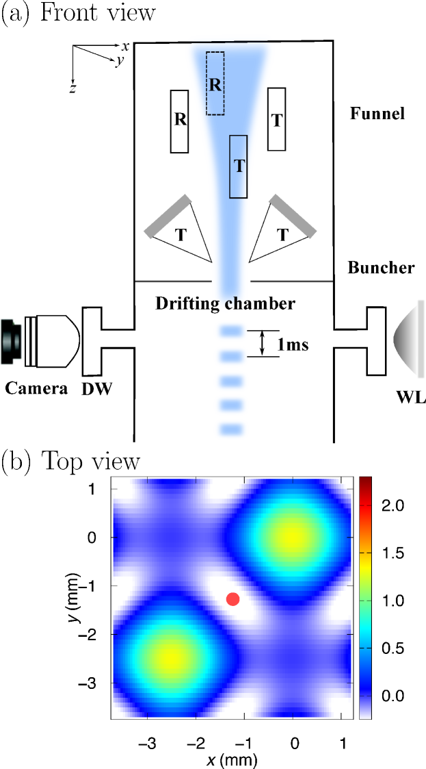
Figure 1: Front view (a), with three-dimensional perspective, of a sketch of the setup, including the configuration of the acoustic funnel and buncher as well as the detection window (DW), which is equipped with white light (WL) illumination and camera. The acoustic funnel is formed by two orthogonal standing wave resonators in the $x,y$ directions, each consisting of a transducer (T) and a reflector (R), and the particle flow is along $z$ direction. A top view of the created acoustic potential is shown in (b). The coordinates refer to the center of the mechanical setup of transducers and reflectors. Potential minima are characterized by an oval shape and the center of one is marked by a red dot at $-(\lambda/4,\lambda/4)$, corresponding to the position where the focusing experiment is performed. Below the funnel, the acoustic buncher is formed by two tilted transducers that emit synchronized acoustic waves. The acoustic wave is transversely focused by a conical cavity with a pinhole Sasaki et al. (2006). The upper chamber is filled with helium gas, at a pressure of $10^{-3}$ mbar, as the acoustic coupling medium. The particle stream enters from the top and moves downward.

As illustrated in Fig. 1, the acoustic funnel is made of two orthogonal half-wavelength cavities formed by transducers and specular reflectors in the transverse direction. The two 1D cavities are set up to overlap in the center of the particle beam. Since the focusing in the transverse $x,y$ directions is similar, we firstly consider the Gor’kov potential $U(x,y;t)$ for focusing in the $x,y$ direction Gor’kov (1961); Oberti et al. (2007); Li et al. (2019)

$$U = \frac{16\pi R^{3}I}{c}\left[\frac{1}{3}f_{1}(\cos^{2}{kx}+\cos^{2}{ky}+2\cos{kx}\cos{ky})\right.$$ (1)

$$\times \left.\sin^{2}{\omega t}-\frac{1}{2}f_{2}(\sin^{2}{kx}+\sin^{2}{ky})\cos^{2}{\omega t}\right]$$

with $f_{1}=1-(\rho{}c^{2})/(\rho_{0}{}c_{0}^{2})$ and $f_{2}=2(\rho_{0}-\rho)/(2\rho_{0}+\rho)$. $I$ and $k$ are the intensity and wave number of the acoustic field, respectively, $R$ is the radius of the particle, $c$ and $\rho$ are the speed of sound in and the density of the coupling medium, and $c_{0}$ and $\rho_{0}$ are the speed of sound in and the density of the particle. Due to the fast velocity of the nanoparticles, we keep the form of Gor’kov force with temporal modulation Gor’kov (1961). As will be shown below, the exact form of static Gor’kov force relies on the condition that the characteristic frequency of particle motion has to be much lower than that of the acoustic wave, such that the particles have stable trajectories, and this condition can be well fulfilled in our scheme.

We assume mass and radius of the particle as $m=3\times{10^{-21}}~{}\text{kg}$ and $R=100$ nm, which resembles typical biological sample particles, such as virus particle. (1) corresponds to the force from the potential of an eigen mode that has a minimum at the center of the cavity $r=0$ Andrade et al. (2015); Barmatz and Collas (1985); Raeymaekers et al. (2011). Assuming the particle has, at least, one symmetry axis and the longitudinal motion is parallel to that axis, there is no deflecting force in the transverse direction Landau and Lifshiftz (1959). Thus the Brownian motion is the dominant mechanism of transverse dispersion of the particle beam. Denoting the transverse velocity as $v_{y}=\dot{y}$, the equation of motion for the Brownian motion in Gor’kov potential is

$$m\dot{v}_{y}+\beta v_{y}=F_{B}(t)+F_{G}(y,t)$$ (2)

$$v_{y}(0)=0\,,y(0)=0\,,$$

where $F_{B}(t)$ is the force of Brownian collision and $F_{G}(y,t)$ is the Gor’kov force. For low pressure, $p\lesssim 10^{-3}$ mbar, helium as the coupling medium, and a Knudsen number close to the transition regime, the friction coefficient $\beta$ can be expressed as

$$\beta=4\pi R^{2}\rho\sqrt{\frac{2k_{B}T}{m_{a}}}\,.$$ (3)

We can linearize the Gor’kov force around $-(\lambda/4,\lambda/4)$ as

$$F_{G}(y,t) = -\frac{16\pi{I}R(kR)^{2}}{c}\left[\left(\frac{1}{3}f_{1}+\frac{1}{2}f_{2}\right)-\cos{2\omega t}\right.$$ (4)

$$\times \left.\left(\frac{1}{3}f_{1}-\frac{1}{2}f_{2}\right)\right]y$$

$$= -Gy\left(1+\frac{H}{G}\cos{2\omega{t}}\right)\,.$$

The motion in the $x$-direction is the same, since the linearized Gor’kov force $F_{G}(x,t)$ can be obtained by replacing $y$ with $x$. The oscillating term in the Gor’kov force that is proportional to $\cos{2\omega{t}}$ can possibly induce parametric resonances and drive particles away from the equilibrium position of the potential. However, it can be shown that the parametric resonance can be safely avoided in our case, due to a large difference between the frequencies of particle oscillation and acoustic wave: Rewriting (LABEL:eq:eom) approximately in the form of a Mathieu equation

$$\ddot{y}+\frac{\beta}{m}\dot{y}+\frac{G}{m}y(1+\frac{H}{G}\cos{2\omega{t}})=0\,.$$ (5)

and denoting $\Omega=\sqrt{{G}/{m}}$ as the characteristic frequency of particle oscillation, the particle trajectory is found as

$$y(t)= e^{-\frac{\beta{t}}{2m}}\left\{C_{1}\mathcal{C}\left[\left(\frac{\Omega}{\omega}\right)^{2}-\left(\frac{\beta}{2m\omega}\right)^{2},-\frac{H}{2G}\left(\frac{\Omega}{\omega}\right)^{2},\omega{t}\right]\right.$$ (6)

$$+\left.C_{2}\mathcal{S}\left[\left(\frac{\Omega}{\omega}\right)^{2}-\left(\frac{\beta}{2m\omega}\right)^{2},-\frac{H}{2G}\left(\frac{\Omega}{\omega}\right)^{2},\omega{t}\right]\right\}\,,$$

where $\mathcal{C}(a,q,\nu)$ and $\mathcal{S}(a,q,\nu)$ are even and odd Mathieu functions.

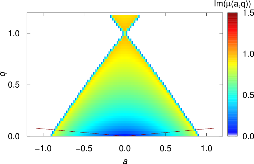
Figure 2: Stability diagram according to (5) with $\beta=0$. The region with a purely imaginary characteristic exponent of ${\rm Im}[\mu(a,q)]>0$ permits stable trajectories according to the Mathieu equation, see color map, and the unstable region is left white. The parameters for our case correspond to the solid lines $a=(\Omega/\omega)^{2}=(2G/H)q$.

Rigorous theory of Mathieu equations gives the stable regime of the particle trajectory with $\beta=0$ Jones (2006); Paul (1990), see Fig. 2. In this parameter space the particles oscillate transversely with limited amplitudes that do not grow exponentially. A wide range of ratios between particle-oscillation and acoustic-wave frequencies provide stable trajectories. The required condition can be conveniently fulfilled even without friction, e. g., in our case $(a,q)\simeq(0.11,4.4\times{10^{-4}})$. Variational analysis demonstrated that the friction can further widen the permitted stable regime according to the Mathieu equation Hsieh (1977, 1980), since it physically suppresses the oscillation amplitude of particle trajectory.

Computations following (5) show converging trajectories to the center of the harmonic potential. In the absence of parametric resonances, the particle trajectories must converge to the focused area. Similar to the case of a pure harmonic potential the temporal factor in the Gor’kov force could be approximately integrated out Gor’kov (1961). Based on the stability analysis, the particle’s velocity is

$$v_{y}(t)=-\frac{\beta}{m}y+\frac{1}{m}\int_{0}^{t}F_{B}(\zeta)d\zeta+\frac{1}{m}F_{G}(y)t\,.$$ (7)

The corresponding Fokker-Planck equation Fokker (1914); Planck (1917); Ornstein (1919) for the transverse distribution of the particles $f(y,y_{0},t)$ can thus be obtained, for the linearized Gor’kov force, as

$$\frac{\partial}{\partial t}f=\frac{G}{\beta}\frac{\partial}{\partial y}(yf)+D\frac{\partial^{2}}{\partial{y}^{2}}f\,.$$ (8)

From the Fokker-Planck equation, the temporal evolution of the transverse particle positions are obtained as

$$f(y,y_{0},t)= \left[\frac{G}{2\pi\beta D(1-e^{-\frac{2G}{\beta}t})}\right]^{1/2}$$ (9)

$$\times\exp\left[-\frac{G}{2{\beta}D}\frac{\left(y-y_{0}e^{-\frac{G}{\beta}t}\right)^{2}}{1-e^{-\frac{2G}{\beta}t}}\right]\,.$$

This yields the minimal width of the particle stream as

$$w_{\text{min}}=\sqrt{\frac{2\ln{2}k_{B}T}{G}}\,.$$ (10)

Given an initial width $w_{0}$, the transverse distribution function $f(y,y_{0},t)$ in (9) can be convoluted as

$$f(y,t) =\int_{-\infty}^{\infty}f(y,y_{0},t)w(y_{0})dy_{0}$$ (11)

$$w(y_{0}) =\sqrt{\frac{\ln 2}{{\pi}w_{0}^{2}}}e^{-\ln 2\,y_{0}^{2}/w_{0}^{2}}\,,$$

which gives the temporal evolution of particle stream

$$f(y,t)= \mathcal{P}\sqrt{\frac{\pi}{{\mathcal{Q}}e^{-\frac{2G}{\beta}t}+\sqrt{\ln{2}/w_{0}^{2}}}}$$ (12)

$$\times\exp\left[-\left(\mathcal{Q}-\frac{\mathcal{Q}^{2}e^{-\frac{2G}{\beta}t}}{{\mathcal{Q}}e^{-\frac{2G}{\beta}t}+\sqrt{\ln{2}/w^{2}_{0}}}\right)y^{2}\right]\,,$$

where $\mathcal{P}(t)=\sqrt{G\ln{2}/(2\pi{}w_{0}^{2}\beta{D}(1-e^{-{2Gt}/{\beta}}))},$ and $\mathcal{Q}(t)=G/(2\beta{D})\cdot 1/(1-e^{-{2Gt}/\beta}).$

The temporal evolution obtained for $w_{0}=100~{}\text{\textmu{m}}$ is presented in Fig. 3. The particle beam is transversely compressed to a width of $6~{}\text{\textmu{m}}$, approaching the size of the XFEL beam. We show the temporal evolution of particle number density distribution determined from (9) in Fig. 3(a), and from numerical simulations in Fig. 3(b) and (c).

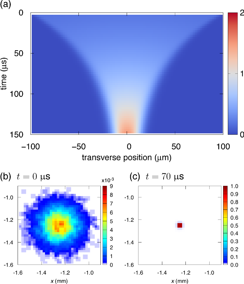
Figure 3: (a) Temporal evolution of a particle distribution with an initial width (waist) $w_{0}=100~{}\text{\textmu{m}}$ in an acoustic wave with frequency $\nu=26$ kHz and an intensity of $I=1~{}\text{W/cm}^{2}\,$. The final width is consistent with the minimal width $w_{\text{min}}=7.5~{}\text{\textmu{m}}$, determined from (10). Particle number density distributions are plotted at (b) 0 µs and (c) 70 µs from numerically simulated dynamics using the 2D potential with explicit time dependence in (1). The root mean squared deviation from the center $(-\lambda/4,-\lambda/4)$ is 100 µm and 6 µm at 0 µs and 70 µs, respectively.

The acoustic buncher relies on the period force imposed by the traveling wave resulting from tilted transducers, see Fig. 1. Suppose the two transducers radiate synchronously with the same phase, then the transverse force is zero and only a force in the longitudinal direction remains. In our case, the particles move with a longitudinal velocity of $v_{z}\sim 100$ m/s, and the buncher imposes a force field that has sufficiently short longitudinal interaction length, i. e., the particle transit time $\Delta{t}=l/v_{z}$ is much shorter than the period of the acoustic wave. Since the acoustic pressure variation does not affect the particle for a full cycle, the particle only experience a transient force. This leads to an acoustic force that is proportional to the first order of the sinusoidal modulation of the plane acoustic wave. Assuming the acoustic pressure to be $p=p_{0}\sin(\vec{k}\cdot\vec{r}-\omega t+\phi_{0})$, it takes a form

$$p=p_{0}\sin\left[\vec{k}\cdot\left(\vec{r}_{0}(t)+\vec{R}\right)-\omega{t}+\phi_{0}\right]\,,$$ (13)

for $\vec{r}=\vec{r}_{0}(t)+\vec{R}$ on the surface of a particle at position $\vec{r}_{0}(t)$ with radius R, where $\vec{k}$ is the wave vector and $\phi_{0}$ is an arbitrary phase. Under this assumption, the acoustic force exerted on the particle is

$$f_{z}= \oiint pdS=\int_{0}^{2\pi}d\phi\int_{0}^{\pi}d\theta\sin\theta R^{2}p_{0}$$ (14)

$$\times\sin\left[kR\cos\theta-\omega{t}+\vec{k}\cdot\vec{r}_{0}(t)+\phi_{0}\right]$$

$$= \frac{4\pi R\sin{kR}}{k}\sin\left(\omega{t}-\vec{k}\cdot\vec{r}_{0}(t)-\phi_{0}\right)\,.$$

Because of the narrow width of the interaction area of the buncher, and the $\lesssim 100$ nm size of the particles, i. e., $kR\ll 1$, the particle scattering effect is suppressed, and the force can be further approximated as $f_{z}\simeq p_{0}S\sin(\omega{t}-\theta_{0})$, where $\theta_{0}$ is a constant phase factor, left to be chosen, and $S$ is the surface area of the particle. In general, we write the effective longitudinal force as $f_{z}=F\sin\omega{t}$.

Considering an acoustic wave with $\nu=1$ kHz and an induced relative pressure variation of $\Delta{}p=2\times 10^{-4}$ mbar, well below the pressure in the chamber, we obtain a force $F=10^{-4}$ pN. The particles experience a periodic velocity modulation with respect to their entrance time into the interaction region of length $d$, yielding $\frac{1}{2}mv^{2}-E_{1}\approx{}Fd\sin\omega{t_{1}}$ with the particle velocity $v_{1}$ and kinetic energy $E_{1}=\frac{1}{2}mv_{1}^{2}$ at the entrance of the interaction region. The length $d$ of the particle-wave-interaction region is chosen such that the particle experiences the force over only $1/10$ of the acoustic wave period. A conical cavity with a pin-hole can focus the acoustic wave to a length on the order of $\lambda/40$ in the near field Sasaki et al. (2006). Considering the wavelength of the 1 kHz acoustic wave, $\lambda=11$ cm, we choose the length of interaction region to be $d=1$ cm, which is experimentally feasible. Thus we have approximately $v=v_{1}\left[1+(Fd/2E_{1})\sin\omega{t_{1}}\right].$

Assuming particles drift for a distance $l$ after leaving the interaction region and arrive at the end of the buncher at time $t_{2}$, we have

$$t_{2}=t_{1}+\frac{l}{v}\simeq t_{1}+\frac{l}{v_{1}}\left(1-\frac{Fd}{2E_{1}}\sin{\omega}t_{1}\right)\,.$$ (15)

With an initial number density $n_{1}$ and the continuity condition $n_{2}dt_{2}=n_{1}dt_{1}$, the modulated number density $n_{2}$ at $t_{2}$ can be expressed as

$$n_{2} =n_{1}+\sum_{k=1}^{\infty}a_{k}\cos\left[k(\omega{t_{2}}-\Theta)\right]+b_{k}\sin\left[k(\omega{t_{2}}-\Theta)\right]$$

with (16)

$$a_{k} =\frac{n_{1}}{\pi}\int_{\Theta-\pi}^{\Theta+\pi}\cos\left[k(\omega{t_{1}}-X\sin{{\omega}t_{1}})\right]d(\omega{t_{1}})$$

$$=2n_{1}J_{k}(kX)$$

$$b_{k} =0\qquad\text{for}\,\,k=1,2,\ldots\,,$$

where $\Theta=l\omega/v_{1}$, $X=Fdl\omega/(2E_{1}v_{1})$, and $J_{k}(x)$ is the Bessel function of $k$-th order. We consider the fundamental harmonic

$$n_{2}=n_{1}+2n_{1}J_{1}(X)\sin({\omega}t_{1}-\Theta)\,.$$ (17)

The degree of bunching is determined by the bunching parameter $X$. The frequency of the traveling wave can be conveniently set as the repetition rate of x-ray pulses.

After the particle stream passes the interaction region of length $d$ it can continue into the next chamber, see Fig. 1, and drifts for a distance $l$ to the interaction point. Assuming $I=1~{}\text{W/cm}^{2}\,$, $\nu=1$ kHz, $d=1$ cm, $v_{1}=100$ m/s, and that the cavities are tilted by $\Psi=\pi/3$, the degree of bunching is maximized as the Bessel function $J_{1}(X)$ reaches its maximum at $X\simeq{1.8}$, which corresponds to a drift length $l=87$ cm.

We numerically simulate the bunching process using particle tracing methods Borland (Advanced Photon Source, 2000).

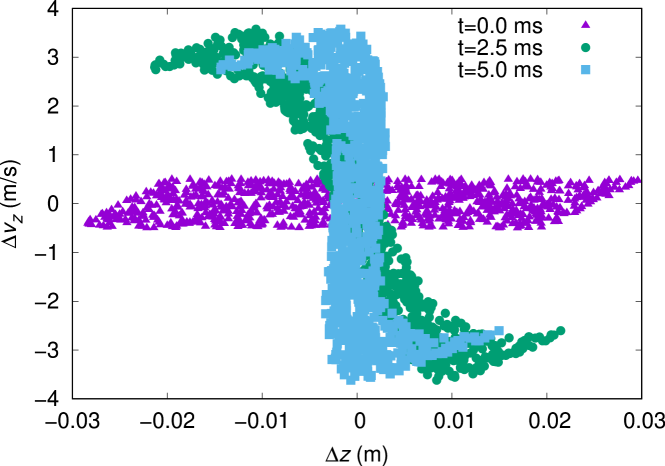
Figure 4: The calculated longitudinal phase-space distribution of the particles is given at the entrance of the buncher, $t=0.0$ ms, and that in the detection region at $t=5.0$ ms as well as an intermediate time $t=2.5$ ms demonstrating the phase-space rotation; all distributions relative to the phase-space position of the synchronous particle.

In the simulation, the buncher is operated such that a 6 cm long packet of molecules with a longitudinal velocity of 100 m/s and a velocity spread of 1 m/s enters the acoustic buncher. The impulse by a force of $10^{-4}$ pN acting on particle of $3\times 10^{-21}$ kg for $\Delta{t}=d/v_{1}{\simeq}0.1$ ms can modulate the velocity by $\Delta{v}\simeq 3.3$ m/s. This can be used as the criterion to choose the acoustic pressure, since the modulation must be similar to that of the velocity spread of the particle beam. The calculated distribution at $t=5$ ms, the time at which the longitudinal spatial focus is obtained downstream of the buncher, is shown in Fig. 4. The longitudinal phase space distribution is relative to the position in phase space of the “synchronous particle” van de Meerakker et al. (2012). In the particular situation depicted in Fig. 4, the molecular packet has a longitudinal focus with a length of about 3 mm some 53 cm after the end of the buncher. The longitudinal focal length is consistent with our simplified model with a single velocity and infinitely short interaction region.

We have proposed an acoustic method to manipulate and compress particle streams by transverse and longitudinal focusing, which enables high-efficiency particle delivery, for instance, for single-particle diffractive imaging experiments with sub-µm-focus x-ray beams. This can substantially reduce the data collection time in such XFEL based imaging experiments. The effective manipulation of particle streams based on acoustic waves could be applied to wider scope of molecular beam experiments, such as matter-wave-interference with large molecules Arndt and Hornberger (2014) as well as applications to fast highly collimated beams Kirian et al. (2015). Furthermore, this work does not just provide an efficient method for acoustic manipulation of gas-phase-particle streams, but also sheds light on the application of the vast particle-optics techniques from accelerator physics to the field of acoustics, e. g., such as particle bunching by the traveling wave from analogues to iris-loaded waveguides.

The authors gratefuly acknowledge stimulating discussions with R. J. Dwayne Miller, Oriol Vendrell, Nikita Medvedev, Sheng Xu, Ludger Inhester, and Henry N. Chapman.

This work has been supported by a Peter Paul Ewald Fellowship of the Volkswagen Foundation, by the European Research Council under the European Union’s Seventh Framework Programme (FP7/2007-2013) through the Consolidator Grant COMOTION (ERC-614507-Küpper), by the Clusters of Excellence “Center for Ultrafast Imaging” (CUI, EXC 1074, ID 194651731) and “Advanced Imaging of Matter” (AIM, EXC 2056, ID 390715994) of the Deutsche Forschungsgemeinschaf, and by the Helmholtz Gemeinschaft through the “Impuls- und Vernetzungsfond”.

References

- Spence and Chapman (2014) John C H Spence and Henry N Chapman, “The birth of a new field,” Phil. Trans. R. Soc. B 369, 20130309–20130309 (2014).
- Hantke et al. (2014) Max F Hantke, Dirk Hasse, Filipe R N C Maia, Tomas Ekeberg, Katja John, Martin Svenda, N Duane Loh, Andrew V Martin, Nicusor Timneanu, Daniel S D Larsson, Gijs van der Schot, Gunilla H Carlsson, Margareta Ingelman, Jakob Andreasson, Daniel Westphal, Mengning Liang, Francesco Stellato, Daniel P Deponte, Robert Hartmann, Nils Kimmel, Richard A Kirian, M Marvin Seibert, Kerstin Mühlig, Sebastian Schorb, Ken Ferguson, Christoph Bostedt, Sebastian Carron, John D Bozek, Daniel Rolles, Artem Rudenko, Sascha Epp, Henry N Chapman, Anton Barty, Janos Hajdu, and Inger Andersson, “High-throughput imaging of heterogeneous cell organelles with an x-ray laser,” Nature Photon. 8, 943–949 (2014).
- Awel et al. (2018) S Awel, R A Kirian, M O Wiedorn, K R Beyerlein, N Roth, D A Horke, D Oberthür, J Knoska, V Mariani, A Morgan, L Adriano, A Tolstikova, P L Xavier, O Yefanov, Andrew Aquila, Anton Barty, S Roy-Chowdhury, M S Hunter, D James, J S Robinson, U Weierstall, A V Rode, S Bajt, Jochen Küpper, and Henry N Chapman, “Femtosecond x-ray diffraction from an aerosolized beam of protein nanocrystals,” J. Appl. Crystallogr. 51, 133–139 (2018).
- Barty et al. (2013) Anton Barty, Jochen Küpper, and Henry N. Chapman, “Molecular imaging using x-ray free-electron lasers,” Ann. Rev. Phys. Chem. 64, 415–435 (2013).
- Kirian et al. (2015) R. A. Kirian, S. Awel, N. Eckerskorn, H. Fleckenstein, M. Wiedorn, L. Adriano, S. Bajt, M. Barthelmess, R. Bean, K. R. Beyerlein, L. M. G. Chavas, M. Domaracky, M. Heymann, D. A. Horke, J. Knoska, M Metz, A Morgan, D Oberthuer, N Roth, T Sato, P L Xavier, O. Yefanov, A. V. Rode, Jochen Küpper, and Henry N. Chapman, “Simple convergent-nozzle aerosol injector for single-particle diffractive imaging with x-ray free-electron lasers,” Struct. Dyn. 2, 041717 (2015).
- Roth et al. (2018) Nils Roth, Salah Awel, Daniel Horke, and Jochen Küpper, “Optimizing aerodynamic lenses for single-particle imaging,” J. Aerosol Sci. 124, 17–29 (2018).
- Horke et al. (2017) Daniel A Horke, Nils Roth, Lena Worbs, and Jochen Küpper, “Characterizing gas flow from aerosol particle injectors,” J. Appl. Phys. 121, 123106 (2017).
- Eckerskorn et al. (2015) Niko Eckerskorn, Richard Bowman, Richard A. Kirian, Salah Awel, Max Wiedorn, Jochen Küpper, Miles J. Padgett, Henry N. Chapman, and Andrei V. Rode, “Optically induced forces imposed in an optical funnel on a stream of particles in air or vacuum,” Phys. Rev. Applied 4, 064001 (2015).
- van de Meerakker et al. (2012) Sebastiaan Y T van de Meerakker, Hendrick L Bethlem, Nicolas Vanhaecke, and Gerard Meijer, “Manipulation and control of molecular beams,” Chem. Rev. 112, 4828–4878 (2012).
- Hadjiconstantinou (2002) N. G. Hadjiconstantinou, “Sound wave propagation in transition-regime micro- and nanochannels,” Phys. Fluids 14, 802 (2002).
- Sasaki et al. (2006) Katsuhiro Sasaki, Morimasa Nishihira, and Kazuhiko Imano, “Low-frequency air-coupled ultrasonic system beyond diffraction limit using pinhole,” Jap. J. Appl. Phys. 45, 4560 (2006).
- Gor’kov (1961) L. P. Gor’kov, “On the forces acting on a small particle in an acoustical field in an ideal fluid,” Doklady Akademii Nauk SSSR 140, 88 (1961).
- Oberti et al. (2007) Stefano Oberti, Adrian Neild, and Jürg Dual, “Manipulation of micrometer sized particles within a micromachined fluidic device to form two-dimensional patterns using ultrasound,” J. Acoust. Soc. Am. 121, 778–785 (2007).
- Li et al. (2019) N. Li, A. Kale, and A. C. Stevenson, “Axial acoustic field barrier for fluidic particle manipulatio,” Appl. Phys. Lett. 114, 013702 (2019).
- Andrade et al. (2015) M. A. B. Andrade, N. Pérez, and J. C. Adamowski, “Particle manipulation by a non-resonant acoustic levitator,” Appl. Phys. Lett. 106, 014101 (2015).
- Barmatz and Collas (1985) M Barmatz and P Collas, “Acoustic radiation potential on a sphere in plane, cylindrical, and spherical standing wave fields,” J. Acoust. Soc. Am. 77, 928–945 (1985).
- Raeymaekers et al. (2011) B. Raeymaekers, C. Pantea, and D. N. Sinha, “Manipulation of diamond nanoparticles using bulk acoustic waves,” J. Appl. Phys. 109, 014317 (2011).
- Landau and Lifshiftz (1959) L. D. Landau and E. M. Lifshiftz, Fluid Mechanics (Pergamon Press, 1959).
- Jones (2006) Timothy Jones, Mathieu equation and the ideal RF-Paul trap (Drexel University, 2006).
- Paul (1990) Wolfgang Paul, “Electromagnetic traps for charged and neutral particles,” Rev. Mod. Phys. 62, 531–540 (1990).
- Hsieh (1977) D. Y. Hsieh, “Variational method and mathieu equation,” J. Math. Phys. 19, 1147 (1977).
- Hsieh (1980) D. Y. Hsieh, “On Mathieu equation with damping,” J. Math. Phys. 21, 722 (1980).
- Fokker (1914) Adriaan Daniël Fokker, “Die mittlere Energie rotierender elektrischer Dipole im Strahlungsfeld,” Ann. Phys. 348, 810–820 (1914).
- Planck (1917) Max Planck, “Über einen Satz der statistischen Dynamik und seine Erweiterung in der Quantentheorie,” Sitzungsber. König. Preuß. Akad. Wiss. Berlin 24, 324–341 (1917).
- Ornstein (1919) L. S. Ornstein, “On Brownian motion,” Proc. Acad. Amst. 21, 96 (1919).
- Borland (Advanced Photon Source, 2000) M. Borland, “elegant: A flexible SDDS- compliant code for accelerator simulation,” Tech. Rep. LS-287 (Advanced Photon Source, 2000).
- Arndt and Hornberger (2014) Markus Arndt and Klaus Hornberger, “Testing the limits of quantum mechanical superpositions,” Nature Phys. 10, 271–277 (2014).