Prethermalization to thermalization crossover in a dilute Bose gas following an interaction ramp

Abstract

The dynamics of a weakly interacting Bose gas at low temperatures is close to integrable due to the approximate quadratic nature of the many-body Hamiltonian. While the short-time physics after an abrupt ramp of the interaction constant is dominated by the integrable dynamics, integrability is broken at longer times by higher-order interaction terms in the Bogoliubov Hamiltonian, in particular by Beliaev-Landau scatterings involving three quasiparticles. The two-stage relaxation process is highlighted in the evolution of local observables such as the density-density correlation function: an integrable dephasing mechanism leads the system to a prethermal stage, followed by true thermalization conveyed by quasiparticle collisions. Our results bring the crossover from prethermalization to thermalization within reach of current experiments with ultracold atomic gases.

I introduction

Ever since the development of quantum mechanics in the early days, it has been a central question how the unitary time evolution of a quantum wavefunction of many particles may generate a seemingly thermal ensemble in the long-time limit – at least in the eyes of an experimenter with limited tools to probe the system. The eigenstate thermalization hypothesis (ETH) Deutsch (1991); Srednicki (1994) aims to address this question by stating that expectation values of macroscopic observables computed with respect to a single generic eigenstate of energy $E$ are the same as the microcanonical average around the corresponding energy. The hypothesis has been verified numerically for a wide series of chaotic quantum systems Rigol et al. (2008); Rigol (2009).

Since it relies on the hypothesis of ergodicity, ETH is not expected to hold for integrable quantum systems. There, an extensive number of conserved quantities restricts the full quantum dynamics to a small subspace of the total phase space, thereby preventing thermalization. The long-time states of integrable systems can still be statistically described by a stationary generalized Gibbs ensemble (GGE) Rigol et al. (2007), that incorporates all the conserved charges, as recently seen in a cold atom experiment Langen et al. (2015). Another seminal experimental example is the quantum Newton cradle Kinoshita et al. (2006). In the same spirit as ETH, a representative eigenstate of the integrable Hamiltonian can be identified based on these conserved charges, which correctly reproduces expectation values of local observables Caux and Essler (2013).

Similarly, approximate integrable systems can go through a dephasing stage, after which they are left in a prethermal state Berges et al. (2004), also described by a GGE with all the approximately conserved quantities. Nevertheless, at longer times true thermalization sets in, conveyed by higher-order relaxation processes, such as illustrated in Fig. 1(a).

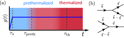
Figure 1: (a) A pictorial image of the separation of time scales considered in this work. The gas is brought out of equilibrium by abruptly ramping up the interaction constant $g$ in a time $\tau_{s}$. Then, the approximate integrability of Hamiltonian (1) leads the system through a prethermalization stage (blue shades) on a time scale $\tau_{\text{preth}}$ set by the chemical potential $\mu$. Finally, a thermal equilibrium is reached on a vastly longer time scale $\tau_{\text{th}}$ through Beliaev-Landau collisions (red shades). Alternatively, the red shades can be seen as representing the growth of thermodynamic entropy. (b) Diagrams of the predominant non-integrable collisions that drive the system toward full thermalization; Beliaev decay (up) and Landau scattering (down).

As of now, the literature on the crossover from a prethermalized to a thermalized state after a global quench has been mostly restricted to toy models. It has been studied how a 1D chain Bertini et al. (2015) or liquid Buchhold et al. (2016) of spinless fermions with weak integrability breaking first relaxes to a prethermal state, after which a kinetic picture allows us to understand the full thermalization dynamics of the model. In this article, we aim to bring the study of the two distinct relaxation mechanisms within the realm of current experiments.

II The Hamiltonian

The weakly interacting Bose gas provides a natural example of an experimentally relevant system that is close to being integrable. It is described by the standard Hamiltonian in 3D (we use units of $\hbar=1$)

$$\hat{H}=\sum_{\mathbf{k}}\frac{k^{2}}{2m}\,\hat{a}^{\dagger}_{\mathbf{k}}\hat{a}_{\mathbf{k}}+\frac{g}{2V}\sum_{\mathbf{p},\mathbf{k},\mathbf{q}}\hat{a}^{\dagger}_{\mathbf{p}+\mathbf{q}}\hat{a}^{\dagger}_{\mathbf{k}-\mathbf{q}}\hat{a}_{\mathbf{k}}\hat{a}_{\mathbf{p}}.$$ (1)

Here, $V$ is the volume of the gas, $m$ is the particle mass and $g$ is the effective interaction constant, found from the $s$-wave scattering length $a_{s}$ as $g=4\pi a_{s}/m$.

Starting from the ground state of an ideal gas with density $n$, we perform an abrupt ramp of the interaction constant $g_{i}\rightarrow g_{f}$ (with $g_{i}=0<g_{f}$) within a nonzero time window $\tau_{s}$ (see Fig. 1(a)), and study the subsequent dynamics under Hamiltonian (1). Experimentally, this can be done with a Feshbach resonance Chin et al. (2010) by suddenly ramping up an external magnetic field. Recently, this mechanism was utilized to probe the analog of cosmic Sakharov oscillations in a 2D bosonic gas Hung et al. (2013). In low dimensions, the interaction constant can also be modified by varying the transverse confinement Jaskula et al. (2012).

When interactions are weak (small $na_{s}^{3}$) and the temperature well below the critical temperature, almost all particles are found in the $\mathbf{k}=0$ mode, justifying the replacement $\hat{a}_{0}\rightarrow\langle\hat{a}_{0}\rangle\equiv\sqrt{n_{0}V}$, where $n_{0}\approx n$ is the condensate density. The dynamics of the bosonic gas after an interaction quench was studied on the level of a quadratic approximation in the fluctuation operators $\hat{a}_{\mathbf{k}}$ ($\mathbf{k}\neq 0$) Natu and Mueller (2013); Carusotto et al. (2010), and later the departure from the prethermalized state was considered Menegoz and Silva (2015) and the damping of the oscillations was added by hand Rançon and Levin (2014).

We, however, seek to explicitly retain terms containing three fluctuation operators as well, so as to describe higher-order (non-integrable) scatterings that eventually lead the system toward thermalization. In the literature on superfluidity, these are commonly studied in the context of Beliaev decay and Landau damping Beliaev (1958), where they are responsible for the damping of a phonon Pitaevskii and Stringari (1997); Giorgini (1998); Chevy et al. (2002); Katz et al. (2002).

By truncating (1) to third order in fluctuation operators, we find the approximate Hamiltonian,

$$\hat{H}\approx E_{0}+\hat{H}_{2}+\hat{H}_{3}.$$ (2)

The quadratic part can be diagonalized with the standard Bogoliubov transformation $\hat{a}_{\mathbf{k}}=u_{k}\hat{\chi}_{\mathbf{k}}+v_{k}\hat{\chi}^{\dagger}_{-\mathbf{k}}$, with

$$u_{k},v_{k}=\pm\sqrt{\frac{k^{2}/2m+gn_{0}}{2\omega_{k}}\pm\frac{1}{2}},$$ (3)

and the quasiparticle frequency

$$\omega_{k}=\sqrt{\frac{k^{2}}{2m}\Big{(}\frac{k^{2}}{2m}+2gn_{0}\Big{)}}.$$ (4)

In terms of the Bogoliubov operators, Hamiltonian (2) is then expressed as Sinatra et al. (2009)

$$\hat{H}_{2} = \sum_{\mathbf{k}}\omega_{k}\hat{\chi}_{\mathbf{k}}^{\dagger}\hat{\chi}_{\mathbf{k}},$$ (5)

$$\hat{H}_{3} = g\sqrt{\frac{n_{0}}{V}}\sum_{\mathbf{k},\mathbf{q}}\Big{(}A_{\mathbf{k},\mathbf{q}}\hat{\chi}_{\mathbf{k}}^{\dagger}\hat{\chi}_{\mathbf{q}}^{\dagger}\hat{\chi}_{\mathbf{k}+\mathbf{q}}+$$ (6)

$$B_{\mathbf{k},\mathbf{q}}\hat{\chi}_{\mathbf{k}}\hat{\chi}_{\mathbf{q}}\hat{\chi}_{-\mathbf{k}-\mathbf{q}}+\text{h.c}\;\Big{)},$$

with the matrix elements of $\hat{H}_{3}$

$$A_{\mathbf{k},\mathbf{q}} = u_{\mathbf{k}}u_{\mathbf{q}}u_{\mathbf{k}+\mathbf{q}}+v_{\mathbf{k}}v_{\mathbf{q}}v_{\mathbf{k}+\mathbf{q}}$$ (7)

$$+\big{(}u_{\mathbf{k}+\mathbf{q}}+v_{\mathbf{k}+\mathbf{q}}\big{)}\big{(}u_{\mathbf{k}}v_{\mathbf{q}}+u_{\mathbf{q}}v_{\mathbf{k}}\big{)},$$

$$B_{\mathbf{k},\mathbf{q}} = \frac{1}{3}(u_{\mathbf{k}}u_{-\mathbf{k}-\mathbf{q}}v_{\mathbf{q}}+(u_{\mathbf{q}}+v_{\mathbf{q}})(u_{\mathbf{k}}v_{-\mathbf{k}-\mathbf{q}}+u_{-\mathbf{k}-\mathbf{q}}v_{\mathbf{k}})$$ (8)

$$+v_{\mathbf{k}}v_{-\mathbf{k}-\mathbf{q}}u_{\mathbf{q}}).$$

Upon taking the thermodynamic limit and rescaling the wave numbers with the healing length after the quench $\xi=\sqrt{1/m\mu}$, $k\to\tilde{k}=k\xi$ one notes that the density of states times the matrix elements of $\hat{H}_{3}$ squared scales as $1/(n\xi^{3})=\sqrt{(4\pi)^{3}na_{s}^{3}}$, exactly like the condensate depletion $n-n_{0}$. Therefore, if the number of depleted particles is sufficiently small, the dynamics under the integrable Hamiltonian $\hat{H}_{2}$ occurs on a substantially faster time scale than the ergodic dynamics of $\hat{H}_{3}$. A similar reasoning to compare third and fourth order terms of the Hamiltonian justifies the omission of $\hat{H}_{4}$ in (2).

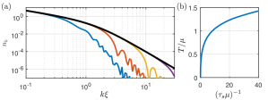
Figure 2: Effect of an interaction quench $g_{i}=0\rightarrow g_{f}$. (a) The momentum distribution $n_{\mathbf{k}}^{(\chi)}$ of quasiparticles after the interaction ramp for decreasing switching times $\tau_{s}=\{5,\;0.5,\;0.05,\;0.005\}\times\mu^{-1}$ from bottom to top; the thick black line is the limiting case $\tau_{s}\rightarrow 0$, for which we have result (13). $n^{(\chi)}_{\mathbf{k}}$ constitutes a conserved charge of $\hat{H}_{2}$ and only evolves under $\hat{H}_{3}$. (b) Upon a decrease in the switching time $\tau_{s}$ more energy is injected into the system, which then translates into a higher equilibrium temperature $T$. For $\tau_{s}\to 0$, we derive $T=O(\tau_{s}^{-1/5})$.

III The equations of motion

We start by looking at the short-time dynamics, generated by $\hat{H}_{2}$, such as studied in Natu and Mueller (2013). In particular, the interaction ramp takes place within a nonzero time window, short enough so that we can safely neglect any effects of $\hat{H}_{3}$ during the quench. We return to the basis of particle operators and find that the dynamics of the quadratic correlation functions $n^{(a)}_{\mathbf{k}}=\langle\hat{a}_{\mathbf{k}}^{\dagger}\hat{a}_{\mathbf{k}}\rangle$ and $c^{(a)}_{\mathbf{k}}=\langle\hat{a}_{\mathbf{k}}\hat{a}_{-\mathbf{k}}\rangle$ is governed by Natu and Mueller (2013)

$$\!\!\!\!\partial_{t}n_{\mathbf{k}}^{(a)} = -2\textrm{Im}\big{[}g(t)n_{0}c^{(a)}_{\mathbf{k}}\big{]},$$ (9)

$$\!\!\!\!i\partial_{t}c_{\mathbf{k}}^{(a)} = 2\Big{(}\frac{k^{2}}{2m}+g(t)n_{0}\Big{)}c_{\mathbf{k}}^{(a)}+g(t)n_{0}(2n_{\mathbf{k}}^{(a)}+1).$$ (10)

This system of equations is readily integrated numerically for a given temporal profile $g(t)$ and with appropriate initial conditions. It has been intensely studied in the context of the dynamical Casimir effect Dodonov (2010), where a modulation of the interaction constant or condensate density causes a change of vacuum for the quasiparticle operators $\hat{\chi}_{\mathbf{k}}$ Jaskula et al. (2012); Carusotto et al. (2010); Koghee and Wouters (2014); Wilson et al. (2011). The correlations of the quasiparticles, in turn, are evaluated with the linear transform

$$n_{\mathbf{k}}^{(\chi)} = \big{(}u_{k}^{2}+v_{k}^{2}\big{)}n_{\mathbf{k}}^{(a)}-2u_{k}v_{k}\textrm{Re}\big{[}c^{(a)}_{\mathbf{k}}\big{]}+v_{k}^{2},$$ (11)

$$c_{\mathbf{k}}^{(\chi)} = u_{k}^{2}c_{\mathbf{k}}^{(a)}+v_{k}^{2}c_{\mathbf{k}}^{(a)\ast}-2u_{k}v_{k}n_{\mathbf{k}}^{(a)}-u_{k}v_{k}.$$ (12)

In the limit of instantaneous switching time $\tau_{s}\rightarrow 0$, $n_{\mathbf{k}}^{(a)}$ and $c_{\mathbf{k}}^{(a)}$ are zero just after the quench and we find the correlation functions after the quench as

$$n_{\mathbf{k}}^{(\chi)}=v^{2}_{k},\;\;\;c_{\mathbf{k}}^{(\chi)}=-u_{k}v_{k}.$$ (13)

In Fig. 2(a), we show the quasiparticle momentum distribution for different $\tau_{s}$ and see that it converges to (13) for shorter $\tau_{s}$.

We now stick to the basis of Bogoliubov operators $\hat{\chi}_{\mathbf{k}}$. Their quadratic correlation functions evolve trivially under $\hat{H}_{2}$ as $n_{\mathbf{k}}^{(\chi)}(t)=n_{\mathbf{k}}^{(\chi)}$ and $c_{\mathbf{k}}^{(\chi)}(t)=\tilde{c}_{\mathbf{k}}^{(\chi)}e^{-2i\omega_{k}t}$, making $n_{\mathbf{k}}^{(\chi)}$ and $\tilde{c}_{\mathbf{k}}^{(\chi)}$ conserved quantities of $\hat{H}_{2}$ related to the integrable dynamics. However, they do experience a variation under the full Hamiltonian (2), which breaks the integrability. Via Heisenberg’s equation of motion, we derive their dynamics under $\hat{H}_{3}$:

$$\partial_{t}n_{\mathbf{k}}^{(\chi)} = 2g\sqrt{\frac{n_{0}}{V}}\textrm{Im}\bigg{\{}\sum_{\mathbf{q}}3B_{\mathbf{k},-\mathbf{q}}R^{\ast}_{\mathbf{k},\mathbf{q}}$$ (14)

$$+2A_{\mathbf{k},\mathbf{q}-\mathbf{k}}M_{\mathbf{q},\mathbf{k}}+A_{\mathbf{q},\mathbf{k}-\mathbf{q}}M^{\ast}_{\mathbf{k},\mathbf{q}}\bigg{\}}$$

$$i\partial_{t}\tilde{c}_{\mathbf{k}}^{(\chi)} = 2g\sqrt{\frac{n_{0}}{V}}\sum_{\mathbf{q}}\bigg{\{}3B_{-\mathbf{k},\mathbf{q}}M_{\mathbf{k},\mathbf{q}}$$ (15)

$$+2A_{\mathbf{k},-\mathbf{q}}M^{\ast}_{\mathbf{q},\mathbf{k}}+A_{\mathbf{q},\mathbf{k}-\mathbf{q}}R_{\mathbf{k},\mathbf{q}}\bigg{\}}e^{2i\omega_{k}t},$$

where we have introduced the correlation functions of three quasiparticles

$$M_{\mathbf{k},\mathbf{q}}=\Big{\langle}\hat{\chi}^{\dagger}_{\mathbf{k}-\mathbf{q}}\hat{\chi}^{\dagger}_{\mathbf{q}}\hat{\chi}_{\mathbf{k}}\Big{\rangle},\;\;\;R_{\mathbf{k},\mathbf{q}}=\Big{\langle}\hat{\chi}_{\mathbf{q}-\mathbf{k}}\hat{\chi}_{-\mathbf{q}}\hat{\chi}_{\mathbf{k}}\Big{\rangle}.$$ (16)

We next evaluate the equation of motion for these third-order correlators

$$i\partial_{t}M_{\mathbf{k},\mathbf{q}} = (\omega_{\mathbf{k}}-\omega_{\mathbf{q}}-\omega_{\mathbf{k}-\mathbf{q}})M_{\mathbf{k},\mathbf{q}}+g\sqrt{\frac{n_{0}}{V}}F^{(M)}_{\mathbf{k},\mathbf{q}},$$ (17)

$$i\partial_{t}R_{\mathbf{k},\mathbf{q}} = (\omega_{\mathbf{k}}+\omega_{\mathbf{q}}+\omega_{\mathbf{q}-\mathbf{k}})R_{\mathbf{k},\mathbf{q}}+g\sqrt{\frac{n_{0}}{V}}F^{(R)}_{\mathbf{k},\mathbf{q}}.$$ (18)

Here, the matrices $F^{(M,R)}_{\mathbf{k},\mathbf{q}}$ contain correlators of four operators. More generally, a connected correlator of $p$ operators couples to correlators of $p+1$ operators on the right-hand side, making this an ever-growing hierarchy Proukakis (2001). However, as explained in Van Regemortel et al. (2017), fourth-order correlators in $F^{(M,R)}_{\mathbf{k},\mathbf{q}}$ can be approximately factorized into products of second-order correlators using Wick’s theorem, thus establishing a truncated hierarchy of correlations functions. After this factorization, we find the drive term in Eqs. (17)–(18) as (we drop the superscript ${\boldsymbol{\cdot}}^{(\chi)}$ for ease of notation)

$$F^{(M)}_{\mathbf{k},\mathbf{q}} = 2A_{\mathbf{k},-\mathbf{q}}\Big{(}c^{\ast}_{\mathbf{q}}(n_{\mathbf{k}-\mathbf{q}}-n_{\mathbf{k}})-c^{\ast}_{\mathbf{k}-\mathbf{q}}c_{\mathbf{k}}\Big{)}$$ (19)

$$+2A_{\mathbf{k},\mathbf{q}-\mathbf{k}}\Big{(}c^{\ast}_{\mathbf{k}-\mathbf{q}}(n_{\mathbf{q}}-n_{\mathbf{k}})-c_{\mathbf{k}}c^{\ast}_{\mathbf{q}}\Big{)}$$

$$+2A_{\mathbf{q},\mathbf{k}-\mathbf{q}}\Big{(}n_{\mathbf{k}-\mathbf{q}}(n_{\mathbf{q}}-n_{\mathbf{k}})-n_{\mathbf{k}}(n_{\mathbf{q}}+1)\Big{)}$$

$$+3B_{\mathbf{k},-\mathbf{q}}\Big{(}c^{\ast}_{\mathbf{k}-\mathbf{q}}c^{\ast}_{\mathbf{q}}-c_{\mathbf{k}}n_{\mathbf{k}-\mathbf{q}}\Big{)}$$

$$+3B_{\mathbf{k},\mathbf{q}-\mathbf{k}}\Big{(}c^{\ast}_{\mathbf{k}-\mathbf{q}}c^{\ast}_{\mathbf{q}}-c_{\mathbf{k}}(n_{\mathbf{q}}+1)\Big{)}$$

$$-3B_{\mathbf{q},\mathbf{k}-\mathbf{q}}\;c_{\mathbf{k}}\Big{(}n_{\mathbf{q}}+n_{\mathbf{k}-\mathbf{q}}+1\Big{)},$$

and

$$F^{(R)}_{\mathbf{k},\mathbf{q}} = 2A_{\mathbf{k},-\mathbf{q}}\Big{(}c_{\mathbf{k}-\mathbf{q}}(n_{\mathbf{k}}+n_{\mathbf{q}}+1)+c_{\mathbf{k}}c_{\mathbf{q}}\Big{)}$$ (20)

$$+2A_{\mathbf{k},\mathbf{q}-\mathbf{k}}\Big{(}c_{\mathbf{q}}(n_{\mathbf{k}}+n_{\mathbf{k}-\mathbf{q}}+1)+c_{\mathbf{k}-\mathbf{q}}c_{\mathbf{k}}\Big{)}$$

$$+2A_{\mathbf{q},\mathbf{k}-\mathbf{q}}\Big{(}c_{\mathbf{k}}(n_{\mathbf{q}}+n_{\mathbf{k}-\mathbf{q}}+1)+c_{\mathbf{q}}c_{\mathbf{k}-\mathbf{q}}\Big{)}$$

$$+3B_{\mathbf{k},-\mathbf{q}}\;\Big{(}(n_{\mathbf{k}-\mathbf{q}}+1)(n_{\mathbf{k}}+n_{\mathbf{q}}+1)\Big{)}$$

$$+3B_{\mathbf{k},\mathbf{q}-\mathbf{k}}\Big{(}n_{\mathbf{q}}(n_{\mathbf{k}}+n_{\mathbf{k}-\mathbf{q}}+1)+n_{\mathbf{k}-\mathbf{q}}+1\Big{)}$$

$$+3B_{\mathbf{q},\mathbf{k}-\mathbf{q}}\;\Big{(}n_{\mathbf{k}}(n_{\mathbf{q}}+n_{\mathbf{k}-\mathbf{q}}+1)\Big{)}.$$

As such, we establish a closed set of differential equations for correlators up to order three, which approximately describes the dynamics of the bosonic gas after the interaction ramp, provided $n_{0}\gg n-n_{0}$, ensuring that connected correlators of higher order have a decreasing magnitude.

IV The kinetic equations

In the long-time limit, the coupled system of equations (14)–(15) and (17)–(18) reproduces the well-known kinetic equations. This can be seen by formally solving (17) as

$$M_{\mathbf{k},\mathbf{q}}(t)=-ig\sqrt{\frac{n_{0}}{V}}\int_{0}^{t}ds\;F_{\mathbf{k},\mathbf{q}}^{(M)}(s)\;e^{i(\omega_{\mathbf{k}}-\omega_{\mathbf{q}}-\omega_{\mathbf{k}-\mathbf{q}})(s-t)},$$ (21)

and similar for $R_{\mathbf{k},\mathbf{q}}(t)$ in (18). These expressions can now be plugged into (14)–(15), after which we obtain effective dynamics by $(i)$ sending the integration boundary $t\rightarrow\infty$ in (21), thus singling out non-oscillating terms in the integral over $s$, and $(ii)$ time averaging Eq. (14) to remove the contributions that oscillate rapidly with time $t$. The result is that the evolution of quasiparticle occupation numbers is governed by the kinetic (or quantum Boltzmann) equations

$$\partial_{t}n_{\mathbf{k}} = 4\pi\frac{g^{2}n_{0}}{V}\bigg{\{}\sum_{\mathbf{q}}A^{2}_{\mathbf{q},\mathbf{k}-\mathbf{q}}\delta\big{(}\omega_{\mathbf{k}}-\omega_{\mathbf{q}}-\omega_{\mathbf{k}-\mathbf{q}}\big{)}$$ (22)

$$\;\;\;\times\Big{(}n_{\mathbf{k}-\mathbf{q}}n_{\mathbf{q}}-n_{\mathbf{k}}(n_{\mathbf{q}}+n_{\mathbf{k}-\mathbf{q}}+1)\Big{)}$$

$$+2\sum_{\mathbf{q}}A^{2}_{\mathbf{k},\mathbf{q}-\mathbf{k}}\delta\big{(}\omega_{\mathbf{q}}-\omega_{\mathbf{k}}-\omega_{{\mathbf{q}-\mathbf{k}}}\big{)}$$

$$\;\;\;\times\Big{(}n_{\mathbf{q}}(n_{\mathbf{k}}+n_{{\mathbf{q}-\mathbf{k}}}+1)-n_{\mathbf{k}}n_{{\mathbf{q}-\mathbf{k}}}\Big{)}\bigg{\}}.$$

Within the kinetic approximation, the oscillation frequencies from the evolution of $M_{\mathbf{k},\mathbf{q}}$ have been translated into $\delta$-functions imposing energy conservation for the redistribution of quasiparticle occupation numbers. In our method, the kinetic equations come as a limiting behavior, so that deviations from them can be studied quantitatively, as we do in Fig. 3; this to our knowledge has not been done previously in 3D.

With (22), we rederive the kinetic equation that is known from the literature on Beliaev-Landau scattering, where it is commonly established with Fermi’s golden rule Sinatra et al. (2009). The first term represents the redistribution of quasiparticles through Beliaev decay, where a quasiparticle with high momentum $\mathbf{k}$ decays into (or is formed from) two with $\mathbf{q}$ and $\mathbf{k}-\mathbf{q}$. The second term, in turn, describes the Landau process of absorption (or emission) of the quasiparticle with momentum $\mathbf{k}$ by a quasiparticle $\mathbf{q}-\mathbf{k}$ (or $\mathbf{q}$). Notice that the Landau term comes with an additional factor $2$ from the two possible scattering channels Giorgini (1998). See Fig. 1(b) for the corresponding diagrams.

Through the same analysis, we obtain the evolution of pair correlations,

$$i\partial_{t}{c}_{\mathbf{k}}=\left(2\omega_{\textbf{k}}+2\delta\omega_{\textbf{k}}-i{\gamma_{\textbf{k}}}\right){c}_{\mathbf{k}}+I_{\textbf{k}}(\{c_{\textbf{q}}\})$$ (23)

The first term ur this equation contains the evolution of ${c}_{\mathbf{k}}$ under the Bogoliubov frequency $z_{\textbf{k}}=\omega_{\textbf{k}}+\delta\omega_{\textbf{k}}-i{\gamma_{\textbf{k}}}/2$ calculated treating $\hat{H}_{3}$ in second order perturbation theory in the instantaneous Fock state $|n_{\textbf{k}},\{n_{\textbf{q}}\}_{\textbf{q}\neq\textbf{k}}\rangle$ (see the Appendix for the explicit derivation). This contains the Landau-Beliaev damping rate

$$\gamma_{\mathbf{k}}=4\pi\frac{g^{2}n_{0}}{V}\sum_{\textbf{q}}\left[A^{2}_{\mathbf{q},\mathbf{k}-\mathbf{q}}(n_{\mathbf{q}}+n_{\mathbf{k}-\mathbf{q}}+1)\delta\big{(}\omega_{\mathbf{k}}-\omega_{\mathbf{q}}-\omega_{\mathbf{k}-\mathbf{q}}\big{)}+2A^{2}_{\mathbf{k},\mathbf{q}-\mathbf{k}}(n_{\mathbf{q}-\mathbf{k}}-n_{\mathbf{q}})\delta\big{(}\omega_{\mathbf{q}}-\omega_{\mathbf{k}}-\omega_{\mathbf{q}-\mathbf{k}}\big{)},\right]$$ (24)

(where the Beliaev and Landau parts are respectively the first and second summation) and the frequency shift

$$\delta\omega_{\mathbf{k}}=\frac{g^{2}n_{0}}{V}\mathcal{P}\sum_{\textbf{q}}\Bigg{[}\frac{2A^{2}_{\mathbf{q},\mathbf{k}-\mathbf{q}}(n_{\mathbf{q}}+n_{\mathbf{k}-\mathbf{q}}+1)}{\omega_{\mathbf{k}}-\omega_{\mathbf{q}}-\omega_{\mathbf{k}-\mathbf{q}}}+\frac{4A^{2}_{\mathbf{k},\mathbf{q}-\mathbf{k}}(n_{\mathbf{q}-\mathbf{k}}-n_{\mathbf{q}})}{\omega_{\mathbf{k}}+\omega_{\mathbf{q}-\mathbf{k}}-\omega_{\mathbf{q}}}-\frac{18B^{2}_{\mathbf{k},\mathbf{q}}(n_{\mathbf{q}}+n_{-\mathbf{k}-\mathbf{q}}+1)}{\omega_{\mathbf{k}}+\omega_{\mathbf{q}}+\omega_{-\mathbf{k}-\mathbf{q}}}\Bigg{]},$$ (25)

where $\mathcal{P}$ denotes the Cauchy principal value and we have used the fact that our momentum distribution remains symmetric $n_{\textbf{k}}^{(\chi)}=n_{-\textbf{k}}^{(\chi)}$. The collisional integral $I_{\textbf{k}}(\{c_{\textbf{q}}\})$ accounts for the fact that the distribution $\{c_{\textbf{q}}\}$ in modes $\textbf{q}\neq\textbf{k}$ changes dynamically with $c_{\textbf{k}}$; it is given by

$$I_{\textbf{k}}(\{c_{\textbf{q}}\})=2\frac{g^{2}n_{0}}{V}\Bigg{[}\sum_{\mathbf{q}}\frac{2A^{2}_{\mathbf{q},\mathbf{k}-\mathbf{q}}{c}_{\mathbf{q}}{c}_{\mathbf{k}-\mathbf{q}}}{\omega_{\textbf{q}}+\omega_{\textbf{k}-\textbf{q}}-\omega_{\textbf{k}}+i0^{+}}+\frac{4A^{2}_{\mathbf{k},\mathbf{q}-\mathbf{k}}{c}_{\mathbf{q}}{c}^{\ast}_{\mathbf{q}-\mathbf{k}}}{\omega_{\textbf{q}}-\omega_{\textbf{k}}-\omega_{\textbf{q}-\textbf{k}}+i0^{+}}+\frac{18B_{\textbf{k},\textbf{q}}^{2}\tilde{c}_{\mathbf{-\textbf{k}-\textbf{q}}}^{*}\tilde{c}_{\mathbf{\textbf{q}}}^{*}}{-\omega_{\textbf{k}}-\omega_{\textbf{q}}-\omega_{-\textbf{k}-\textbf{q}}+i0^{+}}\Bigg{]},$$ (26)

Eq. (23) describes how the coherence between modes k and $-\textbf{k}$ evolves under three-body scatterings, and in particular $I_{\textbf{k}}$ describes how it is affected by the coherence in other modes q. Remark that $c_{\textbf{k}}$ may show a temporal evolution even if the populations $n_{\textbf{k}}$ are prepared at thermal equilibrium, reflecting the underlying Landau-Beliaev scatterings that maintain equilibrium. To our knowledge, this equation was not found in the literature, unlike the kinetic equation (22) on $n_{\textbf{k}}$ Lipschitz and Pitaevskii (1981).

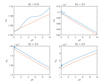
Figure 3: A comparison of the quasiparticle occupation numbers $n_{\mathbf{k}}$ as produced by the integration of the hierarchy of correlation functions (blue lines) and the derived kinetic equation in the adiabatic limit (red lines) for the quench $g_{i}=0\rightarrow g_{f}=0.05\mu\xi^{3}$ (corresponding to $n\xi^{3}=20$) in $\tau_{s}=0.5\mu^{-1}$ for different momenta (see the initial momentum distribution of quasi-particles right after the quench on Fig. 2).

In Fig. 3, we perform a quantitative comparison between the full integration of the truncated hierarchy and the approximate kinetic description (22). We show the evolution of the quasiparticle occupation numbers at short times $t\sim 1/\mu$. We observe that the curve of $n_{k}(t)$ predicted by the kinetic equation differs in two distinct ways from that of the hierarchy: $(i)$ the evolution at very short times is not well captured by the kinetic equation, which results in a small offset (controlled by the interaction strength $na_{s}^{3}$) between the two curves, an offset then conserved all along the evolution and $(ii)$ contrary to the kinetic description, the hierarchy of correlations retains high-frequency components in $n_{k}(t)$. Those two differences are directly related to the approximations $(i)$ and $(ii)$ detailed in the main text below (21), on which kinetic equations are based.

In the long-time limit, we find that (22) and (23) converge to the values in a thermal ensemble. The momentum distribution of quasiparticles approaches the Bose-Einstein distribution

$$n^{\text{th}}_{\mathbf{k}}=\frac{1}{e^{\beta\omega_{\mathbf{k}}}-1},$$ (27)

with $\beta=1/k_{B}T$ the inverse temperature set by the total injected energy, while the anomalous correlations vanish. The energy after the quench on the level of the quadratic Hamiltonian, $E=E_{0}+\sum_{\mathbf{k}}\omega_{k}\,n^{(\chi)}_{k}$, is conserved under the kinetic equations. However, using the value of the mode occupation number $n^{(\chi)}_{k}$ for an infinitely fast quench [see Eq. (13)] leads to an ultraviolet divergence of this injected energy. This divergence is regularized by a finite switching time: this sets an effective cutoff in energy $\omega_{k_{\rm max}}\propto 1/\tau_{s}$, corresponding to a momentum cutoff $k_{\rm max}\propto 1/\sqrt{\tau_{s}}$ in the limit of fast quench $\tau_{s}\to 0$, and therefore to an injected energy $E-E_{0}\propto 1/\sqrt{\tau_{s}}$. This enables us to fix the total injected energy with the switching time $\tau_{s}$ and, consequently, the final equilibrium temperature of the gas by matching this energy with the energy of a thermal ensemble. When $k_{B}T>\mu$, we have that $E-E_{0}\propto T^{5/2}$ , such that we derive the asymptotic scaling $T\propto\tau_{s}^{-1/5}$. In Fig. 2(b), we show the full variation of equilibrium temperature with switching time $\tau_{s}$.

V The density-density correlation function

Finally, we investigate the behavior of macroscopic observables in real space, which are expected to exhibit the two distinct relaxation stages. We concentrate on distances of the order of the (equilibrium) thermal wavelength $2\pi/k_{\text{th}}$, with $\omega_{k_{\text{th}}}=k_{B}T$. We choose $\tau_{s}^{-1}=0.5\mu$, such that $k_{B}T=0.67\mu$ and therefore the thermal wavelength is of the same order as the healing length $\xi$. For $k\sim 1/\xi$, the kinetic equations are accurate for times $t>1/\mu$, and introduce an offset of the order of $\sqrt{na_{\rm s}^{3}}$, our small parameter. Therefore, they correctly describe the dynamics of spatial correlations at length scales $\sim\xi$ in the weakly interacting limit, as we have also checked numerically.

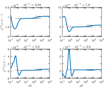
Figure 4: The evolution of the density correlation function after the quench $g_{i}=0\rightarrow g_{f}=0.05\mu\xi^{3}$ in $\tau_{s}=0.5\mu^{-1}$ for varying distances $x=|\mathbf{r}-\mathbf{r}^{\prime}|$ according to the kinetic picture Eqs. (22) and (23). The horizontal solid lines indicate the asymptotic values for the prethermal and thermal (quasi)stationary ensemble; the temperature $T=0.67\mu$ is found from the initial state. At short distances, we clearly notice a relaxation to a prethermal plateau on a time scale of the order of $\tau_{\text{preth}}=\mu^{-1}$ (for ramps $\tau_{s}\sim\mu^{-1}$ and $x\sim\xi$), this is due to a dephasing mechanism in $\hat{H}_{2}$. In $g^{(2)}(x;t)$, this is manifested as a fast oscillation at short times, which then diminishes due to a destructive interference between all $\mathbf{k}$-modes once the light-cone correlation peak has moved away from the considered distance $x$ Carusotto et al. (2010). Then, at much later times, $\tau_{\text{therm}}\sim 10^{3}\mu^{-1}$, a new equilibrium value is found that corresponds to the value in the thermal ensemble through the much slower dynamics of $\hat{H}_{3}$. The difference between the prethermal and thermal value vanishes for increasing separation $x$ as the correlation function drops to zero in this limit.

The first relaxation stage of local observables to their prethermal value is caused by a dephasing mechanism where all $\mathbf{k}$-modes interfere desructively. We therefore define the annihilation operator in position space $\hat{a}(\mathbf{r})=1/\sqrt{V}\sum_{\mathbf{k}}e^{i\mathbf{k}\cdot\mathbf{r}}\hat{a}_{\mathbf{k}}$. Our analysis is now focused on the evolution of the density-density correlation function, defined as $g^{(2)}(\mathbf{r}-\mathbf{r}^{\prime};t)=\langle:\hat{n}(\mathbf{r})\,\hat{n}(\mathbf{r}^{\prime}):\rangle_{t}/\langle\hat{n}(\mathbf{r})\rangle_{t}^{2}$ for a homogeneously distributed gas, where ‘$:$’ denotes normal ordering and $\hat{n}(\mathbf{r})=\hat{a}^{\dagger}(\mathbf{r})\hat{a}(\mathbf{r})$ is the local density operator. The density-density correlation function has proven its importance previously in the context of analog gravity Balbinot et al. (2008); Carusotto et al. (2008), where the correlation pattern shows a fingerprint of the analog of Hawking radiation at an acoustic black hole’s horizon Steinhauer (2016).

On the Gaussian level, the density correlation function can be simplified to

$$g^{(2)}(\mathbf{r}-\mathbf{r}^{\prime};t)=1+\frac{2}{n_{0}}\big{(}\mathfrak{n}(\mathbf{r}-\mathbf{r}^{\prime};t)+\text{Re}\big{\{}\mathfrak{m}(\mathbf{r}-\mathbf{r}^{\prime};t)\big{\}}\big{)},$$ (28)

where we defined

$$\mathfrak{n}(\mathbf{r}-\mathbf{r}^{\prime};t)=\langle\hat{a}^{\dagger}(\mathbf{r})\hat{a}(\mathbf{r}^{\prime})\rangle_{t}=\frac{1}{V}\sum_{\mathbf{k}\neq 0}e^{i\mathbf{k}\cdot(\mathbf{r}-\mathbf{r}^{\prime})}n_{\mathbf{k}}^{(a)}(t),$$ (29)

and analogous for $\mathfrak{m}(\mathbf{r}-\mathbf{r}^{\prime})=\langle\hat{a}(\mathbf{r})\hat{a}(\mathbf{r}^{\prime})\rangle$. The quadratic correlations of fluctuations, $n_{\mathbf{k}}^{(a)}$ and $c_{\mathbf{k}}^{(a)}$, can be obtained from the quasiparticle correlations $n_{\mathbf{k}}^{(\chi)}$ and $c_{\mathbf{k}}^{(\chi)}$ through the inverse of the transformation (11)–(12).

In Fig. 4 we show the evolution of the density correlation function after a ramp $g_{i}=0\rightarrow g_{f}=0.05\mu\xi^{3}$ (so that $na^{3}_{s}=1.3\cdot 10^{-5}$) at different distances $x=|\mathbf{r}-\mathbf{r}^{\prime}|$. We observe a clear first relaxation, approximately to the prethermal value on a time scale $\tau_{\text{preth}}\sim\mu^{-1}$ after an initial oscillation due to the light-cone peak Calabrese and Cardy (2005); Carusotto et al. (2010) that dies out due to dephasing once this has traveled away; this is governed by $\hat{H}_{2}$. At much longer times, the scatterings contained in $\hat{H}_{3}$ cause a new relaxation, this time to the thermal value. We find that the thermalization time $\tau_{\text{therm}}\sim 10^{3}\mu^{-1}$ is in qualitative agreement with the Beliaev-Landau lifetime of the thermal wavenumber $1/\gamma^{BL}_{k_{\text{th}}}\sim 1/\mu\sqrt{na_{s}^{3}}$ for $k_{B}T\sim\mu$ Sinatra et al. (2009).

VI Conclusions

We have illustrated that the crossover from a prethermalized to a thermalized state can be witnessed in a cold atomic gas by probing the density correlations after a sudden interaction ramp. The switching time of the ramp determines the final temperature in the equilibrium ensemble. While a simple dephasing mechanism, treated on the level of the (integrable) quadratic Hamiltonian, causes local observables to relax to a prethermal value, a more sophisticated approach is needed to describe the thermalization stage. Here, third-order interaction processes, known as Beliaev-Landau collisions, are the predominant mechanism to lead the system away from integrability and, eventually, to thermal equilibrium. When focusing on most relevant length scales of the order of the equilibrium thermal wavelength, a kinetic description is sufficient to describe the final relaxation. In principle, our predictions are within reach of current experiments with ultracold atomic gases.

Appendix: Perturbed Bogoliubov energy in an arbitrary excited state

To recover Eqs. (24–25), we treat $\hat{H}_{3}$ as a perturbation of $\hat{H}_{2}$ and we recall Cohen-Tannoudji et al. (1988); Kurkjian et al. (2017) that the complex poles $E$ of the resolvent (or equivalently of the Green function) in a given state $|\psi\rangle$ are given to second order in the perturbation by

$$E = E_{0}+\langle\psi|\hat{H}_{3}|\psi\rangle+\langle\psi|\hat{H}_{3}\frac{\hat{Q}}{E-\hat{H}_{2}}\hat{H}_{3}|\psi\rangle$$ (30)

$$= E_{0}+\langle\psi|\hat{H}_{3}|\psi\rangle+\sum_{\lambda}\frac{|\langle\psi|\hat{H}_{3}|\lambda\rangle|^{2}}{E-\langle\lambda|\hat{H}_{2}|\lambda\rangle}$$ (31)

where $E_{0}=\langle\psi|\hat{H}_{2}|\psi\rangle$ is the unperturbed energy, $\hat{Q}=1-|\psi\rangle\langle\psi|$ projects orthogonally to $|\psi\rangle$ and the states $|\lambda\rangle$ are therefore orthogonal to $|\psi\rangle$. We apply Eq. (31) to the Fock states $|n_{\textbf{k}},\{n_{\textbf{q}}\}_{\textbf{q}\neq\textbf{k}}\rangle$ and $|n_{\textbf{k}}-1,\{n_{\textbf{q}}\}_{\textbf{q}\neq\textbf{k}}\rangle$ whose perturbed energies, respectively $E(n_{\textbf{k}})$ and $E(n_{\textbf{k}}-1)$, define the perturbed Bogoliubov frequency

$$z_{\textbf{k}}\equiv E(n_{\textbf{k}})-E(n_{\textbf{k}}-1)$$ (32)

Changing the sum over the intermediate Fock states $\lambda$ into a sum over the scattered momentum q (taking care to avoid double countings) and replacing in the denominator $E(n_{\textbf{k}})$ by its zeroth-order approximation $E_{0}(n_{\textbf{k}})$ we get

$$\!\!\!\!\!\!z_{\textbf{k}}\!=\!z_{\textbf{k},0}\\ +g^{2}\frac{n_{0}}{V}\sum_{\textbf{q}}\!\Bigg{[}\!\frac{2A_{\textbf{q},\textbf{k}-\textbf{q}}^{2}[(1+n_{\textbf{k}-\textbf{q}})(1+n_{\textbf{q}})-n_{\textbf{k}-\textbf{q}}n_{\textbf{q}}]}{z_{\textbf{k},0}-\omega_{\textbf{q}}-\omega_{\textbf{k}-\textbf{q}}}\\ +\frac{4A_{\textbf{k},\textbf{q}-\textbf{k}}^{2}[(1+n_{\textbf{q}})n_{\textbf{q}-\textbf{k}}-n_{\textbf{q}}(1+n_{\textbf{q}-\textbf{k}})]}{z_{\textbf{k},0}+\omega_{\textbf{q}-\textbf{k}}-\omega_{\textbf{q}}}\\ +\frac{18B_{\textbf{k},\textbf{q}}^{2}[n_{-\textbf{k}-\textbf{q}}n_{\textbf{q}}-(1+n_{-\textbf{k}-\textbf{q}})(1+n_{\textbf{q}})]}{z_{\textbf{k},0}+\omega_{\textbf{q}}+\omega_{-\textbf{k}-\textbf{q}}}\Bigg{]}$$ (33)

where $z_{\textbf{k},0}=E_{0}(n_{\textbf{k}})-E_{0}(n_{\textbf{k}}-1)=\omega_{\textbf{k}}+i0^{+}$ is the unperturbed Bogoliubov frequency. The counting factors originate in our symmetric writing (6) of $\hat{H}_{3}$ where the same operator appears more than once. Using the Plemelj formula $1/(x+i0^{+})=\mathcal{P}(1/x)-i\pi\delta(x)$ to split the real and imaginary parts finally yields Eqs. (24–25).

References

• Deutsch (1991) J. M. Deutsch, Physical Review A 43, 2046 (1991).
• Srednicki (1994) M. Srednicki, Physical Review E 50, 888 (1994).
• Rigol et al. (2008) M. Rigol, V. Dunjko,  and M. Olshanii, Nature 452, 854 (2008).
• Rigol (2009) M. Rigol, Physical Review A 80, 053607 (2009).
• Rigol et al. (2007) M. Rigol, V. Dunjko, V. Yurovsky,  and M. Olshanii, Physical review letters 98, 050405 (2007).
• Langen et al. (2015) T. Langen, S. Erne, R. Geiger, B. Rauer, T. Schweigler, M. Kuhnert, W. Rohringer, I. E. Mazets, T. Gasenzer,  and J. Schmiedmayer, Science 348, 207 (2015).
• Kinoshita et al. (2006) T. Kinoshita, T. Wenger,  and D. S. Weiss, Nature 440, 900 (2006).
• Caux and Essler (2013) J.-S. Caux and F. H. Essler, Physical review letters 110, 257203 (2013).
• Berges et al. (2004) J. Berges, S. Borsányi,  and C. Wetterich, Phys. Rev. Lett. 93, 142002 (2004).
• Bertini et al. (2015) B. Bertini, F. H. Essler, S. Groha,  and N. J. Robinson, Physical review letters 115, 180601 (2015).
• Buchhold et al. (2016) M. Buchhold, M. Heyl,  and S. Diehl, Phys. Rev. A 94, 013601 (2016).
• Chin et al. (2010) C. Chin, R. Grimm, P. Julienne,  and E. Tiesinga, Reviews of Modern Physics 82, 1225 (2010).
• Hung et al. (2013) C.-L. Hung, V. Gurarie,  and C. Chin, Science , 1237557 (2013).
• Jaskula et al. (2012) J.-C. Jaskula, G. B. Partridge, M. Bonneau, R. Lopes, J. Ruaudel, D. Boiron,  and C. I. Westbrook, Phys. Rev. Lett. 109, 220401 (2012).
• Castin and Dum (1998) Y. Castin and R. Dum, Physical Review A 57, 3008 (1998).
• Sinatra et al. (2009) A. Sinatra, Y. Castin,  and E. Witkowska, Physical Review A 80, 033614 (2009).
• Natu and Mueller (2013) S. S. Natu and E. J. Mueller, Physical Review A 87, 053607 (2013).
• Carusotto et al. (2010) I. Carusotto, R. Balbinot, A. Fabbri,  and A. Recati, The European Physical Journal D 56, 391 (2010).
• Menegoz and Silva (2015) G. Menegoz and A. Silva, Journal of Statistical Mechanics: Theory and Experiment 2015, P05035 (2015).
• Rançon and Levin (2014) A. Rançon and K. Levin, Physical Review A 90, 021602 (2014).
• Beliaev (1958) S. Beliaev, Sov. Phys. JETP 34, 299 (1958).
• Pitaevskii and Stringari (1997) L. Pitaevskii and S. Stringari, Physics Letters A 235, 398 (1997).
• Giorgini (1998) S. Giorgini, Physical Review A 57, 2949 (1998).
• Chevy et al. (2002) F. Chevy, V. Bretin, P. Rosenbusch, K. W. Madison,  and J. Dalibard, Phys. Rev. Lett. 88, 250402 (2002).
• Katz et al. (2002) N. Katz, J. Steinhauer, R. Ozeri,  and N. Davidson, Physical review letters 89, 220401 (2002).
• Dodonov (2010) V. Dodonov, Physica Scripta 82, 038105 (2010).
• Koghee and Wouters (2014) S. Koghee and M. Wouters, Physical review letters 112, 036406 (2014).
• Wilson et al. (2011) C. Wilson, G. Johansson, A. Pourkabirian, M. Simoen, J. Johansson, T. Duty, F. Nori,  and P. Delsing, Nature 479, 376 (2011).
• Proukakis (2001) N. P. Proukakis, Journal of Physics B: Atomic, Molecular and Optical Physics 34, 4737 (2001).
• Van Regemortel et al. (2017) M. Van Regemortel, W. Casteels, I. Carusotto,  and M. Wouters, Phys. Rev. A 96, 053854 (2017).
• Lipschitz and Pitaevskii (1981) E. Lipschitz and L. Pitaevskii, in Landau and Lifshitz Course of Theoretical Physics, Vol. 10 (Pergamon Press, New York, 1981) Chap. VII.
• Balbinot et al. (2008) R. Balbinot, A. Fabbri, S. Fagnocchi, A. Recati,  and I. Carusotto, Physical Review A 78, 021603 (2008).
• Carusotto et al. (2008) I. Carusotto, S. Fagnocchi, A. Recati, R. Balbinot,  and A. Fabbri, New Journal of Physics 10, 103001 (2008).
• Steinhauer (2016) J. Steinhauer, Nature Physics 12, 959 (2016).
• Calabrese and Cardy (2005) P. Calabrese and J. Cardy, Journal of Statistical Mechanics: Theory and Experiment 2005, P04010 (2005).
• Cohen-Tannoudji et al. (1988) C. Cohen-Tannoudji, J. Dupont-Roc,  and G. Grynberg, Processus d’interaction entre photons et atomes (InterEditions et Éditions du CNRS, Paris, 1988).
• Kurkjian et al. (2017) H. Kurkjian, Y. Castin,  and A. Sinatra, Annalen der Physik 529, 1600352 (2017).