MLtuner: System Support for Automatic Machine Learning Tuning

Abstract

MLtuner automatically tunes settings for training tunables—such as the learning rate, the momentum, the mini-batch size, and the data staleness bound—that have a significant impact on large-scale machine learning (ML) performance. Traditionally, these tunables are set manually, which is unsurprisingly error prone and difficult to do without extensive domain knowledge. MLtuner uses efficient snapshotting, branching, and optimization-guided online trial-and-error to find good initial settings as well as to re-tune settings during execution. Experiments show that MLtuner can robustly find and re-tune tunable settings for a variety of ML applications, including image classification (for 3 models and 2 datasets), video classification, and matrix factorization. Compared to state-of-the-art ML auto-tuning approaches, MLtuner is more robust for large problems and over an order of magnitude faster.

1 Introduction

Large-scale machine learning (ML) is quickly becoming a common activity for many organizations. ML training computations generally use iterative algorithms to converge on thousands to millions of parameter values that make a pre-chosen model (e.g., a neural network or pair of factor matrices) statistically approximate the reality corresponding to the input training data over which they iterate. Trained models can be used to predict, cluster, or otherwise help explain subsequent data.

For training of large, complex models, parallel execution over multiple cluster nodes is warranted. The algorithms and frameworks used generally have multiple tunables that have significant impact on the execution and convergence rates. For example, the learning rate is a key tunable when using stochastic gradient descent (SGD) for training. As another example, the data staleness bound is a key tunable when using frameworks that explicitly balance asynchrony benefits with inconsistency costs lazytable ; muli-ps .

These tunables are usually manually configured or left to broad defaults. Unfortunately, knowing the right settings is often quite challenging. The best tunable settings can depend on the chosen model, model hyperparameters (e.g., number and types of layers in a neural network), the algorithm, the framework, and the resources on which the ML application executes. As a result, manual approaches not surprisingly involve considerable effort by domain experts or yield (often highly) suboptimal training times and solution quality. Our interactions with both experienced and novice ML users comport with this characterization.

MLtuner is a tool for automatically tuning ML application training tunables. It hooks into and guides a training system in trying different settings. MLtuner determines initial tunable settings based on rapid trial-and-error search, wherein each option tested runs for a small (automatically determined) amount of time, to find good settings based on the convergence rate. It repeats this process when convergence slows, to see if different settings provide faster convergence and/or better solution. This paper describes MLtuner’s design and how it addresses challenges in auto-tuning ML applications, such as large search spaces, noisy convergence progress, variations in effective trial times, best tunable settings changing over time, when to re-tune, etc.

We have integrated MLtuner with two different state-of-the-art training systems and experimented with several real ML applications, including a recommendation application on a CPU-based parameter server system and both image classification and video classification on a GPU-based parameter server system. For increased breadth, we also experimented with three different popular models and two datasets for image classification. The results show MLtuner’s effectiveness: MLtuner consistently zeroes in on good tunables, in each case, guiding training to match and exceed the best settings we have found for the given application/model/dataset. Comparing to state-of-the-art hyperparameter tuning approaches, such as Spearmint spearmint and Hyperband hyperband , MLtuner completes over an order of magnitude faster and does not exhibit the same robustness issues for large models/datasets.

This paper makes the following primary contributions. First, it introduces the first approach for automatically tuning the multiple tunables associated with an ML application within the context of a single execution of that application. Second, it describes a tool (MLtuner) that implements the approach, overcoming various challenges, and how MLtuner was integrated with two different ML training systems. Third, it presents results from experiments with real ML applications, including several models and datasets, demonstrating the efficacy of this new approach in removing the “black art” of tuning from ML application training without the orders of magnitude runtime increases of existing auto-tuning approaches.

2 Background and related work

2.1 Distributed machine learning

The goal of an ML task is to train the model parameters of an ML model on a set of training data, so that the trained model can be used to make predictions on unseen data. The fitness error of the model parameters to the training data is defined as the training loss, computed from an objective function. The ML task often minimizes the objective function (thus the training loss) with an iterative convergent algorithm, such as stochastic gradient descent (SGD). The model parameters are first initialized randomly, and in every step, the SGD algorithm samples one mini-batch of the training data and computes the gradients of the objective function, w.r.t. the model parameters. The parameter updates will be the opposite direction of the gradients, multiplied by a learning rate.

To speed up ML tasks, users often distribute the ML computations with a data parallel approach, where the training data is partitioned across multiple ML workers. Each ML worker keeps a local copy of the model parameters and computes parameter updates based on its training data and local parameter copy. The ML workers propagate their parameter updates and refresh their local parameter copies with the updates every clock, which is often logically defined as some quantity of work (e.g., every training data batch). Data parallel training is often achieved with a parameter server system muli-ps ; geeps ; bosen ; iterstore ; projectadam ; dean2012large ; yahoolda ; piccolo , which manages a global version of the parameter data and aggregates the parameter updates from the workers.

2.2 Machine learning tunables

ML training often requires the selection and tuning of many training hyperparameters. For example, the SGD algorithm has a learning rate (a.k.a. step size) hyperparameter that controls the magnitude of the model parameter updates. The training batch size hyperparameter controls the size of the training data mini-batch that each worker processes each clock. Many deep learning applications use the momentum technique sutskever2013importance with SGD, which exhibit a momentum hyperparameter, to smooth updates across different training batches. In data-parallel training, ML workers can have temporarily inconsistent parameter copies, and in order to guarantee model convergence, consistency models (such as SSP ssp ; lazytable or bounded staleness muli-ps ) are often used, which provide tunable data staleness bounds.

Many practitioners (as well as our own experiments) have found that the settings of the training hyperparameters have a big impact on the completion time of an ML task (e.g., orders of magnitude slower with bad settings)  senior2013empirical ; ngiam2011optimization ; adagrad ; adarevision ; adadelta ; adam ; ssp ; lazytable and even the quality of the converged model (e.g., lower classification accuracy with bad settings)  senior2013empirical ; ngiam2011optimization . To emphasize that training hyperparameters need to be tuned, we call them training tunables in this paper.

The training tunables should be distinguished from another class of ML hyperparameters, called model hyperparameters. The training tunables control the training procedure but do not change the model (i.e., they are not in the objective function), whereas the model hyperparameters define the model and appear in the objective function. Example model hyperparameters include model type (e.g., logistic regression or SVM), neural network depth and width, and regularization method and magnitude. MLtuner focuses on improving the efficiency of training tunable tuning, and could potentially be used to select training tunables in an inner loop of existing approaches that tune model hyperparameters.

2.3 Related work on machine learning tuning

2.3.1 Manual tuning by domain experts

The most common tuning approach is to do it manually (e.g., inception-v3 ; inception-bn ; googlenet ; alexnet ; resnet ; poseidon ). Practitioners often either use some uilt-in defaults or pick training tunable settings via trial-and-error. Manual tuning is inefficient, and the tunable settings chosen are often suboptimal.

For some tasks, such as training a deep neural network for image classification, practitioners find it is important to decrease the learning rate during training in order to get a model with good classification accuracy inception-v3 ; inception-bn ; googlenet ; alexnet ; resnet ; poseidon , and there are typically two approaches of doing that. The first approach (taken by alexnet ; poseidon ) is to manually change the learning rate when the classification accuracy plateaus (i.e., stops increasing), which requires considerable user efforts for monitoring the training. The second approach (taken by inception-v3 ; inception-bn ; googlenet ) is to decay the learning rate $\eta$ over time $t$, with a function of $\eta=\eta_{0}\times\gamma^{t}$. The learning rate decaying factor $\gamma$, as a training tunable, is even harder to tune than the learning rate, because it affects the future learning rate. To decide the best $\gamma$ setting for a training task, practitioners often need to train the model to completion several times, with different $\gamma$ settings.

2.3.2 Traditional hyperparameter tuning approaches

There is prior work on automatic ML hyperparameter tuning (sometimes also called model search), including spearmint ; hyperband ; tupaq ; vartaksupporting ; bergstra2013making ; komer2014hyperopt ; bergstra2011algorithms ; maclaurin2015gradient ; pedregosa2016hyperparameter ; feurer2015efficient ; thornton2013auto . However, none of the prior work distinguishes training tunables from model hyperparameters; instead, they tune both of them together in a combined search space. Because many of their design choices are made for model hyperparameter tuning, we find them inefficient and insufficient for training tunable tuning.

To find good model hyperparameters, many traditional tuning approaches train models from initialization to completion with different hyperparameter settings and pick the model with the best quality (e.g., in terms of its cross-validation accuracy for a classification task). The hyperparameter settings to be evaluated are often decided with bandit optimization algorithms, such as Bayesian optimization movckus1975bayesian or HyperOpt hyperopt . Some tuning approaches, such as Hyperband hyperband and TuPAQ tupaq , reduce the tuning cost by stopping the lower-performing settings early, based on the model qualities achieved in the early stage of training.

MLtuner differs from existing approaches in several ways. First, MLtuner trains the model to completion only once, with the automatically decided best tunable settings, because training tunables do not change the model, whereas existing approaches train multiple models to completion multiple times, incurring considerable tuning cost. Second, MLtuner uses training loss, rather than cross-validation model qualities, as the feedback to evaluate tunable settings. Training loss can be obtained for every training batch at no extra cost, because SGD-based training algorithms use training loss to compute parameter updates, whereas the model quality is evaluated by testing the model on validation data, and the associated cost does not allow it to be frequently evaluated (often every thousands of training batches). Hence, MLtuner can use more frequent feedback to find good tunable settings in less time than traditional approaches. This option is enabled by the fact that, unlike model hyperparameters, training tunables do not change the mathematical formula of the objective function, so just comparing the training loss is sufficient. Third, MLtuner automatically decides the amount of resource (i.e., training time) to use for evaluating each tunable setting, based on the noisiness of the training loss, while existing approaches either hard-code the trial effort (e.g., TuPAQ always uses 10 iterations) or decide it via a grid search (e.g., Hyperband iterates over each of the possible resource allocation plans). Fourth, MLtuner is able to re-tune tunables during training, while existing approaches use the same hyperparameter setting for the whole training. Unlike model hyperparameters, training tunables can (and often should) be dynamically changed during training, as discussed above.

2.3.3 Adaptive SGD learning rate tuning algorithms

Because the SGD algorithm is well-known for being sensitive to the learning rate (LR) setting, experts have designed many adaptive SGD learning rate tuning algorithms, including AdaRevision adarevision , RMSProp rmsprop , Nesterov nesterov , Adam adam , AdaDelta adadelta , and AdaGrad adagrad . These algorithms adaptively adjust the LR for individual model parameters based on the magnitude of their gradients. For example, they often use relatively large LRs for parameters with small gradients and relatively small LRs for parameters with large gradients. However, these algorithms still require users to set the initial LR. Even though they are less sensitive to the initial LR settings than the original SGD algorithm, our experiment results in Section 5.3 show that bad initial LR settings can cause the training time to be orders of magnitude longer (e.g., Figure 7) and/or cause the model to converge to suboptimal solutions (e.g., Figure 6). Hence, MLtuner complements these adaptive LR algorithms, in that users can use MLtuner to pick the initial LR for more robust performance. Moreover, practitioners also find that sometimes using these adaptive LR tuning algorithms alone is not enough to achieve the optimal model solution, especially for complex models such as deep neural networks. For example, Szegedy et al. inception-v3 reported that they used LR decaying together with RMSProp to train their Inception-v3 model.

3 MLtuner: more efficient automatic tuning

This section describes the high level design of our MLtuner approach.

3.1 MLtuner overview

MLtuner automatically tunes training tunables with low overhead, and will dynamically re-tune tunables during the training. MLtuner is a light-weight system that can be connected to existing training systems, such as a parameter server. MLtuner sends the tunable setting trial instructions to the training system and receives training feedback (e.g., per-clock training losses) from the training system. The detailed training system interfaces will be described in Section 4.5. Similar to the other hyperparameter tuning approaches, such as Spearmint spearmint , Hyperband hyperband , and TuPAQ tupaq , MLtuner requires users to specify the tunables to be tuned, with the type—either discrete, continuous in linear scale, or continuous in log scale—and range of valid values.

3.2 Trying and evaluating tunable settings

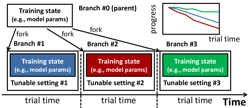
Figure 1: Trying tunable settings in training branches. The red branch with tunable setting #2 has the fastest convergence speed.

MLtuner evaluates tunable settings by trying them in forked training branches. The training branches are forked from the same consistent snapshot of some initial training state (e.g., model parameters, worker-local state, and training data), but are assigned with different tunable settings to train the model. As is illustrated in Figure 1, MLtuner schedules each training branch to run for some automatically decided amount of trial time, and collects their training progress to measure their convergence speed. MLtuner will fork multiple branches to try different settings, and then pick only the branch with the fastest convergence speed to keep training, and kill the other branches. In our example applications, such as deep learning and matrix factorization, the training system reports the per-clock training losses to MLtuner as the training progress.

The training branches are scheduled by MLtuner in a time-sharing manner, running in the same training system instance on the same set of machines. We made this design choice, rather than running multiple training branches in parallel on different sets of machines, for three reasons. First, this design avoids the use of extra machines that are just for the trials; otherwise, the extra machines will be wasted when the trials are not running (which is most of the time). Second, this design allows us to use the same hardware setup (e.g., number of machines) for both the tuning and the actual training; otherwise, the setting found on a different hardware setup would be suboptimal for the actual training. Third, running all branches in the same training system instance helps us achieve low overhead for forking and switching between branches, which are now simply memory copying of training state within the same process and choosing the right copy to use. Also, some resources, such as cache memory and immutable training data, can be shared among branches without duplication.

3.3 Tunable tuning procedure

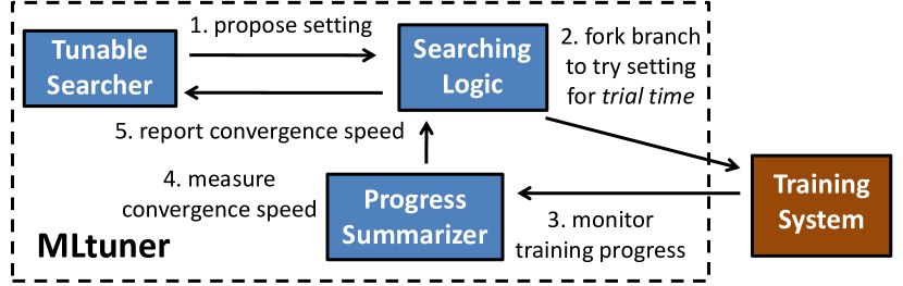
Figure 2: MLtuner tuning procedure.

Figure 2 illustrates the tuning procedure of MLtuner. MLtuner first tags the current training state as the parent branch. Then, inside the tuning loop, MLtuner uses a tunable searcher module (described in Section 4.3) to decide the next tunable setting to evaluate. For each proposed trial setting, MLtuner will instruct the training system to fork a trial branch from the parent branch to train the model for some amount of trial time with the trial setting. Section 4.2 will describe how MLtuner automatically decides the trial time. Then, MLtuner will collect the training progress of the trial branch from the training system, and use the progress summarizer module (described in Section 4.1) to summarize its convergence speed. The convergence speed will be reported back to the tunable searcher to guide its future tunable setting proposals. MLtuner uses this tuning procedure to tune tunables at the beginning of the training, as well as to re-tune tunables during training. Re-tuning will be described in Section 4.4.

3.4 Assumptions and limitations

The design of MLtuner relies on the assumption that the good tunable settings (in terms of completion time and converged model quality) can be decided based on their convergence speeds measured with a relatively short period of trial time. The same assumption has also been made by many of the state-of-the-art hyperparameter tuning approaches. For example, both Hyperband and TuPAQ stop some of the trial hyperparameter settings early, based on the model qualities achieved in the early stage of the training. This assumption does not always hold for model hyperparameter tuning. For example, a more complex model often takes more time to converge but will eventually converge to a better solution. For most of the training tunables, we find this assumption holds for all the applications that we have experimented with so far, including image classification on two different datasets with three different deep neural networks, video classification, and matrix factorization. That is because the training tunables only control the training procedure but do not change the model. That is also the reason why we do not suggest using MLtuner to tune the model hyperparameters. For use cases where both training tunables and model hyperparameters need to be tuned, users can use MLtuner in the inner loop to tune the training tunables, and use the existing model hyperparameter tuning approaches in the outer loop to tune the model hyperparameters.

4 MLtuner implementation details

This section describes the design and implementation details of MLtuner.

4.1 Measuring convergence speed

The progress summarizer module takes in the training progress trace (e.g., a series of training loss) of each trial branch, and outputs the convergence speed. The progress trace has the form of $\{(t_{i},x_{i})\}_{i=1}^{N}$, where $t_{i}$ is the timestamp, and $x_{i}$ is the progress. In this section, we assume $x$ is the training loss, and a smaller $x$ value means better convergence.

Downsampling the progress trace. The most straightforward way of measuring the convergence speed is to use the slope of the progress trace: $s=\frac{|x_{N}-x_{1}|}{t_{N}-t_{1}}$. However, in many ML applications, such as deep neural network training with SGD, the progress trace is often quite noisy, because the training loss points are computed on different batches of the training data. We find the convergence speed measured with just the first and last point of the progress trace is often inaccurate. To deal with the noisiness, the progress summarizer will downsample the progress trace of each branch, by uniformly dividing the progress trace into $K$ non-overlapping windows. The value of each window will be calculated as the average of all data points in it. For a downsampled progress trace of $\{(\tilde{t}_{i},\tilde{x}_{i})\}_{i=1}^{K}$, its slope will be $\tilde{s}=\frac{-range(\tilde{x})}{range(\tilde{t})}$, where $range(\tilde{x})=\tilde{x}_{K}-\tilde{x}_{1}$ and $range(\tilde{t})=\tilde{t}_{K}-\tilde{t}_{1}$. We will describe how we decide $K$ later in this section.

Penalizing unstable branches. Even with downsampling, calculating the slope by simply looking at the first and last downsampled points might still treat branches with unstable jumpy loss as good converging branches. To deal with this problem, the summarizer module will adjust the convergence speed estimation of each branch according to its noisiness. Ideally, the loss of a noise-free trace $\tilde{x}^{(nf)}$ should be monotonically decreasing, so we estimate the noisiness of a trace $\tilde{x}$ as $noise(\tilde{x})=\max{(\max\limits_{1\leq i\leq K-1}{(\tilde{x}_{i+1}-\tilde{x}_{i})},0)}$, which is the maximum magnitude that a point goes up from the previous point. In order to make a conservative estimation of convergence speeds, our progress summarizer will penalize the convergence speed of each branch with its noise:
$speed=\max{(\frac{-range(\tilde{x})-noise(\tilde{x})}{range(\tilde{t})},0)}$. which is a positive value for a converging branch and zero for a diverged branch. We report zero as the convergence speed of a diverged branch, rather than reporting it as a negative value, because we find it is usually wrong to treat a diverged branch with smaller diverged loss as a better branch than other diverged branches. We treat diverged branches as of the same quality.

Convergence and stability checks. The progress summarizer will check the convergence and stability of each branch, and assign one of the three labels to them: converging, diverged, or unstable. It labels a branch as converging, if $range(\tilde{x})<0$ and $noise(\tilde{x})<\epsilon\times|range(\tilde{x})|$. We will describe how we decide $\epsilon$ later in this section. It labels a branch as diverged, if the training encounters numerically overflowed numbers. Finally, it labels all the other branches as unstable, meaning that their convergence speeds might need longer trials to evaluate. With a longer trial time, an unstable branch might become stable, because its $|range(\tilde{x})|$ is likely to increase because of the longer training, and its $noise(\tilde{x})$ is likely to decrease because of more points being averaged in each downsampling window.

Deciding number of samples and stability threshold. The previously described progress summarizer module has two knobs, the number of samples $K$ and the stability threshold $\epsilon$. Since the goal of MLtuner is to free users from tuning, $K$ and $\epsilon$ do not need to be tuned by users either. To decide $K$, we will consider an extreme case, where the true convergence progress $|range(\tilde{x}^{(nf)})|$ is zero, and $\tilde{x}$ is all white noise, following a normal distribution. This trace will be falsely labelled as converging, if $\{\tilde{x}_{i}\}_{i=1}^{K}$ is monotonically decreasing, and this probability is less than ${(\frac{1}{2})}^{K}$. Hence, we need a large enough $K$ to bound this false positive probability. We decide to set $K=10$ to counter the noisiness, so that the false positive probability is less than 0.1%. The $\epsilon$ configuration bounds the magnitude (relative to $|range(\tilde{x})|$) that each point in the progress trace is allowed to go up from the previous point. On average, if we approximate the noise-free progress trace $\tilde{x}^{(nf)}$ as a straight line, each point is expected to go down from the previous point by $\approx\frac{|range(\tilde{x})|}{K}$. Hence, MLtuner sets $\epsilon$ to $\frac{1}{K}$, so that a converging trace will have no point going up by more than it is expected to go down. Our experiments in Section 5 show that the same settings of $K$ and $\epsilon$ work robustly for all of our application benchmarks.

4.2 Deciding tunable trial time

Unlike traditional tuning approaches, MLtuner automatically decides tunable trial time, based on the noisiness of training progress, so that the trial time is just long enough for good tunable settings to have stable converging progress. Algorithm 1 illustrates the trial time decision procedure. MLtuner first initializes the trial time to a small value, such as making it as long as the decision time of the tunable searcher, so that the decision time will not dominate. While MLtuner tries tunable settings, if none of the settings tried so far is labelled as converging with the current trial time, MLtuner will double the trial time and use the doubled trial time to try new settings as well as the previously tried settings for longer. When MLtuner successfully finds a stable converging setting, the trial time is decided and will be used to evaluate future settings.

Algorithm 1 MLtuner trial time decision.

$trialTime\leftarrow 0$

Parent branch $\leftarrow$ current model state

while none of the settings is converging do

    Get $tunableSetting$ from tunable searcher

    $trialTime\leftarrow\max(trialTime,searcherDecisionTime)$

    if $tunableSetting$ is not empty then

        Fork a branch from the parent branch with $tunableSetting$

        Append the new branch to $trialBranches$

    end if

    for each $branch$ in $trialBranches$ do

        Schedule $branch$ to run for $trialTime-branch.runTime$

    end for

    Summarize the progress of all $trialBranches$

    Remove diverged branches from $trialBranches$

    if any $branch$ in $trialBranches$ is converging then

        $bestSetting\leftarrow$ tunable setting that has the best convergence

        Free the non-best branches

        Trial time decided and break out the loop

    else

        $trialTime\leftarrow trialTime\times 2$

    end if

end while

Keep searching with $trialTime$

4.3 Tunable searcher

The tunable searcher is a replaceable module that searches for a best tunable setting that maximizes the convergence speed. It can be modeled as a black-box function optimization problem (i.e., bandit optimization), where the function input is a tunable setting, and the function output is the achieved convergence speed. MLtuner allows users to choose from a variety of optimization algorithms, with a general tunable searcher interface. In our current implementation, we have implemented and explored four types of searchers, including RandomSearcher, GridSearcher, BayesianOptSearcher, and HyperOptSearcher.

The simplest RandomSearcher just samples settings uniformly from the search space, without considering the convergence speeds of previous trials. GridSearcher is similar to RandomSearcher, except that it discretizes the continuous search space into a grid, and proposes each of the discretized settings in the grid. Despite its simplicity, we find GridSearcher works surprisingly well for low-dimensional cases, such as when there is only one tunable to be searched. For high-dimensional cases, where there are many tunables to be searched, we find it is better to use bandit optimization algorithms, which spend more searching efforts on the more promising part of the search space. Our BayesianOptSearcher uses the Bayesian optimization algorithm, implemented in the Spearmint spearmint package, and our HyperOptSearcher uses the HyperOpt hyperopt algorithm. Through our experiments, we find HyperOptSearcher works best among all the searcher choices for most use cases, and MLtuner uses it as its default searcher.

The tunable searcher (except for GridSearcher) need a stopping condition to decide when to stop searching. Generally, it can just use the default stopping condition that comes with the optimization packages. Unfortunately, neither the Spearmint nor HyperOpt package provides a stopping condition. They all rely on users to decide when to stop. After discussing with many experienced ML practitioners, we used a rule-of-thumb stopping condition for hyperparameter optimization, which is to stop searching when the top five best (non-zero) convergence speeds differ by less than 10%.

4.4 Re-tuning tunables during training

MLtuner re-tunes tunables, when the training stops making further converging progress (i.e., considered as converged) with the current tunable setting. We have also explored designs that re-tune tunables more aggressively, before the converging progress stops, but we did not choose those designs for two reasons. First, we find the cost of re-tuning usually outweighs the increased convergence rate coming from the re-tuned setting. Second, we find, for some complex deep neural network models, re-tuning too aggressively might cause them to converge to suboptimal local minimas.

To re-tune, the most straightforward approach is to use exactly the same tuning procedure as is used for initial tuning, which was our initial design. However, some practical issues were found, when we deployed it in practice. For example, re-tuning happens when the training stops making converging progress, but, if the training has indeed converged to the optimal solution and no further converging progress can be achieved with any tunable setting, the original tuning procedure will be stuck in the searching loop for ever.

To address this problem, we find it is necessary to bound both the per-setting trial time and the number of trials to be performed for each re-tuning. For the deep learning applications used in Section 5, MLtuner will bound the per-setting trial time to be at most one epoch (i.e., one whole pass over the training data), and we find, in practice, this bound usually will not be reached, unless the model has indeed converged. MLtuner also bounds the number of tunable trials of each re-tuning to be no more than the number of trials of the previous re-tuning. The intuition is that, as more re-tunings are performed, the likelihood that a better setting is yet to be found decreases. These two bounds together will guarantee that the searching procedure can successfully stop for a converged model.

4.5 Training system interface

Method name	Input	Description
Messages sent from MLtuner
ForkBranch	(clock, branchId, parentBranchId, tunable[, type])	fork a branch by taking a consistent snapshot at clock
FreeBranch	(clock, branchId)	free a branch at clock
ScheduleBranch	(clock, branchId)	schedule the branch to run at clock
Messages sent to MLtuner
ReportProgress	(clock, progress)	report per-clock training progress

Table 1: MLtuner message signatures.

MLtuner works as a separate process that communicates with the training system via messages. Table 1 lists the message signatures. MLtuner identifies each branch with a unique branch ID, and uses clock to indicate logical time. The clock is unique and totally ordered across all branches. When MLtuner forks a branch, it expects the training system to create a new training branch by taking a consistent snapshot of all state (e.g., model parameters) from the parent branch and use the provided tunable setting for the new branch. When MLtuner frees a branch, the training system can then reclaim all the resources (e.g., memory for model parameters) associated with that branch. MLtuner sends the branch operations in clock order, and it sends exactly one ScheduleBranch message for every clock. The training system is expected to report its training progress with the ReportProgress message every clock.

Although in our MLtuner design, the branches are scheduled based on time, rather than clocks, our MLtuner implementation actually sends the per-clock branch schedules to the training system. We made this implementation choice, in order to ease the modification of the training systems. To make sure that a trial branch runs for (approximately) the amount of scheduled trial time, MLtuner will first schedule that branch to run for some small number of clocks (e.g., three) to measure its per-clock time, and then schedule it to run for more clocks, based on the measured per-clock time. Also, because MLtuner consumes very few CPU cycles and little network bandwidth, users do not need to dedicate a separate machine for it. Instead, users can just run MLtuner on one of the training machines.

Distributed training support. Large-scale machine learning tasks are often trained with distributed training systems (e.g., with a parameter server architecture). For a distributed training system with multiple training workers, MLtuner will broadcast the branch operations to all the training workers, with the operations in the same order. MLtuner also allows each of the training workers to report their training progress separately, and MLtuner will aggregate the training progress with a user-defined aggregation function. For all the SGD-based applications in this paper, where the training progress is the loss computed as the sum of the training loss from all the workers, this aggregation function just does the sum.

Evaluating the model on validation set. For some applications, such as the classification tasks, the model quality (e.g., classification accuracy) is often periodically evaluated on a set of validation data during the training. This can be easily achieved with the branching support of MLtuner. To test the model, MLtuner will fork a branch with a special TESTING flag as the branch type, telling the training system to use this branch to test the model on the validation data, and MLtuner will interpret the reported progress of the testing branch as the validation accuracy.

4.6 Training system modifications

This section describes the possible modifications to be made, for a training system to work with MLtuner. The modified training system needs to keep multiple versions of its training state (e.g., model parameters and local state) as multiple training branches, and switch between them during training.

We have modified two state-of-the-art training systems to work with MLtuner: IterStore iterstore , a generic parameter server system. and GeePS geeps , a parameter server with specialized support for GPU deep learning. Both parameter server implementations keep the parameter data as key-value pairs in memory, sharded across all worker machines in the cluster. To make them work with MLtuner, we modified their parameter data storage modules to keep multiple versions of the parameter data, by adding branch ID as an additional field in the index. When a new branch is forked, the modified systems will allocate the corresponding data storage for it (from a user-level memory pool managed by the parameter server) and copy the data from its parent branch. When a branch is freed, all its memory will be reclaimed to the memory pool for future branches. The extra memory overhead depends on the maximum number of co-existing active branches, and MLtuner is designed to keep as few active branches as possible. Except when exploring the trial time (with Algorithm 1), MLtuner needs only three active branches to be kept, the parent branch, the current best branch, and the current trial branch. Because the parameter server system shards its parameter data across all machines, it is usually not an issue to keep those extra copies of parameter data in memory. For example, the Inception-BN inception-bn model, which is the state-of-art convolutional deep neural network for image classification, has less than 100 MB of model parameters. When we train this model on an 8-machine cluster, the parameter server shard on each machine only needs to keep 12.5 MB of the parameter data (in CPU memory rather than GPU memory). A machine with 50 GB of CPU memory will be able to keep 4000 copies of the parameter data in memory.

Those parameter server implementations also have multiple levels of caches. For example, both parameter server implementations cache parameter data locally at each worker machine. In addition to the machine-level cache, IterStore also provides a distinct thread-level cache for each worker thread, in order to avoid lock contention. GeePS has a GPU cache that keeps data in GPU memory for GPU computations. Since MLtuner runs only one branch at a time, the caches do not need to be duplicated. Instead, all branches can share the same cache memory, and the shared caches will be cleared each time MLtuner switches to a different branch. In fact, sharing the cache memory is critical for GeePS to work with MLtuner, because there is usually not enough GPU memory for GeePS to allocate multiple GPU caches for different branches.

Application	Model	Supervised/Unsupervised	Clock size	Hardware
Image classification	Convolutional neural network (Inception-BN, GoogLeNet, AlexNet)	Supervised learning	One mini-batch	GPU
Video classification	Recurrent neural network	Supervised learning	One mini-batch	GPU
Movie recommendation	Matrix factorization	Unsupervised learning	Whole data pass	CPU

Table 2: Applications used in the experiments. They have distinct characteristics.

5 Evaluation

This section evaluates MLtuner on several real machine learning benchmarks, including image classification with three different models on two different datasets, video classification, and matrix factorization. Table 2 summarizes the distinct characteristics of these applications. The results confirm that MLtuner can robustly tune and re-tune the tunables for ML training, and is over an order of magnitude faster than state-of-the-art ML tuning approaches.

5.1 Experimental setup

5.1.1 Application setup

Image classification using convolutional neural networks. Image classification is a supervised learning task that trains a deep convolutional neural network (CNN) from many labeled training images. The first layer of neurons (input of the network) is the raw pixels of the input image, and the last layer (output of the network) is the predicted probabilities that the image should be assigned to each of the labels. There is a weight associated with each neuron connection, and those weights are the model parameters that will be trained from the input (training) data. Deep neural networks are often trained with the SGD algorithm, which samples one mini-batch of the training data every clock and computes gradients and parameter updates based on that mini-batch dean2012large ; projectadam ; geeps ; alexnet ; googlenet ; inception-bn ; inception-v3 ; resnet . As an optimization, gradients are often smoothed across mini-batches with the momentum method sutskever2013importance .

We used two datasets and three models for the image classification experiments. Most of our experiments used the Large Scale Visual Recognition Challenge 2012 (ILSVRC12) dataset ilsvrc12 , which has 1.3 million training images and 5000 validation images, labeled to 1000 classes. For this dataset, we experimented with two popular convolutional neural network models, Inception-BN inception-bn and GoogLeNet googlenet . Some of our experiments also used a smaller Cifar10 dataset cifar , which has 50,000 training images and 10,000 validation images, labeled to 10 classes. We used AlexNet alexnet for the Cifar10 experiments.

Video classification using recurrent neural networks. To capture the sequence information of videos, a video classification task often uses a recurrent neural network (RNN), and the RNN network is often implemented with a special type of recurrent neuron layer called Long-Short Term Memory (LSTM) hochreiter1997long as the building block lrcn ; vinyals2014show ; yue2015beyond . A common approach for using RNNs for video classification is to first encode each image frame of the videos with a convolutional neural network (such as GoogLeNet), and then feed the sequences of the encoded image feature vectors into the LSTM layers.

Our video classification experiments used the UCF-101 dataset ucf101 , with about 8,000 training videos and 4,000 testing videos, categorized into 101 human action classes. Similar to the approach described by Donahue et al. lrcn and Cui et al. geeps , we used the GoogLeNet googlenet model, trained with the ILSVRC12 image data, to encode the image frames, and fed the feature vector sequences into the LSTM layers. We extracted the video frames at a rate of 30 frames per second and trained the LSTM layers with randomly selected video clips of 32 frames each.

Movie recommendation using matrix factorization. The movie recommendation task tries to predict unknown user-movie ratings, based on a collection of known ratings. This task is often modeled as a sparse matrix factorization problem, where we have a partially filled matrix $X$, with entry $(i,j)$ being user $i$’s rating of movie $j$, and we want to factorize $X$ into two low ranked matrices $L$ and $R$, such that their product approximates $X$ (i.e., $X\approx L\times R$)  gemulla2011large . The matrix factorization model is often trained with the SGD algorithm gemulla2011large , and because the model parameter values are updated with uneven frequency, practitioners often use AdaGrad adagrad or AdaRevision adarevision to adaptively decide the per-parameter learning rate adjustment from a specified initial learning rate bosen . Our matrix factorization (MF) experiments used the Netflix dataset, which has 100 million known ratings from 480 thousand users for 18 thousand movies, and we factorize the rating matrix with a rank of 500.

Training methodology and performance metrics. Unless otherwise specified, we train the image classification and video classification models using the standard SGD algorithm with momentum, and shuffle the training data every epoch (i.e., a whole pass over the training data). The gradients of each training worker are normalized with the training batch size before sending to the parameter server, where the learning rate and momentum are applied. For those supervised classification tasks, the quality of the trained model is defined as the classification accuracy on a set of validation data, and our experiments will focus on both the convergence time and the converged validation accuracy as the performance metrics. Generally, users will need to specify the convergence condition, and in our experiments, we followed the common practice of other ML practitioners, which is to test the validation accuracy every epoch and consider the model as converged when the validation accuracy plateaus (i.e., does not increase any more) resnet ; alexnet ; inception-v3 . Because of the noisiness of the validation accuracy traces, we consider the ILSVRC12 and video classification benchmarks as converged when the accuracy does not increase over the last 5 epochs, and considered the Cifar10 benchmark as converged when the accuracy does not increase over the last 20 epochs. Because MLtuner trains the model for one more epoch after each re-tuning, we configure MLtuner to start re-tuning one epoch before the model reaches the convergence condition in order to be fair to the other setups. Note that, even though the convergence condition is defined in terms of the validation accuracy, MLtuner still evaluates tunable settings with the reported training loss, because the training loss can be obtained every clock, whereas the validation accuracy is only measured every epoch (usually thousands of clocks for DNN training).

For the MF task, we define one clock as one whole pass over all training data, without mini-batching. Because MF is an unsupervised learning task, we define its convergence condition as a fixed training loss value (i.e., the model is considered as converged when it reaches that loss value), and use the convergence time as a single performance metric, with no re-tuning. Based on guidance from ML experts and related work using the same benchmark (e.g., gaia ), we decided the convergence loss threshold as follows: We first picked a relatively good tunable setting via grid search, and kept training the model until the loss change was less than 1% over the last 10 iterations. The achieved loss value is set as the convergence loss threshold, which is 8.32$\times 10^{6}$ for our MF setup.

5.1.2 MLtuner setup

Tunable	Valid range
Learning rate	$10^{x}$, where $x\in[-5,0]$
Momentum	DNN apps: $x\in[0.0,1.0]$ Matrix factorization: N/A
Per-machine batch size	Inception-BN/GoogLeNet: $x\in\{2,4,8,16,32\}$ AlexNet: $x\in\{4,16,64,256\}$ RNN: $x\in\{1\}$ Matrix factorization: N/A
Data staleness	$x\in\{0,1,3,7\}$

Table 3: Tunable setups in the experiments.

Table 2 summarizes the tunables to be tuned in our experiments. The tunable value ranges (except for the batch size) are the same for all benchmarks, because we assume little prior knowledge from users about the tunable settings. The (per-machine) batch size ranges are different for each model, decided based on the maximum batch size that can fit in the GPU memory. For the video classification task, we can only fit one video in a batch, so the batch size is fixed to one.

Except for specifying the tunables, MLtuner does not require any other user configurations, and we used the same default configurations (e.g., HyperOpt as the tunable searcher and 10 samples for downsampling noisy progress) for all experiments. An application reports its training loss as the training progress to MLtuner every clock.

5.1.3 Training system and cluster setup

For the deep neural network experiments, we use GeePS geeps connected with Caffe caffe as the training system, running distributed on 8 GPU machines (8 ML workers + 8 server shards). Each machine has one NVIDIA Titan X GPU, with 12 GB of GPU device memory. In addition to the GPU, each machine has one E5-2698Bv3 Xeon CPU (2.0 GHz, 16 cores with 2 hardware threads each) and 64 GB of RAM, running 64-bit Ubuntu 16.04, CUDA toolkit 8.0, and cuDNN v5. The machines are inter-connected via 40 Gbps Ethernet.

The matrix factorization experiments use IterStore iterstore as the training system, running distributed on 32 CPU machines (32 ML workers + 32 server shards). Each machine has four quad-core AMD Opteron 8354 CPUs (16 physical cores in total) and 32 GB of RAM, running 64-bit Ubuntu 14.04. The machines are inter-connected via 20 Gb Infiniband.

5.2 MLtuner vs. state-of-the-art auto-tuning approaches

This section experimentally compares our MLtuner approach with the state-of-the-art hyperparameter tuning approaches, Spearmint spearmint and Hyperband hyperband . To control for other performance factors, we implemented the tuning logics of those state-of-the-art approaches in our MLtuner system. All setups tune the same four tunables listed in Table 3. The Spearmint approach samples tunable settings with the Bayesian optimization algorithm and trains the model to completion to evaluate each tunable setting. For the Hyperband approach, we followed the “Hyperband (Infinite horizon)” algorithm hyperband , because the total number of epochs for the model to converge is unknown. The Infinite horizon Hyperband algorithm starts the searching with a small budget and doubles the budget over time. For each given budget, Hyperband samples tunable settings randomly from the search space, and every few iterations, it will stop the half of configurations being tried that have lower validation accuracies.

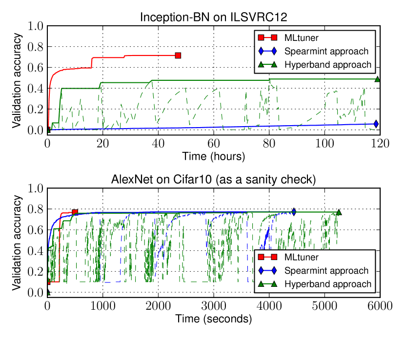
Figure 3: Runtime and accuracies of MLtuner and the state-of-the-art approaches. For Spearmint and Hyperband, the dashed curves show the accuracies of each configuration tried, and the bold curves show the maximum accuracies achieved over time.

Figure 3 shows the runtime and achieved validation accuracies of Inception-BN on ILSVRC12 and AlexNet on Cifar10. For the larger ILSVRC12 benchmark, MLtuner performs much better than Hyperband and Spearmint. After 5 days, Spearmint reached only 6% accuracy, and Hyperband reached only 49% accuracy, while MLtuner converged to 71.4% accuracy in just 2 days. The Spearmint approach performs so badly because the first tunable setting that it samples sets all tunables to their minimum values (learning rate=1e-5, momentum=0, batch size=2, data staleness=0), and the small learning rate and batch size cause the model to converge at an extremely slow rate. We have tried running Spearmint multiple times, and found their Bayesian optimization algorithm always proposes this setting as the first one to try. We also show the results on the smaller Cifar10 benchmark as a sanity check, because previous hyperparameter tuning work only reports results on this small benchmark. For the Cifar10 benchmark, all three approaches converged to approximately the same validation accuracy, but MLtuner is 9$\times$ faster than Hyperband and 3$\times$ faster than Spearmint.

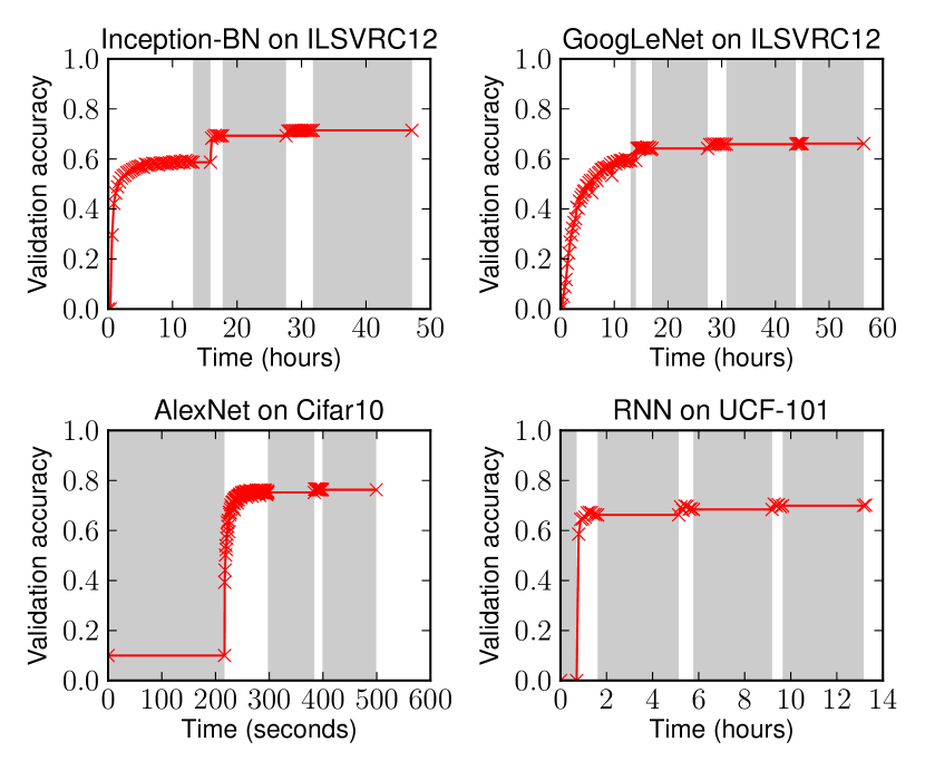
Figure 4: MLtuner tuning/re-tuning behavior on four deep learning benchmarks. The markers represent the validation accuracies measured at each epoch. The shaded time ranges are when MLtuner tunes/re-tunes tunables.

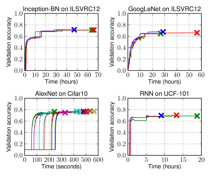
Figure 5: MLtuner results of multiple runs. The larger “x” markers mark the end of each run. The runs with the median performance are shown as the red curves in this figure and as the “MLtuner” curves in the other figures.

Compared to previous approaches, MLtuner converges to much higher accuracies in much less time. The accuracy jumps in the MLtuner curves are caused by re-tunings. Figure 4 gives a more detailed view of MLtuner’s tuning/re-tuning behavior. MLtuner re-tunes tunables when the validation accuracy plateaus, and the results shows that the accuracy usually increases after the re-tunings. This behavior echoes experts’ findings that, when training deep neural networks, it is necessary to change (usually decrease) the learning rate during training, in order to get good validation accuracies  inception-v3 ; inception-bn ; googlenet ; alexnet ; resnet ; poseidon . For the larger ILSVRC12 and RNN benchmarks, there is little overhead (2% to 6%) from the initial tuning stage, but there is considerable overhead from re-tuning, especially from the last re-tuning, when the model has already converged. That is because MLtuner assumes no knowledge of the optimal model accuracy that it is expected to achieve. Instead, it automatically finds the best achievable model accuracy via re-tuning.

Figure 5 shows the MLtuner results of multiple runs (10 runs for Cifar10 and 3 runs each for the other benchmarks). For each benchmark, MLtuner consistently converges to nearly the same validation accuracy. The number of re-tunings and convergence time are different for different runs. This variance is caused by the randomness of the HyperOpt algorithm used by MLtuner, as well as the inherent behavior of floating-point arithmetic when the values to be reduced arrive in a non-deterministic order. We observe similar behavior when not using MLtuner, due to the latter effect, which is discussed more in Section 5.4 (e.g., see Figure 9).

5.3 Tuning initial LR for adaptive LR algorithms

As we have pointed out in Section 2.3.3, the adaptive learning rate tuning algorithms, including AdaRevision adarevision , RMSProp rmsprop , Nesterov nesterov , Adam adam , AdaDelta adadelta , and AdaGrad adagrad , still require users to pick the initial learning rate. This section will show that the initial learning rate settings of those adaptive LR algorithms still greatly impact the converged model quality and convergence time, and that MLtuner can be used to tune the initial learning rate for them. For this set of experiments, MLtuner only tunes the initial learning rate, and does not re-tune, so that MLtuner will not affect the behaviors of the adaptive LR algorithms.

5.3.1 Tuning initial LR improves solution quality

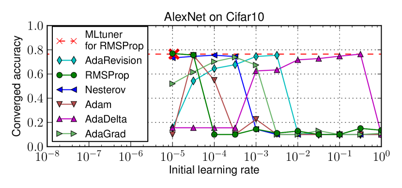
Figure 6: Converged validation accuracies when using different initial learning rates. The “x” marker marks the LR picked by MLtuner for RMSProp.

Figure 6 shows the converged validation accuracies of AlexNet on Cifar10 with different adaptive LR algorithms and different initial learning rate settings. We used the smaller Cifar10 benchmark, so that we can afford to train the model to convergence with many different initial LR settings. For the other tunables, we used the common default values (momentum=0.9, batch size=256, data staleness=0) that are frequently suggested in the literature alexnet ; googlenet ; inception-bn ; geeps . The results show that the initial LR setting greatly affects the converged accuracy, that the best initial LR settings differ across adaptive LR algorithms, and that the optimal accuracy for a given algorithm can only be achieved with one or two settings in the range. The result also shows that MLtuner can effectively pick good initial LRs for those adaptive LR algorithms, achieving close-to-ideal validation accuracy. The graph shows only the tuning result for RMSProp because of limited space, but for all the 6 adaptive LR algorithms, the accuracies achieved by MLtuner differ from those with the optimal setting by less than 2%.

5.3.2 Tuning initial LR improves convergence time

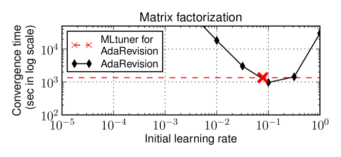
Figure 7: Convergence time when using different initial learning rates. The “x” marker marks the LR picked by MLtuner.

Figure 7 shows the convergence time when using different initial AdaRevision learning rate settings, for the matrix factorization benchmark. Because the model parameters of the MF task have uneven update frequency, practitioners often use AdaRevision adarevision to adjust its per-parameter learning rates bosen . Among all settings, more than 40% of them caused the model to converge over an order of magnitude slower than the optimal setting. We also show that, when tuning the initial LR with MLtuner, the convergence time (including the MLtuner tuning time) is close to ideal and is over an order of magnitude faster than leaving the initial LR un-tuned.

5.4 MLtuner vs. idealized manually-tuned settings

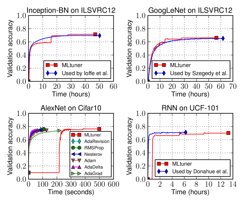
Figure 8: MLtuner compared with manually tuned settings. For comparison purpose, we have run the manually tuned settings (except for Cifar10) for long enough to ensure that their accuracies will not increase any more, rather than stopping them according to the convergence condition.

Figure 8 compares the performance of MLtuner, automatically tuning all four tunables listed in Table 3, with an idealized “manually tuned” configuration of the tunable settings. The intention is to evaluate MLtuner’s overhead relative to what an expert who already figured out the best settings (e.g., by extensive previous experimentation) might use. For the Cifar10 benchmark, we used the optimal initial LRs for the adaptive algorithms, found via running all possible settings to completion, and used effective default values for the other tunables (m=0.9, bs=256, ds=0). The results show that, among all the adaptive algorithms, RMSProp has the best performance. Compared to the best RMSProp configuration, MLtuner reaches the same accuracy, but requires about 5$\times$ more time.

For the other benchmarks, our budget does not allow us to run all the possible settings to completion to find the optimal ones. Instead, we compared with manually tuned settings suggested in the literature. For Inception-BN, we compared with the manually tuned setting suggested by Ioffe et al. in the original Inception-BN paper inception-bn , which uses an initial LR of 0.045 and decreases it by 3% every epoch. For GoogLeNet, we compared with the manually tuned setting suggested by Szegedy et al. in the original GoogLeNet paper googlenet , which uses an initial LR of 0.0015, and decreases it by 4% every 8 epochs. For RNN, we compared with the manually tuned setting suggested by Donahue et al. lrcn , which uses an initial LR of 0.001, and decreases it by 7.4% every epoch. All those manually tuned settings set momentum=0.9 and data staleness=0, and Inception-BN and GoogLeNet set batch size=32. Compared to the manually tuned settings, MLtuner achieved the same accuracies for Cifar10 and RNN, and higher accuracies for Inception-BN (71.4% vs. 69.8%) and GoogLeNet (66.2% vs. 64.4%). The higher MLtuner accuracies might be because of two reasons. First, those reported settings were tuned for potentially different hardware setups (e.g., number of machines), so they might be suboptimal for our setup. Second, those reported settings used fixed learning rate decaying rates, while MLtuner is more flexible and can use any learning rate via re-tuning.

As expected, MLtuner requires more time to train than when an expert knows the best settings to use. The difference is 5$\times$ for the small Cifar10 benchmark, but is much smaller for the larger ILSVRC12 benchmarks, because the tuning times are amortized over much more training work. We view these results to be very positive, since knowing the ML task specific settings traditionally requires extensive experimentation that significantly exceeds MLtuner’s overhead or even the much higher overheads for previous approaches like Spearmint and Hyperband.

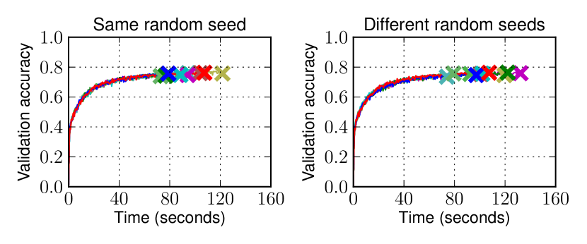
Figure 9: Performance for multiple training runs of AlexNet on Cifar10 with RMSProp and the optimal initial LR setting.

Figure 9 shows training performance for multiple runs of AlexNet with RMSProp using the same (optimal) initial LR. In the left graph, all runs initialize model parameters and shuffle training data with the same random seed. In the right graph, a distinct random seed is used for each run. We did 10 runs for each case and stopped each run when it reached the convergence condition. The result shows considerable variation in their convergence times across runs, which is caused by random initialization of parameters, training data shuffling, and non-deterministic order of floating-point arithmetic. The coefficients of variation (CoVs = standard deviation divided by average) of their convergence times are 0.16 and 0.18, respectively, and the CoVs of their converged accuracies are both 0.01. For the 10 MLtuner runs on the same benchmark shown in Figure 5, the CoV of the convergence time is 0.22, and the CoV of the converged accuracy is 0.01.

5.5 Robustness to suboptimal initial settings

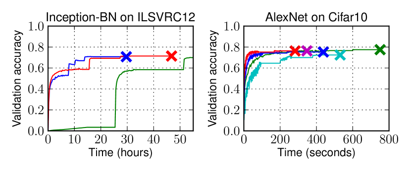
Figure 10: MLtuner performance with hard-coded initial tunable settings. The red curves used the tuned initial settings, and the other curves used randomly selected suboptimal initial settings.

This set of experiments studies the robustness of MLtuner. In particular, we turned off the initial tuning stage of MLtuner and had MLtuner use a hard-coded suboptimal tunable setting (picked randomly) as the initial setting. The result in Figure 10 shows that, even with suboptimal initial settings, MLtuner is still able to robustly converge to good validation accuracies via re-tuning.

5.6 Scalability with more tunables

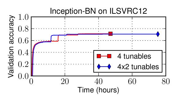
Figure 11: MLtuner performance with more tunables.

Figure 11 shows MLtuner’s scalability to the number of tunables. For the “4$\times$2 tunables” setup, we duplicated the 4 tunables listed in Table 3, making it a search space of 8 tunables. Except for making the search space larger, the added 4 tunables are transparent to the training system and do not control any other aspects of the training. The result shows that, with 8 tunables to be tuned, MLtuner still successfully converges to the same validation accuracy. The tuning time increases by about 2$\times$, which is caused by the increased number of settings tried by HyperOpt before it reaches the stopping condition.

6 Conclusions

MLtuner automatically tunes the training tunables that can have major impact on the performance and effectiveness of ML applications. Experiments with three real ML applications on two real ML systems show that MLtuner has robust performance and outperforms state-of-the-art auto-tuning approaches by over an order of magnitude on large problems. MLtuner also automatically achieves performance comparable to manually-tuned settings by experts.

References

- [1] Abadi, M., Barham, P., Chen, J., Chen, Z., Davis, A., Dean, J., Devin, M., Ghemawat, S., Irving, G., Isard, M., et al. Tensorflow: A system for large-scale machine learning. In OSDI (2016).
- [2] Ahmed, A., Aly, M., Gonzalez, J., Narayanamurthy, S., and Smola, A. J. Scalable inference in latent variable models. In WSDM (2012).
- [3] Bergstra, J., Yamins, D., and Cox, D. D. Making a science of model search: Hyperparameter optimization in hundreds of dimensions for vision architectures. ICML (1) 28 (2013).
- [4] Bergstra, J. S., Bardenet, R., Bengio, Y., and Kégl, B. Algorithms for hyper-parameter optimization. In NIPS (2011).
- [5] Bergstra, J. S., Bardenet, R., Bengio, Y., and Kégl, B. Algorithms for hyper-parameter optimization. In NIPS (2011).
- [6] Chen, T., Li, M., Li, Y., Lin, M., Wang, N., Wang, M., Xiao, T., Xu, B., Zhang, C., and Zhang, Z. MXNet: A flexible and efficient machine learning library for heterogeneous distributed systems. arXiv preprint arXiv:1512.01274 (2015).
- [7] Chilimbi, T., Suzue, Y., Apacible, J., and Kalyanaraman, K. Project Adam: Building an efficient and scalable deep learning training system. In OSDI (2014).
- [8] Cui, H., Cipar, J., Ho, Q., Kim, J. K., Lee, S., Kumar, A., Wei, J., Dai, W., Ganger, G. R., Gibbons, P. B., Gibson, G. A., and Xing, E. P. Exploiting bounded staleness to speed up big data analytics. In USENIX ATC (2014).
- [9] Cui, H., Tumanov, A., Wei, J., Xu, L., Dai, W., Haber-Kucharsky, J., Ho, Q., Ganger, G. R., Gibbons, P. B., Gibson, G. A., and Xing, E. P. Exploiting iterative-ness for parallel ML computations. In SoCC (2014).
- [10] Cui, H., Zhang, H., Ganger, G. R., Gibbons, P. B., and Xing, E. P. GeePS: Scalable deep learning on distributed GPUs with a GPU-specialized parameter server. In Proceedings of the Eleventh European Conference on Computer Systems (2016).
- [11] Dean, J., Corrado, G., Monga, R., Chen, K., Devin, M., Mao, M., Senior, A., Tucker, P., Yang, K., Le, Q. V., et al. Large scale distributed deep networks. In NIPS (2012).
- [12] Donahue, J., Hendricks, L. A., Guadarrama, S., Rohrbach, M., Venugopalan, S., Saenko, K., and Darrell, T. Long-term recurrent convolutional networks for visual recognition and description. arXiv preprint arXiv:1411.4389 (2014).
- [13] Duchi, J., Hazan, E., and Singer, Y. Adaptive subgradient methods for online learning and stochastic optimization. Journal of Machine Learning Research, Jul (2011).
- [14] Feurer, M., Klein, A., Eggensperger, K., Springenberg, J., Blum, M., and Hutter, F. Efficient and robust automated machine learning. In NIPS (2015).
- [15] Gemulla, R., Nijkamp, E., Haas, P. J., and Sismanis, Y. Large-scale matrix factorization with distributed stochastic gradient descent. In SIGKDD (2011).
- [16] He, K., Zhang, X., Ren, S., and Sun, J. Deep residual learning for image recognition. arXiv preprint arXiv:1512.03385 (2015).
- [17] Ho, Q., Cipar, J., Cui, H., Lee, S., Kim, J. K., Gibbons, P. B., Gibson, G. A., Ganger, G. R., and Xing, E. P. More effective distributed ML via a Stale Synchronous Parallel parameter server. In NIPS (2013).
- [18] Hochreiter, S., and Schmidhuber, J. Long short-term memory. Neural computation 9, 8 (1997).
- [19] Hsieh, K., Harlap, A., Vijaykumar, N., Konomis, D., Ganger, G. R., Gibbons, P. B., and Mutlu, O. Gaia: Geo-distributed machine learning approaching LAN speeds. In NSDI (2017).
- [20] Ioffe, S., and Szegedy, C. Batch normalization: Accelerating deep network training by reducing internal covariate shift. arXiv preprint arXiv:1502.03167 (2015).
- [21] Jia, Y., Shelhamer, E., Donahue, J., Karayev, S., Long, J., Girshick, R., Guadarrama, S., and Darrell, T. Caffe: Convolutional architecture for fast feature embedding. arXiv preprint arXiv:1408.5093 (2014).
- [22] Kingma, D., and Ba, J. Adam: A method for stochastic optimization. arXiv preprint arXiv:1412.6980 (2014).
- [23] Komer, B., Bergstra, J., and Eliasmith, C. Hyperopt-sklearn: automatic hyperparameter configuration for scikit-learn. In ICML workshop on AutoML (2014).
- [24] Krizhevsky, A., and Hinton, G. Learning multiple layers of features from tiny images.
- [25] Krizhevsky, A., Sutskever, I., and Hinton, G. E. ImageNet classification with deep convolutional neural networks. In NIPS (2012).
- [26] Li, L., Jamieson, K., DeSalvo, G., Rostamizadeh, A., and Talwalkar, A. Hyperband: A novel bandit-based approach to hyperparameter optimization. arXiv preprint arXiv:1603.06560 (2016).
- [27] Li, M., Andersen, D. G., Park, J. W., Smola, A. J., Ahmed, A., Josifovski, V., Long, J., Shekita, E. J., and Su, B.-Y. Scaling distributed machine learning with the parameter server. In OSDI (2014).
- [28] Maclaurin, D., Duvenaud, D., and Adams, R. P. Gradient-based hyperparameter optimization through reversible learning. In ICML (2015).
- [29] McMahan, B., and Streeter, M. Delay-tolerant algorithms for asynchronous distributed online learning. In NIPS (2014).
- [30] Močkus, J. On bayesian methods for seeking the extremum. In Optimization Techniques IFIP Technical Conference (1975), Springer.
- [31] Nesterov, Y. A method of solving a convex programming problem with convergence rate O(1/k2). In Soviet Mathematics Doklady (1983).
- [32] Ngiam, J., Coates, A., Lahiri, A., Prochnow, B., Le, Q. V., and Ng, A. Y. On optimization methods for deep learning. In Proceedings of the 28th International Conference on Machine Learning (ICML-11) (2011).
- [33] Pedregosa, F. Hyperparameter optimization with approximate gradient. arXiv preprint arXiv:1602.02355 (2016).
- [34] Power, R., and Li, J. Piccolo: Building fast, distributed programs with partitioned tables. In OSDI (2010).
- [35] Russakovsky, O., Deng, J., Su, H., Krause, J., Satheesh, S., Ma, S., Huang, Z., Karpathy, A., Khosla, A., Bernstein, M., Berg, A. C., and Fei-Fei, L. ImageNet large scale visual recognition challenge. International Journal of Computer Vision (2015).
- [36] Senior, A., Heigold, G., Yang, K., et al. An empirical study of learning rates in deep neural networks for speech recognition. In 2013 IEEE International Conference on Acoustics, Speech and Signal Processing (2013), IEEE.
- [37] Snoek, J., Larochelle, H., and Adams, R. P. Practical bayesian optimization of machine learning algorithms. In NIPS (2012).
- [38] Soomro, K., Zamir, A. R., and Shah, M. Ucf101: A dataset of 101 human actions classes from videos in the wild. arXiv preprint arXiv:1212.0402 (2012).
- [39] Sparks, E. R., Talwalkar, A., Haas, D., Franklin, M. J., Jordan, M. I., and Kraska, T. Automating model search for large scale machine learning. In SoCC (2015).
- [40] Sutskever, I., Martens, J., Dahl, G. E., and Hinton, G. E. On the importance of initialization and momentum in deep learning. ICML (2013).
- [41] Szegedy, C., Liu, W., Jia, Y., Sermanet, P., Reed, S., Anguelov, D., Erhan, D., Vanhoucke, V., and Rabinovich, A. Going deeper with convolutions. arXiv preprint arXiv:1409.4842 (2014).
- [42] Szegedy, C., Vanhoucke, V., Ioffe, S., Shlens, J., and Wojna, Z. Rethinking the inception architecture for computer vision. arXiv preprint arXiv:1512.00567 (2015).
- [43] Thornton, C., Hutter, F., Hoos, H. H., and Leyton-Brown, K. Auto-weka: Combined selection and hyperparameter optimization of classification algorithms. In SIGKDD (2013), ACM.
- [44] TielemanWang, T., and Hinton, G. Divide the gradient by a running average of its recent magnitude. COURSERA: Neural Networks for Machine Learning, 2012.
- [45] Vartak, M., Ortiz, P., Siegel, K., Subramanyam, H., Madden, S., and Zaharia, M. Supporting fast iteration in model building. NIPS ML Systems Workshop (2015).
- [46] Vinyals, O., Toshev, A., Bengio, S., and Erhan, D. Show and tell: A neural image caption generator. arXiv preprint arXiv:1411.4555 (2014).
- [47] Wei, J., Dai, W., Qiao, A., Ho, Q., Cui, H., Ganger, G. R., Gibbons, P. B., Gibson, G. A., and Xing, E. P. Managed communication and consistency for fast data-parallel iterative analytics. In SoCC (2015).
- [48] Yue-Hei Ng, J., Hausknecht, M., Vijayanarasimhan, S., Vinyals, O., Monga, R., and Toderici, G. Beyond short snippets: Deep networks for video classification. In CVPR (2015).
- [49] Zeiler, M. D. Adadelta: an adaptive learning rate method. arXiv preprint arXiv:1212.5701 (2012).
- [50] Zhang, H., Hu, Z., Wei, J., Xie, P., Kim, G., Ho, Q., and Xing, E. Poseidon: A system architecture for efficient GPU-based deep learning on multiple machines. arXiv preprint arXiv:1512.06216 (2015).