Functional renormalization-group calculation of the equation of state of one-dimensional nuclear matter inspired by the Hohenberg–Kohn theorem

Abstract

We present the first successful functional renormalization group(FRG)-aided density-functional (DFT) calculation of the equation of state (EOS) of an infinite nuclear matter (NM) in (1+1)-dimensions composed of spinless nucleons. We give a formulation to describe infinite matters in which the ’flowing’ chemical potential is introduced to control the particle number during the flow. The resultant saturation energy of the NM coincides with that obtained by the Monte-Carlo method within a few percent. Our result demonstrates that the FRG-aided DFT can be as powerful as any other methods in quantum many-body theory.

I Introduction

The Hohenberg-Kohn (HK) theorem Hohenberg and Kohn (1964) tells us that the problems of quantum many-body systems can be formulated solely in terms of the particle density $\rho(x)$ without the many-particle wave function. A formalism based on this theorem is the density functional theory (DFT) utilizing the energy density functional (EDF) $E[\rho]$. The DFT is used in various fields including quantum chemistry, condensed matter physics, and nuclear physics: Thanks to the practical methods based on the Kohn-Sham formalism Kohn and Sham (1965), DFT has become a powerful method to analyze the properties of ground states; see Refs. Kohn (1999); Kryachko and Ludeña (2014); Zangwill (2015); Jones (2015) for an overview. Methods to investigate excited states such as the time-dependent density functional theory Runge and Gross (1984) have also been developed Ullrich (2012); Nakatsukasa et al. (2016).

It should be, however, noted that the HK theorem only guarantees the existence of the EDF $E[\rho]$ which could be minimized to obtain the exact ground-state density and energy, but does not provide any theoretical prescription to construct $E[\rho]$ itself. Thus most practical calculations utilize $E[\rho]$ that is constructed in a semi-empirical way. Hence developing a systematic method to derive $E[\rho]$ from microscopic Hamiltonian still remains as a fundamental problem in the field of quantum many-body theory.

A clue of this fundamental problem may be provided by the notion of effective field theory developed in quantum field theory. Indeed the two-particle point-irreducible (2PPI) effective action Verschelde and Coppens (1992) can lead to an energy density functional written in terms of $\rho$ for which the HK theorem naturally emerges Polonyi and Sailer (2002); Schwenk and Polonyi (2004). A nice point with the effective-action approach is that an established powerful computational machinery is now available, which is called the functional renormalization group (FRG) method Wetterich (1993); Wegner and Houghton (1973); Wilson and Kogut (1974); Polchinski (1984). In this method, the quantum fluctuations are gradually taken into account from an ultraviolet to infrared scale by solving the one-parameter flow equation of the scale-dependent effective action, and hence a coarse-grained effective action is eventually obtained; see Refs. Berges et al. (2002); Gies (2012); Pawlowski (2007) for reviews. Since the 2PPI effective action is a generalization of the energy density functional, the FRG method formulated for the 2PPI action possibly gives a formal foundation to DFT and provides a long-desired method for constructing the density functional from a microscopic Hamiltonian, as initiated by Polonyi, Sailer and Schwenk Polonyi and Sailer (2002); Schwenk and Polonyi (2004). Such an observation has lead to a notion of DFT-RG or 2PPI-FRG method Braun (2012); Kemler and Braun (2013); Kemler et al. (2017); Kemler (2017); Liang et al. (2018), which is a quite attractive scheme for solving the fundamental problem in the field of the DFT: In a pioneering work Kemler and Braun (2013), accurate ground state energies of simple toy models in quantum mechanics are obtained within the fourth-order truncation: A recent paper Liang et al. (2018) proposed an efficient method to incorporate the higher-order correlations, and the method was applied to a $0$-dimensional quartic model successfully. The subsequent analysis of a one-dimensional system composed of a finite number of particles motivated by the nuclear saturation problem Kemler et al. (2017); Kemler (2017), however, showed that the second-order truncation only gives a 30% accuracy in comparison with the result of the Monte-Carlo simulation Alexandrou et al. (1989). Possible improvement of the result may be obtained by an incorporation of the higher-order correlation functions as suggested in the demonstration in a 0-dimensional model Liang et al. (2018).

In this paper, we apply the DFT-RG scheme to an infinite uniform system. Our point is that an infinite system with a definite particle density may be well described with first few correlation functions while rarefied systems are interaction-dominating systems and higher correlation functions may play significant roles. Needless to say, an infinite uniform system is a fundamentally important system for understanding many-body physics and indeed the local density approximation for $E[\rho]$ was found to be unexpectedly successful Kohn and Sham (1965). We give a DFT-RG formalism for infinite matters in which we introduce a ’flowing’ chemical potential to control the flow of the particle number caused by switching on the inter-particle interaction. Then we calculate the equation of state (EOS) of an infinite nuclear matter (NM) in (1+1)-dimensions composed of spinless nucleons as in Refs. Alexandrou et al. (1989); Kemler et al. (2017). Starting from the two-’nucleon’ interaction constructed in Ref. Alexandrou et al. (1989) where the saturation curve of the one-dimensional NM is obtained by the Monte-Carlo simulation, we solve the flow equation for the 2PPI effective action with some reasonable truncation. We show that the resultant density functional $E[\rho]$ nicely gives the saturation energy, i.e. the minimum of the energy derived by the EOS with respect to the density, that coincides with that of the Monte Carlo method Alexandrou et al. (1989).

This paper is organized as follows: In Sec. II, our formalism is shown. We introduce the flowing chemical potential to control the particle number during the flow and derive the DFT-RG flow equation for infinite uniform systems with a definite particle number. In Sec. III, we apply our formalism to a (1+1)-dimensional spinless nuclear matter. The results of the density dependence of the ground state energy, i.e. the equation of state is shown in this section. Section IV is devoted to the conclusion.

II Formalism

In this section, we show our formalism to analyze ground state energies of one-dimensional continuum matters composed of spinless fermions in the framework of DFT-RG.

We consider (1+1)-dimensional spinless fermions with a two-body interaction $U$. We employ the imaginary-time finite-temperature formalism for convenience. Then the action in the units such that mass of a fermion is $1$ reads

$$S[\psi^{*},\psi] =\int_{\chi}\psi^{*}(\chi_{\epsilon})\left(\partial_{\tau}-\frac{\partial^{2}_{x}}{2}\right)\psi(\chi)$$

$$+\frac{1}{2}\int_{\chi,\chi^{\prime}}U_{\rm 2b}(\chi,\chi^{\prime})\psi^{*}(\chi_{\epsilon})\psi^{*}(\chi^{\prime}_{\epsilon})\psi(\chi^{\prime})\psi(\chi),$$ (1)

where $\chi:=(\tau,x)$, $\chi_{\epsilon}:=(\tau+\epsilon,x)$ with a positive infinitesimal $\epsilon$, $\int_{\chi}:=\int_{\tau}\int_{x}:=\int_{0}^{\beta}d\tau\int dx$ with an inverse temperature $\beta$, and $U_{\rm 2b}(\chi,\chi^{\prime}):=U_{\rm 2b}(\chi-\chi^{\prime}):=\delta(\tau-\tau^{\prime})U(x-x^{\prime})$. The imaginary times of the fermion fields $\psi$ and $\psi^{*}$ at the same point are infinitesimally different, which comes from the construction of the path integral formalism Altland and Simons (2010).

Following the prescription in Ref. Polonyi and Sailer (2002); Schwenk and Polonyi (2004), we introduce the regulated interaction $U_{\rm 2b,\lambda}(\chi)$ ($U_{\lambda}$(x)) such that $U_{\rm 2b,\lambda=0}(\chi)=0$ and $U_{\rm 2b,\lambda=1}(\chi)=U_{\rm 2b}(\chi)$ ($U_{\lambda=0}(x)=0$ and $U_{\lambda=1}(x)=U(x)$). Then the regulated action is defined in terms of $U_{\rm 2b,\lambda}(\chi)$:

$$S_{\lambda}[\psi^{*},\psi] =\int_{\chi}\psi^{*}(\chi)\left(\partial_{\tau}-\frac{\partial^{2}_{x}}{2}\right)\psi(\chi)$$

$$+\frac{1}{2}\int_{\chi,\chi^{\prime}}U_{\rm 2b,\lambda}(\chi,\chi^{\prime})\psi^{*}(\chi_{\epsilon})\psi^{*}(\chi^{\prime}_{\epsilon})\psi(\chi^{\prime})\psi(\chi).$$ (2)

This action becomes that for free particles at $\lambda=0$ and Eq. (1) at $\lambda=1$. The parameter $\lambda\in[0,1]$ is interpreted as the flow parameter from the free to interacting system. In this paper, we choose $U_{\rm 2b,\lambda}(\chi,\chi^{\prime})=\lambda U_{\rm 2b}(\chi,\chi^{\prime})$.

The EDF $E_{\lambda}[\rho]$ realizing the HK theorem can be defined in terms of the 2PPI effective action Fukuda et al. (1994), which is defined as follows:

$$\Gamma_{\lambda}[\rho]=\sup_{J}\left(\int_{\chi}J(\chi)\rho(\chi)-W_{\lambda}[J]\right),$$ (3)

where $\rho(\chi)$ is the density field, $W_{\lambda}[J]:=\ln Z_{\lambda}[J]$ is the generating functional for the connected density correlation functions and $Z_{\lambda}[J]=\int\mathcal{D}\psi^{*}\mathcal{D}\psi\exp(-S_{\lambda}[\psi^{*},\psi]+\int_{\chi}J(\chi)\rho_{\psi}(\chi))$ is the generating functional for the correlation functions of the density field $\rho_{\psi}(\chi)=\psi^{*}(\chi_{\epsilon})\psi(\chi)$. To see the correspondence of the 2PPI effective action to the EDF, we consider the variational problem of $\Gamma_{\lambda}[\rho]$ with a fixed number of particles. The stationary condition of the effective action determines the behavior of the expectation value of the density field. Under the constraint that the number of particles is fixed, we should minimize $I_{\lambda}[\rho]:=\Gamma_{\lambda}[\rho]-\mu_{\lambda}\int_{\chi}\rho(\chi)$ with respect to $\rho(\chi)$. In general, the Fermi energy, and the particle number, depend on the interaction and change during the flow. We thus have introduced a $\lambda$-dependent Lagrange multiplier, or physically a ’flowing’ chemical potential, $\mu_{\lambda}$ to control the particle number during the flow. The ground state density $\rho_{\rm gs,\lambda}(\chi)$ satisfies the stationary condition:

$$\Gamma^{(1)}_{\lambda}[\rho_{\rm gs,\lambda}](\chi)=J_{\rm sup}[\rho_{\rm gs,\lambda}](\chi)=\mu_{\lambda},$$ (4)

where $J_{\rm sup}[\rho](\chi)$ is $J(\chi)$ maximizing the right hand side of Eq. (3) and

$$\Gamma_{\lambda}^{(n)}[\rho](\chi_{1},\cdots,\chi_{n}):=\frac{\delta^{n}\Gamma[\rho]}{\delta\rho(\chi_{1})\cdots\delta\rho(\chi_{n})}.$$

Because $-W_{\lambda}[\mu_{\lambda}]/\beta$ is the grand potential, we have $\Gamma_{\lambda}[\rho_{\rm gs,\lambda}]=\mu_{\lambda}\int_{\chi}\rho_{\rm gs,\lambda}(\chi)-W_{\lambda}[\mu_{\lambda}]=\beta F_{\lambda}$, where $F_{\lambda}$ is the Helmholtz free energy. At the zero temperature limit $\beta\to\infty$, $\Gamma_{\lambda}[\rho_{\rm gs,\lambda}]/\beta$ becomes the ground state energy $E_{\rm gs,\lambda}$ because $F_{\lambda}$ can be written as $F_{\lambda}=-\beta^{-1}\ln\sum_{n}\exp(-\beta E_{n,\lambda})$, where $\{E_{n,\lambda}\}$ is the energy eigenvalues of the system and satisfies $E_{\rm gs,\lambda}=E_{0,\lambda}<E_{1,\lambda}<\cdots$. Therefore $\Gamma_{\lambda}[\rho]$ can be related to the EDF:

$$E_{\lambda}[\rho]=\lim_{\beta\to\infty}\frac{\Gamma_{\lambda}[\rho]}{\beta}.$$ (5)

$\rho_{\rm gs,\lambda}(\chi)$ is uniquely determined because of the convexity of the effective action except for the case when the eigenvalues of $\Gamma^{(2)}_{\lambda}[\rho_{\rm gs,\lambda}](\chi,\chi^{\prime})$ do not satisfy positivity, which implies that the ground state is unstable Polonyi and Sailer (2002).

The flow equation of $\Gamma_{\lambda}[\rho]$ is derived by differentiating Eq. (3) with respect to $\lambda$: $\partial_{\lambda}\Gamma_{\lambda}[\rho]=-(\partial_{\lambda}W_{\lambda})[J_{\rm sup,\lambda}[\rho]].$ The right-hand side of this flow equation becomes

$$- (\partial_{\lambda}W_{\lambda})[J_{\rm sup,\lambda}[\rho]]$$

$$= \frac{1}{2}\int_{\chi,\chi^{\prime}}\dot{U}_{\rm 2b,\lambda}(\chi,\chi^{\prime})\braket{\psi^{*}(\chi_{\epsilon})\psi^{*}(\chi^{\prime}_{\epsilon})\psi(\chi^{\prime})\psi(\chi)}_{\rho}$$

$$= \frac{1}{2}\int_{\chi,\chi^{\prime}}\dot{U}_{\rm 2b,\lambda}(\chi,\chi^{\prime})\left(\braket{\rho_{\psi}(\chi)}_{\rho}\braket{\rho_{\psi}(\chi^{\prime})}_{\rho}\right.$$

$$+\left.W_{\lambda}^{(2)}[J_{\rm sup,\lambda}[\rho]](\chi,\chi^{\prime})-\delta(x-x^{\prime})\braket{\rho_{\psi}(\chi)}_{\rho}\right),$$ (6)

where $\dot{U}_{\rm 2b,\lambda}(\chi,\chi^{\prime}):=\partial_{\lambda}U_{\rm 2b,\lambda}(\chi,\chi^{\prime})$,

$$\braket{\cdots}_{\rho}:= \int\mathcal{D}\psi^{*}\mathcal{D}\psi\cdots\frac{{\rm e}^{-S_{\lambda}[\psi^{*},\psi]+\int_{\chi}J_{\rm sup,\lambda}[\rho](\chi)\rho_{\psi}(\chi)}}{Z_{\lambda}[J_{\rm sup,\lambda}[\rho]]},$$

and

$$W_{\lambda}^{(n)}[J](\chi_{1},\cdots,\chi_{n}):=\frac{\delta^{n}W_{\lambda}[J]}{\delta J(\chi_{1})\cdots\delta J(\chi_{n})}.$$

To derive Eq. (6), we have used $U_{\rm 2b}(\chi,\chi^{\prime})\sim\delta(\tau-\tau^{\prime})$ and the canonical commutation relation: $\langle\psi^{*}(\tau+\epsilon,x)(\psi^{*}(\tau+\epsilon,x^{\prime})\psi(\tau,x^{\prime})+\psi(\tau+\epsilon,x^{\prime})\psi^{*}(\tau,x^{\prime}))\psi(\tau,x)\rangle_{\rho}=\delta(x-x^{\prime})\langle\rho_{\psi}(\chi)\rangle_{\rho}$. We note that $\braket{\cdots}_{\rho}$ gives averages for imaginary-time-ordered operator products and that the density–density correlation function $W_{\lambda}^{(2)}[J_{\rm sup,\lambda}[\rho]](\chi,\chi^{\prime})$ at $\tau=\tau^{\prime}$ should be interpreted as $\lim_{\tau\to\tau^{\prime}}\lim_{\epsilon\to+0}(\braket{\psi^{*}(\chi_{\epsilon})\psi(\chi)\psi^{*}(\chi^{\prime}_{\epsilon})\psi(\chi^{\prime})}_{\rho}-\braket{\psi^{*}(\chi_{\epsilon})\psi(\chi)}_{\rho}\braket{\psi^{*}(\chi^{\prime}_{\epsilon})\psi(\chi^{\prime})}_{\rho})$ where the limit $\tau\to\tau^{\prime}$ is taken after the limit $\epsilon\to+0$, i.e. $|\tau^{\prime}-\tau|>\epsilon$. By use of the relations $\braket{\rho_{\psi}(\chi)}_{\rho}=W^{(1)}_{\lambda}[J_{\rm sup,\lambda}](\chi)=\rho(\chi)$ and

$$\int_{\chi^{\prime}}\Gamma^{(2)}_{\lambda}[\rho](\chi,\chi^{\prime})W^{(2)}_{\lambda}[J_{\rm sup,\lambda}[\rho]](\chi^{\prime},\chi^{\prime\prime})$$

$$=\int_{\chi^{\prime}}\frac{\delta J_{\rm sup,\lambda}[\rho](\chi)}{\delta\rho(\chi^{\prime})}\frac{\delta\rho(\chi^{\prime})}{\delta J_{\rm sup,\lambda}[\rho](\chi^{\prime\prime})}=\delta(\chi,\chi^{\prime\prime})$$

the flow equation can be written in term of $\Gamma_{\lambda}[\rho]$ Schwenk and Polonyi (2004); Kemler et al. (2017):

$$\partial_{\lambda}\Gamma_{\lambda}[\rho]= \frac{1}{2}\int_{\chi,\chi^{\prime}}\dot{U}_{\rm 2b,\lambda}(\chi,\chi^{\prime})\left(\rho(\chi)\rho(\chi^{\prime})\right.$$

$$+\left.\Gamma_{\lambda}^{(2)-1}[\rho](\chi,\chi^{\prime})-\rho(\chi)\delta(x-x^{\prime})\right).$$ (7)

where $\Gamma_{\lambda}^{(2)-1}[\rho](\chi,\chi^{\prime})$ is the inverse of $\Gamma_{\lambda}^{(2)}[\rho](\chi,\chi^{\prime})$.

In principle, the functional flow equation (7) with the effective action $\Gamma_{0}[\rho]$ for the free fermions gives the effective action $\Gamma_{1}[\rho]$ for the interacting fermions. In general, however, some approximation is needed for the practical use of Eq. (7). Here, we employ the vertex expansion:

$$\Gamma_{\lambda}[\rho]= \Gamma_{\lambda}[\rho_{\rm gs,\lambda}]+\sum_{n=1}^{\infty}\int_{\chi_{1}}\cdots\int_{\chi_{n}}\Gamma_{\lambda}^{(n)}[\rho_{\rm gs,\lambda}](\chi_{1},\cdots,\chi_{n})$$

$$\times(\rho(\chi_{1})-\rho_{\rm gs,\lambda}(\chi_{1}))\cdots(\rho(\chi_{n})-\rho_{\rm gs,\lambda}(\chi_{n})).$$

Up to the second order expansion, Eq. (7) is rewritten as the following flow equations:

$$\partial_{\lambda}\Gamma_{\lambda}[\rho_{\rm gs,\lambda}]= \int_{\chi}\Gamma_{\lambda}^{(1)}[\rho_{\rm gs,\lambda}](\chi)\partial_{\lambda}\rho_{\rm gs,\lambda}+\frac{1}{2}\int_{\chi,\chi^{\prime}}\dot{U}_{\rm 2b,\lambda}(\chi,\chi^{\prime})\left(\rho_{\rm gs,\lambda}(\chi)\rho_{\rm gs,\lambda}(\chi^{\prime})\right.$$

$$+\left.\Gamma_{\lambda}^{(2)-1}[\rho_{\rm gs,\lambda}](\chi,\chi^{\prime})-\rho_{\rm gs,\lambda}(\chi)\delta(x-x^{\prime})\right),$$ (8)

$$\partial_{\lambda}\Gamma_{\lambda}^{(1)}[\rho_{\rm gs,\lambda}](\chi)= \int_{\chi^{\prime}}\Gamma^{(2)}_{\lambda}[\rho_{\rm gs,\lambda}](\chi,\chi^{\prime})\partial_{\lambda}\rho_{\rm gs,\lambda}(\chi^{\prime})+\int_{\chi^{\prime}}\dot{U}_{\rm 2b,\lambda}(\chi,\chi^{\prime})\rho_{\rm gs,\lambda}(\chi^{\prime})-\frac{1}{2}\dot{U}_{\lambda}(0)$$

$$-\frac{1}{2}\int_{\chi_{1},\chi_{2},\chi_{3},\chi_{4}}\dot{U}_{\rm 2b,\lambda}(\chi_{4},\chi_{1})\Gamma_{\lambda}^{(2)-1}[\rho_{\rm gs,\lambda}](\chi_{1},\chi_{2})\Gamma_{\lambda}^{(3)}[\rho_{\rm gs,\lambda}](\chi_{2},\chi_{3},\chi)\Gamma_{\lambda}^{(2)-1}[\rho_{\rm gs,\lambda}](\chi_{3},\chi_{4}),$$ (9)

$$\partial_{\lambda}\Gamma_{\lambda}^{(2)}[\rho_{\rm gs,\lambda}](\chi,\chi^{\prime})= \int_{\chi_{1}}\Gamma^{(3)}_{\lambda}[\rho_{\rm gs,\lambda}](\chi,\chi^{\prime},\chi_{1})\partial_{\lambda}\rho_{\rm gs,\lambda}(\chi_{1})+\dot{U}_{\rm 2b,\lambda}(\chi,\chi^{\prime})$$

$$-\frac{1}{2}\int_{\chi_{1},\cdots,\chi_{4}}\dot{U}_{\rm 2b,\lambda}(\chi_{4},\chi_{1})\Gamma_{\lambda}^{(2)-1}[\rho_{\rm gs,\lambda}](\chi_{1},\chi_{2})\Gamma_{\lambda}^{(4)}[\rho_{\rm gs,\lambda}](\chi_{2},\chi_{3},\chi,\chi^{\prime})\Gamma_{\lambda}^{(2)-1}[\rho_{\rm gs,\lambda}](\chi_{3},\chi_{4})$$

$$+\int_{\chi_{1},\cdots,\chi_{6}}\dot{U}_{\rm 2b,\lambda}(\chi_{4},\chi_{1})\Gamma_{\lambda}^{(2)-1}[\rho_{\rm gs,\lambda}](\chi_{1},\chi_{2})\Gamma_{\lambda}^{(3)}[\rho_{\rm gs,\lambda}](\chi_{2},\chi_{3},\chi)$$

$$\times\Gamma_{\lambda}^{(2)-1}[\rho_{\rm gs,\lambda}](\chi_{3},\chi_{4})\Gamma_{\lambda}^{(3)}[\rho_{\rm gs,\lambda}](\chi_{4},\chi_{5},\chi^{\prime})\Gamma_{\lambda}^{(2)-1}[\rho_{\rm gs,\lambda}](\chi_{5},\chi_{6}).$$ (10)

These flow equation can be simplified by rewriting in terms of the connected correlation functions:

$$G^{(n)}_{\lambda}(\chi_{1},\cdots,\chi_{n})=W_{\lambda}^{(n)}[J_{\rm sup}[\rho_{\rm gs,\lambda}]](\chi_{1},\cdots,\chi_{n}).$$

$\Gamma^{(n)}_{\lambda}[\rho_{\rm gs,\lambda}]$ is related to the connected correlation functions with the following relation:

$$\Gamma_{\lambda}^{(n)}[\rho_{\rm gs,\lambda}](\chi_{1},\cdots,\chi_{n})=\left.\left(\prod_{i=1}^{n-2}\int_{\chi^{\prime}_{i}}W_{\lambda}^{(2)-1}[J](\chi_{i},\chi^{\prime}_{i})\frac{\delta}{\delta J(\chi^{\prime}_{i})}\right)W_{\lambda}^{(2)-1}[J](\chi_{n-1},\chi_{n})\right|_{J=J_{\rm sup}[\rho_{\rm gs,\lambda}]},$$

which is derived from the following identity:

$$\frac{\delta}{\delta\rho(\chi)}=\int_{\chi^{\prime}}\frac{\delta J_{\rm sup,\lambda}[\rho](\chi^{\prime})}{\delta\rho(\chi)}\frac{\delta}{\delta J_{\rm sup,\lambda}(\chi^{\prime})}=\int_{\chi^{\prime}}W_{\lambda}^{(2)-1}[J_{\sup,\lambda}[\rho]](\chi,\chi^{\prime})\frac{\delta}{\delta J_{\rm sup,\lambda}(\chi^{\prime})}.$$ (11)

The relations between $\Gamma_{\lambda}^{(2,3,4)}[\rho_{\rm gs,\lambda}]$ and the connected correlation functions read

$$\Gamma_{\lambda}^{(2)}[\rho_{\rm gs,\lambda}](\chi_{1},\chi_{2})= G^{(2)-1}_{\lambda}(\chi_{1},\chi_{2})$$

$$\Gamma_{\lambda}^{(3)}[\rho_{\rm gs,\lambda}](\chi_{1},\chi_{2},\chi_{3})= -\int_{\chi^{\prime}_{1},\chi^{\prime}_{2},\chi^{\prime}_{3}}G^{(3)}_{\lambda}(\chi^{\prime}_{1},\chi^{\prime}_{2},\chi^{\prime}_{3})G^{(2)-1}_{\lambda}(\chi_{1},\chi^{\prime}_{1})G^{(2)-1}_{\lambda}(\chi_{2},\chi^{\prime}_{2})G^{(2)-1}_{\lambda}(\chi_{3},\chi^{\prime}_{3})$$

$$\Gamma_{\lambda}^{(4)}[\rho_{\rm gs,\lambda}](\chi_{1},\chi_{2},\chi_{3}.\chi_{4})= -\int_{\chi^{\prime}_{1},\chi^{\prime}_{2},\chi^{\prime}_{3}.\chi^{\prime}_{4}}G^{(4)}_{\lambda}(\chi^{\prime}_{1},\chi^{\prime}_{2},\chi^{\prime}_{3},\chi^{\prime}_{4})G^{(2)-1}_{\lambda}(\chi_{1}\chi^{\prime}_{1})G^{(2)-1}_{\lambda}(\chi_{2},\chi^{\prime}_{2})G^{(2)-1}_{\lambda}(\chi_{3},\chi^{\prime}_{3})G^{(2)-1}_{\lambda}(\chi_{4},\chi^{\prime}_{4})$$

$$+\int_{\chi^{\prime}_{1},\chi^{\prime}_{2},\chi^{\prime}_{3}}G^{(2)-1}_{\lambda}(\chi_{2},\chi^{\prime}_{2})G^{(2)-1}_{\lambda}(\chi_{3},\chi^{\prime}_{3})G^{(3)}_{\lambda}(\chi^{\prime}_{1},\chi^{\prime}_{2},\chi^{\prime}_{3})$$

$$\times G^{(2)-1}_{\lambda}(\chi^{\prime}_{5},\chi^{\prime}_{1})G^{(3)}_{\lambda}(\chi^{\prime}_{4},\chi^{\prime}_{5},\chi^{\prime}_{6})G^{(2)-1}_{\lambda}(\chi_{1},\chi^{\prime}_{4})G^{(2)-1}_{\lambda}(\chi_{4},\chi^{\prime}_{6})$$

$$+\int_{\chi^{\prime}_{1},\chi^{\prime}_{2},\chi^{\prime}_{3}}G^{(2)-1}_{\lambda}(\chi_{4},\chi^{\prime}_{2})G^{(2)-1}_{\lambda}(\chi_{3},\chi^{\prime}_{3})G^{(3)}_{\lambda}(\chi^{\prime}_{1},\chi^{\prime}_{2},\chi^{\prime}_{3})$$

$$\times G^{(2)-1}_{\lambda}(\chi^{\prime}_{5},\chi^{\prime}_{1})G^{(3)}_{\lambda}(\chi^{\prime}_{4},\chi^{\prime}_{5},\chi^{\prime}_{6})G^{(2)-1}_{\lambda}(\chi_{1},\chi^{\prime}_{4})G^{(2)-1}_{\lambda}(\chi_{2},\chi^{\prime}_{6})$$

$$+\int_{\chi^{\prime}_{1},\chi^{\prime}_{2},\chi^{\prime}_{3}}G^{(2)-1}_{\lambda}(\chi_{2},\chi^{\prime}_{2})G^{(2)-1}_{\lambda}(\chi_{4},\chi^{\prime}_{3})G^{(3)}_{\lambda}(\chi^{\prime}_{1},\chi^{\prime}_{2},\chi^{\prime}_{3})$$

$$\times G^{(2)-1}_{\lambda}(\chi^{\prime}_{5},\chi^{\prime}_{1})G^{(3)}_{\lambda}(\chi^{\prime}_{4},\chi^{\prime}_{5},\chi^{\prime}_{6})G^{(2)-1}_{\lambda}(\chi_{1},\chi^{\prime}_{4})G^{(2)-1}_{\lambda}(\chi_{3},\chi^{\prime}_{6}).$$

By use of these relations, Eqs. (8)-(10) are rewritten as follows:

$$\partial_{\lambda}\Gamma_{\lambda}[\rho_{\rm gs,\lambda}]= \int_{\chi}\mu_{\lambda}\partial_{\lambda}\rho_{\rm gs,\lambda}(\chi)+\frac{1}{2}\int_{\chi,\chi^{\prime}}\dot{U}_{\rm 2b,\lambda}(\chi,\chi^{\prime})\left(\rho_{\rm gs,\lambda}(\chi)\rho_{\rm gs,\lambda}(\chi^{\prime})+G_{\lambda}^{(2)}(\chi,\chi^{\prime})-\rho_{\rm gs,\lambda}(\chi^{\prime})\delta(x^{\prime}-x)\right),$$ (12)

$$\partial_{\lambda}\rho_{\rm gs,\lambda}(\chi)= -\frac{1}{2}\int_{\chi_{1},\chi_{2}}\dot{U}_{\rm 2b,\lambda}(\chi_{1},\chi_{2})G_{\lambda}^{(3)}(\chi_{2},\chi_{1},\chi)$$

$$+\int_{\chi_{1}}G_{\lambda}^{(2)}(\chi,\chi_{1})\left(\partial_{\lambda}\mu_{\lambda}-\int_{\chi_{2}}\dot{U}_{\rm 2b,\lambda}(\chi_{1},\chi_{2})\rho_{\rm gs,\lambda}(\chi_{2})+\frac{1}{2}\dot{U}_{\lambda}(0)\right),$$ (13)

$$\partial_{\lambda}G_{\lambda}^{(2)}(\chi,\chi^{\prime})= -\int_{\chi_{1},\chi_{2}}\dot{U}_{\rm 2b,\lambda}(\chi_{1},\chi_{2})\left(G_{\lambda}^{(2)}(\chi,\chi_{1})G_{\lambda}^{(2)}(\chi_{2},\chi^{\prime})+\frac{1}{2}G_{\lambda}^{(4)}(\chi_{2},\chi_{1},\chi,\chi^{\prime})\right)$$

$$+\int_{\chi_{1}}G_{\lambda}^{(3)}(\chi,\chi^{\prime},\chi_{1})\left(\partial_{\lambda}\mu_{\lambda}-\int_{\chi_{2}}\dot{U}_{\rm 2b,\lambda}(\chi_{1},\chi_{2})\rho_{\rm gs,\lambda}(\chi_{2})+\frac{1}{2}\dot{U}_{\lambda}(0)\right).$$ (14)

Here, we have used Eqs. (4) and (5). These flow equations determine the behavior of the free energy $\Gamma_{\lambda}[\rho_{\rm gs,\lambda}]=\beta F_{\lambda}$, the ground state density $\rho_{\rm gs,\lambda}(\chi)$ and the density–density correlation function $G_{\lambda}^{(2)}(\chi,\chi^{\prime})$ under a given $\lambda$-dependent chemical potential $\mu_{\lambda}$.

For the case of free fermion $\lambda=0$, the ground state of the system is homogeneous. In this paper, we assume that the homogeneity of the system remains even if $\lambda\neq 0$, i.e. the transition to an inhomogeneous state does not occur even if the interaction is switched on. In general, the switching on of the interaction at $\lambda\neq 0$ changes the density as represented in Eq. (13). However, we can compensate this effect of the interaction by choosing an appropriate $\mu_{\lambda}$ and realize $\partial_{\lambda}\rho_{\rm gs,\lambda}=0$ in the case of the homogeneous system. We employ the momentum representation for convenience to discuss how to choose $\mu_{\lambda}$. In the momentum representation, Eqs. (12)-(14) in the case of homogeneous states read

$$\partial_{\lambda}\frac{\Gamma_{\lambda}[\rho_{\rm gs,\lambda}]}{\beta V}= \mu_{\lambda}\partial_{\lambda}\rho_{\rm gs,\lambda}+\frac{1}{2}\tilde{U}(0)\rho_{\rm gs,\lambda}^{2}+\frac{1}{2}\int_{p}\tilde{U}(p)\left(T\sum_{\omega}\tilde{G}^{(2)}_{\lambda}(P)-\rho_{\rm gs,\lambda}\right),$$ (15)

$$\partial_{\lambda}\rho_{\rm gs,\lambda}= -\frac{1}{2}\int_{P}\tilde{U}(p)\tilde{G}_{\lambda}^{(3)}(P,-P)+\tilde{G}_{\lambda}^{(2)}(0)\left(\partial_{\lambda}\mu_{\lambda}-\tilde{U}(0)\rho_{\rm gs,\lambda}+\frac{1}{2}U(0)\right),$$ (16)

$$\partial_{\lambda}\tilde{G}_{\lambda}^{(2)}(P)= -\tilde{U}(p)G_{\lambda}^{(2)}(P)^{2}-\frac{1}{2}\int_{P^{\prime}}\tilde{U}(p^{\prime})\tilde{G}^{(4)}_{\lambda}(P^{\prime},-P^{\prime},P)+G_{\lambda}^{(3)}(P,-P)\left(\partial_{\lambda}\mu_{\lambda}-\tilde{U}(0)\rho_{\rm gs,\lambda}+\frac{1}{2}U(0)\right).$$ (17)

Here we have used $U_{\rm 2b,\lambda}(\chi,\chi^{\prime})=\lambda U(x-x^{\prime})\delta(\tau-\tau^{\prime})$ and introduced the volume of the system $V$ and the Fourier transformations $\tilde{U}(p):=\int_{x}U(x)e^{-ipx}$ and $(2\pi)^{2}\delta(P_{1}+\cdots+P_{n})\tilde{G}_{\lambda}^{(n)}(P_{1},\cdots,P_{n-1}):=\int_{\chi_{1},\cdots,\chi_{n}}e^{-i(P_{1}\cdot\chi_{1}+\cdots+P_{n}\cdot\chi_{n})}G_{\lambda}^{(n)}(\chi_{1},\cdots,\chi_{n})$, where $P_{i}:=(\omega_{i},p_{i})$ is a vector of a Matsubara frequency and a momentum. We have introduced the short hands $\int_{p}:=\int dp/(2\pi)$ and $\int_{P}:=\int_{p}T\sum_{\omega}$. Then $\partial_{\lambda}\rho_{\rm gs,\lambda}=0$ is realized if the flow of $\mu_{\lambda}$ is set as follows:

$$\partial_{\lambda}\mu_{\lambda}= \tilde{U}(0)\rho_{\rm gs,\lambda}-\frac{U(0)}{2}+\int_{P}\frac{\tilde{U}(p)\tilde{G}_{\lambda}^{(3)}(P,-P)}{2\tilde{G}_{\lambda}^{(2)}(0)}.$$ (18)

We note that $\tilde{G}_{\lambda}^{(2)}(0)$ should be interpreted as the $p$ limit of $\tilde{G}_{\lambda}^{(2)}(P)$: $\tilde{G}_{\lambda}^{(2)}(0)=\lim_{p\to 0}\tilde{G}^{(2)}_{\lambda}(0,p)$, because the Matsubara frequency $\omega$ is discrete. The $p$ limit of the $\tilde{G}^{(2)}_{\lambda}(P)$ is the static particle-density susceptibility and generally nonzero, while $\lim_{p\to 0}\tilde{G}^{(2)}_{\lambda}(P)=0$ with a finite frequency Forster (1975); Kunihiro (1991); Fujii and Ohtani (2004). This is in contrast to the case of a finite number of particles in a finite box Kemler et al. (2017), where density correlation functions with vanishing frequency and momentum were interpreted as the $\omega$ limit, i.e., not only $\int dx_{i}G_{\lambda}^{(n)}(\chi_{1},\cdots,\chi_{n})=0$ but also $\int_{\chi_{i}}G_{\lambda}^{(n)}(\chi_{1},\cdots,\chi_{n})=0$ with $i\in\{1,\cdots,n\}$ were used to derive the flow equations.

In this paper, we focus on the zero temperature limit. In the zero temperature limit with the condition Eq. (18), Eqs. (15) and (17) becomes as follows:

$$\partial_{\lambda}\overline{E}_{\rm gs,\lambda}= \frac{\rho_{\rm gs,0}}{2}\tilde{U}(0)+\frac{1}{2\rho_{\rm gs,0}}\int_{p}\tilde{U}(p)\left(\int_{\omega}\tilde{G}^{(2)}_{\lambda}(P)-\rho_{\rm gs,0}\right),$$ (19)

$$\partial_{\lambda}\tilde{G}_{\lambda}^{(2)}(P)= -\tilde{U}(p)\tilde{G}_{\lambda}^{(2)}(P)^{2}-\frac{1}{2}\int_{P^{\prime}}\tilde{U}(p^{\prime})\tilde{G}^{(4)}_{\lambda}(P^{\prime},-P^{\prime},P)+\int_{P^{\prime}}\frac{\tilde{U}(p^{\prime})\tilde{G}_{\lambda}^{(3)}(P^{\prime},-P^{\prime})\tilde{G}_{\lambda}^{(3)}(P,-P)}{2\tilde{G}_{\lambda}^{(2)}(0)},$$ (20)

where we have introduced the energy per particle $\overline{E}_{\rm gs,\lambda}=\lim_{\beta\to 0}\Gamma_{\lambda}[\rho_{\rm gs,\lambda}]/(\beta\int_{x}\rho_{\rm gs,0})$ and the shorthand $\int_{\omega}=\int d\omega/(2\pi)$.

The flow equation for $G^{(n)}_{\lambda}$ generally depends on $G^{(m\leq n+2)}_{\lambda}$, which means that an infinite series of coupled flow equations emerges. We avoid to treat such an infinite series of coupled flow equations by ignoring the flows of $G_{\lambda}^{(3\leq n)}$. However, we do not simply substitute $\tilde{G}_{\lambda}^{(3,4)}$ for $\tilde{G}_{0}^{(3,4)}$ in Eq. (20). Such a simple replacement breaks a constraint for multi-particle distribution functions imposed by the Pauli blocking: By use of the canonical commutation relation, the $n$-particle distribution function $f_{n,\lambda}(x_{1},\cdots,x_{n})=\lim_{\epsilon\rightarrow+0}\braket{\psi^{*}(\epsilon,x_{1})\cdots\psi^{*}(\epsilon,x_{n})\psi(0,x_{n})\cdots\psi(0,x_{1})}_{\rho_{\rm gs,\lambda}}$ is related to the connected correlation functions $G_{\lambda}^{(m\leq n)}$. Because of the Pauli blocking, the distribution function satisfies $f_{n,\lambda}(x_{1},\cdots,x_{n})=0$ if $x_{i}=x_{j}$ for $i\neq j$. In the case of $n=2$, the relation between $f_{2,\lambda}(x_{1},x_{2})$ and $G_{\lambda}^{(2)}$ is derived in the same same manner as the aforementioned derivation of Eq. (6):

$$f_{2,\lambda}(x_{1},x_{2})$$

$$= \braket{\rho_{\psi}(0,x_{1})\rho_{\psi}(0,x_{2})}_{\rho_{\rm gs,\lambda}}-\delta(x_{1}-x_{2})\braket{\rho_{\psi}(0,x_{1})}_{\rho_{\rm gs,\lambda}}$$

$$= G_{\lambda}^{(2)}(0,x_{1},0,x_{2})+\rho_{\rm gs,\lambda}(x_{1})\rho_{\rm gs,\lambda}(x_{2})$$

$$-\delta(x_{1}-x_{2})\rho_{\rm gs,\lambda}(x_{1}).$$

Then the condition imposed by the Pauli blocking reads

$$\lim_{x_{1}\rightarrow x_{2}}G_{\lambda}^{(2)}(0,x_{1},0,x_{2})$$

$$= \lim_{x_{1}\rightarrow x_{2}}\left(\delta(x_{1}-x_{2})\rho_{\rm gs,\lambda}(x_{1})-\rho_{\rm gs,\lambda}(x_{1})\rho_{\rm gs,\lambda}(x_{2})\right).$$

In our case, the right-hand side of this condition does not depend on $\lambda$: $\lim_{x_{1}\rightarrow x_{2}}\partial_{\lambda}G_{\lambda}^{(2)}(0,x_{1},0,x_{2})=0$, because $\partial_{\lambda}\rho_{\rm gs,\lambda}=0$. Therefore, from Eq. (20), the following condition should be satisfied:

$$-\int_{P}\tilde{U}(p)\tilde{G}_{\lambda}^{(2)}(P)^{2}-\frac{1}{2}\int_{P,P^{\prime}}\tilde{U}(p^{\prime})\tilde{G}^{(4)}_{\lambda}(P^{\prime},-P^{\prime},P)$$

$$+\int_{P,P^{\prime}}\frac{\tilde{U}(p^{\prime})\tilde{G}_{\lambda}^{(3)}(P^{\prime},-P^{\prime})\tilde{G}_{\lambda}^{(3)}(P,-P)}{2\tilde{G}_{\lambda}^{(2)}(0)}=0$$ (21)

This condition, however, is broken by the simple substitution $\tilde{G}_{\lambda}^{(3,4)}$ for $\tilde{G}_{0}^{(3,4)}$. To respect the condition Eq. (21), we approximate the second and third terms in the right-hand side of Eq. (20) as follows Kemler et al. (2017):

$$-\frac{1}{2}\int_{P^{\prime}}\tilde{U}(p^{\prime})\tilde{G}^{(4)}_{\lambda}(P^{\prime},-P^{\prime},P)$$

$$+\int_{P^{\prime}}\frac{\tilde{U}(p^{\prime})\tilde{G}_{\lambda}^{(3)}(P^{\prime},-P^{\prime})\tilde{G}_{\lambda}^{(3)}(P,-P)}{2\tilde{G}_{\lambda}^{(2)}(0)}$$

$$\approx c_{\lambda}\left(-\frac{1}{2}\int_{P^{\prime}}\tilde{U}(p^{\prime})\tilde{G}^{(4)}_{0}(P^{\prime},-P^{\prime},P)\right.$$

$$+\left.\int_{P^{\prime}}\frac{\tilde{U}(p^{\prime})\tilde{G}_{0}^{(3)}(P^{\prime},-P^{\prime})\tilde{G}_{0}^{(3)}(P,-P)}{2\tilde{G}_{0}^{(2)}(0)}\right)$$ (22)

where $c_{\lambda}$ is the factor to preserve the condition Eq. (21):

$$c_{\lambda} =\int_{P}\tilde{U}(p)\tilde{G}_{\lambda}^{(2)}(P)^{2}$$

$$\times\left(-\frac{1}{2}\int_{P^{\prime},P^{\prime\prime}}\tilde{U}(p^{\prime})\tilde{G}^{(4)}_{0}(P^{\prime},-P^{\prime},P^{\prime\prime})\right.$$

$$+\left.\int_{P^{\prime},P^{\prime\prime}}\frac{\tilde{U}(p^{\prime})\tilde{G}_{0}^{(3)}(P^{\prime},-P^{\prime})\tilde{G}_{0}^{(3)}(P^{\prime\prime},-P^{\prime\prime})}{2\tilde{G}_{0}^{(2)}(0)}\right)^{-1}.$$

At $\lambda=0$, we have $c_{0}=1$. In our approximation, the contribution of diagrams such as multi-pair creations is not included. Such diagrams are important to investigate the spectral properties of one-dimensional fermion systems Pustilnik et al. (2006); Teber (2007); Imambekov et al. (2012), which is beyond the scope of this paper.

$$\tilde{G}_{0}^{(2)}(P) =\parbox[c]{75.0001pt}{ \includegraphics[width=75.0001pt]{G2_0}}$$

$$\tilde{G}_{0}^{(3)}(P_{1},P_{2}) =\parbox[c]{70.0001pt}{ \includegraphics[width=70.0001pt]{G3_0_1}}+\parbox[c]{70.0001pt}{ \includegraphics[width=70.0001pt]{G3_0_2}}$$

$$\tilde{G}_{0}^{(4)}(P_{1},P_{2},P_{3}) =\parbox[c]{70.0001pt}{ \includegraphics[width=70.0001pt]{G4_0_1}}+\parbox[c]{70.0001pt}{ \includegraphics[width=70.0001pt]{G4_0_2}}$$

$$+\parbox[c]{70.0001pt}{ \includegraphics[width=70.0001pt]{G4_0_4}}+\parbox[c]{70.0001pt}{ \includegraphics[width=70.0001pt]{G4_0_6}}$$

$$+\parbox[c]{70.0001pt}{ \includegraphics[width=70.0001pt]{G4_0_3}}+\parbox[c]{70.0001pt}{ \includegraphics[width=70.0001pt]{G4_0_5}}$$

Figure 1: The diagrammatic representations of $\tilde{G}_{0}^{(2,3,4)}$. The solid line is the free fermion propagator $\tilde{G}_{\rm F,0}^{(2)}(P)$. In the diagrams for $\tilde{G}_{0}^{(3)}$ and $\tilde{G}_{0}^{(4)}$, $P_{3}=-P_{1}-P_{2}$ and $P_{4}=-P_{1}-P_{2}-P_{3}$, respectively.

We specify the initial conditions $\overline{E}_{\rm gs,\lambda=0}$, $\rho_{\rm gs,\lambda=0}$, and $\tilde{G}^{(2,3,4)}_{\lambda=0}$. We denote $\rho_{\rm gs,0}$ as $n$, which is the ground state density during the flow, and in particular at $\lambda=1$, because $\rho_{\rm gs,\lambda}(\chi)=\rho_{\rm gs,0}$. The fermi momentum and fermi energy are defined as $p_{\rm F}=\pi n$ and $E_{\rm F}=p_{\rm F}^{2}/2$, respectively. $\overline{E}_{\rm gs,\lambda=0}$ is the ground state energy per particle of a one-dimensional free Fermi gas: $\overline{E}_{\rm gs,0}=E_{\rm F}/3$. $\tilde{G}^{(2,3,4)}_{\lambda=0}$ are the density correlation functions for free fermions:

$$\tilde{G}^{(2)}_{0}(P)= -\int_{P^{\prime}}\tilde{G}_{\rm F,0}^{(2)}(P^{\prime})\tilde{G}_{\rm F,0}^{(2)}(P+P^{\prime}),$$

$$\tilde{G}^{(3)}_{0}(P_{1},P_{2})= -\sum_{\sigma\in S_{2}}\int_{P^{\prime}}\tilde{G}_{\rm F,0}^{(2)}(P^{\prime})\tilde{G}_{\rm F,0}^{(2)}(P_{\sigma(1)}+P^{\prime})$$

$$\times\tilde{G}_{\rm F,0}^{(2)}(P_{\sigma(1)}+P_{\sigma(2)}+P^{\prime}),$$

$$\tilde{G}^{(4)}_{0}(P_{1},P_{2},P_{3})= -\sum_{\sigma\in S_{3}}\int_{P^{\prime}}\tilde{G}_{\rm F,0}^{(2)}(P^{\prime})\tilde{G}_{\rm F,0}^{(2)}(P_{\sigma(1)}+P^{\prime})$$

$$\times\tilde{G}_{\rm F,0}^{(2)}(P_{\sigma(1)}+P_{\sigma(2)}+P^{\prime})$$

$$\times\tilde{G}_{\rm F,0}^{(2)}(P_{\sigma(1)}+P_{\sigma(2)}+P_{\sigma(3)}+P^{\prime}).$$

Here $S_{2}$ and $S_{3}$ are the symmetric groups of order two and three, respectively, and $\tilde{G}_{\rm F,0}^{(2)}(P)$ is the two-point propagator of free fermions: $\tilde{G}_{\rm F,0}^{(2)}(P)={1}/(i\omega-\xi(p))$, where $\xi(p):=p^{2}/2-E_{\rm F}$. The diagrammatic representations of these correlation functions are shown in Fig. 1. The explicit forms of $\tilde{G}^{(2)}_{0}(P)$ and the second and third terms of the right-hand side of Eq. (20) after the frequency integral under the approximation Eq. (22) becomes as follows:

$$\tilde{G}^{(2)}_{0}(P)=\int_{p^{\prime}}\frac{2\theta(\xi(p+p^{\prime}))\theta(-\xi(p^{\prime}))\left(\xi(p+p^{\prime})-\xi(p^{\prime})\right)}{\omega^{2}+[\xi(p+p^{\prime})-\xi(p^{\prime})]^{2}},$$ (23)

$$-\frac{c_{\lambda}}{2}\int_{P^{\prime}}\tilde{U}(p^{\prime})\tilde{G}^{(4)}_{0}(P^{\prime},-P^{\prime},P)+c_{\lambda}\int_{P^{\prime}}\frac{\tilde{U}(p^{\prime})\tilde{G}_{0}^{(3)}(P^{\prime},-P^{\prime})\tilde{G}_{0}^{(3)}(P,-P)}{2\tilde{G}_{0}^{(2)}(0)}$$

$$=2c_{\lambda}\int_{p^{\prime},p^{\prime\prime}}\tilde{U}(p^{\prime})\theta(-\xi(p^{\prime}+p^{\prime\prime}))(\theta(-\xi(p^{\prime\prime}+p))-\theta(-\xi(p^{\prime\prime})))\left[\frac{(\xi(p^{\prime\prime}+p)-\xi(p^{\prime\prime}))^{2}-\omega^{2}}{(\omega^{2}+(\xi(p^{\prime\prime}+p)-\xi(p^{\prime\prime}))^{2})^{2}}\right.$$

$$\quad+\left.\frac{2\theta(\xi(p^{\prime\prime}+p+p^{\prime}))}{\xi(p^{\prime\prime}+p^{\prime}+p)-\xi(p^{\prime\prime}+p)-\xi(p^{\prime\prime}+p^{\prime})+\xi(p^{\prime\prime})}\frac{\xi(p^{\prime\prime}+p+p^{\prime})-\xi(p^{\prime\prime}+p^{\prime})}{\omega^{2}+(\xi(p^{\prime\prime}+p+p^{\prime})-\xi(p^{\prime\prime}+p^{\prime}))^{2}}\right].$$ (24)

The flow equations (19) and (20) under the approximation Eq. (22) with the expression Eq. (24) are found to be the same as those obtained from the continuum limit of the system with finite number of particles in a finite box presented in Kemler et al. (2017). Finally we comment on the derivation of Eq. (24). Both terms in the left-hand side of Eq. (24) have delta functions in the momentum integrals, which comes from the derivatives of the distribution functions of fermions such as $\theta^{\prime}(-\xi(p^{\prime}))=-\delta(\xi(p^{\prime}))$. These contributions from the delta functions, however, cancel each other out and do not appear in the final expression in Eq. (24).

III Demonstration in one-dimensional spinless nuclear matter

In this section, we demonstrate the calculation of the ground state energy as a function of the density, i.e. the equation of state (EOS) in a $(1+1)$-dimensional spinless continuum nuclear matter Alexandrou et al. (1989).

III.1 One-dimensional spinless nuclear matter

We consider a $(1+1)$-dimensional continuum matter composed of spinless fermions with the following two-body interaction Alexandrou et al. (1989):

$$U(r)=\frac{g}{\sqrt{\pi}}\left(\frac{1}{\sigma_{1}}{\rm e}^{-\frac{r^{2}}{\sigma_{1}^{2}}}-\frac{1}{\sigma_{2}}{\rm e}^{-\frac{r^{2}}{\sigma_{2}^{2}}}\right)$$

where $\sigma_{1}>0$, $\sigma_{2}>0$ and $g>0$. In this model, the short-range repulsive force and long-range attractive force between nucleons are represented with the superposition of the two Gaussians. Following Ref. Alexandrou et al. (1989), we choose $g=12$, $\sigma_{1}=0.2$ and $\sigma_{2}=0.8$ in units such that the mass of a nucleon is 1. These parameters are determined under the assumption that some dimensionless quantities obtained in the $(3+1)$-dimensional system empirically are reproduced also in $(1+1)$ dimension.

In this model, the ground state energy of the continuum nuclear matter is derived from the extrapolation of the ground state energies of the systems with 2 to 12 nucleons calculated by the Monte Carlo (MC) simulation at a given density which seems to be close to the saturation density Alexandrou et al. (1989). Although there may be some discrepancy between the energy derived from the MC simulation and the saturation energy due to the choice of the density, we use the energy derived from the MC simulation as a reference of the saturation energy to benchmark our result.

III.2 Numerical procedure

We mention some details of our numerical analysis to solve the flow equations.

Equations (24) has a seemingly singular point at $p^{\prime}=0$ in the term proportional to $(\xi(p^{\prime\prime}+p^{\prime}+p)-\xi(p^{\prime\prime}+p)-\xi(p^{\prime\prime}+p^{\prime})+\xi(p^{\prime\prime}))^{-1}\sim p^{\prime-1}$ in the integrand. This singularity, however, vanishes because $\tilde{U}(p^{\prime}=0)=0$ for our interaction. To avoid the division-by-zero operation, we rewrite the integrand as a manifestly regular form for the numerical calculation by use of the Maclaurin expansion of $\tilde{U}(p^{\prime})$.

In order to calculate $\tilde{G}^{(2)}_{\lambda}(\omega,p)$ on the $(\omega,p)$-plane, we discretize $\omega$ and $p$. We change $\omega$ to $\bar{\omega}=(2/\pi)\arctan(\omega/s)$, where $s$ is an arbitral number, and discretize $\bar{\omega}$ in the domain $[-1,1]$. We set a cutoff $\Lambda=\max(10p_{\rm F},1)$ for momentum $p$. We have checked that the result hardly depends on $\Lambda$ even if it is set to larger values.

III.3 Ground state properties

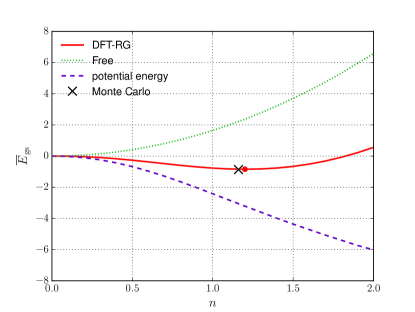
Figure 2: Energy per particle $\overline{E}_{\rm gs}$ as a function of density $n$ in the case of DFT-RG (solid red line). The energy of free fermion (green dotted line), the contribution from the inter-nucleon potential (purple dashed line) and the result of the extrapolated energy given by a MC simulation Alexandrou et al. (1989) at a density close but not equal to saturation density (black cross) are also shown. The red point is the saturation point derived from the DFT-RG calculation. The units for $\overline{E}_{\rm gs}$ and $n$ are such that the mass of a nucleon is $1$.

Table 1: The saturation energies $\overline{E}_{\rm s}$ derived from the first-order perturbation, DFT-RG with $c_{\lambda}=1$, DFT-RG, and the MC simulation Alexandrou et al. (1989). Their relative errors compared to the result of the Monte Carlo simulation $\overline{E}_{\rm s,MC}$ and the saturation densities $\rho_{\rm s}$ are also shown. The units for $\overline{E}_{\rm s}$ and $\rho_{\rm s}$ are such that the mass of a nucleon is $1$.

	1st order	DFT-RG ($c_{\lambda}=1$)	DFT-RG	Monte Carlo Alexandrou et al. (1989)
$\left|\overline{E}_{\rm s}\right|$	0.780	0.827	0.844	0.867
$\left|\left(\overline{E}_{\rm s}-\overline{E}_{\rm s,MC}\right)/\overline{E}_{\rm s,MC}\right|$ (%)	10.0	4.6	2.7	-
$\rho_{\rm s}$	1.19	1.21	1.20	-

We show our result of the EOS together with the energy of the free Fermi gas $\overline{E}_{\rm gs,0}$ and the contribution from the inter-nucleon potential $\overline{E}_{\rm gs,1}-\overline{E}_{\rm gs,0}$ in Fig. 2. The free case shows an increase with respect to $n$, which reflects that the average kinetic energy increases because the fermi sphere becomes larger as $n$ increases. On the other hand, the contribution from the inter-particle potential reduces the energy because it has a long-range attractive part. The competition between these contributions results in the emergence of a minimum point at a finite $n$, i.e. the saturation point.

To discuss the quantitative aspects of our result, we show our result of the EOS near the saturation point in Fig. 3.

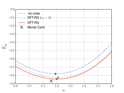
Figure 3: Energy per particle $\overline{E}_{\rm gs}$ as a function of density $n$ near the saturation point. The result of DFT-RG (solid red line), first-order perturbation (blue dashed line), DFT-RG with $c_{\lambda}=1$ (green dotted–dashed line), and a MC simulation Alexandrou et al. (1989) (black cross) are shown. The density $n=1.16$ used in the MC simulation is an assumed one which is close but not equal to saturation density. The units for $\overline{E}_{\rm gs}$ and $n$ are such that the mass of a nucleon is $1$.

For comparison, the results with the first-order perturbation and with ignoring the running of $c_{\lambda}$, i.e. $c_{\lambda}=1$, are also shown. In our formalism, the first-order perturbation is reproduced when $\tilde{G}^{(2)}_{\lambda}(P)$ in Eq. (19) is replaced with $\tilde{G}^{(2)}_{0}(P)$. In Fig. 3, one finds that the saturation energy derived from DFT-RG is closer to the result of the MC simulation than any other methods. We again note that the density used in the MC result shown in Fig. 3 is not a calculated but given density which is assumed to be close but not equal to the saturation density. Therefore, the density used in the MC simulation should not be used as a reference of the benchmark of the saturation density.

Table 1 shows the numerical results of the saturation energy $\overline{E}_{\rm s}$ and density $\rho_{\rm s}$ derived from each method. As shown in this table, the deviation of the saturation energy between DFT-RG and the MC simulation is only 2.7%. Compared to the result of the first-order perturbation, the accuracy of $\overline{E}_{\rm s}$ is largely improved by use of the DFT-RG scheme. Moreover, the introduction of the running of the factor $c_{\lambda}$ also contributes to the improvement of the accuracy. Although there is no reference for the saturation density $\rho_{\rm s}$, it seems to converge to a value near $1.20$.

IV Conclusion

In this paper, we have presented the functional renormalization group (FRG)-aided density-functional theory (DFT) calculation of the equation of state of an infinite nuclear matter in (1+1)-dimensions composed of spinless nucleons. We have shown a novel formalism to treat infinite matters in which the flow of the chemical potential is taken into account to control the particle number during the flow. The resultant saturation energy coincides with that obtained from the Monte-Carlo simulation within a few percent. Thus one sees that DFT-RG scheme works well for the infinite homogeneous nuclear system around the saturation point in comparison with the case of finite nuclear system Kemler et al. (2017) where the same approximation for the flow equations was employed: A truncation including up to the second-order vertex expansion was used and an approximation was made for the three- and four-point correlation functions so that the Pauli blocking effect is taken into account.

Our result together with its numerical feasibility clearly demonstrate that the DFT-RG scheme is a promising nonperturbative method to analyze quantum many-body systems, at least, composed of infinite number of particles. One of the next steps is applying our method to higher-dimensional systems which should be easy in the present grand canonical formalism. The extension to a finite-temperature case can be done as well. The extension to particles with internal degrees of freedom Kemler (2017) is also an important future direction.

Another interesting extension of the present work is calculation of dynamical quantities. One of the basic quantities for analyzing the dynamical properties is the spectral functions. Recently, the FRG has been developed so that the spectral functions can be calculated which describe the dynamical properties of the system Kamikado et al. (2014); Tripolt et al. (2014a, b); Yokota et al. (2016, 2017). It is intriguing to extend the DFT-RG scheme so that the spectral function can be calculated. We have already calculated the spectral function of the density–density correlation function in the DFT-RG scheme for the one-dimensional model used in this work. We will report the analysis of the spectral function in a separate paper, where some relevance to the Tomonaga-Luttinger liquid with a non-linear dispersion relation Imambekov et al. (2012) will be discussed. In conclusion, the present work demonstrates that the FRG-aided DFT scheme can be as powerful as any other methods in quantum many-body theory.