K2-231 b: A sub-Neptune exoplanet transiting a solar twin in Ruprecht 147

Abstract

We identify a sub-Neptune exoplanet ($R_{p}=2.5\pm 0.2$ $\mbox{R}_{\earth}$) transiting a solar twin in the Ruprecht 147 star cluster (3 Gyr, 300 pc, [Fe/H] = +0.1 dex). The $\sim$81 day light-curve for EPIC 219800881 ($V=12.71$) from K2 Campaign 7 shows six transits with a period of 13.84 days, a depth of $\sim$0.06%, and a Based on our analysis of high-resolution MIKE spectra, broadband optical and NIR photometry, the cluster parallax and interstellar reddening, and isochrone models from PARSEC, Dartmouth, and MIST, we estimate the following properties for the host star: $M_{\star}=$ 1.01 $\pm$ 0.03 $\mbox{M}_{\odot}$, $R_{\star}=$ 0.95 $\pm$ 0.03 $\mbox{R}_{\odot}$, and $T_{\mbox{\scriptsize eff}}=$ 5695 $\pm$ 50 K. This star appears to be single based on our modeling of the photometry, the low radial velocity (RV) variability measured over nearly ten years, and Keck/NIRC2 adaptive optics imaging and aperture-masking interferometry. Applying a probabilistic mass–radius relation, we estimate that the mass of this planet is $M_{p}=7+5-3$ $\mbox{M}_{\earth}$, which would cause an RV semi-amplitude of $K=2\pm 1$ $\mbox{m s}^{-1}$ that may be measurable with existing precise RV facilities. After statistically validating this planet with BLENDER, we now designate it K2-231 b, making it the second substellar object to be discovered in Ruprecht 147 and the first planet; it joins the small but growing ranks of 22 other planets and 3 candidates found in open clusters.

1 Introduction

Transit and Doppler surveys have detected thousands of exoplanets, and modeling their rate of occurrence shows that approximately one in three Sun-like stars hosts at least one planet with an orbital period under 29 days (Fressin et al., 2013). Stars tend to form in clusters from the gravitational collapse and fragmentation of molecular clouds (Lada & Lada, 2003), so it is natural to expect that stars still existing in clusters likewise host planets at a similar frequency. In fact, circumstellar disks have been observed in very young clusters and moving groups (2.5–30 Myr; Haisch et al., 2001). However, some have speculated that stars forming in denser cluster environments (i.e., the kind that can remain gravitationally bound for billions of years) will be exposed to harsher conditions than stars formed in looser associations or that join the Galactic field relatively quickly after formation, and this will impact the frequency of planets formed and presently existing in star clusters. For example, stars in a rich and dense cluster might experience multiple supernovae during the planet-forming period (the lifetime of a 10 $\mbox{M}_{\odot}$ star is $\sim$30 Myr), as well as intense FUV radiation from their massive star progenitors that can photoevaporate disks. Furthermore, stars in denser clusters ($\sim$0.3–30 FGK stars pc^-3) will also dynamically interact with other stars (and binary/multiple systems) at a higher frequency than more isolated stars in the field ($\sim$0.06 stars pc^-3), which might tend to disrupt disks and/or eject planets from their host star systems.

These concerns have been addressed theoretically and with observations (Scally & Clarke, 2001; Smith & Bonnell, 2001; Bonnell et al., 2001; Adams et al., 2006; Fregeau et al., 2006; Malmberg et al., 2007; Spurzem et al., 2009; de Juan Ovelar et al., 2012; Vincke & Pfalzner, 2016; Kraus et al., 2016; Cai et al., 2017), and all of these factors were considered by Adams (2010) in evaluating the birth environment of the solar system, but progress in this field necessitates that we actually detect and characterize planets in star clusters and determine their frequency of occurrence.

1.1 Planets Discovered in Open Clusters

Soon after the discovery of the first known exoplanet orbiting a Sun-like star (Mayor & Queloz, 1995), Janes (1996) suggested open clusters as ideal targets for photometric monitoring. Two decades later, we still only know of a relatively small number of exoplanets existing in open clusters. One observational challenge has been that the majority of nearby star clusters are young, and therefore their stars are rapidly rotating and magnetically active. Older clusters with inactive stars tend to be more distant, and their Sun-like stars are likewise too faint for most Doppler and ground-based transit facilities. The first planets discovered in open clusters with the Doppler technique were either massive Jupiters or potentially brown dwarfs: Lovis & Mayor (2007) found two substellar objects in NGC 2423 and NGC 4349; Sato et al. (2007) detected a companion to a giant star in the Hyades; Quinn et al. (2012) discovered two hot Jupiters in Praesepe (known as the “two b’s in the Beehive,” one of which also has a Jupiter-mass planet in a long-period, eccentric orbit; Malavolta et al., 2016), and Quinn et al. (2014) discovered another in the Hyades; and, finally, nontransiting hot Jupiters have been found in M67 around three main-sequence stars, one Jupiter was detected around an evolved giant, and three other planet candidates were identified (Brucalassi et al., 2014, 2016, 2017).

NASA’s Kepler mission changed this by providing high-precision photometry for four clusters (Meibom et al., 2011). Two sub-Neptune-sized planets were discovered in the 1 Gyr NGC 6811 cluster, and Meibom et al. (2013) concluded that planets occur in that dense environment ($N=377$ stars) at roughly the same frequency as in the field. After Kepler was repurposed as K2, many more clusters were observed for $\sim$80 days each, and as a result, many new cluster planets have been identified. Many of these are hosted by lower-mass stars that are intrinsically faint and difficult to reach with existing precision radial velocity (RV) facilities from Earth. So far, results have been reported from K2 monitoring of the following clusters, listed in order of increasing age: Gaidos et al. (2017) reported zero detections in the Pleiades (see also Mann et al., 2017). Mann et al. (2016a) and David et al. (2016a) independently discovered a Neptune-sized planet transiting a M4.5 dwarf in the Hyades; recently Mann et al. (2018) reported three Earth-to-Neptune-sized planets orbiting a mid-K dwarf in the Hyades (K2-136), while Ciardi et al. (2018) concurrently announced the Neptune-sized planet and that this K dwarf formed a binary with a late-M dwarf; the system was later reported on by Livingston et al. (2018). In Praesepe, Obermeier et al. (2016) announced K2-95 b, a Neptune-sized planet orbiting an M dwarf, which was later studied by Libralato et al. (2016), Mann et al. (2017), and Pepper et al. (2017); adding the planets found by Pope et al. (2016), Barros et al. (2016), Libralato et al. (2016), and Mann et al. (2017), there are six confirmed planets (including K2-100 through K2-104) and one candidate that were validated by Mann et al. (2017). Finally, Nardiello et al. (2016) reported three planetary candidates in the M67 field, although all appear to be nonmembers.

Table A lists the 23 planets and 3 candidates that have been discovered in clusters so far, including K2-231 b. Of these, 15 transit their host stars, and all but six of the hosts are fainter than $V>13$, which makes precise RV follow-up prohibitively expensive. These hosts are all relatively young ($\sim$650 Myr) and magnetically active and thus might still present a challenge to existing Doppler facilities and techniques. Such RV observations are required to measure masses and determine the densities of these planets.

1.2 The K2 Survey of Ruprecht 147

Ruprecht 147 was also observed by K2 during Campaign 7. Curtis et al. (2013) demonstrated that R147 is the oldest nearby star cluster, with an age of 3 Gyr at a distance of 300 pc (see also the Ph.D. dissertation of Curtis, 2016). According to Howell et al. (2014), planets only a few times larger in size than Earth would be detectable around dwarfs at least as bright as $K_{p}<16$, which approximately corresponds to an M0 dwarf with $M=0.6$ $\mbox{M}_{\odot}$ in R147 . Soon after the public release of the Campaign 7 light-curves, we discovered a substellar object transiting a solar twin in Ruprecht 147 (EPIC 219388192; CWW 89A from Curtis et al. 2013), which we determined was a warm brown dwarf in an eccentric $\sim$5 day orbit, and we announced our discovery at the 19th Cambridge Workshop on Cool Stars, Stellar Systems, and the Sun (“Cool Stars 19”) in Uppsala, Sweden (Curtis et al., 2016). Nowak et al. (2017) independently discovered and characterized this system.

Now we report the identification of an object transiting a different solar twin in R147 (CWW 93 from Curtis et al., 2013), which we show is a sub-Neptune exoplanet. We made this discovery while reviewing and comparing light-curves from various groups for our stellar rotation program , and noticed a repeating shallow transit pattern spaced at $\sim$14 days in the EVEREST light-curve for EPIC 219800881 (Luger et al., 2016, 2017).

In this paper, we describe our production of a light-curve, which we model to derive the properties of the exoplanet (Section 2). We also characterize the host star and check for stellar binary companionship (Section 3), and test false-positive scenarios in order to statistically validate the exoplanet (Section 4).

K2-231 was also targeted by the following programs: “Statistics of Variability in Main-Sequence Stars of Kepler 2 Fields 6 and 7” (PI: Guzik; GO 7016), “The Masses and Prevalence of Small Planets with K2 – Cycle 2” (PI: Howard; GO 7030), and “K2 follow-up of the nearby, old open cluster Ruprecht 147” (PI: Nascimbeni; GO 7056).

2 K2 Light-curve Analysis

The top panel of Figure 1 shows the EVEREST light-curve for EPIC 219800881 that caught our attention. We then downloaded the calibrated pixel-level data from the Barbara A. Mikulski Archive for Space Telescopes (MAST), extracted a light-curve, and corrected for K2 systematic effects following Vanderburg & Johnson (2014). We confirmed the transits detected by eye with a Box-fitting Least-Squares (BLS) periodogram search (Kovács et al., 2002). The BLS periodogram identified a strong signal at a 13.844 day period with a transit depth of approximately 0.06%. We then refined the light-curve by simultaneously fitting the K2 pointing systematics, a low-frequency stellar activity signal (modeled with a basis spline with breakpoints spaced every 0.75 days), and transits (using Mandel & Agol 2002 models), as described in Section 4 of Vanderburg et al. (2016). Deviating from our standard procedure of using stationary apertures, we opted to use a smaller, moving circular aperture with a radius of $9^{\prime\prime}$ (2.32 pixels) in order to exclude many nearby background stars (see Figure 3 and Table 4). The middle panel of Figure 1 shows the detrended version of our extracted light-curve using the best-fit low-frequency model produced during the light-curve calibration.

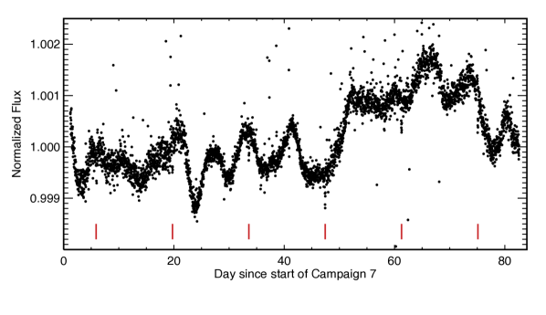
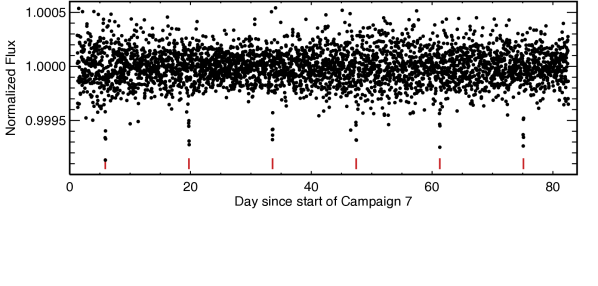
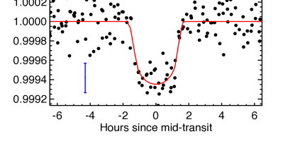
Figure 1: K2 light-curves for EPIC 219800881: (Top) The EVEREST light-curve used to visually identify the transiting object, with the transits marked as short red vertical lines at the bottom of the figure. (Middle) Our refined and detrended light-curve, extracted with a $9^{\prime\prime}$ circular moving aperture while simultaneously fitting the pointing systematics, activity signal, and transits following Vanderburg et al. (2016), with the transits similarly marked. (Bottom) Our detrended light-curve, phase-folded according to the 13.842 day period, along with the model for highest-likelihood solution from the ZEIT transit-fit procedure (see Table 1), sampled at the times of observation according to the 30 minute integration cadence (red).

The determination of the physical radius of the planet candidate and size of its orbit requires an accurate characterization of the host star, which we present in Section 3. In this work, we adopt the following conventions from IAU 2015 Resolution B3 for the nominal radii for the Sun and Earth, which we apply to convert the measured transit quantities $a/R_{\star}$ and $R_{p}/R_{\star}$ to physical and terrestrial units (Mamajek et al., 2015; Prša et al., 2016): $1~{}\hbox{$(\mathcal{R})^{\rm N}_{\odot}$}=6.957\times 10^{8}$ m and $1~{}\hbox{$(\mathcal{R})_{\earth}^{\rm N}$}=6.3781\times 10^{6}$ m, where this nominal terrestrial radius is Earth’s “zero tide” equatorial value.

We modeled the light-curve with EXOFAST (Eastman et al., 2013). EXOFAST is an IDL-based transit and RV fitter for solving single-planet systems that employs the Mandel & Agol (2002) analytic light-curve model, limb darkening parameters from Claret & Bloemen (2011), and accounts for the long 30 minute K2 cadence. EXOFAST requires prior information on the time of transit and the period of the orbit; the stellar temperature, metallicity, and surface gravity; and, without radial velocities (RVs), Eastman et al. recommended fixing the orbit geometry to circular, as the light-curve does not provide adequate constraints on eccentricity or the argument of periastron.

Next, we modeled the light-curve following the procedure applied in the Zodiacal Exoplanets In Time (ZEIT) program, described in Mann et al. (2016a, 2017, 2018), which employs model light-curves generated with the BAsic Transit Model cAlculatioN code (batman; Kreidberg, 2015) and the quadratic limb-darkening law sampling method from Kipping (2013). We also accounted for the 30 minute cadence and assigned a Gaussian prior on the stellar density of $\rho_{\star}=1.17\pm 0.12~{}\rho_{\odot}$ derived from our estimates of the star’s mass and radius. The posterior distributions of the various model parameters were sampled with the affine-invariant Markov chain Monte Carlo (MCMC) code emcee (Foreman-Mackey et al., 2013).

In Table 1, we report the median values for each parameter and errors as the 84.1 and 15.9 percentile values (i.e., 1$\sigma$ for a Gaussian distribution). Figure 2 plots the posterior distributions and correlations for a subset of transit-fit parameters resulting from our MCMC analysis. Note that duration and inclination are not fit but are derived from the stellar density and impact parameter. The eccentricity and argument of periastron are weakly constrained, which is common for long-cadence data, especially when lacking RV data. Likewise, the stellar density posterior is essentially a reflection of the adopted prior, as it encapsulates the uncertainty in eccentricity. Because the posteriors are not necessarily Gaussian or symmetric, it is possible that the median values reported here for one set of values do not perfectly translate to that of others. Similarly, the plotted model is the best fit (i.e., highest likelihood), which is not necessarily the same as the median value.

The bottom panel of Figure 1 shows this same light-curve phase-folded according to the 13.841901 day period along with the model solution from the ZEIT procedure. As we will discuss later in Section 4, there is a star $\sim$4^′′ south of K2-231 and fainter by $\sim$4 mag. We corrected the light-curve for the dilution of the transit caused by this star by assuming that this star contributes a flat signal with a relative flux of $\approx$1/40, which increases the derived radius by a few percent. With the ZEIT procedure, we find that K2-231 b has a radius of $R_{p}=2.48\pm 0.2$ $\mbox{R}_{\earth}$. For comparison, EXOFAST returned $R_{p}=2.42\pm 0.14~{}\mbox{R}_{\earth}$, which is consistent to 0.3 $\sigma$. The EXOFAST uncertainty appears lower because we forced it to fit a circular orbit, whereas eccentricity was allowed to float in the ZEIT procedure.

Note to readers of this preprint: Our calibrated light-curve is included in the arXiv source file.

Table 1: Stellar and Planetary Properties for K2-231 b

Parameter	Value	68.3% Confidence	Source
		Interval Width
Other Designations: EPIC 219800881, NOMAD 0742–0804492, CWW 93, 2MASS J19162203$-$1546159
Basic Information
R.A. [hh:mm:ss]	19:16:22.04	$\cdots$	Gaia DR1
Decl. [dd:mm:ss]	$-$15:46:16.37	$\cdots$	Gaia DR1
Proper motion in R.A. [$\rm mas\,yr^{-1}$]	$-0.5$	1.0	HSOY
Proper motion in decl. [$\rm mas\,yr^{-1}$]	$-25.0$	1.0	HSOY
Absolute RV [$\mbox{km s}^{-1}$]	41.576	$0.004\pm 0.1$	HARPS
$V$ magnitude	12.71	0.04	APASS
Distance to R147 [pc]	295	5	C13
Visual extinction ($A_{V}$) for R147 [mag]	0.25	0.05	C13
Age of R147 [Gyr]	3	0.25	C13
Stellar Properties
$M_{\star}$ [$M_{\odot}$]	1.01	0.03	Phot+Spec+Iso
$R_{\star}$ [$R_{\odot}$]	0.95	0.03	Phot+Spec+Iso
$\log g_{\star}$ [cgs]	4.48	0.03	Phot+Spec+Iso
$T_{\rm eff}$, adopted [K]	5695	50	Phot+Spec+Iso
Spectroscopic metallicity	$+0.14$	0.04	SME
R147 metallicity	$+0.10$	0.02	SME
$v\sin{i}$ [$\mbox{km s}^{-1}$]	2.0	0.5	SME
Mt. Wilson $S_{\rm HK}$	0.208	0.005	Section LABEL:s:hk
Mt. Wilson $\log{R^{\prime}_{\rm HK}}$	$-4.80$	0.03	Section LABEL:s:hk
Planet Properties
Orbital period, $P$ [days]	13.841901	0.001352	Transit
Radius ratio, $R_{P}/R_{\star}$	0.0239	${}^{+0.0020}_{-0.0012}$	Transit
Scaled semimajor axis, $a/R_{\star}$	27.0	${}^{+4.8}_{-4.1}$	Transit
Transit impact parameter, $b$	0.55	${}^{+0.23}_{-0.37}$	Transit
Orbital inclination, $i$ [deg]	88.6	${}^{+0.9}_{-0.6}$	Derived
Transit Duration, $t$ [hr]	2.94	${}^{+2.02}_{-1.15}$	Derived
Time of Transit $T_{0}$ [BJD$-$2,400,000]	57320.00164	${}^{+0.00354}_{-0.00340}$	Transit
Planet radius $R_{P}$ [$\mbox{R}_{\earth}$]	2.5	0.2	Converted

Note. — Coordinates are from Gaia DR1 (Gaia Collaboration et al., 2016a); proper motions are from HSOY (Altmann et al., 2017); the RV is the weighted mean for the six HARPS RVs and the uncertainties represent the precision and accuracy, respectively, where the accuracy is an approximation of the uncertainty in the IAU absolute velocity scale (Table 6); the $V$ magnitude is from APASS (Henden et al., 2016); the distance, age, and extinction are from Curtis et al. (2013); the cluster metallicity was derived from SME analysis (Valenti & Piskunov, 1996) of seven solar analog members of R147 (Curtis, 2016); the metallicity and projected rotational velocity were derived from SME analysis of the MIKE spectrum; the adopted stellar mass, radius, temperature, and surface gravity were derived by analyzing the available spectroscopic and photometric data together with isochrone models (see Section 3); and the transit parameters are the median values and the 68% interval from the posterior distributions resulting from our MCMC analysis, except for the transit duration and inclination, which are derived from from the stellar density and impact parameter. The planetary radius, measured relative to the stellar radius, is converted to terrestrial units using values for the Earth and Sun radius from IAU 2015 Resolution B3. Chromospheric activity indices were measured from Hectochelle spectra following principles described in Wright et al. (2004).

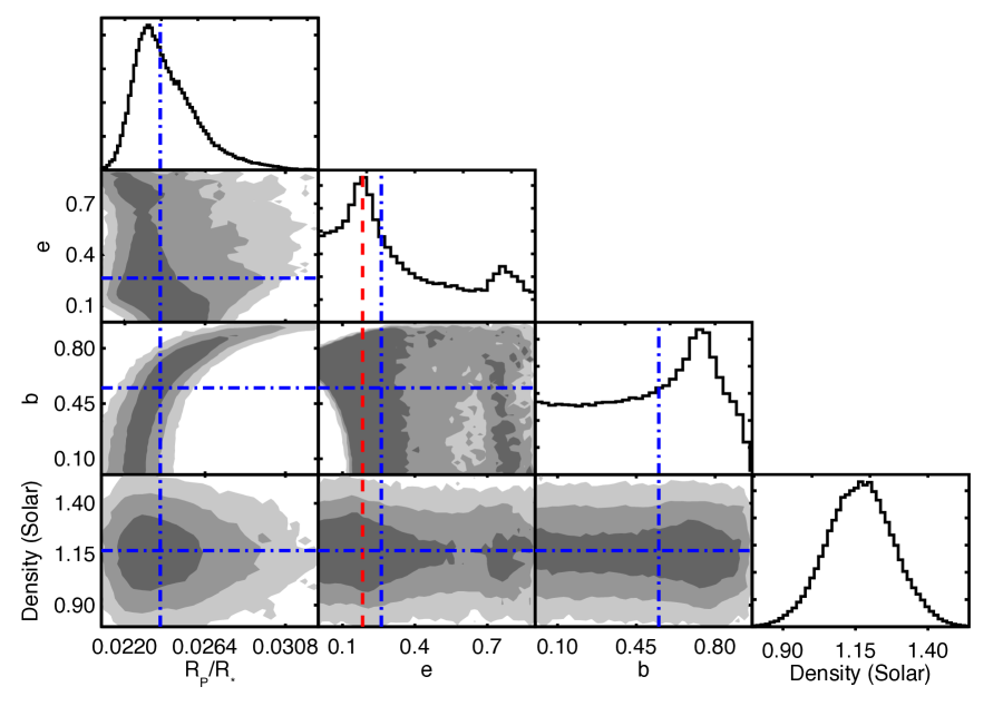
Figure 2: Results of the ZEIT MCMC transit-fitting procedure. This corner plot shows posterior distributions and correlations of a subset of the transit-fit parameters, including the ratio of planetary-to-stellar radius $R_{p}/R_{\star}$, eccentricity $e$, impact parameter $b$, and stellar density in solar units. The blue lines indicate the median values for each distribution; the red line shows the mode for the eccentricity plot. The shaded regions mark the 68%, 95%, and 99.7% contours of the MCMC posteriors.

3 Properties of the host star

Curtis et al. (2013) demonstrated that K2-231 is a member of Ruprecht 147, and therefore it should share the properties common to the cluster, including a spectroscopic metallicity of [Fe/H] = +0.10 dex (Curtis, 2016), an an age of 3 Gyr, a distance of 295 pc based on the distance modulus of $m-M=7.35$, and an interstellar extinction of $A_{V}=0.25$ mag, derived from fitting Dartmouth isochrone models (Dotter et al., 2008) to the optical and NIR color–magnitude diagrams (CMDs). We estimate the mass and radius of this star with a combination of spectroscopic and photometric data and then argue that it is likely single (i.e., not a stellar binary).

3.1 Spectroscopy

On 2016 July 15, we used the MIKE spectrograph (Bernstein et al., 2003) on the 6.5 m Magellan Clay Telescope at Las Campanas Observatory in Chile to acquire a spectrum of K2-231 with the 0$\farcs$70 slit, corresponding to a spectral resolution of $R=42,000$; the per-pixel signal-to-noise ratio is $S/N=130$ and 208 at the peaks of the Mg I b and 5940–6100 Å orders, respectively. We also observed six other solar analogs in R147 at $R=42,000$ and 20 solar analogs in the field at $R=55,000$ (including 18 Sco and the Sun as seen from the reflection off of the dwarf planet Ceres, which we observed with both resolution settings). We reduced these spectra with the Carnegie Python pipeline (“CarPy”), which performs the standard calibrations (i.e., overscan, bias, flat-field, sky-background, and scattered-light corrections, and mapping in wavelength using thorium–argon lamp spectra).

We analyzed these spectra with version 423 of Spectroscopy Made Easy (SME; Valenti & Piskunov, 1996) following the Valenti & Fischer (2005) procedure. Adopting stellar properties for the field stars from Brewer et al. (2016), that sample spans $T_{\mbox{\scriptsize eff}}$ = 5579–5960 K, $\log g$ = 4.10–4.50 dex, and [Fe/H] = $-0.09$ to $+0.14$ dex. We find median offsets and standard deviations between the Brewer et al. (2016) properties and our values of $T_{\mbox{\scriptsize eff}}$ = $-11$, 27 K, $\log g$ = $-0.04$, 0.035 dex, and [Fe/H] = $-0.016$, 0.02 dex. These numbers illustrate our ability to reproduce the Brewer et al. (2016) results with different data and a different SME procedure (we do not employ the expanded spectral range and line list of Brewer et al., 2015, 2016), and they are all within the SME statistical uncertainties quoted by Valenti & Fischer (2005) of 44 K, 0.06 dex, and 0.03 dex, respectively.

Regarding the sample of seven solar analogs in R147, after applying the offsets, we find [Fe/H]$=+0.10\pm 0.04$ dex, While the R147 dispersion is higher than that measured in the field star sample relative to the Brewer et al. (2016) metallicities, this is probably due to the typically lower $S/N$s and spectral resolutions of the R147 spectra (the stars are much fainter) compared to the field stars taken from Brewer et al. (2016), and not intrinsic to the sample.

For a separate project, Iván Ramírez measured stellar properties for five of these solar analogs with the same or similar MIKE spectra (since his work, we have collected higher-quality data for particular stars for our analysis described here). Following Ramírez et al. (2013), he employed a differential analysis with respect to the Sun by enforcing the excitation/ionization balance of iron lines using the MOOG spectral synthesis code. He also fit the telluric-free regions of the wings of H$\alpha$ using the Barklem et al. (2002) grid. For the same project, Luca Casagrande measured IRFM temperatures for these stars following Casagrande et al. (2010). For these five stars, we find a median offset and standard deviation for our SME values minus theirs of $-26\pm 29$ K for the Fe method, $-4\pm 22$ K for H$\alpha$, and $-31\pm 73$ K for IRFM (I. Ramírez & L. Casagrande 2013, private communication). These differences are all within the uncertainties quoted and cross-validate our adopted temperature scale.

Based on our results for the field star sample, the R147 members, and the SME statistical uncertainties quoted by Valenti & Fischer (2005), we adopt the following spectroscopic parameter precisions: 50 K for $T_{\mbox{\scriptsize eff}}$, 0.06 for $\log g$, and 0.04 dex for [Fe/H]. Our error analysis assumes that our uncertainties are limited by the data quality and our analysis technique, and not systematics inherent in the models. As our sample is comprised of stars quite similar to the Sun, the issues that tend to plague analyses of non-solar-type stars are assumed to be largely mitigated. The procedure accurately reproduces the Sun’s properties by design, as the line data were tuned to the solar spectrum; therefore, we assume that it can safely be applied to solar twins with the same degree of accuracy, and we adopt our precision estimates as our total parameter uncertainties.

For K2-231, we found an effective temperature of $T_{\mbox{\scriptsize eff}}$ = 5697 K, surface gravity of $\log g$ = 4.453 dex, iron abundance of [Fe/H] = +0.141 dex, and rotational broadening of $v\sin i$ = 1.95 $\mbox{km s}^{-1}$ when we adopted the macroturbulence relation from Valenti & Fischer (2005) (i.e., $v_{\rm mac}=3.87$ $\mbox{km s}^{-1}$). Adopting our preferred parameters for the Dartmouth isochrone model to describe the R147 cluster (age of 3 Gyr and [Fe/H] = +0.1 dex) and querying the model at the spectroscopic temperature yields an isochrone-constrained surface gravity of $\log g=4.483$ dex, which we adopt for $\log g$. We refit the spectrum with metallicity fixed to the cluster value and $\log g$ fixed to this isochrone value, which returned $T_{\mbox{\scriptsize eff}}=5672$ K and $v\sin i=1.3$ $\mbox{km s}^{-1}$, which is only 25 K cooler than the unconstrained fit.

3.2 Stellar mass and radius

Table 2: Photometry for K2-231

Instrument	Band	mag	error	$A/A_{V}$
Gaia	$G$	12.46	$\cdots$	0.861
APASS	$B$	13.50	0.03	1.297
APASS	$V$	12.71	0.04	1.006
CFHT/MegaCam	$g^{\prime}$	13.02	0.02	1.167
APASS	$g$	13.07	0.01	1.206
CFHT/MegaCam	$r^{\prime}$	12.46	0.02	0.860
APASS	$r$	12.47	0.07	0.871
CFHT/MegaCam	$i^{\prime}$	12.27	0.02	0.656
APASS	$i$	12.26	0.04	0.683
2MASS	$J$	11.29	0.02	0.291
2MASS	$H$	11.00	0.03	0.184
2MASS	$K_{S}$	10.86	0.02	0.115
UKIRT/WFCAM	$J$	11.30	0.02	0.283
UKIRT/WFCAM	$K$	10.92	0.02	0.114
WISE	$W1$	10.75	0.02	0.071
WISE	$W2$	10.84	0.02	0.055

Note. — (1) Name of instrument or survey. (2) Photometric band/filter employed. (3,4) Magnitude and uncertainty for that observation, where pipelines/surveys quoted errors below 0.01 mag, we set the value to 0.02 mag for analysis. (5) Interstellar reddening coefficients computed by the Padova/PARSEC isochrone group (Bressan et al., 2012) for a G2V star using the Cardelli et al. (1989) extinction law and following a procedure similar to that described by Girardi et al. (2008).

We estimated the mass and radius of K2-231 by combining our spectroscopic results with the optical and NIR photometry provided in Table 2. We assembled photometry from Gaia (Gaia Collaboration et al., 2016a, b), the AAVSO Photometric All-Sky Survey (APASS; Henden et al., 2016) the CFHT’s MegaCam (Hora et al., 1994) presented by Curtis et al. (2013), the Two Micron All-Sky Survey (2MASS; Skrutskie et al., 2006), the United Kingdom Infra-Red Telescope’s (UKIRT) Wide Field Infrared Camera (WFCAM; Hirst et al., 2006) that was acquired by coauthor A.L. Kraus in 2011 and accessed from the WFCAM Science Archive, and NASA’s Wide-field Infrared Survey Explorer (WISE; Wright et al., 2010).

First, we used the PARAM 1.3 input form—the “web interface for the Bayesian estimation of stellar parameters” described by da Silva et al. (2006)—to estimate the mass and radius of the host star. This service uses the PARSEC stellar evolution tracks (version 1.1; Bressan et al., 2012). The procedure requires as input the effective temperature, metallicity, parallax, and $V$ magnitude. We adopted the Curtis et al. (2013) distance modulus and visual extinction to estimate the dereddened magnitude ($V_{0}=V-0.25=12.458$) and parallax of $\pi=3.39$ $\mbox{mas yr}^{-1}$ (calculated from 295 pc). For parameter uncertainties, we adopted 50 K and 0.05 dex for $T_{\mbox{\scriptsize eff}}$ and [Fe/H], and 0.05 mag for $V_{0}$ and 0.15 mas for parallax based on the uncertainty in $A_{V}$ and $m-M$. PARAM 1.3 returned age $t_{\star}=1.7\pm 1.6$ Gyr, mass $M_{\star}=1.009\pm 0.027$ $\mbox{M}_{\odot}$, $\log g_{\star}=4.474\pm 0.029$ dex (cgs), and radius $R_{\star}=0.934\pm 0.029$ $\mbox{R}_{\odot}$.

Next, we estimated the mass and radius using the Python isochrones package (Morton, 2015). We adopted the spectroscopic $T_{\mbox{\scriptsize eff}}$ and $\log g$ values, the cluster metallicity and parallax, and the de-reddened broadband photometry from Table 2, and ran the fit assuming the photometry was derived from a blended and physically associated binary. Only 56% of nearby field stars are single (Raghavan et al., 2010), so it is important to consider at least binarity when characterizing this system (Raghavan et al. also found that 11% of nearby stars are in $3+$ multiples). We used grid models from the Dartmouth Stellar Evolution Database (Dotter et al., 2008) and sampled the posteriors using MultiNest (Feroz & Hobson, 2008; Feroz et al., 2009, 2013) implemented in Python with the PyMultiNest package (Buchner et al., 2014). Expressing uncertainties as the 68.3% (1$\sigma$) confidence intervals of the posterior distributions, we found $M_{1}=1.013\pm 0.016$ $\mbox{M}_{\odot}$, $R_{1}=0.944\pm 0.021$ $\mbox{R}_{\odot}$, and $M_{2}=0.238\pm 0.104$ $\mbox{M}_{\odot}$.

If the host is indeed single, then we can expect the parallax-constrained photometric analysis to return a small secondary mass with a value at approximately the threshold where its contributed flux is on par with the photometric errors (i.e., consistent with no secondary). Based on this low secondary-mass estimate, there is no evidence from the photometry for a secondary companion: the difference in magnitude between the resulting primary and secondary stars is $\Delta V=7.29$ and $\Delta K=4.18$, which is too large of a contrast to detect from these data (i.e., the difference between the primary and the combined magnitude of both stars is 0.001 mag in $V$ and 0.023 mag in $K$, the latter of which is on par with the measurement errors). We reran the fit with isochrones assuming a single star, which returned $M_{\star}=1.004\pm 0.017$ $\mbox{M}_{\odot}$, $R_{\star}=0.938\pm 0.022$ $\mbox{R}_{\odot}$, $d=302\pm 8$ pc, $A_{V}=0.29\pm 0.05$, and $t=2.5\pm 1$ Gyr. The age, distance, and reddening values are consistent with the CMD isochrone fitting results from Curtis et al. (2013); the mass and radius is consistent with the PARSEC/PARAM result quoted above.

To further test possible systematics in the isochrone fitting methods and models, we derived stellar properties using the isoclassify code (Huber et al., 2017), conditioning spectroscopic $T_{\mbox{\scriptsize eff}}$, $\log g$, $[\mbox{Fe}/\mbox{H}]$, parallax, and 2MASS $JHK$ photometry on a grid of interpolated MIST isochrones (Dotter, 2016). This returned $M_{\star}=1.014+0.021-0.022$ $\mbox{M}_{\odot}$, $R_{\star}=0.960+0.027-0.024$ $\mbox{R}_{\odot}$, $d=309+9-9$ pc, $A_{V}=0.09+0.27-0.24$ mag, and $t=2.3+1.6-1.3$ Gyr, in excellent agreement with the values derived from other isochrone models and methods.

Again, systematic uncertainties in the models are likely negligible due to the Sun-like nature of the host star (whereas, for example, K-dwarf models are known to diverge between PARSEC and Dartmouth; Huber et al., 2016; Curtis et al., 2013). The dispersion in masses and radii derived from the three isochrone models are well within the uncertainties returned by each method, so we adopt the maximum uncertainties from the various experiments as our final measurement uncertainties and we take the mean as our final values: $M_{\star}=1.009\pm 0.027$ $\mbox{M}_{\odot}$ and $R_{\star}=0.945\pm 0.027$ $\mbox{R}_{\odot}$.

According to the MIST model, a 3 Gyr star with mass $M_{\star}=1.009$ $\mbox{M}_{\odot}$ and [Fe/H] = +0.1 dex has $T_{\mbox{\scriptsize eff}}$ = 5695 K. This value is only 2 K cooler than our SME result, and so we adopt this value as the effective temperature of this star.

3.3 K2-231 Is Likely Single

Photometry: Reiterating our result from the previous subsection, modeling the broadband photometry with the isochrones package suggests that K2-231 does not have a companion with a mass $M_{2}>0.34$ $\mbox{M}_{\odot}$.

Adaptive optics imaging and coronagraphy: We acquired natural guide star AO imaging in $K^{\prime}$ ($\lambda=2.124~{}\mu$m) with NIRC2 on the Keck II telescope. We also used the “corona600” occulting spot, which has a diameter of 600 mas and an approximate transmission of 0.22% in $K^{\prime}$. The observations were acquired, reduced, and analyzed following Kraus et al. (2016). Table 3 lists the $K^{\prime}$ detection limits as a function of angular separation from K2-231 ranging from 150 to 2000 mas.

Table 4 lists six stars within $8^{\prime\prime}$ that were detected, including coordinates; angular separation, position angle, and $K^{\prime}$ contrast relative to K2-231; and photometry from Gaia, CFHT/MegaCam, and UKIRT/WFCAM. This table also lists four stars within $10^{\prime\prime}$ detected in the UKIRT imaging that were missed by NIRC2. Figure 3 shows a $30^{\prime\prime}$-square $K$-band image from UKIRT/WFCAM centered on the host star and highlights the noncoronagraphic imaging footprint (magenta dashed line); note that we had to offset the pointing after the first image in order to get the bright neighboring star onto the detector, which is why there is effectively a double footprint. For reference, two circles with radii of 5$\farcs$5 and $9^{\prime\prime}$ are also overlaid to show the approximate extraction apertures used to produce light-curves from the K2 data. The AO imaging and coronagraphy yielded six detections, four of which were matched in the UKIRT imaging (red circles), and two of which were apparently fainter than the UKIRT source catalog limit (blue circles), but nevertheless show up in the image. Due to the placement, size, and orientation of the NIRC2 footprint, four stars within $10^{\prime\prime}$ of the host were missed but show up in WFCAM (cyan circles).

We calculated proper motions for the eight stars that matched in both Gaia and either or both MegaCam and WFCAM and found that none but the final entry appear comoving with R147. We also inspected optical and NIR CMDs with the cluster Dartmouth model overlaid and noted that stars 1, 3, 8, and 9 are inconsistent with membership, whereas 6, 7, and 10 appear near but beyond the base of the Dartmouth isochrone. As 6 and 7 appear to be ruled out by their discrepant proper motions, this leaves 10 as the sole candidate member in this list. Although too faint for Gaia, it is conceivable that we could measure its proper motion with additional NIRC2 images in the future: the uncertainty on $\rho$ is under 5 mas, whereas R147 moves at $-28$ $\mbox{mas yr}^{-1}$ in declination, so two observations spaced approximately by one year should clearly reveal any comoving stars while canceling out the parallax effect.

Only two stars are detected within 5$\farcs$5, which is the radius of the smallest circular moving aperture that we used to extract light-curves. One star is near the edge of this radius and is nearly 480 times fainter than K2-231. The other, at 4$\farcs$2 southward, is 40 times fainter, and we consider it our primary false-positive source.

These constraints are illustrated in Figure 4 by the dark blue shading, which covers the majority of the upper right region. Masses/contrasts below the hydrogen-burning limit at $\sim$0.07 $\mbox{M}_{\odot}$ are shaded gray and found below the black horizontal line toward the bottom of the figure, which the AO limit reaches at $\sim$700 mas—this depth is not only important for searching for stellar binaries, but also for identifying faint, unassociated stars in the background. The lowest mass star represented in the Dartmouth isochrone model is $M\approx 0.12$ $\mbox{M}_{\odot}$: we also shade this region gray and label it “VLM” for “very low mass star” to distinguish it from the region below the substellar boundary while highlighting that this represents a small region of the secondary mass parameter space compared to the top-half of the figure.

Keck/NIRC2 aperture-masking interferometry: We also acquired nonredundant aperture-masking interferometry data for K2-231 on 2017 June 22 in natural guide star mode, along with EPIC 219511354 for calibration. For the target and reference star, we obtained four (three) interferograms for a total of 80 (60) s on EPIC 219800881 (EPIC 219511354), which we analyzed following Kraus et al. (2008, 2011, 2016). We report no detections within the limits quoted in Table 5. These constraints are illustrated in Figure 4 by the red shaded region, which is drawn according to the midpoints of the angular separation ranges listed in Table 5.

Table 3: Keck/NIRC2 Imaging Detection Limits

MJD	Filter +	Number of	Total	Contrast Limit ($\Delta K^{\prime}$ in mag) at Projected Separation ($\rho$ in mas)
	Coronagraph	Frames	Exposure (s)	150	200	250	300	400	500	700	1000	1500	2000
57933.42	$K^{\prime}$	6	120.00	4.9	6.0	6.4	6.6	7.3	7.9	8.6	8.8	8.9	8.9
57933.43	$K^{\prime}$+C06	4	80.00	$\cdots$	$\cdots$	$\cdots$	$\cdots$	7.2	7.2	7.9	9.3	9.7	9.8

Note. — The second entry is for the coronagraphic imaging observations, which obstructs the inner 3 mas radius.

Table 4: Keck/NIRC2 and UKIRT/WFCAM Detected Neighbors

#	R.A.	Decl.	$\rho$	PA	$\Delta K^{\prime}$	$G$	$g^{\prime}$	$r^{\prime}$	$i^{\prime}$	$J$	$K$
	J2000	J2000	(mas)	(deg)	(mag)	(mag)	(mag)	(mag)	(mag)	(mag)	(mag)
1	19:16:22.005	$-$15:46:20.58	4179.9 $\pm$ 1.7	186.488 $\pm$ 0.023	4.032 $\pm$0.003	16.52	17.12	16.46	16.24	15.18	14.76
2	19:16:22.319	$-$15:46:19.68	5182.3 $\pm$ 2.0	129.033 $\pm$ 0.021	6.708 $\pm$0.017	18.84	$\cdots$	$\cdots$	$\cdots$	17.66	17.25
3	19:16:22.424	$-$15:46:13.21	6429.6 $\pm$ 2.4	60.404 $\pm$ 0.020	7.243 $\pm$0.117	$\cdots$	$\cdots$	$\cdots$	$\cdots$	18.92	18.27
4	19:16:22.118	$-$15:46:23.57	7388.2 $\pm$ 3.8	170.104 $\pm$ 0.029	8.216 $\pm$0.064	$\cdots$	$\cdots$	$\cdots$	$\cdots$	$\cdots$	$\cdots$
5	19:16:22.551	$-$15:46:16.51	7693.7 $\pm$ 4.4	91.145 $\pm$ 0.032	8.521 $\pm$0.076	$\cdots$	$\cdots$	$\cdots$	$\cdots$	$\cdots$	$\cdots$
6	19:16:22.269	$-$15:46:23.41	7739.2 $\pm$ 2.3	154.535 $\pm$ 0.015	6.677 $\pm$0.015	20.06	22.86	20.81	20.11	17.99	17.18
7	19:16:21.649	$-$15:46:13.25	6585.7	297.421	$\cdots$	$\cdots$	23.48	21.73	20.71	18.01	17.21
8	19:16:21.807	$-$15:46:09.67	7466.9	332.356	$\cdots$	$\cdots$	21.05	20.64	20.13	18.75	18.46
9	19:16:21.821	$-$15:46:07.48	9386.6	339.730	$\cdots$	18.896	19.07	18.62	18.32	17.54	17.06
10	19:16:21.439	$-$15:46:20.08	9760.9	247.148	$\cdots$	$\cdots$	24.31	23.47	21.71	18.94	18.17

Note. — The third object was only detected in the coronagraphic observation because it fell on the edge of the NIRC2 imaging footprint; see Figure 3. The objects in the lower section were detected with UKIRT but missed by NIRC2 due to the placement, size, and orientation of the NIRC2 field. Star 10 is the only neighbor that appears co-moving with R147 (and therefore the planet host; stars 4 and 5 were only detected in NIRC2 and so lack a second astrometric epoch needed to calculate proper motions), with a CFHT$-$UKIRT proper motion of $(\mu_{\alpha}\cos\delta,\mu_{\delta})=(3,-31)$ $\mbox{mas yr}^{-1}$, although the baseline is relatively short at $\sim$3 years and we have not quantified the accuracy or precision with tests of anything near that faint.

Table 5: Keck/NIRC2 aperture-masking interferometry detection limits

Confidence	MJD	Contrast Limit ($\Delta K^{\prime}$ in mag) at Projected Separation ($\rho$ in mas)
Interval		10-20	20-40	40-80	80-160	160-240	240-320
99.9%	57933.4	0.06	3.02	4.02	3.79	3.19	1.96
99% only	57933.4	0.26	3.24	4.20	3.97	3.42	2.2

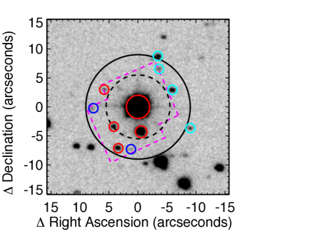
Figure 3: Image of K2-231 and neighboring stars from UKIRT/WFCAM, taken in 2011. The solid black circle shows the $9^{\prime\prime}$ radius aperture used to extract the light-curve. The dashed black circle has a radius of $5.5^{\prime\prime}$ and is the smallest aperture we tested; the transits are still visible, which means that the object is either transiting K2-231 or the fainter star 4^′′ southward. The dashed magenta line traces out the Keck II NIRC2 footprint: six stars were detected, four of which cross-matched with the UKIRT catalog (red) and two of which were apparently too faint, though they show some signal in the image (blue). Four other stars are detected in the WFCAM image within 10^′′ but were missed by NIRC2 due to the size, placement, and orientation of the field (cyan). Properties of these 10 neighboring stars are listed in Table 4.

Spectroscopy: We observed K2-231 on 2017 June 2 (near quadrature, according to the transit ephemeris) with the High Resolution Echelle Spectrometer (HIRES; Vogt et al., 1994) on the 10 m telescope at Keck Observatory. No secondary spectral lines were found down to 1% of the brightness of the primary ($\sim$0.49 $\mbox{M}_{\odot}$; already ruled out by photometric modeling), excluding the range of under $\pm$10 $\mbox{km s}^{-1}$ separation from the primary (Kolbl et al., 2015).

RV variability: We collected RVs every few years beginning in 2007, which show no trend due to a stellar companion over the baseline of nearly ten years. These include observations with the Lick/Hamilton and MMT/Hectochelle spectrographs presented in Curtis et al. (2013), the HIRES spectrum mentioned above (Chubak et al., 2012), and the Magellan/MIKE spectra discussed earlier.

Separately, a team led by PI Minniti targeted R147 with the High Accuracy Radial velocity Planet Searcher (HARPS; Mayor et al., 2003) in 2013-2014 to look for exoplanets in R147 with masses greater than or approximately equal to Neptune in relatively short-period orbits and acquired six RV epochs with individual precisions of $\approx$10 $\mbox{m s}^{-1}$. Data were reduced and RVs extracted with the HARPS Data Reduction Software. We downloaded the reduced data, including the pipeline RVs and uncertainties, from the ESO archive.

We recalculated the RVs for the Lick 2007, Hecto 2010, and MIKE 2016 epochs differentially relative to the solar-twin member CWW 91 (NID 0739-0790842; EPIC 219698970). They were observed concurrently (Hectochelle) or close in time on the same night, with the RV zero point of the reference star set to its median HARPS RV of $41.654\pm 0.014$ $\mbox{km s}^{-1}$ (five visits over 1.9 yr). For reference, Curtis et al. (2013) reported a HIRES epoch of 41.5 $\mbox{km s}^{-1}$ for this reference star. CWW 91 was not observed on the same run for the MIKE 2012 epoch, so instead we calculated the zero point with six other stars with HARPS RVs with concurrent MIKE observations in order to mitigate the effect of any one of those stars being an unknown binary. We note that this epoch happens to be the largest outlier, although consistent within the estimated uncertainty for our MIKE RVs.

The RVs are provided in Table 6. Averaging the two Hectochelle RVs, as well as the six HARPS RVs, yields six individual RV epochs spanning 9.8 yr with an unweighted rms of 250 $\mbox{m s}^{-1}$. The HARPS RV rms is 6 $\mbox{m s}^{-1}$ over 10 months.

Table 6: RVs for K2-231

Date	MJD = JD	RV	Uncertainty	Observatory
	$-2,400,000$	($\mbox{km s}^{-1}$)	($\mbox{km s}^{-1}$)
2007 Aug 23	54335.789	41.584	1.00	Lick
2010 Jul 05	55382.264	41.397	0.30	Hecto
2010 Jul 06	55383.269	41.377	0.30	Hecto
2012 Sep 30	56200.644	42.112	0.70	MIKE
2013 Aug 10	56514.247	41.580	0.012	HARPS
2014 May 07	56784.386	41.586	0.008	HARPS
2014 May 08	56785.399	41.573	0.007	HARPS
2014 May 09	56786.404	41.574	0.007	HARPS
2014 May 27	56804.311	41.570	0.016	HARPS
2014 Jun 22	56830.298	41.577	0.008	HARPS
2016 Jul 15	57584.743	41.550	0.70	MIKE
2017 Jun 02	57907.075	41.760	0.30	HIRES
Star B:
2017 Jun 08	57913.062	$-24.92$	0.20	HIRES
2017 Aug 28	57993.804	$-25.28$	0.20	HIRES

Note. — RV measurements collected over nearly ten years, with rms = 250 $\mbox{m s}^{-1}$, consistent with K2-231 being single. See Section 3.3 for details.

Figure 4: Constraints on binary companionship for hypothetical secondaries with $K^{\prime}$-band contrast (left) or stellar mass ($\mbox{M}_{\odot}$; right) as a function of projected separation in angular units (mas; bottom) or physical units (AU; top). At separations of $\rho>200$ mas, the NIRC2 AO imaging and coronagraphy (dark blue lined region) probe deeper than the very low mass stars and reaches down to the hydrogen-burning limit at $\sim$700 mas (gray shaded region), which is useful for searching for background blends; the NIRC2 non-redundant masking data reach closer to the primary star, but not quite as deep (red shaded region). Modeling the broadband photometry with isochrones rules out secondaries of any separation with masses greater than $M_{2}\gtrsim 0.34$ $\mbox{M}_{\odot}$ (light blue shaded region). Combining these various constraints leaves a small region of parameter space under 45 AU (projected) for systems with $M_{2}\lesssim 0.34$ $\mbox{M}_{\odot}$. The precise HARPS RVs can rule out much of this remaining parameter space for edge-on orbits (green shaded region); accounting for possible inclination of the binary orbital plane relative to the primary–planet orbit will restrict this to smaller separations.

4 Planet Validation

First, we inspected the six individual transits for variations in depth, timing, and duration between the odd and even events that would indicate eccentricity or dissimilar stellar companions, under the assumption that these are stellar eclipsing binary (EB) transits. Figure 5 shows each transit event separately, along with the EXOFAST transit model, and they are all consistent with the model and each other.

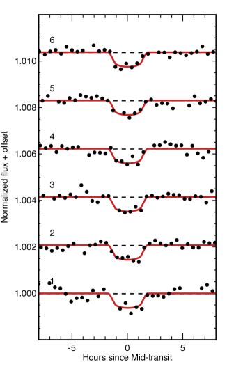
Figure 5: Individual transit events along with the EXOFAST transit model for K2-231 b. Their consistency, especially between odd- and even-numbered events, indicates that they are due to either the same transiting object or two with negligible differences in a circular orbit (i.e., an equal-mass EB).

One might think that the cluster environment would create a crowded field that would complicate the photometric analysis. In fact, R147 is relatively sparse due to both the low number of (confirmed) members ($N\approx 150$) and closer distance compared to clusters like NGC 6811 (295 pc versus $\sim$1100 pc). However, R147’s location in the Galactic plane near Sagittarius ($l=21^{\circ},b=-13^{\circ}$) means that there are quite a few background stars. We opted for a circular moving aperture to track K2-231’s motion across its individual aperture while excluding as many of the background stars shown in Figure 3 as possible. The aperture used to produce the EVEREST light-curve that we used to identify the transiting planet contained all the bright stars shown to the southwest of K2-231. Our 9^′′ circular aperture excludes all but one of these brighter stars. We also created apertures as small as 5$\farcs$5 (1.39 pixels) to reject many of the fainter stars, and the transit depth appears the same as in the larger apertures, meaning that we can attribute the transit to either of the two stars encircled by the dashed line in the figure.

4.1 Star B: The Bright Neighbor

The star that remains blended is located approximately 4$\farcs$2 south of K2-231, and we refer to this star as “star B.” The mean difference in the various photometric bands shows it to be 3.98 mag fainter than K2-231 (neglecting differences in interstellar reddening). The Gaia and CFHT/MegaCam epochs are separated by $\sim$6.5 years, which is enough to calculate proper motions to test for association with R147, given the cluster’s relatively large proper motion in declination of $\mu_{\delta}=-28$ $\mbox{mas yr}^{-1}$. For K2-231, we measure $\mu_{\delta}=-25.6$ $\mbox{mas yr}^{-1}$, and for star B, we find $\mu_{\delta}=-9.4$ $\mbox{mas yr}^{-1}$, which does not support cluster membership.

We can also model the CFHT and UKIRT photometry with isochrones under the assumption that it is a single dwarf star by applying a Gaussian prior on $\log g=4.4\pm 0.5$, and we find a mass $M=1.06-0.10+0.13$ $\mbox{M}_{\odot}$, radius $R=1.013-0.16+0.19$ $\mbox{R}_{\odot}$, distance $d=2204-343+406$ pc, and visual extinction $A_{V}=0.63\pm 0.18$ mag.

The 3D Galactic dust map produced from 2MASS and Pan-STARRS 1 (Green et al., 2015) toward K2-231 quotes an interstellar reddening at 300 pc (the approximate distance to R147) of $E(B-V)=0.07+0.03-0.04$ (i.e., $A_{V}=0.22+0.09-0.12$, which is consistent with the value we find from CMD isochrone fitting). According to this map, interstellar reddening is $E(B-V)=0.16\pm 0.02$ or $A_{V}=0.50\pm 0.06$ at 2.2 kpc, the distance we infer for star B, and reaches a maximum value of $E(B-V)=0.17\pm 0.02$ at 2.28 kpc ($A_{V}=0.53$). This value is consistent with our result from isochrones due to the large uncertainty, which is compounded when considering our assumption of singularity and a dwarf luminosity class. The Schlegel et al. (1998) dust map value is marginally less at $E(B-V)=0.146$ or $A_{V}=0.45$, and the recalibrated map from Schlafly & Finkbeiner (2011) quotes $E(B-V)=0.125$ or $A_{V}=0.39$.

The proper motions and stellar properties are inconsistent with membership, meaning that star B is likely a background star. A quick test with BLENDER (described in the next section; Torres et al., 2011a) indicates that the broad features of the transit light-curve can indeed be fit reasonably well if star B is a background EB. Assuming that both the target and star B are solar-mass stars, we find a decent fit for a companion to star B of about 0.26 $\mbox{M}_{\odot}$. This EB produces a secondary eclipse, but it is very shallow ($\sim$30 ppm) and is probably not detectable in the data, given the typical scatter of $\sim$120 ppm. If we resolved star B, we expect that the undiluted transit due to this hypothetical EB would be $\sim$2.5% , which could be detected from ground-based photometric observations in and out of transit. We attempted to conduct such observations with the Las Cumbres Observatory, but were unable to acquire the relevant data.

Assuming a circular orbit, the RV semi-amplitude of such a hypothetical single-lined EB is 19.8 $\mbox{km s}^{-1}$, which is also feasible to test and rule out with a few RV observations. We acquired two RV epochs of star B with HIRES, which were taken 7.37 and 9.93 days from midtransit (propagated forward according to the transit ephemeris in Table 1), near the secondary eclipse and second quadrature points at phases of 0.53 and 0.72, respectively. The RVs, listed at the bottom of Table 6, are constant to within their 0.2 $\mbox{km s}^{-1}$ uncertainties. Furthermore, these HIRES spectra have sufficient quality to rule out secondary spectral lines down to 1% of the brightness of the primary, excluding $\pm$10 $\mbox{km s}^{-1}$ separation (Kolbl et al., 2015). This rules out the false-positive scenario where star B is a background EB.

4.2 False-alarm Probability

Having excluded the only visible neighboring star within the aperture as the source of the transit signal, we then examined the likelihood of a false positive caused by unseen stars. For this, we applied the BLENDER statistical validation technique (Torres et al., 2004, 2011b, 2015) that has been used previously to validate candidates from the Kepler mission (see, e.g., Torres et al., 2017; Fressin et al., 2012; Borucki et al., 2013; Barclay et al., 2013; Meibom et al., 2013; Kipping et al., 2014, 2016; Jenkins et al., 2015). For full details of the methodology and additional examples of its application, we refer the reader to the first three sources above. Briefly, BLENDER models the light-curve as a blend between the assumed host star and another object falling within the photometric aperture that may be an EB or a star transited by a larger planet, such that the eclipse depths from these sources would be diluted by the brighter target to the point where they mimic shallow planetary transits. These contaminants may be in either the background or foreground of the target or physically associated with it. Fits to the K2 light-curves of a large number of such simulated blend models with a broad range of properties allows us to rule many of them out that result in poor fits, and Monte Carlo simulations conditioned on constraints from the follow-up observations (high-resolution spectroscopy, imaging, RVs, color information) yield a probability of 99.86% that the candidate is a planet, as opposed to a false positive of one kind or another. Thus, we consider K2-231 b to be statistically validated as a planet.

5 Discussion

We have demonstrated that K2-231 is a single, solar twin member of the 3 Gyr open cluster Ruprecht 147 and that it hosts a statistically validated sub-Neptune exoplanet in a 13.84 day orbit.

5.1 Expected yield

5.2 Comparison to field stars

Fulton et al. (2017) showed that the distribution of planetary radii is bimodal, with a valley at about 1.8 $\mbox{R}_{\earth}$ and a peak at the larger side at 2.4 $\mbox{R}_{\earth}$ representing sub-Neptunes, which they argued are a different class of planets than the super Earths found on the smaller side of the gap (see their Figure 7). With a radius of $\sim$2.5 $\mbox{R}_{\earth}$, K2-231 b falls on the large side of the planet radius gap (see also Rogers, 2015; Weiss & Marcy, 2014). Our Figure 6 presents a modified version of the bottom panel of Figure 8 from Fulton et al. (2017), which shows the completeness-corrected, two-dimensional distribution of planet size and orbital period derived from the Kepler sample. Our figure compares this distribution to the properties of K2-231 b and shows that it is found near a relative maximum. In other words, K2-231 b appears to have a fairly typical radius for a short-period ($P<29$ days) planet.

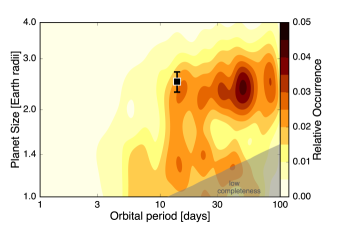
Figure 6: Two-dimensional distribution of planet size and orbital period found in the Kepler field, adopted from Fulton et al. (2017), is shown along with the location of K2-231 b. Restricting this distribution to periods less than 40 days (i.e., demanding the presence of two transits for a planet detection) means that K2-231 b is found near a relative maximum in this distribution.

5.3 Comparison to the NGC 6811 planets

Meibom et al. (2013) concluded that the frequency of planets discovered in the 1 Gyr Kepler cluster NGC 6811 is approximately equal to the Fressin et al. (2013) field rates based on two planets found out of 377 members surveyed. This is about half of the raw rate found in R147 (i.e., 1 in 100 versus 2 in 377); in other words, the same order of magnitude.

The two planets found in NGC 6811 are quite similar to K2-231 b: they are sub-Neptunes with radii of 2.8 and 2.94 $\mbox{R}_{\earth}$ and periods of 17.8 and 15.7 days (Kepler-66 b and 67 b, respectively). This is unlikely to be a mere coincidence, but as Figure 6 illustrates, planets with these approximate properties are relatively more prevalent. However, that figure shows that the relative occurrence of the sub-Neptunes continues, and even increases, to longer orbital periods. While the duration of the K2 survey of R147 was not long enough to identify planets in the 40–100 day regime, presumably such planets could have been found in NGC 6811 during the Kepler prime mission. With this limited sample, it is unclear if any meaning should be drawn from this regarding possible planetary architectures that can form and survive in a dense cluster, but it is at the very least an intriguing option to consider. However, we think this is probably due to the relatively lower $S/N$ light-curves due to NGC 6811’s large distance modulus and the reduction in transit depth and probability with increasing orbital period.

5.4 Similar planets and estimating the mass

Considering the planets with measured masses and radii in the field, there are currently five listed on exoplanets.org with $2.4<R_{p}/\mbox{R}_{\earth}<2.7$, $K>1$ $\mbox{m s}^{-1}$, and $P>5$ days: Kepler’s 96 b, 106 c and e, 131 b, and HIP 116454 b. The basic transit and physical properties of K2-231 b and its host are similar to those of Kepler 106 c: $M_{\star}=1.0$ $\mbox{M}_{\odot}$, [Fe/H]$=-0.12$ dex, $T_{\mbox{\scriptsize eff}}=5860$ K, $\log g=4.41$ dex, $V=13$, $P_{orb}=13$ days, $R_{P}=2.5$ $\mbox{R}_{\earth}$, and $a=0.111$ AU. Importantly, the RV semi-amplitude for Kepler 106 c is $K=2.71$ $\mbox{m s}^{-1}$, and the planet mass is $M_{p}=10.4$ $\mbox{M}_{\earth}$(Marcy et al., 2014), and this mass was measured with RV observations made with Keck/HIRES.

Applying the Wolfgang et al. (2016) mass–radius relation for sub-Neptune transiting planets (i.e., $R_{P}<4$ $\mbox{R}_{\earth}$), where $M/\mbox{M}_{\earth}=2.7(R/\mbox{R}_{\earth})^{1.3}$, predicts a mass for K2-231 b of $M_{p}\sim 8.75\pm 0.9\pm 1.9$ $\mbox{M}_{\earth}$, where the uncertainties represent the standard deviation of masses computed from a normally distributed sample of radii $R_{p}=2.5\pm 0.2$ $\mbox{R}_{\earth}$ and the normally distributed dispersion in mass of the relation, respectively. The Chen & Kipping (2017) probabilistic mass–radius relation, implemented with the Forecaster Python code, yields $M_{p}=7.2+5.1-3.1$ $\mbox{M}_{\earth}$. Assuming a circular orbit, Kepler’s Law predicts an RV semi-amplitude for K2-231 of $K\approx 2\pm 1$ $\mbox{m s}^{-1}$ in this mass range. K2-231 b would then become the first planet with a measured mass and density in an open cluster.

Appendix A Planets discovered in open clusters

Table A lists the 23 planets and three candidates that have been discovered to date in open clusters. We list KIC or EPIC IDs when available, whether the planet was discovered via transit or RV techniques (no cluster exoplanet has yet been characterized with both techniques), the $V$ magnitude and type of host, the orbital period, the planetary radius or mass ($m\,\sin\,i$), citations, and additional notes (e.g., “HJ,” referring to hot Jupiter). We assembled this list to determine how many planets are currently known in clusters, then decided that it might be of use and interest to the reader, so we provide it here.

Table A1: Planets in Clusters

Planet	KIC/EPIC	Discovery	$V$		Period	Radius /	Host	Notes	Citations
ID	ID	Method	(mag)		(days)	$M\sin i$	Info.
Pleiades (130 Myr):
$\cdots$	C4	$\cdots$	$\cdots$	$\cdots$	$\cdots$	$\cdots$	None found	6
Hyades (650 Myr):
$\epsilon$ Tau b	210754593	RV	3.53	594.9	7.6 $\mbox{M}_{\rm Jup}$	2.7 $\mbox{M}_{\odot}$ Giant	1st ever	19
HD 285507 b	210495452	RV	10.47	6.09	0.917 $\mbox{M}_{\rm Jup}$	K4.5	Eccentric HJ	18
K2-25 b	210490365	Tr	15.88	3.485	3.43 $\mbox{R}_{\earth}$	M4.5	$\cdots$	5, 10
K2-136-A b	247589423	Tr	11.20	7.98	0.99 $\mbox{R}_{\earth}$	K5.5	Stellar binary	4, 12
K2-136-A c	247589423	Tr	11.20	17.31	2.91 $\mbox{R}_{\earth}$	K5.5	Stellar binary	4, 12
K2-136-A d	247589423	Tr	11.20	25.58	1.45 $\mbox{R}_{\earth}$	K5.5	Stellar binary	4, 12
HD 283869 b	248045685	Tr	10.60	$\sim$106	1.96 $\mbox{R}_{\earth}$	K5	Candidate (1 transit)	20
Praesepe (650 Myr):
Pr0201 b	211998346	RV	10.52	4.43	0.54 $\mbox{M}_{\rm Jup}$	late-F	HJ, “two b’s”	17
Pr0211 b	211936827	RV	12.15	2.15	1.844 $\mbox{M}_{\rm Jup}$	late-G	HJ, “two b’s”	17
Pr0211 c	211936827	RV	12.15	$>$3500	7.9 $\mbox{M}_{\rm Jup}$	late-G	Eccentric; 1st multi	9
K2-95 b	211916756	Tr	17.27	10.14	3.7 $\mbox{R}_{\earth}$	0.43 $\mbox{M}_{\odot}$	$\cdots$	7, 11, 14, 15
K2-100 b	211990866	Tr	10.373	1.67	3.5 $\mbox{R}_{\earth}$	1.18 $\mbox{M}_{\odot}$	$\cdots$	1, 7, 11, 16
K2-101 b	211913977	Tr	12.552	14.68	2.0 $\mbox{R}_{\earth}$	0.80 $\mbox{M}_{\odot}$	$\cdots$	1, 7, 11, 16
K2-102 b	211970147	Tr	12.758	9.92	1.3 $\mbox{R}_{\earth}$	0.77 $\mbox{M}_{\odot}$	$\cdots$	11
K2-103 b	211822797	Tr	14.661	21.17	2.2 $\mbox{R}_{\earth}$	0.61 $\mbox{M}_{\odot}$	$\cdots$	11
K2-104 b	211969807	Tr	15.770	1.97	1.9 $\mbox{R}_{\earth}$	0.51 $\mbox{M}_{\odot}$	$\cdots$	7, 11
EPIC 211901114 b	211901114	Tr	16.485	1.65	9.6 $\mbox{R}_{\earth}$	0.46 $\mbox{M}_{\odot}$	Candidate	11
NGC 2423 (740 Myr):
TYC 5409-2156-1 b	$\cdots$	RV	9.45	714.3	10.6 $\mbox{M}_{\rm Jup}$	Giant	$\cdots$	8
NGC 6811 (1 Gyr):
Kepler-66 b	9836149	Tr	15.3	17.82	2.80 $\mbox{R}_{\earth}$	1.04 $\mbox{M}_{\odot}$	$\cdots$	13
Kepler-67 b	9532052	Tr	16.4	15.73	2.94 $\mbox{R}_{\earth}$	0.87 $\mbox{M}_{\odot}$	$\cdots$	13
Ruprecht 147 (3 Gyr):
K2-231 b	219800881	Tr	12.71	13.84	2.5 $\mbox{R}_{\earth}$	Solar twin	$\cdots$	This work
M67 (4 Gyr):
YBP 401 b	$\cdots$	RV	13.70	4.087	0.42 $\mbox{M}_{\rm Jup}$	F9V	HJ	2, 3
YBP 1194 b	211411531	RV	14.68	6.960	0.33 $\mbox{M}_{\rm Jup}$	G5V	HJ	2, 3
YBP 1514 b	211416296	RV	14.77	5.118	0.40 $\mbox{M}_{\rm Jup}$	G5V	HJ	2, 3
SAND 364 b	211403356	RV	9.80	121	1.57 $\mbox{M}_{\rm Jup}$	K3III	$\cdots$	2, 3
SAND 978 b	$\cdots$	RV	9.71	511	2.18 $\mbox{M}_{\rm Jup}$	K4III	Candidate	2, 3

References. — (1) Barros et al. (2016); (2) Brucalassi et al. (2014); (3) Brucalassi et al. (2017); (4) Ciardi et al. (2018); (5) David et al. (2016a); (6) Gaidos et al. (2017); (7) Libralato et al. (2016); (8) Lovis & Mayor (2007); (9) Malavolta et al. (2016); (10) Mann et al. (2016a); (11) Mann et al. (2017); (12) Mann et al. (2018); (13) Meibom et al. (2013); (14) Obermeier et al. (2016); (15) Pepper et al. (2017); (16) Pope et al. (2016); (17) Quinn et al. (2012); (18) Quinn et al. (2014); (19) Sato et al. (2007); (20) Vanderburg et al. (2018).

References

- Adams (2010) Adams, F. C. 2010, ARA&A, 48, 47
- Adams et al. (2006) Adams, F. C., Proszkow, E. M., Fatuzzo, M., & Myers, P. C. 2006, ApJ, 641, 504
- Altmann et al. (2017) Altmann, M., Roeser, S., Demleitner, M., Bastian, U., & Schilbach, E. 2017, A&A, 600, L4
- Barclay et al. (2013) Barclay, T., Burke, C. J., Howell, S. B., et al. 2013, ApJ, 768, 101
- Barklem et al. (2002) Barklem, P. S., Stempels, H. C., Allende Prieto, C., et al. 2002, A&A, 385, 951
- Barros et al. (2016) Barros, S. C. C., Demangeon, O., & Deleuil, M. 2016, A&A, 594, A100
- Bernstein et al. (2003) Bernstein, R., Shectman, S. A., Gunnels, S. M., Mochnacki, S., & Athey, A. E. 2003, in Proc. SPIE, Vol. 4841, Instrument Design and Performance for Optical/Infrared Ground-based Telescopes, ed. M. Iye & A. F. M. Moorwood, 1694
- Bonnell et al. (2001) Bonnell, I. A., Smith, K. W., Davies, M. B., & Horne, K. 2001, MNRAS, 322, 859
- Borucki et al. (2013) Borucki, W. J., Agol, E., Fressin, F., et al. 2013, Science, 340, 587
- Bressan et al. (2012) Bressan, A., Marigo, P., Girardi, L., et al. 2012, MNRAS, 427, 127
- Brewer et al. (2015) Brewer, J. M., Fischer, D. A., Basu, S., Valenti, J. A., & Piskunov, N. 2015, ApJ, 805, 126
- Brewer et al. (2016) Brewer, J. M., Fischer, D. A., Valenti, J. A., & Piskunov, N. 2016, ApJS, 225, 32
- Brucalassi et al. (2014) Brucalassi, A., Pasquini, L., Saglia, R., et al. 2014, A&A, 561, L9
- Brucalassi et al. (2016) —. 2016, A&A, 592, L1
- Brucalassi et al. (2017) Brucalassi, A., Koppenhoefer, J., Saglia, R., et al. 2017, A&A, 603, A85
- Buchner et al. (2014) Buchner, J., Georgakakis, A., Nandra, K., et al. 2014, A&A, 564, A125
- Cai et al. (2017) Cai, M. X., Kouwenhoven, M. B. N., Portegies Zwart, S. F., & Spurzem, R. 2017, MNRAS, 470, 4337
- Cardelli et al. (1989) Cardelli, J. A., Clayton, G. C., & Mathis, J. S. 1989, ApJ, 345, 245
- Casagrande et al. (2010) Casagrande, L., Ramírez, I., Meléndez, J., Bessell, M., & Asplund, M. 2010, A&A, 512, A54
- Chen & Kipping (2017) Chen, J., & Kipping, D. 2017, ApJ, 834, 17
- Chubak et al. (2012) Chubak, C., Marcy, G., Fischer, D. A., et al. 2012, ArXiv e-prints, arXiv:1207.6212
- Ciardi et al. (2018) Ciardi, D. R., Crossfield, I. J. M., Feinstein, A. D., et al. 2018, AJ, 155, 10
- Claret & Bloemen (2011) Claret, A., & Bloemen, S. 2011, A&A, 529, A75
- Curtis et al. (2016) Curtis, J., Vanderburg, A., Montet, B., et al. 2016, A warm brown dwarf transiting a solar analog in a benchmark cluster, , , doi:10.5281/zenodo.58758. http://dx.doi.org/10.5281/zenodo.58758
- Curtis (2016) Curtis, J. L. 2016, PhD thesis, Penn State University
- Curtis (2017) —. 2017, AJ, 153, 275
- Curtis et al. (2013) Curtis, J. L., Wolfgang, A., Wright, J. T., Brewer, J. M., & Johnson, J. A. 2013, AJ, 145, 134
- da Silva et al. (2006) da Silva, L., Girardi, L., Pasquini, L., et al. 2006, A&A, 458, 609
- David et al. (2016a) David, T. J., Conroy, K. E., Hillenbrand, L. A., et al. 2016a, AJ, 151, 112
- David et al. (2016b) David, T. J., Hillenbrand, L. A., Petigura, E. A., et al. 2016b, Nature, 534, 658
- David et al. (2018) David, T. J., Mamajek, E. E., Vanderburg, A., et al. 2018, ArXiv e-prints, arXiv:1801.07320
- de Juan Ovelar et al. (2012) de Juan Ovelar, M., Kruijssen, J. M. D., Bressert, E., et al. 2012, A&A, 546, L1
- Donati et al. (2016) Donati, J. F., Moutou, C., Malo, L., et al. 2016, Nature, 534, 662
- Donati et al. (2017) Donati, J.-F., Yu, L., Moutou, C., et al. 2017, MNRAS, 465, 3343
- Dotter (2016) Dotter, A. 2016, ApJS, 222, 8
- Dotter et al. (2008) Dotter, A., Chaboyer, B., Jevremović, D., et al. 2008, ApJS, 178, 89
- Eastman et al. (2013) Eastman, J., Gaudi, B. S., & Agol, E. 2013, PASP, 125, 83
- Egeland et al. (2017) Egeland, R., Soon, W., Baliunas, S., et al. 2017, ApJ, 835, 25
- Feroz & Hobson (2008) Feroz, F., & Hobson, M. P. 2008, MNRAS, 384, 449
- Feroz et al. (2009) Feroz, F., Hobson, M. P., & Bridges, M. 2009, MNRAS, 398, 1601
- Feroz et al. (2013) Feroz, F., Hobson, M. P., Cameron, E., & Pettitt, A. N. 2013, ArXiv e-prints, arXiv:1306.2144
- Foreman-Mackey et al. (2013) Foreman-Mackey, D., Hogg, D. W., Lang, D., & Goodman, J. 2013, PASP, 125, 306
- Fregeau et al. (2006) Fregeau, J. M., Chatterjee, S., & Rasio, F. A. 2006, ApJ, 640, 1086
- Fressin et al. (2012) Fressin, F., Torres, G., Rowe, J. F., et al. 2012, Nature, 482, 195
- Fressin et al. (2013) Fressin, F., Torres, G., Charbonneau, D., et al. 2013, ApJ, 766, 81
- Fulton et al. (2017) Fulton, B. J., Petigura, E. A., Howard, A. W., et al. 2017, AJ, 154, 109
- Gaia Collaboration et al. (2016a) Gaia Collaboration, Prusti, T., de Bruijne, J. H. J., et al. 2016a, A&A, 595, A1
- Gaia Collaboration et al. (2016b) Gaia Collaboration, Brown, A. G. A., Vallenari, A., et al. 2016b, A&A, 595, A2
- Gaidos et al. (2017) Gaidos, E., Mann, A. W., Rizzuto, A., et al. 2017, MNRAS, 464, 850
- Geller et al. (2015) Geller, A. M., Latham, D. W., & Mathieu, R. D. 2015, AJ, 150, 97
- Girardi et al. (2008) Girardi, L., Dalcanton, J., Williams, B., et al. 2008, PASP, 120, 583
- Green et al. (2015) Green, G. M., Schlafly, E. F., Finkbeiner, D. P., et al. 2015, ApJ, 810, 25
- Haisch et al. (2001) Haisch, Jr., K. E., Lada, E. A., & Lada, C. J. 2001, ApJ, 553, L153
- Han et al. (2014) Han, E., Wang, S. X., Wright, J. T., et al. 2014, PASP, 126, 827
- Henden et al. (2016) Henden, A. A., Templeton, M., Terrell, D., et al. 2016, VizieR Online Data Catalog, 2336
- Henry et al. (1997) Henry, T. J., Ianna, P. A., Kirkpatrick, J. D., & Jahreiss, H. 1997, AJ, 114, doi:10.1086/118482
- Henry et al. (2006) Henry, T. J., Jao, W.-C., Subasavage, J. P., et al. 2006, AJ, 132, 2360
- Hirst et al. (2006) Hirst, P., Casali, M., Adamson, A., Ives, D., & Kerr, T. 2006, in Proc. SPIE, Vol. 6269, Society of Photo-Optical Instrumentation Engineers (SPIE) Conference Series, 62690Y
- Hora et al. (1994) Hora, J. L., Luppino, G. A., & Hodapp, K.-W. 1994, in Society of Photo-Optical Instrumentation Engineers (SPIE) Conference Series, Vol. 2198, Society of Photo-Optical Instrumentation Engineers (SPIE) Conference Series, ed. D. L. Crawford & E. R. Craine, 498–503
- Howell et al. (2014) Howell, S. B., Sobeck, C., Haas, M., et al. 2014, PASP, 126, 398
- Huber et al. (2016) Huber, D., Bryson, S. T., Haas, M. R., et al. 2016, ApJS, 224, 2
- Huber et al. (2017) Huber, D., Zinn, J., Bojsen-Hansen, M., et al. 2017, ApJ, 844, 102
- Isaacson & Fischer (2010) Isaacson, H., & Fischer, D. 2010, ApJ, 725, 875
- Janes (1996) Janes, K. 1996, J. Geophys. Res., 101, 14853
- Jenkins et al. (2015) Jenkins, J. M., Twicken, J. D., Batalha, N. M., et al. 2015, AJ, 150, 56
- Keller et al. (2003) Keller, C. U., Harvey, J. W., & Giampapa, M. S. 2003, in Society of Photo-Optical Instrumentation Engineers (SPIE) Conference Series, Vol. 4853, Innovative Telescopes and Instrumentation for Solar Astrophysics, ed. S. L. Keil & S. V. Avakyan, 194–204
- Kipping (2013) Kipping, D. M. 2013, MNRAS, 435, 2152
- Kipping et al. (2014) Kipping, D. M., Torres, G., Buchhave, L. A., et al. 2014, ApJ, 795, 25
- Kipping et al. (2016) Kipping, D. M., Torres, G., Henze, C., et al. 2016, ApJ, 820, 112
- Kolbl et al. (2015) Kolbl, R., Marcy, G. W., Isaacson, H., & Howard, A. W. 2015, AJ, 149, 18
- Kovács et al. (2002) Kovács, G., Zucker, S., & Mazeh, T. 2002, A&A, 391, 369
- Kraus et al. (2016) Kraus, A. L., Ireland, M. J., Huber, D., Mann, A. W., & Dupuy, T. J. 2016, AJ, 152, 8
- Kraus et al. (2011) Kraus, A. L., Ireland, M. J., Martinache, F., & Hillenbrand, L. A. 2011, ApJ, 731, 8
- Kraus et al. (2008) Kraus, A. L., Ireland, M. J., Martinache, F., & Lloyd, J. P. 2008, ApJ, 679, 762
- Kreidberg (2015) Kreidberg, L. 2015, PASP, 127, 1161
- Lada & Lada (2003) Lada, C. J., & Lada, E. A. 2003, ARA&A, 41, 57
- Libralato et al. (2016) Libralato, M., Nardiello, D., Bedin, L. R., et al. 2016, MNRAS, 463, 1780
- Livingston et al. (2018) Livingston, J. H., Dai, F., Hirano, T., et al. 2018, AJ, 155, 115
- Lovis & Mayor (2007) Lovis, C., & Mayor, M. 2007, A&A, 472, 657
- Luger et al. (2016) Luger, R., Agol, E., Kruse, E., et al. 2016, AJ, 152, 100
- Luger et al. (2017) Luger, R., Kruse, E., Foreman-Mackey, D., Agol, E., & Saunders, N. 2017, ArXiv e-prints, arXiv:1702.05488
- Malavolta et al. (2016) Malavolta, L., Nascimbeni, V., Piotto, G., et al. 2016, A&A, 588, A118
- Malmberg et al. (2007) Malmberg, D., de Angeli, F., Davies, M. B., et al. 2007, MNRAS, 378, 1207
- Mamajek & Hillenbrand (2008) Mamajek, E. E., & Hillenbrand, L. A. 2008, ApJ, 687, 1264
- Mamajek et al. (2015) Mamajek, E. E., Prsa, A., Torres, G., et al. 2015, ArXiv e-prints, arXiv:1510.07674
- Mandel & Agol (2002) Mandel, K., & Agol, E. 2002, ApJ, 580, L171
- Mann et al. (2016a) Mann, A. W., Gaidos, E., Mace, G. N., et al. 2016a, ApJ, 818, 46
- Mann et al. (2016b) Mann, A. W., Newton, E. R., Rizzuto, A. C., et al. 2016b, AJ, 152, 61
- Mann et al. (2017) Mann, A. W., Gaidos, E., Vanderburg, A., et al. 2017, AJ, 153, 64
- Mann et al. (2018) Mann, A. W., Vanderburg, A., Rizzuto, A. C., et al. 2018, AJ, 155, 4
- Marcy et al. (2014) Marcy, G. W., Isaacson, H., Howard, A. W., et al. 2014, ApJS, 210, 20
- Mayor & Queloz (1995) Mayor, M., & Queloz, D. 1995, Nature, 378, 355
- Mayor et al. (2003) Mayor, M., Pepe, F., Queloz, D., et al. 2003, The Messenger, 114, 20
- Meibom et al. (2011) Meibom, S., Barnes, S. A., Latham, D. W., et al. 2011, ApJ, 733, L9
- Meibom et al. (2013) Meibom, S., Torres, G., Fressin, F., et al. 2013, Nature, 499, 55
- Michalik et al. (2015) Michalik, D., Lindegren, L., & Hobbs, D. 2015, A&A, 574, A115
- Morton (2015) Morton, T. D. 2015, isochrones: Stellar model grid package, Astrophysics Source Code Library, , , ascl:1503.010
- Nardiello et al. (2016) Nardiello, D., Libralato, M., Bedin, L. R., et al. 2016, MNRAS, 463, 1831
- Nowak et al. (2017) Nowak, G., Palle, E., Gandolfi, D., et al. 2017, AJ, 153, 131
- Noyes et al. (1984) Noyes, R. W., Weiss, N. O., & Vaughan, A. H. 1984, ApJ, 287, 769
- Obermeier et al. (2016) Obermeier, C., Henning, T., Schlieder, J. E., et al. 2016, AJ, 152, 223
- Pecaut & Mamajek (2013) Pecaut, M. J., & Mamajek, E. E. 2013, ApJS, 208, 9
- Pepper et al. (2017) Pepper, J., Gillen, E., Parviainen, H., et al. 2017, AJ, 153, 177
- Pope et al. (2016) Pope, B. J. S., Parviainen, H., & Aigrain, S. 2016, MNRAS, 461, 3399
- Prša et al. (2016) Prša, A., Harmanec, P., Torres, G., et al. 2016, AJ, 152, 41
- Quinn et al. (2012) Quinn, S. N., White, R. J., Latham, D. W., et al. 2012, ApJ, 756, L33
- Quinn et al. (2014) —. 2014, ApJ, 787, 27
- Raghavan et al. (2010) Raghavan, D., McAlister, H. A., Henry, T. J., et al. 2010, ApJS, 190, 1
- Ramírez et al. (2013) Ramírez, I., Allende Prieto, C., & Lambert, D. L. 2013, ApJ, 764, 78
- Rizzuto et al. (2016) Rizzuto, A. C., Ireland, M. J., Dupuy, T. J., & Kraus, A. L. 2016, ApJ, 817, 164
- Rogers (2015) Rogers, L. A. 2015, ApJ, 801, 41
- Sato et al. (2007) Sato, B., Izumiura, H., Toyota, E., et al. 2007, ApJ, 661, 527
- Scally & Clarke (2001) Scally, A., & Clarke, C. 2001, MNRAS, 325, 449
- Schlafly & Finkbeiner (2011) Schlafly, E. F., & Finkbeiner, D. P. 2011, ApJ, 737, 103
- Schlegel et al. (1998) Schlegel, D. J., Finkbeiner, D. P., & Davis, M. 1998, ApJ, 500, 525
- Skrutskie et al. (2006) Skrutskie, M. F., Cutri, R. M., Stiening, R., et al. 2006, AJ, 131, 1163
- Smith & Bonnell (2001) Smith, K. W., & Bonnell, I. A. 2001, MNRAS, 322, L1
- Spiegel et al. (2011) Spiegel, D. S., Burrows, A., & Milsom, J. A. 2011, ApJ, 727, 57
- Spurzem et al. (2009) Spurzem, R., Giersz, M., Heggie, D. C., & Lin, D. N. C. 2009, ApJ, 697, 458
- Torres et al. (2004) Torres, G., Konacki, M., Sasselov, D. D., & Jha, S. 2004, ApJ, 614, 979
- Torres et al. (2011a) Torres, G., Fressin, F., Batalha, N. M., et al. 2011a, ApJ, 727, 24
- Torres et al. (2011b) —. 2011b, ApJ, 727, 24
- Torres et al. (2015) Torres, G., Kipping, D. M., Fressin, F., et al. 2015, ApJ, 800, 99
- Torres et al. (2017) Torres, G., Kane, S. R., Rowe, J. F., et al. 2017, AJ, 154, 264
- Valenti & Fischer (2005) Valenti, J. A., & Fischer, D. A. 2005, ApJS, 159, 141
- Valenti & Piskunov (1996) Valenti, J. A., & Piskunov, N. 1996, A&AS, 118, 595
- Vanderburg & Johnson (2014) Vanderburg, A., & Johnson, J. A. 2014, PASP, 126, 948
- Vanderburg et al. (2016) Vanderburg, A., Latham, D. W., Buchhave, L. A., et al. 2016, ApJS, 222, 14
- Vanderburg et al. (2018) Vanderburg, A., Mann, A. W., Rizzuto, A., et al. 2018, ArXiv e-prints, arXiv:1805.11117
- Vincke & Pfalzner (2016) Vincke, K., & Pfalzner, S. 2016, ApJ, 828, 48
- Vogt et al. (1994) Vogt, S. S., Allen, S. L., Bigelow, B. C., et al. 1994, in Proc. SPIE Instrumentation in Astronomy VIII, David L. Crawford; Eric R. Craine; Eds., Volume 2198, p. 362, 362–+
- Weiss & Marcy (2014) Weiss, L. M., & Marcy, G. W. 2014, ApJ, 783, L6
- Wolfgang et al. (2016) Wolfgang, A., Rogers, L. A., & Ford, E. B. 2016, ApJ, 825, 19
- Wright et al. (2010) Wright, E. L., Eisenhardt, P. R. M., Mainzer, A. K., et al. 2010, AJ, 140, 1868
- Wright & Eastman (2014) Wright, J. T., & Eastman, J. D. 2014, PASP, 126, 838
- Wright & Howard (2009) Wright, J. T., & Howard, A. W. 2009, ApJS, 182, 205
- Wright et al. (2004) Wright, J. T., Marcy, G. W., Butler, R. P., & Vogt, S. S. 2004, ApJS, 152, 261
- Yelda et al. (2010) Yelda, S., Lu, J. R., Ghez, A. M., et al. 2010, ApJ, 725, 331
- Yu et al. (2017) Yu, L., Donati, J.-F., Hébrard, E. M., et al. 2017, MNRAS, 467, 1342
- Zuckerman et al. (2013) Zuckerman, B., Xu, S., Klein, B., & Jura, M. 2013, ApJ, 770, 140