The VANDELS ESO public spectroscopic survey

Abstract

VANDELS is a uniquely-deep spectroscopic survey of high-redshift galaxies with the VIMOS spectrograph on ESO’s Very Large Telescope (VLT). The survey has obtained ultra-deep optical ($0.48<\lambda<1.0$ $\mu$m) spectroscopy of $\simeq$2100 galaxies within the redshift interval $1.0\leq z\leq 7.0$, over a total area of $\simeq 0.2$ deg² centred on the CANDELS UDS and CDFS fields. Based on accurate photometric redshift pre-selection, 85% of the galaxies targeted by VANDELS were selected to be at $z\geq 3$. Exploiting the red sensitivity of the refurbished VIMOS spectrograph, the fundamental aim of the survey is to provide the high signal-to-noise ratio spectra necessary to measure key physical properties such as stellar population ages, masses, metallicities and outflow velocities from detailed absorption-line studies. Using integration times calculated to produce an approximately constant signal-to-noise ratio ($20~{}<~{}t_{\rm int}<~{}80$ hours), the VANDELS survey targeted: a) bright star-forming galaxies at $2.4\leq z\leq 5.5$, b) massive quiescent galaxies at $1.0\leq z\leq 2.5$, c) fainter star-forming galaxies at $3.0\leq z\leq 7.0$ and d) X-ray/Spitzer-selected active galactic nuclei and Herschel-detected galaxies. By targeting two extragalactic survey fields with superb multi-wavelength imaging data, VANDELS will produce a unique legacy data set for exploring the physics underpinning high-redshift galaxy evolution. In this paper we provide an overview of the VANDELS survey designed to support the science exploitation of the first ESO public data release, focusing on the scientific motivation, survey design and target selection.

1 Introduction

Understanding the formation and evolution of galaxies remains the key goal of extra-galactic astronomy. However, delineating the evolution of galaxies, from the collapse of the first gas clouds at early times to the assembly of the complex structure we observe in the local Universe, continues to present an immense observational (e.g. Madau & Dickinson 2014) and theoretical challenge (e.g. Somerville & Davé 2015; Knebe et al. 2015).

From an observational perspective, the last fifteen years have been a period of unprecedented progress in our understanding of the basic demographics of high-redshift galaxies. As a direct consequence of the availability of deep, multi-wavelength, survey fields, we now have a good working knowledge of how the galaxy luminosity function (e.g. McLure et al. 2013b; Bowler et al. 2015; Finkelstein 2016; Mortlock et al. 2017), stellar mass function (e.g. Muzzin et al. 2013; Tomczak et al. 2014; Davidzon et al. 2017) and global star-formation rate density (SFRD) evolve with redshift (e.g. Magnelli et al. 2013; Novak et al. 2017). Indeed, Madau & Dickinson (2014) recently demonstrated the consistency (within a factor of $\sim 2$) between the integral of current SFRD determinations and direct estimates of the evolution of stellar-mass density.

As a consequence, we can now be confident that the low SFRD we observe locally is approximately the same as it was when the Universe was less than 1 Gyr old (i.e. $z\simeq 7$), and that in the intervening period the Universe was forming stars up to $\geq 10$ times more rapidly. However, despite this, it is still perfectly plausible to argue that the peak in cosmic star-formation occurred anywhere in the redshift interval $1.5<z<3.5$, an uncertainty of 2.5 Gyr. Moreover, the results of the latest generation of semi-analytic and hydro-dynamical galaxy simulations (e.g. Genel et al. 2014; Henriques et al. 2015; Somerville & Davé 2015) demonstrate that, from a theoretical perspective, even reproducing the evolution of the cosmic SFRD can still be problematic.

Over the last decade it has become established that the majority of cosmic star formation is produced by galaxies lying on the so-called ‘main sequence’ of star formation (Noeske et al. 2007; Elbaz et al. 2007; Daddi et al. 2007), a roughly linear relationship between star-formation rate (SFR) and stellar mass, the normalisation of which increases with look-back time. Furthermore, the evolving normalisation of the main sequence over the last 10 Gyr is now relatively well determined, with the average SFR at a given stellar mass increasing by a factor of $\simeq 30$ between the local Universe and redshift $z\simeq 2$ (e.g. Whitaker et al. 2014; Speagle et al. 2014; Johnston et al. 2015). However, at higher redshifts the evolution of the main sequence is still uncertain, despite a clear theoretical prediction that it should mirror the increase in halo gas accretion rates (i.e. $\propto(1+z)^{2.5}$; Dekel et al. 2009). Depending on their assumptions regarding star-formation histories, metallicity, dust and nebular emission, different studies find that the increase in average SFR between $z=2$ and $z=6$ at a given stellar mass is anything from a factor of $\simeq 2$ (e.g. González et al. 2014; Mármol-Queraltó et al. 2016) to a factor of $\simeq 25$ (e.g. de Barros et al. 2014); see Stark (2016) for a recent review.

Although the decline of the global SFRD at $z\leq 2$ is now well characterised observationally, the relative importance of the different physical drivers responsible for the quenching of star formation remains unclear. With varying degrees of hard evidence and speculation, feedback from active galactic nuclei (AGN), stellar winds, merging and environmental/mass driven quenching have all been widely discussed in the recent literature (e.g. Fabian 2012; Conselice 2014; Peng et al. 2015). At some level, quenching must be connected to the interplay between gas outflow, the inflow of ‘pristine’ gas and morphological transformation. However, to date, the precise roles played by the different underlying physical mechanisms still remain uncertain, as does the potential redshift evolution of the quenching process. Indeed, recent evidence based on deep optical and near-IR spectroscopy strongly suggests that the physical properties of star-forming galaxies at $z=2-3$ are significantly different from their low-redshift counterparts in terms of metallicity, $\alpha-$enhancement and ionization parameter (e.g. Cullen et al. 2014; Shapley et al. 2015; Steidel et al. 2016; Cullen et al. 2016; Strom et al. 2017). Moreover, recent results at sub-mm and mm-wavelengths with Herschel and ALMA indicate that the dust properties of star-forming galaxies at high redshift may also be significantly different (e.g. Capak et al. 2015; Bouwens et al. 2016; Reddy et al. 2018), although the current picture is far from clear (e.g. Dunlop et al. 2017; Bourne et al. 2017; McLure et al. 2017; Koprowski et al. 2018; Bowler et al. 2018).

In summary, it now appears that progress in our understanding of galaxy evolution at high redshift is often less limited by poor statistics than by the systematic uncertainties in our measurements of the crucial physical parameters, caused by the insidious and interrelated degeneracies between age, dust attenuation and metallicity. It is also clear that substantive progress in addressing these uncertainties will rely on combining the best available multi-wavelength imaging with deep spectroscopy (e.g. Kurk et al. 2013). Within this context, a series of spectroscopic campaigns with VLT+VIMOS, such as the VIMOS Very Deep Survey (VVDS; Le Fèvre et al. 2005), the COSMOS spectroscopic survey (zCOSMOS; Lilly et al. 2007) and the VIMOS Ultra Deep Survey (VUDS; Le Fèvre et al. 2015), have played a key role in improving our understanding of galaxy evolution, primarily through providing large numbers of spectroscopic redshifts over wide fields. The VANDELS survey is designed to complement and extend the work of these previous campaigns by focusing on ultra-long exposures of a relatively small number of galaxies, pre-selected to lie at high redshift using the best available photometric redshift information.

The VANDELS survey is a major new ESO Public Spectroscopic Survey using the VIMOS spectrograph on the VLT to obtain ultra-deep, medium resolution, red-optical spectra of $\simeq 2100$ high-redshift galaxies. The survey was allocated 914 hours of VIMOS integration time and, between August 2015 and February 2018, each target galaxy received 20–80 hours of on-source integration, obtained via repeated observations of the UDS and CDFS multi-wavelength survey fields. The fundamental science goal of VANDELS is to move beyond redshift acquisition and obtain a spectroscopic data set deep enough to study the astrophysics of high-redshift galaxy evolution. The VANDELS spectroscopic targets were all pre-selected using high-quality photometric redshifts, with the vast majority ($\simeq 97\%$) drawn from three main categories. Firstly, VANDELS targeted bright ($i_{\rm AB}\leq 25$) star-forming galaxies in the redshift range $2.4\leq z\leq 5.5$ (median $z=2.8$). For these galaxies, the signal-to-noise ratio (SNR) and wavelength coverage of the VANDELS spectra are designed to allow stellar metallicity and gas outflow information to be extracted for individual objects. Secondly, to study the descendants of high-redshift star-forming galaxies, VANDELS targeted a complementary sample of massive ($H_{\rm AB}\leq 22.5$) passive galaxies at $1.0\leq z\leq 2.5$ (median $z=1.2$). Again, in combination with deep multi-wavelength photometry and 3D-HST grism spectroscopy (Brammer et al., 2012), the high SNR spectra provided by VANDELS are designed to provide age/metallicity information and star-formation history constraints for individual objects. Thirdly, VANDELS extended to fainter magnitudes and higher redshifts by targeting a large statistical sample of faint star-forming galaxies ($25\leq H_{\rm AB}\leq 27$, $i_{\rm AB}\leq 27.5$) in the redshift range $3\leq z\leq 7$ (median $z=3.5$). Throughout the rest of the paper we will refer to the galaxies in this sample as Lyman-break galaxies (LBGs), although they were not selected via traditional colour-colour criteria (see Section 4). The final $\simeq 3\%$ of VANDELS spectroscopic slits were allocated to AGN candidates or Herschel-detected galaxies with $i_{\rm AB}\leq 27.5$ and $z\geq 2.4$ (median $z=2.7$).

In this paper we provide an overview of the VANDELS survey to support the science exploitation of the first data release (DR1) via the ESO Science Archive Facility (archive.eso.org). The structure of the paper is as follows. In Section 2 we provide a brief review of the science cases that provided the principal motivation for VANDELS, along with the multiple legacy science cases which could be facilitated by the data. In Section 3 we describe the reasoning behind the choice of survey fields. In Section 4 we describe the target selection process, including the generation of photometric catalogues and the determination of robust photometric redshifts. In Section 5 we describe the basic observing strategy before providing brief details of the data reduction and spectroscopic redshift measurement procedures in Section 6. In Section 7 we describe the contents of the first data release, before reviewing the success of the VANDELS target selection process using the on-sky DR1 data in Section 8. A full description of DR1, including a detailed discussion of the observing strategy, data reduction and spectroscopic redshift measurements is provided in a companion data release paper (Pentericci et al., 2018). In Section 9 we provide a summary and an overview of the content and timeline for subsequent data releases. Throughout the paper we refer to total magnitudes quoted in the AB system (Oke & Gunn, 1983). We assume the following cosmology: $\Omega_{M}=0.3$, $\Omega_{\Lambda}=0.7$ and $H_{0}=70$ km s^-1 Mpc^-1, and adopt a Chabrier (2003) initial mass function (IMF) for calculating stellar masses and star-formation rates.

2 Science Motivation

The primary motivation behind the VANDELS survey was to provide spectra of high-redshift galaxies with sufficiently high SNR to allow absorption line studies both on individual objects and via stacking. Armed with spectra of sufficient quality it should be possible, in combination with excellent multi-wavelength photometry, to provide significantly improved constraints on key physical parameters such as stellar mass, star-formation rate, metallicity and dust attenuation. As a result, it is clear that the data set provided by VANDELS will have a potentially significant impact on many different areas of high-redshift galaxy evolution science. In this section we provide a concise overview of the key science goals that motivated the original VANDELS survey proposal, before briefly reviewing the legacy science case.

2.1 Stellar metallicity and dust attenuation

Tracing the evolution of metallicity is a powerful method of constraining high-redshift galaxy evolution, due to its direct link to past star formation and sensitivity to interaction (i.e. gas inflow/outflow) with the inter-galactic medium (e.g. Mannucci et al. 2010). Moreover, accurate knowledge of metallicity is essential for deriving accurate star-formation rates and breaking the degeneracy between age and dust attenuation (e.g. Rogers et al. 2014). Consequently, it is clear that extracting constraints on the metallicity and dust attenuation of high-redshift galaxies from VANDELS spectra is important to investigations of the build-up of the stellar mass-metallicity relation, accurately quantifying the peak in cosmic star-formation history (e.g. Castellano et al. 2014; Dunlop et al. 2017), and resolving the current uncertainties regarding the evolution of sSFR at $z\geq 2$ (e.g. Stark 2016).

Recent studies using stacked spectra of relatively small samples (e.g. Steidel et al. 2016) have shown that is possible to derive accurate stellar metallicities from the rest-frame UV spectra of galaxies at $z\geq 2$, given a sufficiently high SNR. In addition, Steidel et al. (2016) also demonstrated that rest-frame UV spectra can potentially be used to quantify the impact of binary stars in stellar population synthesis models (e.g. Stanway et al. 2016; Eldridge & Stanway 2016) by fitting to the Heii emission line at $1640$Å.

The high SNR and accurate flux calibration of the VANDELS spectra facilitates the measurement of stellar metallicities using photospheric UV absorption lines ($1370-1900$Å), whose equivalent width is sensitive to metallicity and independent of other stellar parameters (e.g. Sommariva et al. 2012; Rix et al. 2004). Moreover, within the context of dust attenuation, the VANDELS data set also has the potential to differentiate between competing dust reddening laws (e.g. Cullen et al. 2017; McLure et al. 2017), and to constrain the strength of the 2175Å  bump.

The final VANDELS data set will provide individual and stacked measurements of stellar metallicity based on $\mbox{{\raisebox{-1.72218pt}{$\stackrel{{\scriptstyle>}}{{{\scriptstyle\sim}}}$}}}1000$ spectroscopically-confirmed star-forming galaxies in the redshift range $2.4\leq z\leq 5.0$. These measurements can be compared with the gas-phase metallicities currently being derived for $z\simeq 2.5$ galaxies by the MOSDEF (Shapley et al., 2015) and KBSS-MOSFIRE (Strom et al., 2017) surveys and forthcoming observations with the James Webb Space Telescope (JWST).

2.2 Outflows

Along with stellar-metallicity measurements, a key science goal for VANDELS is to investigate the role of stellar and AGN feedback in quenching star formation at high redshift via studies of outflowing interstellar gas. Over recent years it has become established that high-velocity outflows are likely to be ubiquitous for star forming galaxies at $z>1$ (e.g. Weiner et al. 2009), with mass outflow rates comparable to the rates of star formation (e.g. Bradshaw et al. 2013), and that very compact starbursts can produce outflows with velocities $>1000$ km s^-1, yielding winds that were previously only thought possible from AGN activity (Diamond-Stanic et al., 2012). It seems likely that such outflows are playing a major role in the termination of star formation at high redshift and the build-up of the mass-metallicity relation.

The individual and stacked spectra of star-forming galaxies delivered by VANDELS will provide accurate measurements of outflowing ISM velocities from high and low-ionization UV interstellar absorption features (e.g. Shapley et al. 2003), allowing the outflow rate to be investigated as a function of stellar mass, SFR and galaxy morphology. This offers the prospect of improving our understanding of the impact of galactic outflows on star-formation at $z\geq 2$, directly testing models of the evolving gas reservoir (e.g. Dayal et al. 2013) and addressing the origins of the Fundamental Mass-Metallicity Relation (Mannucci et al., 2010). Finally, comparing the outflow velocities of star-forming galaxies with and without hidden AGN (e.g. Talia et al. 2017) will allow the role of AGN feedback in quenching star formation and the build-up of the red sequence to be investigated (e.g. Cimatti et al. 2013).

2.3 Massive galaxy assembly and quenching

A key sub-component of the VANDELS survey was obtaining deep spectroscopy of $>250$ massive, passive galaxies at $1.0\leq z\leq 2.5$. This population holds the key to understanding the quenching mechanisms responsible for producing the strong colour bi-modality observed at $z<1$, together with the significant evolution in the number density, morphology and size of passive galaxies observed between $z=2$ and the present day (e.g. Bruce et al. 2012; McLure et al. 2013a; Tomczak et al. 2014; van der Wel et al. 2014). The physical parameters which will be delivered by the VANDELS spectra offer the prospect of connecting these quenched galaxies with their star-forming progenitors at $z\geq 3$ in a self-consistent way.

For the majority of the passive sub-sample, the VANDELS spectra provide a combination of crucial rest-frame UV absorption-line information (e.g. MgUV, 2640Å/2900Å breaks) and Balmer-break measurements. Combined with the unrivalled photometric data available in the UDS and CDFS fields, it will be possible to break age/dust/metallicity degeneracies and deliver accurate stellar mass, dynamical mass, star-formation rate, metallicity and age measurements via full spectrophotometric SED fitting (e.g. McLure et al. 2013a; Chevallard & Charlot 2016; Carnall et al. 2017).

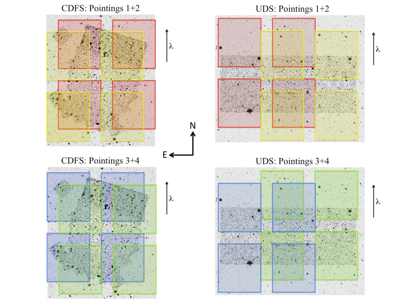
Figure 1: Layout of the eight VANDELS pointings, four in UDS and four in CDFS. In each figure the VIMOS quadrants of a given pointing are shown as a different colour, overlaid on a greyscale image showing the HST $H-$band imaging provided by the CANDELS survey (Grogin et al. 2011; Koekemoer et al. 2011) in the central regions and ground-based $H-$band imaging from the UKIDSS UDS (Almaini et al., in preparation) and VISTA VIDEO (Jarvis et al. 2013) surveys covering the wider fields. The total area covered by the eight VIMOS pointings is $\simeq 0.2$ square degrees. The spectroscopic slits are all placed E-W on the sky, as recommended to minimise slit losses during long VIMOS integrations on fields at these declinations (Sánchez-Janssen et al., 2014).

2.4 Legacy Science

Although the science cases outlined above provided the primary motivation, as an ESO public spectroscopy survey, the greatest strength of VANDELS is arguably its long-term legacy value to the astronomical community. In general terms, by providing high SNR continuum spectroscopy of galaxies which traditionally only have Ly$\alpha$ redshifts at best, VANDELS is guaranteed to open up new parameter space for investigating the physical properties of high-redshift galaxies.

More specifically, the VANDELS spectra provide the opportunity to accurately determine the fraction of Ly$\alpha$ emitters amongst the general Lyman-break galaxy population in the redshift range $3.0<z<6.0$, thereby providing an improved baseline measurement for studies within the reionization epoch (e.g. Curtis-Lake et al. 2012; Pentericci et al. 2014; De Barros et al. 2017). In addition, VANDELS will also provide large samples of spectroscopically-confirmed galaxies at $z\simeq 3$ with which to identify and study Lyman continuum emitters (e.g. Vanzella et al. 2016; de Barros et al. 2016; Shapley et al. 2016; Marchi et al. 2017). Moreover, combining the VANDELS spectra with near-IR spectroscopy offers the prospect of directly comparing stellar and gas-phase metallicities out to $z\simeq 3.5$, and constraining the possible star-formation timescales via quantifying the level of $\alpha-$enhancement (e.g. Steidel et al. 2016) as a function of stellar mass and star-formation rate. We also note that additional science will be facilitated by the samples of rarer Herschel-detected galaxies and AGN targeted by VANDELS. For these systems, the deep VANDELS spectroscopy will make it possible to assess their physical conditions (e.g. metallicities, ionizing fluxes and outflow signatures) and compare them with those of less active systems at the same redshifts.

In terms of future follow-up observations, there is an excellent synergy between VANDELS and the expected launch date of the JWST in 2020. The opportunity to combine ultra-deep optical spectroscopy with the unparalleled near-IR spectroscopic capabilities of NIRSpec will make VANDELS sources an obvious choice for follow-up spectroscopy with JWST. For high multi-plex follow-up observations, there is also an excellent overlap between the footprint of the VANDELS survey within the UDS and CDFS fields and the the field of view of ESO’s forthcoming Multi Object Optical and Near-infrared Spectrograph (MOONS) for the VLT (Cirasuolo et al., 2014).

Finally, it is also worth noting that the declinations of the UDS and CDFS fields make them ideal for sub-mm and mm follow-up observations with ALMA. One of the key scientific questions that VANDELS will help to address is the evolution of star formation and metallicity in galaxies at $z\geq 2$. However, in order to derive a complete picture it will be necessary to obtain dust mass and star-formation rate measurements at long wavelengths, which can now be provided by short, targeted, continuum observations with ALMA.

3 Field Choice

The VANDELS survey targets two fields, the UKIDSS Ultra Deep Survey (UDS: 02:17:38, $-$05:11:55) and the Chandra Deep Field South (CDFS: 03:32:30, $-$27:48:28). Both fields were selected on the basis of their observability from Paranal and the quality of their existing multi-wavelength ancillary data. We note that the COSMOS field, which was also actively considered for inclusion in VANDELS, was targeted with VIMOS by the ESO public spectroscopy survey LEGA-C (van der Wel et al., 2016).

Both the UDS and CDFS offer deep optical-nearIR HST imaging provided by the CANDELS survey (Grogin et al. 2011; Koekemoer et al. 2011) with the CDFS also offering deep HST/ACS optical imaging from the original GOODS survey (Giavalisco et al., 2004) and ultra-deep X-ray imaging (Luo et al., 2017). Moreover, both fields feature the deepest available Spitzer IRAC imaging on these angular scales from the S-CANDELS survey (Ashby et al., 2015) and deep WFC3/IR grism spectroscopy from the public 3D-HST programme (Brammer et al., 2012). When combined with the deepest available $Y+K$ imaging from the HUGS survey (Fontana et al., 2014), it is clear that the UDS and CDFS are excellent legacy fields for studying the high-redshift Universe.

Given that a single pointing of the VIMOS spectrograph covers an area larger than the HST imaging in any of the five CANDELS fields, another important consideration when choosing which fields to target with VANDELS was the quality of the ancillary data over a wider area. The importance of the wider-field ancillary data can be seen from Fig. 1, which shows the layout of the eight VIMOS pointings targeted by the VANDELS survey in UDS and CDFS. It can be seen that, although the VIMOS pointings are arranged to ensure that all of the deep WFC3/IR imaging is covered, approximately 50% of the full VANDELS survey footprint lies outside the central areas of the UDS and CDFS fields that are covered by HST imaging. Crucially, in both the UDS and CDFS, these wider-field regions are covered by high-quality, publicly-available, optical-nearIR imaging data from a wide variety of different ground-based telescopes (see Table 1).

Table 1: Details of the imaging data included in the new photometric catalogues generated for the wide-field areas of the CDFS and UDS fields. Column 1 lists the field, column 2 lists the filters, column three lists the median 5$\sigma$ depths measured within a $2^{\prime\prime}-$diameter aperture, column 4 lists the telescopes on which the imaging was obtained and column 5 lists the paper where the data are presented. For the two filters tagged with a $\dagger$ in column 2, the $5\sigma$ depth refers to the depth measured after the HST imaging was convolved to match the 1.0^′′ FWHM spatial resolution of the ground-based imaging in CDFS. The filters listed as ‘IA’ in column 2 are medium-band filters and NB921 is a narrow-band filter. The two $z-$band filters listed for the UDS field (z${}_{1}^{\prime}$ and z${}_{2}^{\prime}$) refer to imaging obtained with the Suprime-Cam z${}^{\prime}-$filter before and after the CCD detectors were upgraded. The references listed in column 5 correspond to: (1) Almaini et al., in preparation, (2) Furusawa et al. (2008), (3) Furusawa et al. (2016), (4) Sobral et al. (2012), (5) Jarvis et al. (2013), (6) Nonino et al. (2009), (7) Cardamone et al. (2010), (8) Rix et al. (2004), (9) Hsieh et al. (2012).

Field	Filter	Depth($5\sigma$)	Telescope	Reference
UDS	U	27.0	CFHT	1
	B	27.8	Subaru	2
	V	27.4	Subaru	2
	R	27.2	Subaru	2
	i′	27.0	Subaru	2
	z${}_{1}^{\prime}$	26.0	Subaru	2
	z${}_{2}^{\prime}$	26.4	Subaru	3
	NB921	25.8	Subaru	4
	Y	25.1	VISTA	5
	J	25.5	UKIRT	1
	H	24.9	UKIRT	1
	K	25.1	UKIRT	1
CDFS	U	27.8	VLT	6
	B	27.1	ESO 2.2m	7
	IA484	26.4	Subaru	7
	IA527	26.4	Subaru	7
	IA598	26.2	Subaru	7
	V${}_{606}\dagger$	26.6	HST	8
	IA624	26.0	Subaru	7
	IA651	26.3	Subaru	7
	R	27.2	VLT	1
	IA679	26.2	Subaru	7
	IA738	26.1	Subaru	7
	IA767	25.1	Subaru	7
	z${}_{850}\dagger$	25.6	HST	8
	Y	24.5	VISTA	5
	J	24.7	CFHT	9
	H	23.8	VISTA	5
	K	24.1	CFHT	9

4 Target selection

The ideal situation when selecting targets for a spectroscopic survey is to utilise a single photometric catalogue that provides consistent photometry with uniform wavelength coverage over the full survey area. Unfortunately, this was not possible when performing target selection for the VANDELS survey for two fundamental reasons. Firstly, given that VANDELS targeted two separate survey fields, covered by different sets of imaging data, it is clear that target selection had to be performed using a minimum of two independent photometric catalogues.

Secondly, as described above, the footprint of the VANDELS survey within the UDS and CDFS fields covers both the central areas with deep HST imaging and the wider-field areas covered primarily by ground-based imaging (see Fig. 1). As a result, the VANDELS survey area is effectively divided into four regions: UDS-HST, UDS-GROUND, CDFS-HST and CDFS-GROUND, each of which required a separate photometric catalogue. Consequently, the first stage in the target selection process was the adoption or production of robust photometric catalogues for each of the four regions.

4.1 Photometric catalogues

Within the two regions covered by the WFC3/IR imaging provided by the CANDELS survey (UDS-HST and CDFS-HST), we adopted the $H-$band selected photometric catalogues produced by the CANDELS team (Galametz et al. 2013; Guo et al. 2013). Both catalogues provide PSF-homogenised photometry for the available ACS and WFC3/IR imaging, in addition to spatial-resolution matched photometry from Spitzer IRAC and key ground-based imaging data sets derived using the tfit software package (Laidler et al., 2007). We refer the reader to Galametz et al. (2013) and Guo et al. (2013) for full details of the production of these photometric catalogues for the CANDELS UDS and CANDELS CDFS fields, respectively.

Within the wider-field areas there were no publicly available, near-IR selected, photometric catalogues which met our target selection requirements. As a result, new multi-wavelength photometric catalogues were generated using the publicly available imaging. The imaging in both the UDS and CDFS fields was initially accurately registered and placed on the same pixel scale and photometric zero-point. The imaging in the CDFS field had seeing which varied within the range $0.6-1.0^{\prime\prime}$ FWHM. As a result, it was necessary to PSF-homogenise the images to a common spatial resolution of $1.0^{\prime\prime}$ FWHM using Gaussian convolution kernels. The imaging in the UDS field had a much narrower range of seeing ($0.8\pm 0.05^{\prime\prime}$ FWHM), meaning that PSF-homogenisation was not necessary.

Following this initial processing, the photometric catalogues were generated with sextractor v2.8.6 (Bertin & Arnouts, 1996) in dual-image mode, using the $H-$band images as the detection images. Object photometry was measured within $2^{\prime\prime}-$diameter circular apertures, with accurate errors calculated on an object-by-object basis using the aperture-to-aperture variance between local blank-sky apertures (see Mortlock et al. 2017 for full details).

In Table 1 we provide details of the imaging data incorporated within the new photometric catalogues for the UDS-GROUND and CDFS-GROUND regions. All of the depths listed in Table 1 refer to the data that were publicly available and included in the target selection catalogues in summer 2015. We note that, since that date, many of the near-IR data sets have increased in depth significantly, particularly within the extended CDFS field. Therefore, to accompany the final data release of the VANDELS survey, we are committed to publicly releasing updated photometric catalogues, including deeper data where available, along with photometric redshifts and stellar-population parameters derived via SED fitting.

4.2 Photometric redshifts

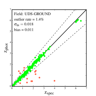
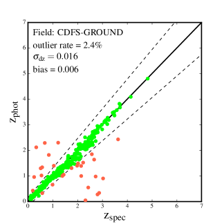
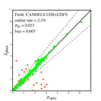
Figure 2: Top: photometric redshifts derived by the VANDELS team compared to robust spectroscopic redshifts in the wide-area region of the UDS (red data-points are catastrophic outliers with $|{\rm dz}|>0.15$). Middle: equivalent plot for the wide-area region of the CDFS. Bottom: photometric redshift versus spectroscopic redshift for those objects in the top two panels for which photometric redshifts derived by the CANDELS survey team were available (see text for more details). The catastrophic outlier fraction, $\sigma_{\rm dz}$ and bias are displayed in the top-left corner of each panel.

A key element of the VANDELS survey strategy was the use of robust photometric-redshift pre-selection. For this process to be successful it was of paramount importance to either adopt or derive photometric redshifts of equal quality within all four of the VANDELS regions. For the two regions covered by deep HST near-IR imaging (UDS-HST and CDFS-HST), we adopted the photometric redshifts made publicly available by the CANDELS survey team (Santini et al., 2015). As discussed in Dahlen et al. (2013), these photometric redshifts are derived by optimally combining the independent estimates produced by a variety of different photometric-redshift codes.

For the wider-area regions outside of the CANDELS WFC3/IR imaging footprint, new photometric redshifts were generated within the VANDELS team, based on the new UDS-GROUND and CDFS-GROUND photometric catalogues. These photometric redshifts were derived by taking the median value of $z_{\rm phot}$ for each galaxy, based on a total of fourteen different photometric redshift estimates derived by different members of the VANDELS team. The fourteen different photometric redshift estimates were produced using a variety of different publicly-available codes (e.g. Arnouts et al. 1999; Bolzonella et al. 2000; Ilbert et al. 2006; Brammer et al. 2008; Feldmann et al. 2006) and in-house software (e.g. Fontana et al. 2000; McLure et al. 2011), using a wide variety of different SED templates, star-formation histories, metallicities and emission-line prescriptions.

In order to optimise their respective photometric-redshift codes, each member of the VANDELS team taking part in the photometric-redshift exercise was initially allocated a spectroscopic training set for the UDS-GROUND and CDFS-GROUND regions. Each training set consisted of approximately one thousand high-quality spectroscopic redshifts, and were used by each team member to optimise the performance of their code. The second step in the process was to allocate spectroscopic validation sets to each member of the photometric-redshift team. The spectroscopic validation sets were identical in size and quality to the corresponding training sets, the only difference being that the spectroscopic redshifts were not disclosed to the team members. The accuracy of the results on these blind validation sets was used to ensure that each set of photometric-redshift estimates was adding useful information to the overall result. For the UDS-GROUND region the robust spectroscopic redshifts used for training and validation purposes were drawn from the VIPERS survey (Guzzo et al., 2014a), the 3D-HST survey (Momcheva et al., 2016) and the UDSz survey (Almaini et al., in preparation). For the CDFS-GROUND region the robust spectroscopic redshifts were drawn from the large number of spectroscopic redshift campaigns previously undertaken within the field (e.g. Le Fèvre et al. 2005; Mignoli et al. 2005; Vanzella et al. 2008; Balestra et al. 2010; Cooper et al. 2012; Le Fèvre et al. 2013; Momcheva et al. 2016).

To quantify the quality of the photometric redshift estimates we calculate three statistics. To quantify any systematic off-set between the photometric and spectroscopic redshifts we calculate the bias, which we define as the median value of $dz~{}=~{}(z_{\rm spec}~{}-~{}z_{\rm phot})~{}/~{}(~{}1~{}+~{}z_{\rm spec})$. Secondly, to quantify the accuracy of the photometric redshifts, we calculate $\sigma_{\rm dz}$ using the robust median absolute deviation (MAD) estimator. Finally, we also calculate the fraction of catastrophic outliers, where an object is considered to be a catastrophic outlier if $|dz|>0.15$. Based on the spectroscopic validation sets, the fourteen individual photometric-redshift runs produced bias values in the range $0.03-0.003$, values of $\sigma_{\rm dz}$ in the range $0.018-0.058$ and catastrophic outlier rates between 2% and 16%. The equivalent statistics for the adopted median combined $z_{\rm phot}$ results are bias= 0.008, $\sigma_{\rm dz}=0.017$ and a catastrophic outlier rate of 1.9%. Compared to the best-performing individual photometric redshift run, the process of median combination has produced a $15\%$ improvement in both $\sigma_{\rm dz}$ and the catastrophic outlier fraction, with the same level of bias. In Fig. 2 we show the accuracy of the final photometric redshifts adopted for the wider-area UDS-GROUND and CDFS-GROUND regions, based on the spectroscopic validation sets.

Within the final spectroscopic validation sets used to define the accuracy of the VANDELS photometric redshifts, 44% of the galaxies also had photometric redshifts determined by the CANDELS team. As a result, it was possible to perform a useful comparison of the quality of our new photometric redshifts, based on the photometric data listed in Table 1, and the photometric redshifts derived by the CANDELS survey team based on a combination of deep HST imaging, ground-based imaging and Spitzer IRAC imaging. For the objects in common, the VANDELS photometric redshifts have a catastrophic outlier rate of 2.0% and $\sigma_{\rm dz}=0.018$, virtually identical to the statistics for the full validation sets. The equivalent statistics for the CANDELS photometric redshifts are an outlier rate of 2.2% and $\sigma_{\rm dz}=0.023$ (see bottom panel of Fig. 2). The results of this comparison suggest that the VANDELS photometric redshifts are slightly more accurate that the photometric redshifts derived by the CANDELS survey team.

In summary, we are confident that by combining the results of the CANDELS and VANDELS teams we were able to produce a final set of photometric redshifts of consistent quality over all four of the VANDELS regions, irrespective of the availability of deep HST imaging data.

4.3 Star-galaxy separation

In order to produce the cleanest selection catalogue possible, it was necessary to remove potential stellar sources. Due to the high angular resolution provided by HST, this was a straightforward process for the photometric catalogues within the UDS-HST and CDFS-HST regions. All sources originating from the Galametz et al. (2013) and Guo et al. (2013) catalogues were excluded if they had a sextractor (Bertin & Arnouts, 1996) stellaricity parameter of CLASS$\_$STAR $\geq 0.98$. Following the application of this criteria to remove stellar sources, it was confirmed that the UDS-HST and CDFS-HST photometric catalogues no longer displayed a stellar locus in a variety of different colour-colour diagrams.

For the two ground-based photometric catalogues, all sources consistent with the stellar locus on the $BzK$ diagram (Daddi et al., 2004) were excluded. In addition, all remaining sources had their SED fitted with a range of stellar templates drawn from the SpeX archive. All sources which produced an improved SED fit with a stellar template and were consistent with being a point source at ground-based resolution were excluded. It should be noted that $<5\%$ of the objects in the two ground-based photometric catalogues were excluded as being potentially stellar. Morevoer, it is noteworthy that $98\%$ of the excluded objects had $z_{\rm phot}<1$ and would therefore not even have entered the VANDELS parent sample (see Section 4.5).

4.4 Physical properties and rest-frame photometry

At this stage, a final run of SED fitting was carried out in order to derive star-formation rates, stellar masses and rest-frame photometry. This SED fitting was performed using Bruzual & Charlot (2003) templates with solar metallicity and no nebular emission. Exponentially-declining star-formation histories were employed, with $\tau$ in the range $0.3\leq\tau\leq 20$ Gyr, and ages were constrained to lie between 50 Myr and the age of the Universe at the redshift of interest. Dust attenuation was described using the Calzetti et al. (2000) starburst attenuation law, with $A_{\rm V}$ in the range $0.0\leq A_{\rm V}\leq 2.5$, and IGM absorption was accounted for using the Madau (1995) prescription. These parameters were adopted following the results of Wuyts et al. (2011), who showed that this parameter set does a reasonable job of recovering the total star-formation rate of main-sequence galaxies, provided that they are not heavily obscured. We also note that this SED parameter set is very similar to that adopted by the 3D-HST survey team (Momcheva et al., 2016) and delivers stellar-mass estimates in good agreement with those derived for the CANDELS CDFS and UDS photometric catalogues by Santini et al. (2015). During the SED-fitting process the redshift was fixed at the median value derived from the multiple photometric-redshift runs described in Section 4.2.

Further cleaning of the sample was carried out based on the results of the SED fitting. For each of the four photometric catalogues, plots of the SED fits for the objects comprising the worst 10% of fits (i.e. highest $\chi^{2}$), were visually examined. Objects that were revealed by this process to have unreliable or discrepant photometry were excluded from the sample ($\simeq 4\%$ of objects).

4.5 Parent spectroscopic sample

Armed with catalogues providing robust photometry, photometric redshifts and physical properties, it was then possible to select the parent sample of potential spectroscopic targets. The vast majority (i.e. $\simeq 97$%) of the potential targets were drawn from three main target categories:

• Bright star-forming galaxies in the range $2.4\leq z\leq 5.5$

• Lyman-break galaxies in the range $3.0\leq z\leq 7.0$

• Passive galaxies in the range $1.0\leq z\leq 2.5$

while the remaining $\simeq 3$% of potential targets were either known or candidate AGN ($\simeq 2$%), or Herschel-detected galaxies ($\simeq 1$%).

4.5.1 Bright star-forming galaxies

This sub-sample consists of bright star-forming galaxies within the redshift range $2.4\leq z\leq 5.5$ with $i\leq 25$. The redshift range is designed to ensure that the UV absorption features necessary for investigating stellar metallicity lie within the $0.48<\lambda<1.0$ $\mu$m wavelength coverage of the VANDELS spectra. The magnitude constraint is designed to ensure that the final VANDELS spectra have sufficient SNR to allow absorption-line studies on individual objects. In order to be classified as actively star-forming, each member of this sub-sample was required to satisfy: sSFR > 0.1 Gyr^-1, where sSFR is the specific star-formation rate (SFR/$M_{\ast}$) derived from the SED fitting described in Section 4.4. In reality, 99% of this sub-sample satisfy the criteria: sSFR > 0.6 Gyr^-1, ensuring that they are fully consistent with being located on the main sequence of star formation (see Fig. 3).

4.5.2 Lyman-break galaxies

This sub-sample consists of fainter star-forming galaxies within the redshift range $3.0\leq z\leq 7.0$. The vast majority (95%) of the galaxies in this sub-sample lie in the redshift interval $3.0~{}\leq~{}z\leq~{}5.5$ and in the HST regions have $25\leq H\leq 27\land i\leq 27.5$. In the wider-field regions these objects have $i\leq 26.0$. The remainder of the sub-sample consists of galaxies selected to have redshifts in the range $5.5~{}\leq~{}z~{}\leq~{}7.0$ and, in the HST regions, to have $25\leq H\leq 27$ and $z^{\prime}\leq 26.5$ (UDS-HST) or $z_{850}\leq 27.0$ (CDFS-HST). In the wider-field regions these objects have $z^{\prime}\leq 26.0$ and $z_{850}\leq 25.0$ in the UDS-GROUND and CDFS-GROUND regions, respectively. The change in selection criteria for the $z\geq 5.5$ targets was mandatory, due to the impact of IGM absorption on $i-$band photometry at these redshifts. Once again, the formal requirement for these galaxies to be classified as star-forming was that sSFR > 0.1 Gyr^-1. However, in reality, 99% of the galaxies in this sub-sample have sSFR > 0.3 Gyr^-1 and provide a good sampling of the main sequence of star formation (see Fig. 3).

4.5.3 Passive galaxies

This sub-sample consists of $UVJ-$selected (Williams et al. 2009; Whitaker et al. 2011) passive galaxies in the redshift interval $1.0\leq z\leq 2.5$ with $H\leq 22.5\land i\leq 25$. The $H-$band magnitude constraint for this sub-sample is designed to impose an effective lower stellar-mass limit of $\log(M_{\ast}/\hbox{$\rm\thinspace M_{\odot}$})\geq 10$. As with the bright star-forming galaxy sub-sample, the $i-$band magnitude constraint is designed to ensure that the final individual spectra are deep enough to allow detailed absorption-line studies. The $UVJ$ selection was performed using the rest-frame photometry derived from the SED fitting described in Section 4.4. Galaxies which satisfied all of the following criteria were identified as passive:

$$\begin{split}U-V&>0.88(V-J)+0.49,\\ U-V&>1.2,\\ V-J&<1.6.\end{split}$$ (1)

We note here that although these galaxies are classified as passive, it is not the case that they are necessarily expected to exhibit no on-going star-formation. Based on the results of the SED fitting, 94% of the $UVJ-$selected passive galaxies do have estimated values of sSFR<0.1 Gyr^-1, clearly separating them from main-sequence galaxies. However, $3\%$ of the $UVJ-$selected passive galaxies have sSFR > 0.3 Gyr^-1, placing them in a location on the SFR$-M_{\ast}$ diagram consistent with the low-SFR tail of the main sequence. This is not unexpected, given that $UVJ$ selection is inevitably vulnerable to contamination by dusty star-forming galaxies at some level.

4.5.4 AGN and Herschel-detected galaxies

The candidate AGN all lie within the CDFS field and were selected based on either a power-law SED shape in the mid-IR (Chang et al., 2017) or X-ray emission (Xue et al. 2011; Rangel et al. 2013; Hsu et al. 2014). Within the CDFS-HST region the candidate AGN were restricted to $z\geq 2.4$ and $i\leq 27.5$, while in the CDFS-GROUND region they were restricted to $z\geq 2.4$ and $i\leq 26$. The Herschel-detected galaxies all lie within the UDS-HST and CDFS-HST regions, have $z\geq 2.4$ and $i\leq 27.5$, and are detected in at least one Herschel band (c.f. Pannella et al. 2015). We note here that the photometric redshifts derived for the AGN candidates are based on SED fitting with the same set of galaxy templates discussed in Section 4.2, and are therefore not expected to be as accurate as the photometric redshifts derived for the rest of the VANDELS sample.

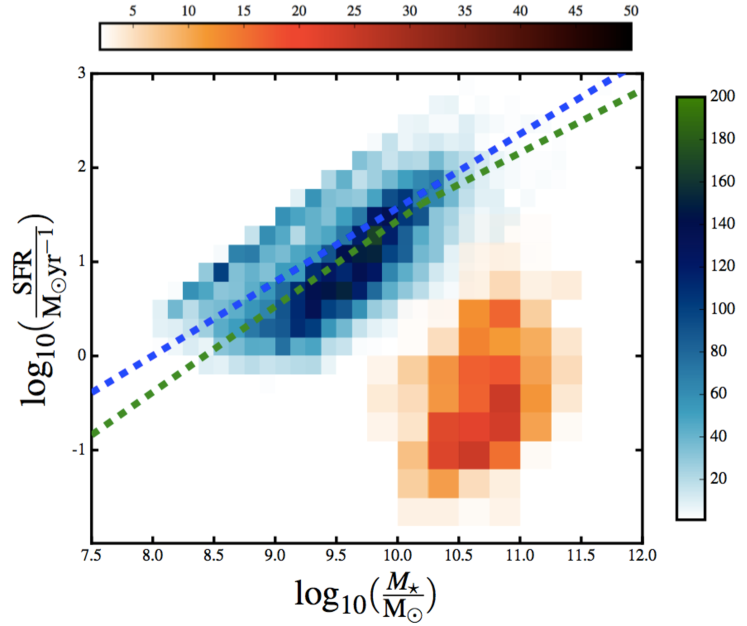
Figure 3: The distribution of the VANDELS parent sample on the SFR$-M_{\ast}$ plane. The blue-shaded 2D histogram shows the location of the star-forming galaxies (including additional candidate AGN and Herschel sources) in the redshift interval $2.4\leq z\leq 7.0$ (median redshift $z=3.4$). The red-shaded histogram shows the location of the passive galaxy sub-sample in the redshift interval $1.0\leq z\leq 2.5$ (median redshift $z=1.2$). The horizontal and vertical colour bars indicate the number of galaxies within each 2D bin. The blue and green dashed lines show determinations of the main sequence of star-formation at $z=3$ and $z=2.5$ by Speagle et al. (2014) and Whitaker et al. (2014), respectively. It can be seen that the VANDELS galaxies successfully sample the main sequence of star-formation and the area of parameter space occupied by massive, quenched galaxies. In total, the VANDELS spectroscopic sample spans 3.5 dex in stellar mass and 4.5 dex in star-formation rate.

4.5.5 Summary

Following the application of the selection criteria outlined above, a final visual check was performed on the entire sample to ensure that no image artefacts had survived the selection procedure. The resulting parent sample of potential VANDELS spectroscopic targets consisted of 9656 galaxies, split roughly equally between the UDS and CDFS fields. The distribution of the parent sample on the SFR$-M_{\ast}$ plane is shown in Fig. 3, from which it can be seen that the adopted selection criteria successfully isolated the main sequence of star formation and the high stellar-mass quenched population. Overall, the parent VANDELS sample spans 3.5 dex in stellar mass and 4.5 dex in star-formation rate.

4.6 Final spectroscopic sample

Table 2: The distribution of the 2106 spectroscopic slits targeted within the VANDELS survey between the two survey fields, the different target classifications and the different integration times. The first column lists the survey field. Column two lists the number of slits allocated to bright star-forming galaxies (SFG), column three lists the number of slits allocated to massive, passive galaxies (PASS), column four lists the number of slits allocated to fainter star-forming galaxies (LBG) and the fifth column lists the number of slits allocated to AGN candidates or Herschel-detected galaxies (AH). Note that all of the AGN candidates were selected in the CDFS field due to the availability of ultra-deep X-ray data (Luo et al., 2017).The final three columns list the number of slits allocated to objects which require 20, 40 and 80 hours of on-source integration, respectively.

FIELD	SFG	PASS	LBG	AH	20	40	80
UDS	224	151	693	10	303	550	225
CDFS	200	117	656	55	238	528	262
TOTAL	424	268	1349	65	541	1078	487

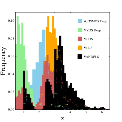
Figure 4: A comparison of the redshift distributions of large-scale spectroscopic surveys carried out with the VIMOS spectrograph. The deep component of the zCOSMOS survey (Lilly et al., 2007) is shown in blue and the deep component of the VIMOS VLT Deep Survey (VVDS) is shown in green (Le Fèvre et al., 2013). The VIMOS Ultra Deep Survey (VUDS) is shown in red (Le Fèvre et al., 2015) and the VLT LBG Redshift Survey (VLRS) is shown in orange (Bielby et al., 2013). The black histogram shows the photometric redshift distribution of the final sample of 2106 galaxies targeted by the VANDELS survey.

Using the parent sample as input, extensive simulation work was undertaken in order to maximise the number of slits which could be allocated across the eight VIMOS pointings. In addition to the total number of spectroscopic slits, the primary goal of this experimentation was to maximise the number of slits allocated to bright star-forming galaxies and massive passive galaxies, the two classes of targets with the lowest surface densities. Apart from the photometric redshift and magnitude constraints outlined above, the only additional constraint applied to the simulations was the desire to allocate the slits to objects requiring 20, 40 and 80 hours of integration in an approximately 1:2:1 ratio. Crucially, during the slit allocation process, no additional prioritisation was applied based on source brightness, redshift or position.

The overall result of the target selection process was a final sample of 2106 galaxies being allocated to spectroscopic slits. The distribution of the spectroscopic slits between the two survey fields, the different target classifications and the different amounts of required exposure time are detailed in Table 2. The final spectroscopic samples of bright star-forming galaxies and passive galaxies are random (approximately 1 in 4) sub-samples drawn from the corresponding targets within the input parent spectroscopic sample. Likewise, the final spectroscopic sample of Lyman-break galaxies is a random (approximately 1 in 5) sub-sample of the Lyman-break targets within the parent spectroscopic sample. In Fig. 4 we compare the photometric-redshift distribution of the final VANDELS sample to the spectroscopic redshift distributions of comparable large-scale spectroscopic surveys previously carried out using the VIMOS spectrograph.

5 Observing strategy

As illustrated in Fig. 1, the VANDELS survey consists of a total of eight VIMOS pointings, four overlapping pointings in UDS and four overlapping pointings in CDFS. In both fields the pointing centres were chosen to provide both contiguous coverage and to fully sample the central areas with deep HST imaging. Fully covering the deep HST imaging was essential in order to allow access to a high surface-density of faint $z\geq 3$ targets.

5.1 Signal-to-noise requirements

The VANDELS observing strategy was designed to provide consistently high SNR continuum detections for the bright star-forming and passive galaxy sub-samples. For those objects with $i\leq 24.5$, the final 1D spectra are designed to have a SNR in the range $15-20$ per resolution element, within the wavelength range $6000<\lambda<7400$ Å, based on 20 or 40 hours of on-source integration (where one resolution element is 4 pixels, or 10.2Å). For the faintest objects in these sub-samples ($i\simeq 25$), the final spectra are designed to have SNR $\simeq 10$, based on 80 hours of integration. For the fainter ($H\leq 27\land i\leq 27.5$) Lyman-break galaxies at $z\geq 3$, the VANDELS observing strategy is designed to provide SNR $\geq 3$ in the continuum, and a consistent Ly$\alpha$ emission-line detection limit of $\simeq 2\times 10^{-18}$ erg s^-1cm^-2 ($5\sigma$, integrated over a line profile with FWHM=10Å).

In order to achieve the desired SNR, targets were allocated 20, 40 or 80 hours of on-source integration according to two different exposure time schemes. The bright star-forming and passive galaxies were allocated 20 hours of integration time if $i_{2}\leq 23.75$, 40 hours in the range $23.75<i_{2}\leq 24.25$ and 80 hours in the range $24.25<i_{2}\leq 25.00$ (where $i_{2}$ is the $i-$band magnitude measured in a 2${}^{\prime\prime}-$diameter circular aperture at ground-based resolution). The LBGs, AGN candidates and Herschel-detected galaxies were allocated 20, 40 or 80 hours of integration time within the following three magnitude ranges: $25.00<i_{2}\leq 25.50$, $25.50<i_{2}\leq 26.00$ and $26.00<i_{2}\leq 27.50$. The highest-redshift LBG targets at $z\geq 5.5$ followed the same exposure time scheme as the main LBG sub-sample, except with the $i-$band magnitudes replaced with $z-$band magnitudes.

5.2 Nested slit allocation policy

To accommodate the required range of exposure times, the VANDELS survey employed a nested slit allocation strategy. Each of the eight VIMOS pointings was observed using four sets of masks, with each set receiving 20 hours of on-source integration time. Consequently, objects which required 80 hours of integration were retained on all four masks, those requiring 40 hours were included on two masks and those requiring 20 hours only appeared on a single mask. As can be seen from Table 2, approximately 75% of the galaxies targeted by the VANDELS survey received 40+ hours of on-source integration.

5.3 Observations

All of the VANDELS observations used the MR grism+GG475 order sorting filter, 1 arcsec slit widths and a minimum slit length of 7 arcsec. This set-up provides wavelength coverage of 480$-$1000 nm, with a dispersion of 0.255 nm/pix and a mean spectral resolution of $R\simeq 580$. All of the slits were oriented E-W on the sky, as recommended for minimising slit losses when pursuing long integrations of the UDS and CDFS fields from Paranal (Sánchez-Janssen et al., 2014). To ensure that the VIMOS slits were placed with maximum accuracy, short $R-$band pre-images were obtained in service mode during P94, in order to properly account for VIMOS focal plane distortions and allocate 1–2 bright reference stars to each VIMOS mask.

All observations were obtained using observing blocks (OBs) designed to deliver a total of one hour of on-source integration time. Each OB consisted of three integrations of 1200s, obtained in a three-point dither pattern, with off-sets of 0, $-$4 pixels, +8 pixels, corresponding to 0.0, $-0.82$ and +1.64 arcsec respectively. One arc frame and one flat-field frame were obtained for calibration purposes after the execution of two consecutive OBs. A spectrophotometric standard was observed at least once every seven nights and at least once per observing run. Further details of the VANDELS observations can be found in the data release paper (Pentericci et al., 2018).

6 Data Reduction and Spectroscopic Redshift Measurement

The reduction of the VANDELS data set is performed with the fully-automated easylife pipeline, starting from the raw data and ending with the fully wavelength- and flux-calibrated one-dimensional spectra. The easylife pipeline (Garilli et al., 2012) is an updated version of the original vipgi system (Scodeggio et al., 2005). The original vipgi system was used to reduce all the spectra from the VVDS (Le Fèvre et al. 2005; Garilli et al. 2008), zCosmos (Lilly et al., 2007) and VUDS surveys (Le Fèvre et al., 2015), while the updated system easylife was used to reduce all of the spectra from the recently completed VIPERS survey (Guzzo et al., 2014b). A detailed description of the full data reduction process can be found in Pentericci et al. (2018).

In addition to the reduced spectra, it is a requirement of the ESO public survey agreement for VANDELS that the team provide spectroscopic redshift measurements for each of the spectra released via the ESO data archive. The spectroscopic redshift measurements were made by a dedicated group of VANDELS team members using the ez software package (Garilli et al., 2010). The core algorithm of ez is cross-correlation using galaxy templates that, for VANDELS spectra, were predominantly derived from previous VIMOS surveys. The redshift for each galaxy was independently measured by two team members, who were subsequently required to reach agreement on the spectroscopic redshift measurement and the associated quality flag. As a final check, the spectroscopic redshifts and associated quality flags for all spectra released in DR1 were independently checked by the two Co-PIs.

The quality of the spectroscopic redshift measurements was quantified using the system originally employed by the VVDS team (Le Fèvre et al. 2005), in which every galaxy is allocated a quality flag of 0, 1, 2, 3, 4 or 9. Galaxies for which it was not possible to measure a spectroscopic redshift are allocated flag=0, while galaxies with spectroscopic redshift measurements that are believed to be 50% or 75% reliable are allocated flag=1 and flag=2, respectively. The galaxies with the most secure redshifts, based on multiple absorption/emission features, are allocated flag=3 or 4, depending on whether their redshift measurements are believed to be 95% or 100% reliable. Galaxies which have redshift measurements based on a single emission line, in most cases Ly$\alpha$, are allocated flag=9.

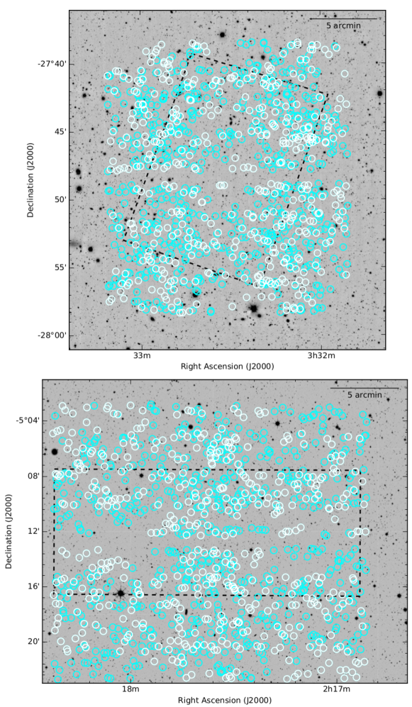
Figure 5: Finding charts showing the location of the VANDELS spectroscopic targets within the CDFS (top) and UDS (bottom) fields. The 415 targets in the CDFS and 464 targets in the UDS with spectra released in VANDELS DR1 are shown in white, with the remaining targets shown in blue. The black dashed rectangles show the approximate location of the CANDELS near-IR HST imaging (Grogin et al. 2011; Koekemoer et al. 2011). The background images are ground-based $H-$band data from the VISTA VIDEO (Jarvis et al. 2013) and UKIDSS UDS (Almaini et al., in preparation) surveys.

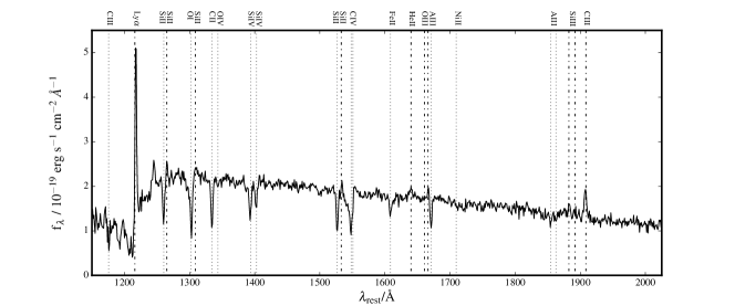
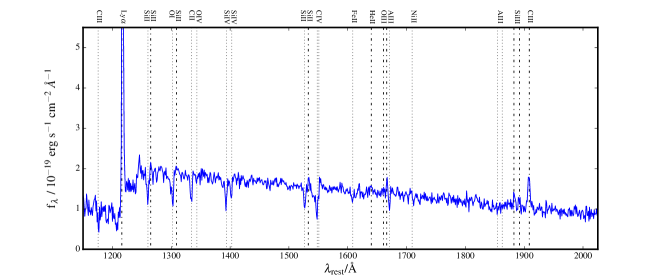
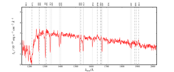
Figure 6: Median-stacked spectra of Lyman-break galaxies from VANDELS DR1. The top panel shows a stack of 105 LBGs from DR1 with robust redshifts in the range $3.0\leq z\leq 4.0$ (median redshift $z=3.5$). The middle panel shows a stack of the 61/105 galaxies that display Ly$\alpha$ in emission. The bottom panel shows a stack of the 44/105 galaxies that display Ly$\alpha$ in absorption. In all three panels, common absorption (dotted lines) and emission (dot-dashed lines) features are highlighted.

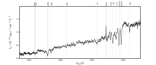
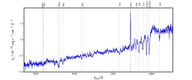
Figure 7: Median-stacked spectra of passive galaxies from VANDELS DR1. The top panel shows a stack of 65 passive galaxies from DR1 with robust redshifts in the range $1.0\leq z\leq 2.5$ (median redshift $z=1.2$). The middle panel shows a stack of the 33/65 passive galaxies that display [Oii] emission. The bottom panel shows a stack of the 32/65 passive galaxies without [Oii] emission. Common absorption (dotted lines) and emission (dot-dashed lines) features are highlighted in each panel.

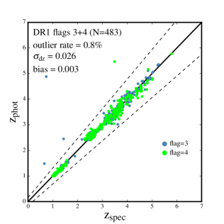
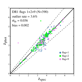
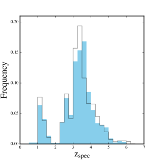
Figure 8: The top panel shows a comparison between the input photometric redshifts and measured spectroscopic redshifts for DR1 galaxies with redshift quality flags 3 and 4. The middle panel is the equivalent plot for DR1 galaxies with redshift quality flags 1, 2 and 9. Those galaxies falling outside the dashed lines are catastrophic outliers with $|{\rm dz}|>0.15$. In both panels, candidate AGN and Herschel-detected galaxies are plotted as open symbols. The bottom panel shows a comparison of the spectroscopic redshift distribution of the DR1 galaxies (solid blue histogram) and the photometric redshift distribution of the full VANDELS parent sample (open histogram).

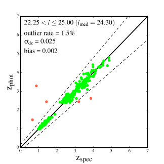
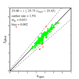
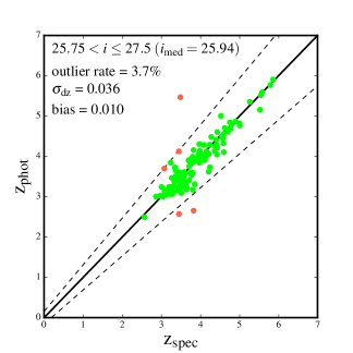
Figure 9: The top panel shows a comparison between the input photometric redshifts and measured spectroscopic redshifts for DR1 galaxies in the magnitude range $22.25<i\leq 25.00$. The middle and bottom panels show the equivalent plots for DR1 galaxies in the magnitude ranges $25.00<i\leq 25.75$ and $25.75<i\leq 27.50$, respectively. All three panels include all DR1 galaxies with spectroscopic redshift quality flags in the range $1-9$.

7 Data Release One

The first public data release for the VANDELS survey (DR1) was made by the ESO Science Archive Facility (archive.eso.org) on 29th September 2017, and features spectra obtained during the first VANDELS observing season from August 2015 until February 2016; ESO run numbers 194.A-2003(E-K). The data release includes fully flux- and wavelength-calibrated 1D spectra, plus wavelength calibrated 2D spectra, for all the VANDELS targets that received their total scheduled integration time during season one. In addition, the data release also includes spectra for those targets that had received 50% of their scheduled integration time by the end of season one.

In total, DR1 contains spectra for 879 galaxies, 415 from the CDFS pointings and 464 from the UDS pointings. In Fig. 5 we show finding charts for the CDFS and UDS fields which show the locations of the full VANDELS target list in blue, with the locations of those VANDELS targets featured in DR1 in white. In addition to the reduced spectra, DR1 also features an associated catalogue which provides coordinates, optical+nearIR photometry, photometric redshifts, spectroscopic redshifts and spectroscopic redshift quality flags for each target. In Figs. 6 & 7, we show examples that illustrate the potential for using the DR1 data set to produce high SNR stacked spectra.

8 Target Selection Accuracy

Based on the extensive testing described in Section 4.2, it was determined that the typical accuracy of the photometric redshifts adopted in the VANDELS target selection was $\sigma_{\rm dz}\simeq 0.02$, with a catastrophic outlier rate of $\leq 2\%$. However, as is often the case, the samples of galaxies used to validate the photometric redshifts have $i-$band magnitudes that are significantly brighter than those of the real VANDELS targets. Indeed, the median $i-$band magnitude of the galaxies used to validate the photometric redshifts is two magnitudes brighter than the median $i-$band magnitude of the DR1 galaxies. Consequently, it is clearly of interest to use the DR1 galaxies to review the accuracy of the selection process based on real, on-sky, data.

In the top panel of Fig. 8 we show a plot of $z_{\rm phot}$ versus $z_{\rm spec}$ for the galaxies released in DR1 with spectroscopic redshift quality flags 3 and 4, which together comprise 55% of the full DR1 sample. For these galaxies $\sigma_{\rm dz}=0.026$ with a catastrophic outlier rate of only 0.8%. The middle panel in Fig. 8 is the equivalent plot for those DR1 galaxies with spectroscopic redshift quality flags 1, 2 and 9, which have $\sigma_{\rm dz}=0.036$ and a catastrophic outlier rate of 3.6%. Taken together, the full DR1 sample (i.e. flags $1-9$) has an accuracy of $\sigma_{\rm dz}=0.029$ with a catastrophic outlier rate of $2.1\%$.

It is worth noting that the fraction of catastrophic outliers is actually significantly biased by the inclusion of a relatively small number of AGN candidates and Herschel-detected galaxies. If the statistics are restricted to the 97% of objects drawn from the three principal classifications of VANDELS targets (see Section 4.5), the accuracy is $\sigma_{\rm dz}=0.028$ and the catastrophic outlier rate is a remarkably low 1.2% (flags $1-9$). Given the relative faintness of the VANDELS targets, these figures provide a clear validation of the accuracy and robustness of the target selection procedure described in Section 4. Moreover, the low number of catastrophic outliers amongst those objects allocated spectroscopic quality flags 1 and 2 suggests that the VANDELS quality flags are somewhat conservative. In reality, for many of the flag 1 and 2 objects we can be very confident that the spectroscopic redshift lies within a relatively narrow range, but the spectral features simply do not allow competing redshift solutions to be reliably differentiated.

In the bottom panel of Fig. 8 the redshift distribution of the galaxies released in DR1 is shown as the filled blue histogram, based on their measured spectroscopic redshifts. The histogram indicated by the thin grey line shows the redshift distribution of the VANDELS parent sample, based on the input photometric redshifts. A comparison of the two clearly indicates that the spectroscopic redshift distribution of the real VANDELS spectra is in very close agreement to the distribution predicted by the photometric-redshift selection procedure.

The galaxies targeted by the VANDELS survey are fainter than those typically targeted by previous large spectroscopic surveys of high-redshift galaxies. Consequently, it is clearly of interest to explore how the accuracy of the VANDELS photometric redshifts varies as a function of target magnitude.

All but three of the VANDELS galaxies released in DR1 have $i-$band magnitudes in the range $22.25\leq i\leq 27.50$. Consequently, Fig. 9 shows a comparison between spectroscopic and photometric redshifts in three $i-$band magnitude ranges: $22.25<i\leq 25.00$, $25.00<i\leq 25.75$ and $25.75<i\leq 27.50$, and includes all objects with spectroscopic redshift quality flags $1-9$. The middle panel of Fig. 9 is representative of the $i-$band magnitude of the typical VANDELS source, whereas the top and bottom panels illustrate the photometric redshift accuracy at the bright and faint ends of the target magnitude distribution, respectively. The relevant statistics quantifying the quality of the agreement between the spectroscopic and photometric redshifts are displayed in the top-left corner of each panel of Fig. 9.

It is clear from Fig. 9 that in terms of bias and catastrophic outlier rate, the VANDELS photometric redshifts perform very well within the two brighter magnitude bins. Over the full magnitude range there is a gradual decrease in the photometric redshift accuracy, with $\sigma_{\rm dz}$ dropping from 0.025 to 0.036. However, given the factor of $\simeq 5$ drop in brightness between the top and bottom panels, the decrease in accuracy is not particularly dramatic. In contrast, it is clear from the bottom panel of Fig. 9 that the photometric redshifts for the faintest VANDELS targets with $i>25.75$ ($\simeq 15\%$ of the DR1 objects) do show a notable increase in both the fraction of catastrophic outliers and the bias.

Overall, the quality of the VANDELS photometric redshifts is in-line with expectations based on the spectroscopic redshift validation data (see Section 4.2). For all DR1 objects with spectroscopic quality flags $1-9$, an accuracy of $\sigma_{\rm dz}=0.029$ and a catastrophic outlier rate of 2.1% compares favourably with the results from the spectroscopic validation sets ($\sigma_{\rm dz}=0.025$ and $1.9\%$ catastrophic outliers), despite the $i-$band magnitudes of the VANDELS galaxies being two magnitudes fainter than the validation objects, on average. Interestingly, compared to the DR1 data, the overall systematic bias of the photometric redshifts is only $0.003\pm 0.002$. This is actually better than the expectation from the spectroscopic validation data ($0.008\pm 0.001$), albeit only at the $\simeq 2.5\sigma$ level.

9 Summary and timeline

In this paper we have provided an overview of the VANDELS spectroscopic survey, focusing on the scientific motivation, survey design and target selection. The original motivation for the VANDELS survey was to move beyond simple redshift determination and to provide the high SNR spectra necessary to study the physical properties of the high-redshift galaxy population. The spectra released in DR1 demonstrate that the original goals of the survey are within reach, and that the VIMOS spectrograph can be used to integrate for 20–80 hours without the final SNR being dominated by systematic effects. Combined with the unparalleled ancillary data available within the CDFS and UDS survey fields, it is clear that the VANDELS survey has the potential to become a key legacy data set for studying the evolution of high-redshift galaxies for many years to come.

The observations for the VANDELS survey were fully completed in February 2018. The second ESO public data release is currently scheduled for June 2018 and will feature all of the spectra completed, or 50% completed, by the end of the second VANDELS observing season in February 2017. The third ESO public data release is scheduled for June 2019 and will consist of the entire VANDELS spectroscopic data set.

A final data release is currently scheduled for June 2020 and will formally mark the end of the project. It is currently intended that the final data release will feature a re-reduction of the entire spectroscopic data set, incorporating improvements in the data reduction process which have been implemented over the course of the survey. In addition, the VANDELS team is committed to release two final catalogues to enhance the legacy value of the survey. The first catalogue will contain physical properties for each target (i.e. stellar masses, star-formation rates, dust attenuation and rest-frame colours) based on SED fitting of the final data set. The second catalogue will provide measurements of the fluxes and equivalent widths of significant emission/absorption features identified in the VANDELS spectra, along with their corresponding uncertainties.

¹Institute for Astronomy, University of Edinburgh, Royal Observatory, Edinburgh, EH9 3HJ, UK
²INAF, Osservatorio Astronomico di Roma, Monteporzio, Italy
³Dipartimento di Fisica e Astronomia, Università di Bologna, Via Gobetti 93/2, I-40129, Bologna, Italy
⁴INAF - Osservatorio Astrofisico di Arcetri, Largo E. Fermi 5, I-50157, Firenze, Italy
⁵Laboratoire AIM-Paris-Saclay, CEA/DRF/Irfu, CNRS France
⁶MPE, Giessenbachstrasse 1, D-85748 Garching, Germany
⁷Kavli Institute for Cosmology, University of Cambridge, Madingley Road, Cambridge CB3 0HA, UK
⁸Cavendish Laboratory, University of Cambridge, 19 J. J. Thomson Avenue, Cambridge CB3 0HE, UK
⁹INAF-Osservatorio di Astrofisica e Scienza dello Spazio di Bologna, via Gobetti 93/3, I-40129, Bologna, Italy
¹⁰European Southern Observatory, Karl-Schwarzschild-Str. 2, D-85748 Garching b. Munchen, Germany
¹¹Observatoire de Genève, Université de Genève, 51 Ch. des Maillettes, 1290, Versoix, Switzerland
¹²Department of Astronomy, The University of Texas at Austin, Austin, TX 78712, USA
¹³INAF - Astronomical Observatory of Trieste, via G.B. Tiepolo 11, I-34143 Trieste, Italy
¹⁴INAF-Istituto di Astrofisica Spaziale e Fisica Cosmica Milano, via Bassini 15, 20133, Milano, Italy
¹⁵Núcleo de Astronomía, Facultad de Ingeniería, Universidad Diego Portales, Av. Ejército 441, Santiago, Chile
¹⁶Department of Physics and Astronomy, University College London, Gower Street, London WC1E 6BT, UK
¹⁷INAF-Osservatorio Astronomico di Brera, via Brera 28, 20122 Milano, Italy
¹⁸Astrophysics, The Denys Wilkinson Building, University of Oxford, Keble Road, Oxford OX1 3RH, UK
¹⁹Kapteyn Astronomical Institute, University of Groningen, Postbus 800, 9700 AV, Groningen, The Netherlands
²⁰European Southern Observatory, Avenida Alonso de Córdova 3107, Vitacura, 19001 Casilla, Santiago de Chile, Chile
²¹School of Physics and Astronomy, University of Nottingham, University Park, Nottingham NG7 2RD, UK
²²University Observatory Munich, Scheinerstrasse 1, D-81679 Munich, Germany
²³Department of Astronomy, University of Michigan, 311 West Hall, 1085 South University Ave., Ann Arbor, MI 48109-1107, USA
²⁴Instituto de Astrofísica e Ciências do Espaço, Universidade de Lisboa, OAL, Tapada da Ajuda, P-1349-018 Lisbon, Portugal
²⁵Departamento de Física, Faculdade de Ciências, Universidade de Lisboa, Edifício C8, Campo Grande, PT1749-016 Lisbon, Portugal
²⁶Instituto de Fisica y Astronomia, Facultad de Ciencias, Universidad de Valparaiso, 1111 Gran Bretana, Valparaiso, Chile
²⁷Institute d’Astrophysique de Paris, CNRS, Université Pierre et Marie Curie, 98 bis Boulevard Arago, 75014, Paris, France
²⁸National Optical Astronomy Observatory, 950 North Cherry Ave, Tucson, AZ, 85719, USA
²⁹Harvard-Smithsonian Center for Astrophysics, 60 Garden St, Cambridge MA 20138, USA
³⁰Space Telescope Science Institute, 3700 San Martin Drive, Baltimore, MD, 21218, USA
³¹Dark Cosmology Centre, Niels Bohr Institute, University of Copenhagen, Juliane Maries Vej 30, DK-2100 Copenhagen, Denmark
³²Imperial college, Kensington, London SW7 2AZ, UK
³³Astronomy Department, University of Massachusetts, Amherst, MA01003, USA
³⁴Pontificia Universidad Católica de Chile, Instituto de Astrofísica Avda. Vicuña Mackenna 4860, Santiago, Chile
³⁵Aix Marseille Université, CNRS, LAM (Laboratoire d’Astrophysique de Marseille) UMR 7326, 13388, Marseille, France
³⁶Instituto de Astrofísica de Canarias, Calle Vía Láctea s/n, E-38205 La Laguna, Tenerife, Spain
³⁷Departamento de Astrofísica, Universidad de La Laguna, E-38200 La Laguna, Tenerife, Spain
³⁸Faculty of Physics, Ludwig-Maximilians Universität, Scheinerstr. 1, 81679, Munich, Germany
³⁹Department of Physics and Astronomy, Texas A&M University, College Station, TX 77843-4242, USA
⁴⁰Excellence Cluster, Boltzmann Strasse 2, D-85748 Garching, Germany
⁴¹Department of Physics, Durham University, South Road, DH1 3LE Durham, UK
⁴²Leiden Observatory, Leiden University, 2300 RA, Leiden, The Netherlands
⁴³Steward Observatory, The University of Arizona, 933 N Cherry Ave, Tucson, AZ, 85721, USA
⁴⁴Department of Physics and Astronomy, PAB, 430 Portola Plaza, Box 951547, Los Angeles, CA 90095-1547, USA
⁴⁵School of Physics and Astronomy, University of St. Andrews, SUPA, North Haugh, KY16 9SS St. Andrews, UK

References

- Arnouts et al. (1999) Arnouts S., Cristiani S., Moscardini L., Matarrese S., Lucchin F., Fontana A., Giallongo E., 1999, MNRAS, 310, 540
- Ashby et al. (2015) Ashby M. L. N., et al., 2015, ApJS, 218, 33
- Balestra et al. (2010) Balestra I., et al., 2010, A&A, 512, A12
- Bertin & Arnouts (1996) Bertin E., Arnouts S., 1996, A&AS, 117, 393
- Bielby et al. (2013) Bielby R., et al., 2013, MNRAS, 430, 425
- Bolzonella et al. (2000) Bolzonella M., Miralles J.-M., Pelló R., 2000, A&A, 363, 476
- Bourne et al. (2017) Bourne N., et al., 2017, MNRAS, 467, 1360
- Bouwens et al. (2016) Bouwens R. J., et al., 2016, ApJ, 833, 72
- Bowler et al. (2015) Bowler R. A. A., et al., 2015, MNRAS, 452, 1817
- Bowler et al. (2018) Bowler R. A. A., Bourne N., Dunlop J. S., McLure R. M., McLeod D. J., 2018, preprint, (arXiv:1802.05720)
- Bradshaw et al. (2013) Bradshaw E. J., et al., 2013, MNRAS, 433, 194
- Brammer et al. (2008) Brammer G. B., van Dokkum P. G., Coppi P., 2008, ApJ, 686, 1503
- Brammer et al. (2012) Brammer G. B., et al., 2012, ApJS, 200, 13
- Bruce et al. (2012) Bruce V. A., et al., 2012, MNRAS, 427, 1666
- Bruzual & Charlot (2003) Bruzual G., Charlot S., 2003, MNRAS, 344, 1000
- Calzetti et al. (2000) Calzetti D., Armus L., Bohlin R. C., Kinney A. L., Koornneef J., Storchi-Bergmann T., 2000, ApJ, 533, 682
- Capak et al. (2015) Capak P. L., et al., 2015, Nature, 522, 455
- Cardamone et al. (2010) Cardamone C. N., et al., 2010, ApJS, 189, 270
- Carnall et al. (2017) Carnall A. C., McLure R. J., Dunlop J. S., Davé R., 2017, preprint, (arXiv:1712.04452)
- Castellano et al. (2014) Castellano M., et al., 2014, A&A, 566, A19
- Chabrier (2003) Chabrier G., 2003, PASP, 115, 763
- Chang et al. (2017) Chang Y.-Y., et al., 2017, ApJS, 233, 19
- Chevallard & Charlot (2016) Chevallard J., Charlot S., 2016, MNRAS, 462, 1415
- Cimatti et al. (2013) Cimatti A., et al., 2013, ApJ, 779, L13
- Cirasuolo et al. (2014) Cirasuolo M., et al., 2014, in Ground-based and Airborne Instrumentation for Astronomy V. p. 91470N, doi:10.1117/12.2056012
- Conselice (2014) Conselice C. J., 2014, ARA&A, 52, 291
- Cooper et al. (2012) Cooper M. C., et al., 2012, MNRAS, 425, 2116
- Cullen et al. (2014) Cullen F., Cirasuolo M., McLure R. J., Dunlop J. S., Bowler R. A. A., 2014, MNRAS, 440, 2300
- Cullen et al. (2016) Cullen F., Cirasuolo M., Kewley L. J., McLure R. J., Dunlop J. S., Bowler R. A. A., 2016, MNRAS, 460, 3002
- Cullen et al. (2017) Cullen F., et al., 2017, preprint, (arXiv:1712.01292)
- Curtis-Lake et al. (2012) Curtis-Lake E., et al., 2012, MNRAS, 422, 1425
- Daddi et al. (2004) Daddi E., Cimatti A., Renzini A., Fontana A., Mignoli M., Pozzetti L., Tozzi P., Zamorani G., 2004, ApJ, 617, 746
- Daddi et al. (2007) Daddi E., et al., 2007, ApJ, 670, 156
- Dahlen et al. (2013) Dahlen T., et al., 2013, ApJ, 775, 93
- Davidzon et al. (2017) Davidzon I., et al., 2017, A&A, 605, A70
- Dayal et al. (2013) Dayal P., Ferrara A., Dunlop J. S., 2013, MNRAS, 430, 2891
- De Barros et al. (2017) De Barros S., et al., 2017, A&A, 608, A123
- Dekel et al. (2009) Dekel A., et al., 2009, Nature, 457, 451
- Diamond-Stanic et al. (2012) Diamond-Stanic A. M., Moustakas J., Tremonti C. A., Coil A. L., Hickox R. C., Robaina A. R., Rudnick G. H., Sell P. H., 2012, ApJ, 755, L26
- Dunlop et al. (2017) Dunlop J. S., et al., 2017, MNRAS, 466, 861
- Elbaz et al. (2007) Elbaz D., et al., 2007, A&A, 468, 33
- Eldridge & Stanway (2016) Eldridge J. J., Stanway E. R., 2016, MNRAS, 462, 3302
- Fabian (2012) Fabian A. C., 2012, ARA&A, 50, 455
- Feldmann et al. (2006) Feldmann R., et al., 2006, MNRAS, 372, 565
- Finkelstein (2016) Finkelstein S. L., 2016, Publ. Astron. Soc. Australia, 33, e037
- Fontana et al. (2000) Fontana A., D’Odorico S., Poli F., Giallongo E., Arnouts S., Cristiani S., Moorwood A., Saracco P., 2000, AJ, 120, 2206
- Fontana et al. (2014) Fontana A., et al., 2014, A&A, 570, A11
- Furusawa et al. (2008) Furusawa H., et al., 2008, ApJS, 176, 1
- Furusawa et al. (2016) Furusawa H., et al., 2016, ApJ, 822, 46
- Galametz et al. (2013) Galametz A., et al., 2013, ApJS, 206, 10
- Garilli et al. (2008) Garilli B., et al., 2008, A&A, 486, 683
- Garilli et al. (2010) Garilli B., Fumana M., Franzetti P., Paioro L., Scodeggio M., Le Fèvre O., Paltani S., Scaramella R., 2010, PASP, 122, 827
- Garilli et al. (2012) Garilli B., Paioro L., Scodeggio M., Franzetti P., Fumana M., Guzzo L., 2012, PASP, 124, 1232
- Genel et al. (2014) Genel S., et al., 2014, MNRAS, 445, 175
- Giavalisco et al. (2004) Giavalisco M., et al., 2004, ApJ, 600, L93
- González et al. (2014) González V., Bouwens R., Illingworth G., Labbé I., Oesch P., Franx M., Magee D., 2014, ApJ, 781, 34
- Grogin et al. (2011) Grogin N. A., et al., 2011, ApJS, 197, 35
- Guo et al. (2013) Guo Y., et al., 2013, ApJS, 207, 24
- Guzzo et al. (2014a) Guzzo L., et al., 2014a, A&A, 566, A108
- Guzzo et al. (2014b) Guzzo L., et al., 2014b, A&A, 566, A108
- Henriques et al. (2015) Henriques B. M. B., White S. D. M., Thomas P. A., Angulo R., Guo Q., Lemson G., Springel V., Overzier R., 2015, MNRAS, 451, 2663
- Hsieh et al. (2012) Hsieh B.-C., Wang W.-H., Hsieh C.-C., Lin L., Yan H., Lim J., Ho P. T. P., 2012, ApJS, 203, 23
- Hsu et al. (2014) Hsu L.-T., et al., 2014, ApJ, 796, 60
- Ilbert et al. (2006) Ilbert O., et al., 2006, A&A, 457, 841
- Jarvis et al. (2013) Jarvis M. J., et al., 2013, MNRAS, 428, 1281
- Johnston et al. (2015) Johnston R., Vaccari M., Jarvis M., Smith M., Giovannoli E., Häußler B., Prescott M., 2015, MNRAS, 453, 2540
- Knebe et al. (2015) Knebe A., et al., 2015, MNRAS, 451, 4029
- Koekemoer et al. (2011) Koekemoer A. M., et al., 2011, ApJS, 197, 36
- Koprowski et al. (2018) Koprowski M. P., et al., 2018, preprint, (arXiv:1801.00791)
- Kurk et al. (2013) Kurk J., et al., 2013, A&A, 549, A63
- Laidler et al. (2007) Laidler V. G., et al., 2007, PASP, 119, 1325
- Le Fèvre et al. (2005) Le Fèvre O., et al., 2005, A&A, 439, 845
- Le Fèvre et al. (2013) Le Fèvre O., et al., 2013, A&A, 559, A14
- Le Fèvre et al. (2015) Le Fèvre O., et al., 2015, A&A, 576, A79
- Lilly et al. (2007) Lilly S. J., et al., 2007, ApJS, 172, 70
- Luo et al. (2017) Luo B., et al., 2017, ApJS, 228, 2
- Madau (1995) Madau P., 1995, ApJ, 441, 18
- Madau & Dickinson (2014) Madau P., Dickinson M., 2014, ARA&A, 52, 415
- Magnelli et al. (2013) Magnelli B., et al., 2013, A&A, 553, A132
- Mannucci et al. (2010) Mannucci F., Cresci G., Maiolino R., Marconi A., Gnerucci A., 2010, MNRAS, 408, 2115
- Marchi et al. (2017) Marchi F., et al., 2017, preprint, (arXiv:1710.10184)
- Mármol-Queraltó et al. (2016) Mármol-Queraltó E., McLure R. J., Cullen F., Dunlop J. S., Fontana A., McLeod D. J., 2016, MNRAS, 460, 3587
- McLure et al. (2011) McLure R. J., et al., 2011, MNRAS, 418, 2074
- McLure et al. (2013a) McLure R. J., et al., 2013a, MNRAS, 428, 1088
- McLure et al. (2013b) McLure R. J., et al., 2013b, MNRAS, 432, 2696
- McLure et al. (2017) McLure R. J., et al., 2017, preprint, (arXiv:1709.06102)
- Mignoli et al. (2005) Mignoli M., et al., 2005, A&A, 437, 883
- Momcheva et al. (2016) Momcheva I. G., et al., 2016, ApJS, 225, 27
- Mortlock et al. (2017) Mortlock A., McLure R. J., Bowler R. A. A., McLeod D. J., Mármol-Queraltó E., Parsa S., Dunlop J. S., Bruce V. A., 2017, MNRAS, 465, 672
- Muzzin et al. (2013) Muzzin A., et al., 2013, ApJ, 777, 18
- Noeske et al. (2007) Noeske K. G., et al., 2007, ApJ, 660, L43
- Nonino et al. (2009) Nonino M., et al., 2009, ApJS, 183, 244
- Novak et al. (2017) Novak M., et al., 2017, A&A, 602, A5
- Oke & Gunn (1983) Oke J. B., Gunn J. E., 1983, ApJ, 266, 713
- Pannella et al. (2015) Pannella M., et al., 2015, ApJ, 807, 141
- Peng et al. (2015) Peng Y., Maiolino R., Cochrane R., 2015, Nature, 521, 192
- Pentericci et al. (2014) Pentericci L., et al., 2014, ApJ, 793, 113
- Pentericci et al. (2018) Pentericci L., et al., 2018, preprint, (arXiv:1803.07373)
- Rangel et al. (2013) Rangel C., Nandra K., Laird E. S., Orange P., 2013, MNRAS, 428, 3089
- Reddy et al. (2018) Reddy N. A., et al., 2018, ApJ, 853, 56
- Rix et al. (2004) Rix H.-W., et al., 2004, ApJS, 152, 163
- Rogers et al. (2014) Rogers A. B., et al., 2014, MNRAS, 440, 3714
- Sánchez-Janssen et al. (2014) Sánchez-Janssen R., Mieske S., Selman F., Bristow P., Hammersley P., Hilker M., Rejkuba M., Wolff B., 2014, A&A, 566, A2
- Santini et al. (2015) Santini P., et al., 2015, ApJ, 801, 97
- Scodeggio et al. (2005) Scodeggio M., et al., 2005, PASP, 117, 1284
- Shapley et al. (2003) Shapley A. E., Steidel C. C., Pettini M., Adelberger K. L., 2003, ApJ, 588, 65
- Shapley et al. (2015) Shapley A. E., et al., 2015, ApJ, 801, 88
- Shapley et al. (2016) Shapley A. E., Steidel C. C., Strom A. L., Bogosavljević M., Reddy N. A., Siana B., Mostardi R. E., Rudie G. C., 2016, ApJ, 826, L24
- Sobral et al. (2012) Sobral D., Best P. N., Matsuda Y., Smail I., Geach J. E., Cirasuolo M., 2012, MNRAS, 420, 1926
- Somerville & Davé (2015) Somerville R. S., Davé R., 2015, ARA&A, 53, 51
- Sommariva et al. (2012) Sommariva V., Mannucci F., Cresci G., Maiolino R., Marconi A., Nagao T., Baroni A., Grazian A., 2012, A&A, 539, A136
- Speagle et al. (2014) Speagle J. S., Steinhardt C. L., Capak P. L., Silverman J. D., 2014, ApJS, 214, 15
- Stanway et al. (2016) Stanway E. R., Eldridge J. J., Becker G. D., 2016, MNRAS, 456, 485
- Stark (2016) Stark D. P., 2016, ARA&A, 54, 761
- Steidel et al. (2016) Steidel C. C., Strom A. L., Pettini M., Rudie G. C., Reddy N. A., Trainor R. F., 2016, ApJ, 826, 159
- Strom et al. (2017) Strom A. L., Steidel C. C., Rudie G. C., Trainor R. F., Pettini M., Reddy N. A., 2017, ApJ, 836, 164
- Talia et al. (2017) Talia M., et al., 2017, MNRAS, 471, 4527
- Tomczak et al. (2014) Tomczak A. R., et al., 2014, ApJ, 783, 85
- Vanzella et al. (2008) Vanzella E., et al., 2008, A&A, 478, 83
- Vanzella et al. (2016) Vanzella E., et al., 2016, ApJ, 825, 41
- Weiner et al. (2009) Weiner B. J., et al., 2009, ApJ, 692, 187
- Whitaker et al. (2011) Whitaker K. E., et al., 2011, ApJ, 735, 86
- Whitaker et al. (2014) Whitaker K. E., et al., 2014, ApJ, 795, 104
- Williams et al. (2009) Williams R. J., Quadri R. F., Franx M., van Dokkum P., Labbé I., 2009, ApJ, 691, 1879
- Wuyts et al. (2011) Wuyts S., et al., 2011, ApJ, 738, 106
- Xue et al. (2011) Xue Y. Q., et al., 2011, ApJS, 195, 10
- de Barros et al. (2014) de Barros S., Schaerer D., Stark D. P., 2014, A&A, 563, A81
- de Barros et al. (2016) de Barros S., et al., 2016, A&A, 585, A51
- van der Wel et al. (2014) van der Wel A., et al., 2014, ApJ, 788, 28
- van der Wel et al. (2016) van der Wel A., et al., 2016, ApJS, 223, 29