Model Order Reduction by means of Active Subspaces and Dynamic Mode Decomposition for Parametric Hull Shape Design Hydrodynamics

Abstract

We present the results of the application of a parameter space reduction methodology based on active subspaces (AS) to the hull hydrodynamic design problem. Several parametric deformations of an initial hull shape are considered to assess the influence of the shape parameters on the hull wave resistance. Such problem is relevant at the preliminary stages of the ship design, when several flow simulations are carried out by the engineers to establish a certain sensibility with respect to the parameters, which might result in a high number of time consuming hydrodynamic simulations. The main idea of this work is to employ the AS to identify possible lower dimensional structures in the parameter space. The complete pipeline involves the use of free form deformation to parametrize and deform the hull shape, the high fidelity solver based on unsteady potential flow theory with fully nonlinear free surface treatment directly interfaced with CAD, the use of dynamic mode decomposition to reconstruct the final steady state given only few snapshots of the simulation, and the reduction of the parameter space by AS, and shared subspace. Response surface method is used to minimize the total drag.

1 Introduction

Nowadays, simulation-based design has naturally evolved into simulation-based design optimization thanks to new computational infrastructures and new mathematical methods. In this work we present an innovative pipeline that combines geometrical parametrization, different model reduction techniques, and constrained optimization. The objective is to minimize the total resistance of a hull advancing in calm water subject to a constraint on the volume of the hull. We employ free form deformation (FFD) [24, 21] to parametrize and deform the bottom part of the stern of the DTMB 5415. For a simulation-based design optimization of that hull see for example [25]. We select the displacement of some FFD control points as our parameters, and we sample this parameter space in order to reduce its dimension by finding an active subspace [4]. In particular we seek a shared subspace [12] between the target function to minimize and the constraint function. This subspace allows us to easily perform the minimization without violating the constraint. As fluid dynamic model we use a fully nonlinear potential flow one, implemented in the software WaveBEM (see [17, 16]). It is interfaced with CAD data structures, and automatically generates the computational grids and carry out the simulation with no need for human intervention. We further accelerate the unsteady flow simulations through dynamic mode decomposition presented in [23, 13] and implemented using PyDMD [8]. It allows to reconstruct and predict all the fields of interest given only few snapshots of the simulation. The particular choice of target function and constraint does not represent a limitation since the methodology we present does not rely on those particular functions. Also the specific part of the domain to be deformed has been chosen to present the pipeline and does not represent a limitation in the application of the method.

2 A Benchmark Problem: Estimation of the Total Resistance

The hull we consider is the DTMB 5415, since it is a benchmark for naval hydrodynamics simulation tools due to the vast experimental data available in the literature [20]. A side view of the complete hull (used as reference domain $\Omega$) is depicted in Figure 1.

Given a set of geometrical parameters $\bm{\mu}\in\mathbb{D}\subset\mathbb{R}^{m}$ with $m\in\mathbb{N}$, we can define a shape morphing function $\mathcal{M}(\bm{x};\bm{\mu}):\mathbb{R}^{3}\to\mathbb{R}^{3}$ that maps the reference domain $\Omega$ to the deformed one $\Omega(\bm{\mu})$, as $\Omega(\bm{\mu})=\mathcal{M}(\Omega;\bm{\mu})$. A detailed description of the specific $\mathcal{M}$ and $\bm{\mu}$ used is in Section 3. In the estimation of the total resistance, the simulated flow field past a surging ship depends on the specific parametric hull shape considered. Thus, the output of each simulation depends on the parameters defining the deformed shape. To investigate the effect of the shape parameters on the total drag, we identify a suitable set of sampling points in $\mathbb{D}$, which, through the use of free form deformation, define a corresponding set of hull shapes. Each geometry in such set is used to run an unsteady fluid dynamic simulation based on a fully nonlinear potential fluid model. As a single serial simulation requires approximatively 24h to converge to a steady state solution, DMD is employed to reduce such cost to roughly 10h. The relationship between each point in $\mathbb{D}$ and the estimate for the resistance is then analyzed by means of AS in order to verify if a further reduction in the parameter space is feasible.

3 Shape Parametrization and Morphing through Free Form Deformation

The free form deformation (FFD) is a widely used technique to deform in a smooth way a geometry of interest. This section presents a summary of the method. For a deeper insight on the formulation and more recent works the reader can refer to [24, 14, 21, 26, 9, 22, 28].

Figure 1: Reference domain $\Omega$, the original DTMB 5415 hull, and the FFD points.

Basically the FFD needs a lattice of points, called FFD control points, surrounding the object to morph. Then some of these control points are moved and all the points of the geometry are deformed by a trivariate tensor-product of Bézier or B-spline functions. The displacements of the control points are the design parameters $\bm{\mu}$ mentioned above. The transformation is composed by 3 different functions. First we map the physical domain $\Omega$ onto the reference one $\widehat{\Omega}$ using the map $\psi$. Then we move some FFD control points $\bm{P}$ through the map $\widehat{T}$. This deforms all the points inside the lattice. Finally we map back to the physical space the reference deformed domain $\widehat{\Omega}(\bm{\mu})$, obtaining $\Omega(\bm{\mu})$ with $\psi^{-1}$. The composition of these 3 maps is $T(\cdot,\bm{\mu})=(\psi^{-1}\circ\widehat{T}\circ\psi)(\cdot,\bm{\mu})$. In Figure 1 we see the lattice of points around the bottom part of the stern of the DTMB 5415. In particular we are going to move 7 of them in the vertical direction and 3 along the span of the boat, so $\bm{\mu}\in\mathbb{D}\subset\mathbb{R}^{10}$, where $\mathbb{D}=[-0.6,0.5]^{10}$. The original hull corresponds to $\bm{\mu}=0$. We implemented all the algorithms in a Python package called PyGeM [1].

4 High Fidelity Solver based on Fully Nonlinear Potential Flow Model

The mathematical model adopted for the simulations is based on potential flow theory. Under the assumptions of irrotational flow and non viscous fluid, the velocity field admits a scalar potential in the simply connected flow domain representing the volume of water surrounding the ship hull. In addition, the Navier-Stokes equation of fluid mechanics can be simplified to the Laplace equation, which is solved to evaluate the velocity potential, and to the Bernoulli equation, which allows the computation of the pressure field. The Laplace equation is complemented by non penetration boundary condition on the hull, and by fully nonlinear and unsteady boundary conditions on the water free surface, written in semi-Lagrangian form [2]. In the resulting nonlinear time dependent boundary value problem, the hull is assumed to be a rigid body moving under the action of gravity and of the hydrodynamic forces obtained from the pressures resulting from the solution of Bernoulli equation. The equations governing the hull motions are the 3D rigid body equations in which the angular displacements are expressed by unit quaternions. At each time instant, the unknown potential and node displacement fields are obtained by a nonlinear problem, which results from the spatial and temporal discretization of the continuous boundary value problem. The spatial discretization of the Laplace problem is based upon a boundary element method (BEM) described in [17, 10]. The domain boundary is discretized into quadrilateral cells and bilinear shape functions are used to approximate the surface geometry, the velocity potential values, and the normal component of its surface gradient. The iso-parametric BEM developed is based on collocating a boundary integral equation [3] in correspondence with each node of the computational grid, and on computing a numerical approximation of the integrals appearing in such equations. The resulting linear algebraic equations are then combined with the ODEs derived from the finite element spatial discretization of the unsteady fully nonlinear free surface boundary conditions. The final FSI problem is obtained by complementing the described system with the equations of the rigid hull dynamics. The fully coupled system solution is integrated over time by an arbitrary order and arbitrary time step implicit backward difference formula scheme. The potential flow model is implemented in a C++ software [17]. It is equipped with a mesh module directly interfaced with CAD data structures based on the methodologies for surface mesh generation [6]. Thus, for each IGES geometry tested, the computational grid is generated in a fully automated fashion at the start of each simulation. At each time step the wave resistance is computed as $R^{w}=\int_{\Gamma^{b}}p\bm{n}\,d\Gamma\cdot\bm{e}_{X}$ making use of the pressure $p$ obtained plugging the computed potential in the Bernoulli equation. The non viscous fluid dynamic model drag prediction is complemented by an estimation of the viscous drag obtained by the ITTC-57 formula [19]. Results shown in [18] indicate that for Froude numbers in $[0.2,0.4]$ the total drag computed for the DTMB 5415 hull differs less than 6% with respect to the measurements in [20]. For $\text{Fr}=0.28$, at which the present campaign is carried out, the predicted drag is 46.389 N, which is off by 2.7% from the correponding 45.175 N experimental value. It is reasonable to infer that for each parametric deformations of the hull the accuracy of the full order model prediction will be similar to that of the results discussed.

5 Dynamic Mode Decomposition for Fields Reconstruction

The dynamic mode decomposition (DMD) technique is a tool for the complex data systems analysis, initially developed in [23] for the fluid dynamics applications. The DMD provides an approximation of the Koopman operator capable to describe the system evolution as linear combination of few linear evolving structures, without requiring any information about the considered system. We can estimate the future evolution of these structures in order to reconstruct the system dynamics also in the future. In this work, we reduce the temporal window where the full order solutions are computed and we reconstruct the system evolution, applying the DMD to the output of the full-order model, to gain a significant reduction of the computational cost.

We define the operator $\mathbf{A}$ such that $x_{k+1}=\mathbf{A}x_{k}$, where $x_{k}$ and $x_{k+1}$ refer respectively to the system state at two sequential instants. To build this operator, we collect several vectors $\{\mathbf{x}_{i}\}_{i=1}^{m}$ that contain the system states equispaced in time, called snapshots. Let assume all the snapshots have the same dimension $n$ and the number of snapshots $m<n$. We can arrange the snapshots in two matrices $\mathbf{S}=\begin{bmatrix}\mathbf{x}_{1}&\mathbf{x}_{2}&\dotsc&\mathbf{x}_{m-1}\end{bmatrix}$ and $\mathbf{\dot{S}}=\begin{bmatrix}\mathbf{x}_{2}&\mathbf{x}_{3}&\dotsc&\mathbf{x}_{m}\end{bmatrix}$, with $\mathbf{x}_{i}=\begin{bmatrix}x_{i}^{1}&x_{i}^{2}&\cdots&x_{i}^{n}\end{bmatrix}^{\intercal}$. The best-fit $\mathbf{A}$ matrix is given by $\mathbf{A}=\mathbf{\dot{S}}\mathbf{S}^{\dagger}$, where ^† denotes the Moore-Penrose pseudo-inverse. The biggest issue is related to the dimension of the snapshots: usually in a complex system the number of degrees of freedom is high, so the operator $\mathbf{A}$ is very large. To avoid this, the DMD technique projects the snapshots onto the low-rank subspace defined by the proper orthogonal decomposition modes. We decompose the matrix $\mathbf{S}$ using the truncated SVD, that is $\mathbf{S}\approx\mathbf{U}_{r}\bm{\Sigma}_{r}\mathbf{V}^{*}_{r}$, and we call $\mathbf{U}_{r}$ the matrix whose columns are the first $r$ modes. Hence, the reduced operator is computed as: $\mathbf{\tilde{A}}=\mathbf{U}_{r}^{*}\mathbf{A}\mathbf{U}_{r}=\mathbf{U}_{r}^{*}\mathbf{\dot{S}}\mathbf{V}_{r}\bm{\Sigma}_{r}^{-1}$. We can compute the eigenvectors and eigenvalues of $\mathbf{A}$ through the eigendecomposition of $\mathbf{\tilde{A}}$, to simulate the system dynamics. Defining $\mathbf{W}$ and $\bm{\Lambda}$ such that $\mathbf{\tilde{A}}\mathbf{W}=\bm{\Lambda}\mathbf{W}$, the elements in $\bm{\Lambda}$ correspond to the nonzero eigenvalues of $\mathbf{A}$ and the eigenvectors $\bm{\Theta}$ of matrix $\mathbf{A}$, also called DMD modes, can be computed as $\bm{\Theta}=\mathbf{\dot{S}}\mathbf{V}_{r}\bm{\Sigma}_{r}^{-1}\mathbf{W}$. We implement the algorithm described above, and its most popular variants, in an open source Python package called PyDMD [8]. We use it to reconstruct the evolution of the fluid dynamics system presented above.

6 Parameter Space Reduction by means of Active Subspaces

The active subspaces (AS) property [4] is an emerging technique for dimension reduction in the parameter studies. AS has been exploited in several parametrized engineering models [11, 5, 7, 27]. Considering a multivariate scalar function $f$ depending on the parameters $\bm{\mu}$, AS seeks a set of important directions in the parameter space along which $f$ varies the most. Such directions are linear combinations of the parameters, and span a lower dimensional subspace of the input space. This corresponds to a rotation of the input space that unveils a low dimensional structure of $f$. In the following we review the AS theory (see [15, 4]). Consider a differentiable, square-integrable scalar function $f(\bm{\mu}):\mathbb{D}\subset\mathbb{R}^{m}\rightarrow\mathbb{R}$, and a uniform probability density function $\rho:\mathbb{D}\rightarrow\mathbb{R}^{+}$. First, we scale and translate the inputs to be centered at 0 with equal ranges. To determine the important directions that most effectively describe the function variability, the eigenspaces of the uncentered covariance matrix $\mathbf{C}=\int_{\mathbb{D}}(\nabla_{\bm{\mu}}f)(\nabla_{\bm{\mu}}f)^{T}\rho\,d\bm{\mu}$, needs to be established. $\mathbf{C}$ is symmetric positive definite so it admits a real eigenvalue decomposition, $\mathbf{C}=\mathbf{W}\bm{\Lambda}\mathbf{W}^{T},$ where $\mathbf{W}$ is a $m\times m$ column matrix of eigenvectors, and $\bm{\Lambda}$ is the diagonal matrix of non-negative eigenvalues arranged in descending order. Low eigenvalues suggest that the corresponding vectors are in the null space of the covariance matrix, and we can discard those vectors to form an approximation. The lower dimensional parameter subspace is formed by the first $M<m$ eigenvectors that correspond to the relatively large eigenvalues. We can partition $\mathbf{W}$ into $\mathbf{W}_{1}$ containing the first $M$ eigenvectors which span the active subspace, and $\mathbf{W}_{2}$ containing the eigenvectors spanning the inactive subspace. The dimension reduction is performed by projecting the full parameter space onto the active subspace obtaining the active variables $\bm{\mu}_{M}=\mathbf{W}_{1}^{T}\bm{\mu}\in\mathbb{R}^{M}$. The inactive variables are $\bm{\eta}=\mathbf{W}_{2}^{T}\bm{\mu}\in\mathbb{R}^{m-M}$. Hence, $\bm{\mu}\in\mathbb{D}$ can be expressed as $\bm{\mu}=\mathbf{W}_{1}\mathbf{W}_{1}^{T}\bm{\mu}+\mathbf{W}_{2}\mathbf{W}_{2}^{T}\bm{\mu}=\mathbf{W}_{1}\bm{\mu}_{M}+\mathbf{W}_{2}\bm{\eta}$. The function $f(\bm{\mu})$ can then be approximated with $g(\bm{\mu}_{M})$, and the evaluations of some chosen samples $g_{i}$ for $i=1,\dots,p\leq N_{s}$ can be exploited to construct a response surface $\mathcal{R}$.

We use the concept of shared subspace [12]. It links the AS of different functions that share the same parameter space. Expressing both the objective function and a constraint using the same reduced variables leads to an easy constrained optimization via the response surfaces. The shared subspace $\mathbf{Q}$ between some $f_{i}$, $i\in\mathbb{N}$, having an active subspace of dimension $M$, is defined as follows. Let us assume that the functions are exactly represented by their AS approximations, then for all $\mathbf{Q}\in\mathbb{R}^{m\times M}$ such that $\mathbf{W}_{1,\,i}^{T}\mathbf{Q}=\mathbf{Id}_{M}$, we have $f_{i}(\bm{\mu})=f_{i}(\mathbf{Q}\mathbf{W}_{1,\,i}^{T}\,\bm{\mu}).$ A system of equations needs to be solved for $\mathbf{Q}$, and it can be proven that $\mathbf{Q}$ will be a linear combination of the active subspaces of $f_{i}$.

7 Numerical Results

In this section we present the numerical results obtained with the application of the complete pipeline, presented above, to the DTMB 5415 model hull.

Using the FFD algorithm implemented in PyGeM [1] we create 200 different deformations of the original hull, sampling uniformly the parameter space $\mathbb{D}\subset\mathbb{R}^{10}$. Each IGES geometry produced is the input of the full order simulation, in which the hull has been set to advance in calm water at a constant speed corresponding to Fr $=0.28$. The full order computations simulate only 15s of the flow past the hull after it has been impulsively started from rest. For each simulation we save the snapshots of the full flow field every 0.1s between the 7th and the 15th second. The DMD algorithm implemented in PyDMD [8] uses these snapshots to complete the fluid dynamic simulations until convergence to the regime solution. The reconstructed flow field is then used to calculate the hull total resistance, that is the quantity of interest we want to minimize. For each geometry we also compute the volume of the hull below a certain height $z$ equal for all the hulls. This is intended as the load volume. With all the input/output pairs for both the total resistance and the load volume we can extract the active subspaces for each target function and compute the shared subspace. Using the shared subspace has the advantage to allow the representation of the target functions with respect to the same reduced parameters. The drawback is loosing the optimality of AS, since it means to shift the rotation of the parameter space from the optimal one given by AS. This is clear in Figure 2, where the load volume is expressed versus the 1D active variable $\bm{\mu}_{\text{vol}}=\mathbf{W}_{1,\,\text{vol}}^{T}\,\bm{\mu}$ (on the left), and versus the shared variable $\bm{\mu}_{Q}=\mathbf{Q}^{T}\bm{\mu}$ in 1D and 2D. The values of the target function are not perfectly aligned anymore along the shared variable.

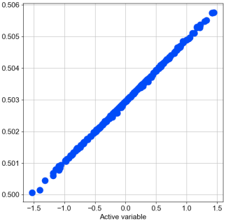
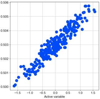
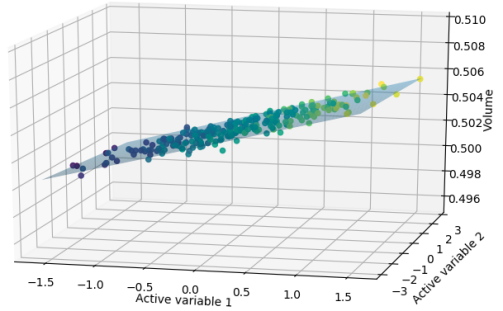
Figure 2: On the left the load volume with respect to the active variable $\bm{\mu}_{\text{vol}}$, while in the center with respect to the shared variable $\bm{\mu}_{Q}$. On the right the shared variable is 2D and there is a response surface of order one.

To capture the most information while having the possibility to plot the results, we select the active subspace to be of dimension 2 for both quantities of interest and we compute the corresponding shared subspace, that is a linear combination of the active subspaces of the two functions. Then we select a lower and an upper bound in which we constraint the load volume. After, we compute the subset of the shared subspace that satisfies such constraint in order to impose it on the total resistance. In Figure 3 we plot on the left the volume against the bidimensional shared variable (seen from above) and in red the realizations of the volume between the imposed bounds. In the center we plot the sufficient summary plot for the total resistance with respect to the shared variables and highlight the simulations that satisfy the volume constraint in red, together with the response surface. We notice that here the data are more scattered if compared with the volume. This is due to the high nonlinearity of the problem and the inactive directions we discarded. On the right we construct a polynomial response surface of order 2 using only the red dots and in green we highlight the minimum of such response surface. That represents the minimum of the total resistance in the reduced parameter space subjected to the volume constraint. The root mean square error committed with the response surface is around 0.7 Newton depending on the run. We can map such reduced point in the full space of the parameters and deform the original hull accordingly. This represents a good starting point for a more sophisticated optimization.

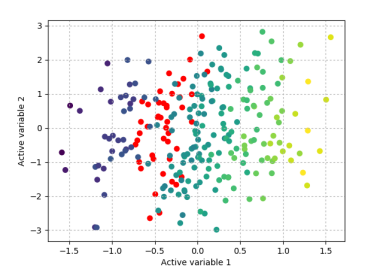
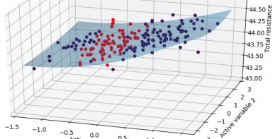
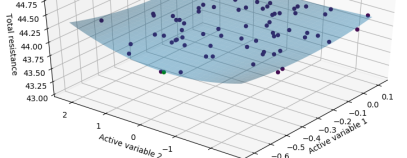
Figure 3: On the left and in the center the sufficient summary plot of the resistance along with a polynomial response surface. In red the points that satisfy the volume constraint. On the right the response surface of order two constructed with the red points. In green the minimum.

8 Conclusions and Perspectives

In this work we presented a complete pipeline composed of shape parametrization, hydrodynamic simulations, and model reduction combining DMD and AS. We applied it to the problem of minimizing the total resistance of a hull advancing in calm water, subject to a load volume constraint, varying the shape of the DTMB 5415. We expressed the two functions in the same reduced space and we constructed a response surface to find the minimum of the total drag that satisfies the volume constraint. We committed an error around 0.7 Newton with respect to the full order solver. This minimum can be used as a starting point of a more sophisticated optimization algorithm. The proposed pipeline is independent of the specific deformed part of the hull, of the solver used, and of the function to minimize. Future work will focus on several different areas to improve physical and mathematical aspects of the algorithms presented, as well as to better integrate its different parts, and to automate the simulation campaign with post processing processes.

References

- [1] PyGeM: Python Geometrical Morphing. https://github.com/mathLab/PyGeM.
- [2] R. F. Beck. Time-domain computations for floating bodies. Applied Ocean Research, 16:267–282, 1994.
- [3] C. A. Brebbia. The Boundary Element Method for Engineers. Pentech Press, 1978.
- [4] P. G. Constantine. Active subspaces: Emerging ideas for dimension reduction in parameter studies, volume 2. SIAM, 2015.
- [5] P. G. Constantine and A. Doostan. Time-dependent global sensitivity analysis with active subspaces for a lithium ion battery model. Statistical Analysis and Data Mining: The ASA Data Science Journal, 10(5):243–262, 2017.
- [6] F. Dassi, A. Mola, and H. Si. Curvature-Adapted Remeshing of CAD Surfaces. In Proceedings of the 23rd International Meshing Roundtable (IMR23), London, Procedia Engineering, pages 253–265, 2014.
- [7] N. Demo, M. Tezzele, A. Mola, and G. Rozza. An efficient shape parametrisation by free-form deformation enhanced by active subspace for hull hydrodynamic ship design problems in open source environment. arXiv preprint arXiv:1801.06369, 2018.
- [8] N. Demo, M. Tezzele, and G. Rozza. PyDMD: Python Dynamic Mode Decomposition. The Journal of Open Source Software, 3(22):530, 2018.
- [9] D. Forti and G. Rozza. Efficient geometrical parametrisation techniques of interfaces for reduced-order modelling: application to fluid–structure interaction coupling problems. International Journal of Computational Fluid Dynamics, 28(3-4):158–169, 2014.
- [10] N. Giuliani, A. Mola, L. Heltai, and L. Formaggia. Engineering Analysis with Boundary Elements FEM SUPG stabilisation of mixed isoparametric BEMs: Application to linearised free surface flows. Engineering Analysis with Boundary Elements, 59:8–22, 2015.
- [11] Z. Grey and P. Constantine. Active subspaces of airfoil shape parameterizations. In 58th AIAA/ASCE/AHS/ASC Structures, Structural Dynamics, and Materials Conference, page 0507, 2017.
- [12] W. Ji, J. Wang, O. Zahm, Y. M. Marzouk, B. Yang, Z. Ren, and C. K. Law. Shared low-dimensional subspaces for propagating kinetic uncertainty to multiple outputs. Combustion and Flame, 190:146–157, 2018.
- [13] J. N. Kutz, S. L. Brunton, B. W. Brunton, and J. L. Proctor. Dynamic Mode Decomposition: Data-Driven Modeling of Complex Systems. SIAM, 2016.
- [14] M. Lombardi, N. Parolini, A. Quarteroni, and G. Rozza. Numerical simulation of sailing boats: Dynamics, FSI, and shape optimization. In Variational Analysis and Aerospace Engineering: Mathematical Challenges for Aerospace Design, page 339. Springer, 2012.
- [15] T. Lukaczyk, F. Palacios, J. J. Alonso, and P. Constantine. Active subspaces for shape optimization. In Proceedings of the 10th AIAA Multidisciplinary Design Optimization Conference, pages 1–18, 2014.
- [16] A. Mola, L. Heltai, and A. De Simone. Wet and Dry Transom Stern Treatment for Unsteady and Nonlinear Potential Flow Model for Naval Hydrodynamics Simulations. Journal of Ship Research, 61(1):1–14, 2017.
- [17] A. Mola, L. Heltai, and A. DeSimone. A stable and adaptive semi-lagrangian potential model for unsteady and nonlinear ship-wave interactions. Engineering Analysis with Boundary Elements, 128–143:37, 2013.
- [18] A. Mola, L. Heltai, and A. Desimone. Ship sinkage and trim predictions based on a CAD interfaced fully nonlinear potential model. In The proceedings of the 26th International Ocean and Polar Engineering Conference, 2016.
- [19] A. Morall. 1957 ITTC Model-ship Correlation Line Values of Frictional Resistance Coefficient. Technical report, National Physical Laboratory, Ship Division, 1970.
- [20] A. Olivieri, F. Pistani, A. Avanzini, F. Stern, and R. Penna. Towing tank experiments of resistance, sinkage and trim, boundary layer, wake, and free surface flow around a naval combatant INSEAN 2340 model. Technical report, DTIC Document, 2001.
- [21] G. Rozza, A. Koshakji, and A. Quarteroni. Free Form Deformation techniques applied to 3D shape optimization problems. Communications in Applied and Industrial Mathematics, 4, 2013.
- [22] F. Salmoiraghi, F. Ballarin, L. Heltai, and G. Rozza. Isogeometric analysis-based reduced order modelling for incompressible linear viscous flows in parametrized shapes. Advanced Modeling and Simulation in Engineering Sciences, 3(1):21, 2016.
- [23] P. J. Schmid. Dynamic mode decomposition of numerical and experimental data. Journal of fluid mechanics, 656:5–28, 2010.
- [24] T. Sederberg and S. Parry. Free-Form Deformation of solid geometric models. In Proceedings of SIGGRAPH - Special Interest Group on GRAPHics and Interactive Techniques, pages 151–159, 1986.
- [25] A. Serani, G. Fasano, G. Liuzzi, S. Lucidi, U. Iemma, E. F. Campana, F. Stern, and M. Diez. Ship hydrodynamic optimization by local hybridization of deterministic derivative-free global algorithms. Applied Ocean Research, 59:115–128, 2016.
- [26] D. Sieger, S. Menzel, and M. Botsch. On shape deformation techniques for simulation-based design optimization. In New Challenges in Grid Generation and Adaptivity for Scientific Computing, pages 281–303. Springer, 2015.
- [27] M. Tezzele, F. Ballarin, and G. Rozza. Combined parameter and model reduction of cardiovascular problems by means of active subspaces and POD-Galerkin methods. arXiv:1711.10884, 2017.
- [28] M. Tezzele, F. Salmoiraghi, A. Mola, and G. Rozza. Dimension reduction in heterogeneous parametric spaces with application to naval engineering shape design problems. arXiv:1709.03298, 2017.