Coupled Kohn-Sham equations for electrons and phonons

Abstract

This work establishes the algebraic structure of the Kohn-Sham equations to be solved in a density formulation of electron and phonon dynamics, including the superconducting order parameter. A Bogoliubov transform is required to diagonalize both the fermionic and bosonic Kohn-Sham Hamiltonians since they both represent a non-interacting quantum field theory. The Bogoliubov transform for phonons is non-Hermitian in the general case, and the corresponding time-evolution is non-unitary. Several sufficient conditions for ensuring that the bosonic eigenvalues are real are provided and a practical method for solving the system is described. Finally, we produce a set of approximate mean-field potentials which are functionals of the electronic and phononic density matrices and depend on the electron-phonon vertex.

In this work we determine time-dependent Kohn-Sham matrix equations used for combined systems of electron and phonons. Ultimately, the potentials which enter the equations are considered to be functionals of the density matrices produced from the time-evolving Kohn-Sham state. One particular aim of this work is to include lattice degrees of freedom in simulations of intense laser pulses acting on solids. This is necessary for the recovery of the magnetic moment or the superconducting order parameter which are typically destroyed by the laser pulse.

I Densities of the electron-nuclear system

Consider the electron-nuclear Schrödinger equation in atomic units:

$$\hat{H}=\frac{1}{2}\sum_{i}\nabla_{i}^{2}+\sum_{I=1}\frac{1}{2M_{I}}\nabla_{I}^{2}+\sum_{i>j}\frac{1}{|{\bf r}_{i}-{\bf r}_{j}|}+\sum_{i,I}\frac{Z_{I}}{|{\bf r}_{i}-{\bf R}_{I}|}+\sum_{I>J}\frac{Z_{I}Z_{J}}{|{\bf R}_{I}-{\bf R}_{J}|}$$ (1)

for $i,j=1\ldots N_{\rm e}$ electrons and $I,J=1\ldots N_{\rm n}$ nuclei, where $M_{I}$ is the nuclear mass and $Z_{I}$ is the nuclear charge, assumed negative. The wave function $\Psi(\underline{\underline{\bf r}},\underline{\underline{s}},\underline{\underline{\bf R}},\underline{\underline{S}},t)$, where $\underline{\underline{s}}$ and $\underline{\underline{S}}$ are electron and nuclear spin coordinates, is determined in a finite (but large) box with periodic boundary conditions.

Conventional densities obtained from this wave function are spatially constant and therefore not useful as variational quantities and a different approach to density functional theory (DFT) is required. The electron-nuclear wave function can be factored exactlyAbedi2010 as:

$$\Psi(\underline{\underline{\bf r}},\underline{\underline{s}},\underline{\underline{\bf R}},\underline{\underline{S}},t)=\Phi_{\underline{\underline{\bf R}},\underline{\underline{S}}}(\underline{\underline{\bf r}},\underline{\underline{s}},t)\chi(\underline{\underline{\bf R}},\underline{\underline{S}},t),$$ (2)

where $\sum_{\underline{\underline{s}}}\int d\underline{\underline{\bf r}}\,|\Phi_{\underline{\underline{\bf R}},\underline{\underline{S}}}(\underline{\underline{\bf r}},\underline{\underline{s}},t)|^{2}=1$ for all $\underline{\underline{\bf R}}$, $\underline{\underline{S}}$ and $t$.

Let $V_{\rm BO}(\underline{\underline{\bf R}})$ be the Born-Oppenheimer (BO) potential energy surface (PES) and suppose this has a unique minimum at $\underline{\underline{\bf R}}^{0}$.

I.1 Electronic densities

A purely electronic wave function is obtained by evaluating $\Phi_{\underline{\underline{\bf R}}^{0}\underline{\underline{S}}}(\underline{\underline{\bf r}},\underline{\underline{s}},t)$. From this, a variety of familiar electronic densities may be obtained, for example

$$\rho_{\underline{\underline{\bf R}}^{0}}({\bf r},t)\equiv\sum_{\underline{\underline{S}}}\int d^{3}r_{2}\ldots d^{3}r_{N_{\rm e}}\left|\Phi_{\underline{\underline{\bf R}}^{0},\underline{\underline{S}}}(\underline{\underline{\bf r}},\underline{\underline{s}},t)\right|^{2},$$ (3)

with similar definitions for the magnetization ${\bf m}({\bf r})$, current density ${\bf j}({\bf r})$, superconducting order parameter, $\chi({\bf r},{\bf r}^{\prime})$ and so on. Such a density is plotted in Fig. 1 for the hydrogen atom using various masses. Note that this density is not a constant and also varies with the nuclear mass. The densities for $M=\infty$ and the physical mass of a proton, $M\simeq 1836$, are indistinguishable. However, the density is considerably different when the nuclear and electronic masses are the same, $M=1$. In the same figure is a plot of the density evaluated at a particular point against $1/M$. The density decreases monotonically with reciprocal mass and has a non-zero derivative at $1/M=0$.

A Kohn-Sham Hamiltonian defined to reproduce the density in (3) as its ground state can be written as

$$\hat{H}_{\rm KS}=-\frac{1}{2}\nabla^{2}+V_{\underline{\underline{\bf R}}^{0}}({\bf r})+V_{\rm H}({\bf r})+V_{\rm xc}({\bf r})+V_{\rm fmc}({\bf r},t),$$ (4)

where $V_{\underline{\underline{\bf R}}^{0}}({\bf r})$ is the external potential determined from the nuclei fixed at $\underline{\underline{\bf R}}^{0}$; $V_{\rm H}$ and $V_{\rm xc}$ are the usual Hartree and exchange-correlation potential; and $V_{\rm fmc}$ is a correction term to account for the finite mass of the nuclei. Note that this potential vanishes in the infinite mass limit, i.e. $\lim_{M\rightarrow\infty}V_{\rm fmc}({\bf r},t)=0$, and the regular Kohn-Sham equations for a fixed external potential are recovered. The finite mass correction potential is plotted in Fig. 1 for hydrogen with an artificially light $M=2$. Not surprisingly, the potential is mainly repulsive. Mass correction potentials corresponding to other densities can also be defined such as a magnetic field ${\bf B}_{\rm fmc}({\bf r},t)$ or a pairing potential $\Delta_{\rm fmc}({\bf r},{\bf r}^{\prime},t)$. In the latter case, the finite mass correction constitutes the entire potential for phonon-coupled superconductors.

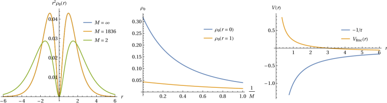
Figure 1: On the left is a plot of the electronic charge density times $r^{2}$, as defined in (3), versus $r$ for various nuclear masses. In the middle is the charge density evaluated at $r=0$ and $r=1$ plotted as a function of $1/M$. On the right is a plot of the finite mass correction potential, evaluated for $M=2$, plotted alongside the nuclear potential $-1/r$.

I.2 Phonon densities

We now consider the expansion of the BO PES around $\underline{\underline{\bf R}}^{0}$ and assume that the leading order, apart from a constant, is quadratic:

$$V_{\rm BO}(\underline{\underline{\bf R}})=V_{\rm BO}(\underline{\underline{\bf R}}^{0})+\frac{1}{2}\sum_{I\alpha,J\beta}u_{I\alpha}K_{I\alpha,J\beta}u_{J\beta}+\cdots$$ (5)

where $K_{I\alpha,J\beta}\equiv\left.\partial^{2}V_{\rm BO}/\partial R_{I\alpha}\partial R_{J\beta}\right|_{\underline{\underline{\bf R}}^{0}}$, $\underline{\underline{\bf u}}\equiv\underline{\underline{\bf R}}-\underline{\underline{\bf R}}^{0}$ and $\alpha$, $\beta$ represent Cartesian directions. The associated classical modes, called phonons, are determined by solving the eigenvalue equation

$$K{\bf e}_{n}=\nu_{n}^{2}M{\bf e}_{n}$$ (6)

for $\nu_{n}$ and ${\bf e}_{n}$, where $M_{I\alpha,J\beta}\equiv M_{I}\delta_{IJ}\delta_{\alpha\beta}$ is the diagonal matrix of nuclear masses. Let $\hat{p}_{I\alpha}\equiv-i\partial_{I\alpha}$ be the momentum operator which acts on a particular nuclear coordinate, then $[\hat{u}_{I\alpha},\hat{p}_{J\beta}]=i\delta_{IJ}\delta_{\alpha\beta}$. We can also define

$$\hat{\mathcal{U}}\equiv\mathcal{S}\hat{\bf u}\qquad\hat{\mathcal{P}}\equiv\mathcal{T}\hat{\bf p},$$ (7)

where $\mathcal{S}=2^{-\frac{1}{2}}\nu^{\frac{1}{2}}{\bf e}^{t}$, $\mathcal{T}=2^{-\frac{1}{2}}\nu^{-\frac{1}{2}}{\bf e}^{t}M^{-1}$ and $\nu$ is the diagonal matrix of eigenvalues, then $[\hat{\mathcal{U}},\hat{\mathcal{P}}]=\frac{i}{2}I$ and $\hat{H}^{\rm b}=\hat{\mathcal{P}}^{t}\nu\hat{\mathcal{P}}+\hat{\mathcal{U}}^{t}\nu\hat{\mathcal{U}}$. Writing

$$\hat{d}=\hat{\mathcal{U}}+i\hat{\mathcal{P}}\qquad\hat{d}^{{\dagger}}=\hat{\mathcal{U}}^{t}-i\hat{\mathcal{P}}^{t},$$ (8)

the Hamiltonian is cast in diagonal form

$$\hat{H}^{\rm b}=\sum_{i}\nu_{i}\left(\hat{d}_{i}^{{\dagger}}\hat{d}_{i}+\frac{1}{2}\right).$$ (9)

We will equate the exact expectation values of nuclear positions, momenta and bilinear combinations thereof with those of a fictitious, non-interacting bosonic system. Thus if the expectation values $\langle\hat{d}_{i}^{{\dagger}}\rangle$ and $\langle\hat{d}_{i}\rangle$ are known, then expectation values of the displacement and momentum operators can be reconstructed from $\langle\hat{\bf u}\rangle=\frac{1}{2}\mathcal{S}^{-1}(\langle\hat{d}^{{\dagger}}\rangle^{t}+\langle\hat{d}\rangle)$ and $\langle\hat{\bf p}\rangle=\frac{i}{2}\mathcal{T}^{-1}(\langle\hat{d}^{{\dagger}}\rangle^{t}-\langle\hat{d}\rangle)$. Bilinear expectation values $\langle\hat{d}_{i}^{{\dagger}}\hat{d}_{j}^{{\dagger}}\rangle$, $\langle\hat{d}_{i}\hat{d}_{j}\rangle$ and $\langle\hat{d}_{i}^{{\dagger}}\hat{d}_{j}\rangle$ can be used to evaluate corresponding products of momentum and position. For instance

$$\langle\hat{\bf u}\otimes\hat{\bf p}\rangle=\frac{i}{4}\mathcal{S}^{-1}\left\langle(\hat{d}^{{\dagger}})^{t}\hat{d}^{{\dagger}}-(\hat{d}^{{\dagger}})^{t}(\hat{d})^{t}-\hat{d}\hat{d}^{{\dagger}}+\hat{d}(\hat{d})^{t}\right\rangle(\mathcal{T}^{-1})^{t}.$$ (10)

Note that in the unperturbed harmonic oscillator ground state, all these expectation values are zero. A further point is that the Hermiticity of the second-quantized bosonic system described below renders some of these expectation values inaccessible, one of which is the nuclear current density. By removing the Hermitian constraint this restriction is lifted.

II Algebraic form of the electron and phonon Kohn-Sham equations

In this section, the details of the Kohn-Sham Hamiltonian, such as that in (4), are removed and we focus on the algebraic structure instead. This is done by considering only the matrix elements of the electron and phonon Hamiltonians. In the following section all matrices are taken to be finite in size.

II.1 Kohn-Sham Hamiltonian for electrons

The most general fermionic Kohn-Sham Hamiltonian of interest here has the form

$$\hat{H}_{s}^{\rm f}=\sum_{i,j=1}^{n_{\rm f}}A_{ij}\hat{a}_{i}^{{\dagger}}\hat{a}_{j}+B_{ij}\hat{a}_{i}^{{\dagger}}\hat{a}_{j}^{{\dagger}}-B_{ij}^{*}\hat{a}_{i}\hat{a}_{j},$$ (11)

where $A$ is a Hermitian matrix representing (4); $B$ is antisymmetric and corresponds to the matrix elements of the superconducting pairing potential $\Delta({\bf r},{\bf r}^{\prime})$. The sum runs to the number of fermionic basis vectors $n_{\rm f}$. The matrix $A$ includes a chemical potential term $A_{ij}\rightarrow A_{ij}+\mu\delta_{ij}$ which is used to fix the total electronic number to $N_{\rm e}$. The Hermitian eigenvalue problem

$$\Bigg{(}\begin{matrix}A&B\\ B^{{\dagger}}&-A^{*}\end{matrix}\Bigg{)}\Bigg{(}\begin{matrix}\vec{U}_{j}\\ \vec{V}_{j}\end{matrix}\Bigg{)}=\varepsilon_{j}\Bigg{(}\begin{matrix}\vec{U}_{j}\\ \vec{V}_{j}\end{matrix}\Bigg{)}$$ (12)

yields $2n_{\rm f}$ solutions. However, if $\varepsilon_{j}$ and $(\vec{U}_{j},\vec{V}_{j})$ are an eigenpair, then so are $-\varepsilon_{j}$ and $(\vec{V}_{j}^{*},\vec{U}_{j}^{*})$. Now we select $n_{\rm f}$ eigenpairs with each corresponding to either a positive or negative eigenvalues but with its conjugate partner not in the set. This choice will not affect the eventual Kohn-Sham ground state. Let $U$ and $V$ be the $n_{\rm f}\times n_{\rm f}$ matrices with these solutions arranged column-wise. Orthogonality of the vectors is then expressed as

$$\Bigg{(}\begin{matrix}\,U\,&\,V^{*}\,\\ \,V\,&\,U^{*}\,\end{matrix}\Bigg{)}^{{\dagger}}\Bigg{(}\begin{matrix}\,U\,&\,V^{*}\,\\ \,V\,&\,U^{*}\,\end{matrix}\Bigg{)}=I,$$ (13)

which implies $U^{{\dagger}}U+V^{{\dagger}}V=I$ and $U^{{\dagger}}V^{*}+V^{{\dagger}}U^{*}=0$. Completeness further implies $UU^{{\dagger}}+V^{*}V^{t}=I$ and $UV^{{\dagger}}+V^{*}U^{t}=0$. The Hamiltonian (11) can now be diagonalized with the aid of $U$ and $V$ via a Bogoliubov transformation:

$$\begin{split}\hat{\alpha}_{j}^{{\dagger}}&=\sum_{i=1}^{n_{\rm f}}U_{ij}\hat{a}_{i}^{{\dagger}}+V_{ij}\hat{a}_{i}\\ \hat{\alpha}_{j}&=\sum_{i=1}^{n_{\rm f}}U_{ij}^{*}\hat{a}_{i}+V_{ij}^{*}\hat{a}_{i}^{{\dagger}},\end{split}$$ (14)

in other words

$$\hat{H}_{s}=\sum_{i=1}^{n_{\rm f}}\varepsilon_{i}\hat{\alpha}_{i}^{{\dagger}}\hat{\alpha}_{i}+W_{0},$$ (15)

where $W_{0}=-{\rm tr}(V\varepsilon V^{{\dagger}})$. The fermionic algebra is also preserved for $\hat{\alpha}$:

$$\bigl{\{}\hat{\alpha}_{i},\hat{\alpha}_{j}^{{\dagger}}\bigr{\}}=\delta_{ij}\qquad\bigl{\{}\hat{\alpha}_{i},\hat{\alpha}_{j}\bigr{\}}=0\qquad\bigl{\{}\hat{\alpha}_{i}^{{\dagger}},\hat{\alpha}_{j}^{{\dagger}}\bigr{\}}=0.$$ (16)

II.1.1 Non-interacting ground state

Given $A$ and $B$, the matrices $U$, $V$ and $\varepsilon$ are fixed by the Kohn-Sham-Bogoliubov equations (12). What remains is to construct from these the eigenstates of (11) in the Fock space. To do so, one first needs to find a normalized vacuum state which is anihilated by all the $\hat{\alpha}_{j}$. Here it is (denoted $|\bar{0}\rangle$ so as to distinguish it from the normal vacuum state $|0\rangle$):

$$|\bar{0}\rangle\equiv\prod_{j=1}^{n_{\rm f}}\hat{U}_{j}\prod_{k=1}^{n_{\rm f}}\hat{a}_{k}^{{\dagger}}|0\rangle+\prod_{j=1}^{n_{\rm f}}\hat{V}_{j}^{{\dagger}}|0\rangle,$$ (17)

where $\hat{U}_{j}\equiv\sum_{i}U_{ij}^{*}\hat{a}_{i}$ and $\hat{V}_{j}^{{\dagger}}\equiv\sum_{i}V_{ij}^{*}\hat{a}_{i}^{{\dagger}}$. It is readily verified that $\hat{\alpha}_{j}|\bar{0}\rangle=0$ for all $j$; the vacuum has the correct normalisation $\langle\bar{0}|\bar{0}\rangle=1$; and the vacuum energy $\langle\bar{0}|H_{s}|\bar{0}\rangle=W_{0}$. The non-interacting many-body ground state can be constructed in analogy with the usual fermionic situation. Let $M$ be the number of $\varepsilon_{j}<0$, then the ground state

$$|\Phi_{0}\rangle=\prod_{j=1}^{M}\hat{\alpha}_{j}^{{\dagger}}|\bar{0}\rangle,$$ (18)

so that

$$\hat{H}_{s}|\Phi_{0}\rangle=E_{0}^{s}|\Phi_{0}\rangle,$$ (19)

where $E_{0}^{s}=\sum_{j=1}^{M}\varepsilon_{j}+W_{0}$.

II.2 Normal and anomalous densities

To determine the densities, both normal and anomalous, one first has to find the expectation values of pairs of $\hat{a}$ and $\hat{a}^{{\dagger}}$. These in turn are linear combinations of expectation values of pairs of $\hat{\alpha}$ and $\hat{\alpha}^{{\dagger}}$. Using the anti-commutation relations (16) and remembering that $\hat{\alpha}|\bar{0}\rangle=0$, we get

$$\langle\Phi_{0}|\hat{\alpha}_{i}^{{\dagger}}\hat{\alpha}_{j}|\Phi_{0}\rangle=\begin{cases}\delta_{ij}&i,j\leq M\\ 0&i,j>M\end{cases}\qquad\langle\Phi_{0}|\hat{\alpha}_{i}\hat{\alpha}_{j}^{{\dagger}}|\Phi_{0}\rangle=\begin{cases}0&i,j\leq M\\ \delta_{ij}&i,j>M\end{cases}$$ (20)

and

$$\langle\Phi_{0}|\hat{\alpha}_{i}^{{\dagger}}\hat{\alpha}_{j}^{{\dagger}}|\Phi_{0}\rangle=0\qquad\langle\Phi_{0}|\hat{\alpha}_{i}\hat{\alpha}_{j}|\Phi_{0}\rangle=0.$$ (21)

Equations (14), (20) and (21) give the normal and anomalous density matrices:

$$\langle\Phi_{0}|\hat{a}_{i}^{{\dagger}}\hat{a}_{j}|\Phi_{0}\rangle=\sum_{k=1}^{M}U_{ik}^{*}U_{jk}+\sum_{k=M+1}^{n_{\rm f}}V_{ik}V_{jk}^{*}$$ (22)

and

$$\langle\Phi_{0}|\hat{a}_{i}^{{\dagger}}\hat{a}_{j}^{{\dagger}}|\Phi_{0}\rangle=\sum_{k=1}^{M}U_{ik}^{*}V_{jk}+\sum_{k=M+1}^{n_{\rm f}}V_{ik}U_{jk}^{*}.$$ (23)

II.2.1 Time evolution

What remains is to determine how the Kohn-Sham state evolves with time in the time-dependent density function theory (TDDFT) version of the method. The form of the ground state equations dictates that of the time-dependent equations. Thus if we assume that the matrices $A$ and $B$ are now functions of time, then the time-dependent generalization of the orbital equation (12) is

$$i\frac{\partial}{\partial t}\Bigg{(}\begin{matrix}\vec{U}_{j}\\ \vec{V}_{j}\end{matrix}\Bigg{)}=\Bigg{(}\begin{matrix}A(t)&B(t)\\ B^{{\dagger}}(t)&-A^{*}(t)\end{matrix}\Bigg{)}\Bigg{(}\begin{matrix}\vec{U}_{j}\\ \vec{V}_{j}\end{matrix}\Bigg{)}$$ (24)

with the Kohn-Sham state given by $|\Phi(t)\rangle=\prod_{i=1}^{M}\hat{\alpha}_{i}^{{\dagger}}(t)|\bar{0}\rangle$. It is easy to show that this state satisfies

$$i\frac{\partial|\Phi(t)\rangle}{\partial t}=\left(\sum_{ij}A_{ij}(t)\hat{a}_{i}^{{\dagger}}\hat{a}_{j}+B_{ij}(t)\hat{a}_{i}^{{\dagger}}\hat{a}_{j}^{{\dagger}}-B_{ij}^{*}(t)\hat{a}_{i}\hat{a}_{j}\right)|\Phi(t)\rangle$$ (25)

with $|\Phi(t=0)\rangle=|\Phi_{0}\rangle$. Note that the number of ‘occupied orbitals’ $M$ remains constant with time. Here we have assumed that the system has evolved from its ground state.

II.3 Kohn-Sham Hamiltonian for phonons

The most general bosonic Kohn-Sham Hamiltonian of interest here has the form

$$\hat{H}_{s}^{\rm b}=\sum_{ij}D_{ij}\hat{d}_{i}^{{\dagger}}\hat{d}_{j}+\tfrac{1}{2}E_{ij}\hat{d}_{i}^{{\dagger}}\hat{d}_{j}^{{\dagger}}+\tfrac{1}{2}E_{ij}^{*}\hat{d}_{i}\hat{d}_{j}+\sum_{i}F_{i}\hat{d}_{i}^{{\dagger}}+F_{i}^{*}\hat{d}_{i},$$ (26)

where $D$ is Hermitian and contains the kinetic energy operator; $E$ is a complex symmetric matrix and $F$ is a complex vector. Note that $\hat{H}_{\rm KS}^{\rm b}$ contains the anomalous terms $\hat{d}_{i}^{{\dagger}}\hat{d}_{j}^{{\dagger}}$ and $\hat{d}_{i}\hat{d}_{j}$. In analogy with the fermionic case, this Hamiltonian can be diagonalized

$$\hat{H}_{s}^{\rm b}=\sum_{i=1}^{n_{\rm b}}\omega_{i}\hat{\gamma}_{i}^{{\dagger}}\hat{\gamma}_{i}+\Omega_{0}$$ (27)

with the Bogoliubov-type transformation

$$\begin{split}\hat{\gamma}_{j}=\sum_{i=1}^{n_{\rm b}}W_{ij}^{*}\hat{d}_{i}+X_{ij}^{*}\hat{d}_{i}^{{\dagger}}+y_{j}^{*}\\ \hat{\gamma}_{j}^{{\dagger}}=\sum_{i=1}^{n_{\rm b}}W_{ij}\hat{d}_{i}^{{\dagger}}+X_{ij}\hat{d}_{i}+y_{j},\end{split}$$ (28)

where $W$ and $X$ are complex matrices and $y$ is a complex vector. The index $j$ runs from $1$ to twice the number of bosonic modes. Requiring that $\hat{\gamma}$ and $\hat{\gamma}^{{\dagger}}$ obey bosonic algebra (the complex numbers $y_{j}$ obviously commute with themselves and the operators, maintaining the algebra) yields

$$W^{{\dagger}}W-X^{{\dagger}}X=I$$ (29)

$$W^{t}X-X^{t}W=0.$$ (30)

After some manipulation, we arrive at the Kohn-Sham-Bogoliubov equations for phonons:

$$\Bigg{(}\begin{matrix}D&-E\\ E^{*}&-D^{*}\end{matrix}\Bigg{)}\Bigg{(}\begin{matrix}\vec{W}_{j}\\ \vec{X}_{j}\end{matrix}\Bigg{)}=\omega_{j}\Bigg{(}\begin{matrix}\vec{W}_{j}\\ \vec{X}_{j}\end{matrix}\Bigg{)}.$$ (31)

The above equation can not be reduced to a symmetric eigenvalue problem because the conditions (29) and (30) correspond to the indefinite inner product $\eta={\rm diag}(1,\ldots,1,-1,\ldots,-1)$. Such matrix Hamiltonians can still possess real eigenvalues Sudarshan1961 ; Mostafazadeh2002 .

II.3.1 Real case

We now consider the special case where the matrices $D$ and $E$ are real symmetric and the vector $F$ is also real. The bosonic Hamiltonian can be written as

$$\hat{H}_{s}^{\rm b}=\sum_{ij}D_{ij}\hat{d}_{i}^{{\dagger}}\hat{d}_{j}+\tfrac{1}{2}E_{ij}\left(\hat{d}_{i}^{{\dagger}}\hat{d}_{j}^{{\dagger}}+\hat{d}_{i}\hat{d}_{j}\right)+\sum_{i}F_{i}\left(\hat{d}_{i}^{{\dagger}}+\hat{d}_{i}\right).$$ (32)

We now prove that under certain conditions, the matrix equation (31) always possesses $n_{\rm b}$ solutions which satisfy (29) and (30). This requires the observation that if the vector $v\equiv(w,x)$ with eigenvalue $\omega$ is a solution to (31), then so is $\bar{v}\equiv(x,w)$ with eigenvalue $-\omega$.

Theorem 1.

Let

$$H=\Bigg{(}\begin{matrix}D&-E\\ E&-D\end{matrix}\Bigg{)},$$

where $D$ and $E$ are real symmetric $n_{\rm b}\times n_{\rm b}$ matrices. Suppose $H$ has only real, non-degenerate eigenvalues and every eigenvector $v$ satisfies $v^{t}\eta v\neq 0$. Then

1. The eigenvectors of $H$ may be chosen real.

2. The eigenvalue equation (31) has exactly $n_{\rm b}$ solutions which satisfy the conditions (29) and (30).

Proof.

The proof that the eigenvectors may be chosen real is straight-forward, so we now prove the second statement. Let $v_{1}$ and $v_{2}$ be two real eigenvectors of $H$ with corresponding real eigenvalues $\omega_{1}$ and $\omega_{2}$. Now $Hv_{1}=\omega_{1}v_{1}\Rightarrow\eta Hv_{1}=\omega_{1}\eta v_{1}$ and because $\eta H$ is symmetric we have $v_{1}^{t}\eta H=\omega_{1}v_{1}^{t}\eta$ and thus $v_{1}^{t}\eta Hv_{2}=\omega_{1}v_{1}^{t}\eta v_{2}$. We also have that $Hv_{2}=\omega_{2}v_{2}$ and so $v_{1}^{t}\eta Hv_{2}=\omega_{2}v_{1}^{t}\eta v_{2}$. Subtracting and using the fact that $\omega_{1}\neq\omega_{2}$ yields $v_{1}^{t}\eta v_{2}=0$. This is equivalent to the off-diagonal part of condition (29). Consider an eigenvector $v=(w,x)$ of $H$. Now $v^{t}\eta v\neq 0$, thus if $v^{t}\eta v<0$ then choose the other eigenvector $\bar{v}$ for which $\bar{v}^{t}\eta\bar{v}>0$. Such an eigenvector can be rescaled arbitrarily to ensure $v^{t}\eta v=1$. This corresponds to the diagonal part of (29) but is valid for only half of the total number of eigenvectors since rescaling cannot change the sign of $v^{t}\eta v$. These remaining vectors are discarded. Condition (30) is trivially satisfied for the diagonal. For any two vectors $v_{i}$ and $v_{j}$ suppose $v_{j}\neq\bar{v}_{i}$ then $\bar{v}_{j}=v_{k}$ for some other $k$. The off-diagonal part of condition (29) is satisfied for all vectors, thus $v_{i}^{t}\eta v_{k}=v_{i}^{t}\eta\bar{v}_{j}=0$. If $v_{j}=\bar{v}_{i}$ then one of these vectors will have been discarded. ∎

The theorem is easily extended to the case where $H$ has degenerate eigenvalues. There is no guarantee that the eigenvalues of $H$ are real since the matrix is not Hermitian. We therefore need additional restrictions on the matrices $D$ and $E$ to ensure this; the following conditions are sufficient but not necessary. We use the notation $P\succ 0$ to mean that the symmetric matrix $P$ is positive definite, and that $P\succ Q$ implies $P-Q\succ 0$.

Theorem 2.

Let $D\succ 0$, and suppose that $E$ is a symmetric matrix. If any of the following are true then $H$ has real eigenvalues:

1. $D\succ ED^{-1}E$.

2. The largest eigenvalue of $(ED^{-1})^{2}$ is less than $1$.

3. $z^{{\dagger}}Dz>|z^{{\dagger}}Ez|$ for all $z\in\mathbb{C}^{n_{\rm b}}$.

4. $E\succ 0$ and $D\succ E$.

5. $E\succ 0$ and $D^{p}\succ E^{p}$, where $p\geq 1$.

6. $D^{2}\succ E^{2}$.

Furthermore, if all eigenvalues are non-zero then all eigenvectors satisfy $v^{t}\eta v\neq 0$.

Proof.

Let $\omega$ and $v$ be an eigenvalue and eigenvector of $H$. The matrix

$$\eta H=\Bigg{(}\begin{matrix}D&-E\\ -E&D\end{matrix}\Bigg{)}$$

is symmetric, therefore both sides of $v^{{\dagger}}\eta Hv=\omega v^{{\dagger}}\eta v$ are real. The only requirement for $\omega$ to be real is that $v^{{\dagger}}\eta Hv$ be non-zero, which is ensured so long as $\eta H\succ 0$. This follows from either of the conditions i or ii (see, for example, Ref. Horn1990 ). Condition iii follows from Theorem 2.1 in Ref Fitzgerald1977 and iv follows immediately. The Löwner-Heinz theorem Zhan2002 reduces condition v to iv. Finally, suppose $D^{2}\succ E^{2}$ where $E$ may not be positive definite. $E$ is symmetric therefore $E^{2}\succ 0$ which means that there exists a symmetric matrix $e\succ 0$ such that $e^{2}=E^{2}$. The Löwner-Heinz theorem implies that $D\succ e$, therefore $z^{{\dagger}}Dz>z^{{\dagger}}ez$ for all complex vectors $z\in\mathbb{C}^{n_{\rm b}}$. $E$ and $e$ can be simultaneously diagonalized and for each eigenvalue $\lambda$ of $E$ there is a corresponding positive eigenvalue $|\lambda|$ of $e$. In this eigenvector basis, it is easy to see that $z^{{\dagger}}ez\geq|z^{{\dagger}}Ez|$ for all $z$ which in turn gives condition iii, thereby proving vi. In fact, all of the above conditions imply Fitzgerald1977 that $\eta H\succ 0$. Thus if all eigenvalues $\omega\neq 0$ then $v^{t}\eta v\neq 0$. ∎

Corollary 2.1.

Let $D_{0}\succ 0$ and $E\succeq 0$ (positive semi-definite) then $D=D_{0}+E$ yields real eigenvalues for $H$.

Theorem 3.

Let $D$ be an arbitrary real symmetric matrix and let $f$ be a real function such that $|f(x)|<|x|$ for all $x\in\mathbb{R}$, then by setting $E=f(D)$ (in the usual ‘function of matrices’ sense Rinehart1955 ) $H$ has real eigenvalues and every eigenvector $v$ satisfies $v^{t}\eta v\neq 0$.

Proof.

We first note that

$$H^{2}=\Bigg{(}\begin{matrix}D^{2}-E^{2}&[E,D]\\ [E,D]&D^{2}-E^{2}\end{matrix}\Bigg{)}.$$

It is obvious for any $E=f(D)$ that $[E,D]=0$ and $D^{2}\succ E^{2}$. Therefore all the eigenvalues of $H^{2}$ are real and positive. We conclude that the eigenvalues of $H$ are real and non-zero, thus $v^{t}\eta v\neq 0$ follows from Theorem 2. ∎

Theorem 4.

Let $D$ be a real symmetric matrix which has no zero eigenvalues and which commutes with all the matrices in a group representation $S=\{S_{i}\}$. Further suppose that any degenerate eigenvalues of $D$ correspond only to irreducible representations of $S$ (i.e. there are no accidental degeneracies). If $E$ is a real symmetric matrix which also commutes with all the matrices in $S$ then there exists a $\xi>0$ such that if $E\rightarrow\xi E$ then $H(\xi)$ has real eigenvalues.

Proof.

From the properties of the determinant applied to blocked matrices, the eigenvalues of $H^{2}$ are also the eigenvalues of $Q\coloneqq D^{2}-E^{2}+[E,D]$. Since $[D,S_{i}]=[E,S_{i}]=0$ for all $i$ then $D^{2}$, $E^{2}$, $[E,D]$ and thus $Q(\xi)$ also commute with $S_{i}$. Schur’s lemma applies equally well to non-Hermitian matrices therefore the degeneracies of $Q(\xi)$ are not lost as $\xi$ increases. We also note that the roots of a polynomial depend continuously on its coefficients and hence the eigenvalues of $Q(\xi)$ depend continuously on $\xi$. From the conjugate root theorem, if $Q(\xi)$ has a complex eigenvalue then it must also have its complex conjugate as an eigenvalue. For sufficiently small $\xi>0$ the eigenvalues of $D^{2}$ cannot become complex because this would require lifting of a degeneracy. Also because of continuity and because $D^{2}$ has strictly positive eigenvalues, a sufficiently small $\xi>0$ will keep them positive. Hence the eigenvalues of $H(\xi)$ are real. ∎

Once these equations are solved, the vector $y$ is determined from

$$y=\omega^{-1}\left(W^{t}-X^{t}\right)F,$$ (33)

where $\omega={\rm diag}(\omega_{1},\ldots,\omega_{n_{\rm b}})$. The constant term in (27) given by

$$\Omega_{0}=-{\rm tr}\left(X\omega X^{{\dagger}}\right)-y^{{\dagger}}\omega y.$$ (34)

II.3.2 Existence and nature of the vacuum state

We now show that the state which is annihilated by all the $\hat{\gamma}_{i}$ exists. Let

$$\hat{w}_{j}\coloneqq\sum_{i=1}^{n_{\rm b}}W_{ij}^{*}\hat{d}_{i}\qquad\hat{x}_{j}^{{\dagger}}\coloneqq\sum_{i=1}^{n_{\rm b}}X_{ij}^{*}\hat{d}_{i}^{{\dagger}}$$ (35)

then

$$\left[\hat{w}_{j},\hat{x}_{j}^{{\dagger}}\right]=\sum_{i=1}^{n_{\rm b}}W_{ij}^{*}X_{ij}^{*}\eqqcolon\tau_{j}.$$ (36)

Now consider the eigenvalue equation

$$\left(\hat{w}_{j}+\hat{x}_{j}^{{\dagger}}\right)|\bar{0}_{j}\rangle=-y_{j}^{*}|\bar{0}_{j}\rangle.$$ (37)

Using the ansatz

$$|\bar{0}_{j}\rangle=\sum_{n=0}^{\infty}\frac{\kappa_{n}^{j}}{n!}(\hat{x}_{j}^{{\dagger}})^{n}|0\rangle,$$ (38)

we obtain a recurrence relation

$$\kappa_{n}^{j}=\left[-y_{j}^{*}\kappa_{n-1}^{j}-(n-1)\kappa_{n-2}^{j}\right]/\tau_{j}$$ (39)

with $y_{j}^{*}\kappa_{0}^{j}=-\kappa_{1}^{j}\tau_{j}$ and $\kappa_{0}^{j}$ chosen so that $\langle\bar{0}_{j}|\bar{0}_{j}\rangle=1$. Note that if $\kappa_{n}^{j}=1$ for all $n$ then (38) is a coherent state. The vacuum state

$$|\bar{0}\rangle=\zeta\hat{S}\bigotimes_{j=1}^{n_{\rm b}}|\bar{0}_{j}\rangle,$$ (40)

where $\zeta$ is a normalization constant and $\hat{S}$ is the symmetrizing operator, is annihilated by all $\hat{\gamma}_{j}$ and, because $\omega_{j}>0$ for all $j$, is also the bosonic Kohn-Sham ground state, which is the lowest energy Fock space eigenstate of (26), as required.

II.3.3 Phononic observables and time evolution

To make the theory useful, observables which are products of the original $c_{i}$ and $c_{i}^{{\dagger}}$ operators have to be computed. After some straight-forward algebra one finds that linear operators may be evaluated using

$$Y_{i}\coloneqq\langle\bar{0}|\hat{d}_{i}|\bar{0}\rangle=\langle\bar{0}|\hat{d}_{i}^{{\dagger}}|\bar{0}\rangle^{*}=\sum_{j=1}^{n_{\rm b}}X_{ij}^{*}y_{j}-W_{ij}y_{j}^{*}.$$ (41)

Observables which are quadratic are more complicated:

$$\begin{split}\langle\bar{0}|\hat{d}_{i}^{{\dagger}}\hat{d}_{j}|\bar{0}\rangle=Y_{i}^{*}Y_{j}+\left(XX^{{\dagger}}\right)_{ij}\qquad\langle\bar{0}|\hat{d}_{i}\hat{d}_{j}^{{\dagger}}|\bar{0}\rangle=Y_{i}Y_{j}^{*}+\left(WW^{{\dagger}}\right)_{ij}\\ \langle\bar{0}|\hat{d}_{i}^{{\dagger}}\hat{d}_{j}^{{\dagger}}|\bar{0}\rangle=Y_{i}^{*}Y_{j}^{*}-\left(XW^{{\dagger}}\right)_{ij}\qquad\langle\bar{0}|\hat{d}_{i}\hat{d}_{j}|\bar{0}\rangle=Y_{i}Y_{j}-\left(WX^{{\dagger}}\right)_{ij}.\end{split}$$ (42)

The extension to the time-dependent case follows the same procedure as that for fermions, namely that the matrices and vector $D$, $E$ and $F$ in (26) become time-dependent as, consequently, do $\hat{\gamma}_{i}^{{\dagger}}$ and $|\bar{0}\rangle$ after solving the equation of motion

$$i\frac{\partial}{\partial t}\Bigg{(}\begin{matrix}\vec{W}_{j}\\ \vec{X}_{j}\end{matrix}\Bigg{)}=\Bigg{(}\begin{matrix}D(t)&-E(t)\\ E^{*}(t)&-D^{*}(t)\end{matrix}\Bigg{)}\Bigg{(}\begin{matrix}\vec{W}_{j}\\ \vec{X}_{j}\end{matrix}\Bigg{)}.$$ (43)

This time evolution is not unitary but rather pseudo-unitary Mostafazadeh2002b and will not preserve ordinary vector lengths in general but will preserve the indefinite inner product. The vector $y$ can be determined analogously from

$$i\frac{\partial y}{\partial t}=\left(W^{t}(t)-X^{t}(t)\right)F(t).$$ (44)

Evolving (43) and (44) in time is equivalent to doing the same for the second-quantized Hamiltonian and the Fock space state vector:

$$i\frac{\partial|\Psi(t)\rangle}{\partial t}=\left(\sum_{ij}D_{ij}(t)\hat{d}_{i}^{{\dagger}}\hat{d}_{j}+\tfrac{1}{2}E_{ij}(t)\hat{d}_{i}^{{\dagger}}\hat{d}_{j}^{{\dagger}}+\tfrac{1}{2}E_{ij}^{*}(t)\hat{d}_{i}\hat{d}_{j}+\sum_{i}F_{i}(t)\hat{d}_{i}^{{\dagger}}+F_{i}^{*}(t)\hat{d}_{i}\right)|\Psi(t)\rangle.$$ (45)

II.3.4 Numerical aspects

In order to determine the phonon ground state or perform time-evolution with (43) for real systems, we require a numerical algorithm for finding the eigenvalues and eigenvectors of (31). This is not a symmetric or Hermitian problem and while a general non-symmetric eigenvalue solver could be employed, a simple modification of Jacobi’s method can be used to diagonalize the matrix efficiently.

Let $G(i,j,\theta)$ be a Givens rotation matrix, i.e. for $i<j$, $G_{kk}=1$ for $k\neq i,j$, $G_{kk}=\cos\theta$ for $k=i,j$, $G_{ji}=-G_{ij}=\sin\theta$ and zero otherwise. Further define the hyperbolic Givens rotation, $G^{\rm h}(i,j,\theta)$, which is the same except that $G_{kk}=\cosh\theta$ and $G_{ji}=G_{ij}=\sinh\theta$. The Givens and hyperbolic Givens rotations can be combined to diagonalize the matrix in (31). For $i<j$ where $1<j\leq 2N_{\rm b}$ we can define a combined Givens rotation, $G^{\rm c}(i,j,\theta)$, as $G^{\rm c}=G^{\rm h}$ for $i\leq N_{\rm b}$ and $j>N_{\rm b}$; and $G^{\rm c}(i,j,\theta)=G(i,j,\theta)G(i+N_{\rm b},j+N_{\rm b},\theta)$ for $i,j\leq N_{\rm b}$.

Definition 1.

A pair of real, symmetric matrices $A$, $B$ is called positive definite if there exists a real $\mu$ such that $A-\mu B$ is positive definite.

Theorem 5.

Let $\eta H$ and $\eta$ be a positive definite pair. Then applying the combined Givens rotations to $H$ with row-cyclic strategy results in convergence to a diagonal matrix.

See Veselićveselic93 for proof.

II.3.5 Solids

Solid state calculations normally use periodic boundary conditions and Bloch orbitals. Phonon displacements are of the form

$$\mathcal{U}_{n{\bf q}}({\bf R})=N_{q}^{-1/2}2^{-\frac{1}{2}}\nu^{\frac{1}{2}}{\bf e}_{n{\bf q}}e^{i{\bf q}\cdot{\bf R}},$$ (46)

where ${\bf q}$ is a reciprocal lattice vector, $\alpha$ labels a phonon branch, ${\bf R}$ is a primitive lattice vector and ${\bf e}_{n{\bf q}}$ is determined along with $\nu_{n{\bf q}}$ by solving (6) for each ${\bf q}$-vector individually. These displacements are thus complex-valued but by noting that $\nu_{n-{\bf q}}=\nu_{n{\bf q}}$ and ${\bf e}_{n-{\bf q}}={\bf e}_{n{\bf q}}^{*}$ we can form their real-valued counterparts

$$\mathcal{U}_{n{\bf q}}^{(+)}({\bf R})=\frac{1}{\sqrt{2}}\left(\mathcal{U}_{n{\bf q}}({\bf R})+\mathcal{U}_{n-{\bf q}}({\bf R})\right)\qquad\mathcal{U}_{n{\bf q}}^{(-)}({\bf R})=\frac{-i}{\sqrt{2}}\left(\mathcal{U}_{n{\bf q}}({\bf R})-\mathcal{U}_{n-{\bf q}}({\bf R})\right).$$

These are the displacements to which $\hat{d}_{i}$ and $\hat{d}_{i}^{{\dagger}}$ refer and will thus keep the phonon Hamiltonian in (32) real. An approximate electron-phonon vertex is obtained as a by-product of a phonon calculation:

$$\Gamma_{i{\bf k}+{\bf q},j{\bf k},n{\bf q}}=\frac{1}{2}\langle\varphi_{j{\bf k}+{\bf q}}|\partial\hat{V_{s}}/\partial\mathcal{U}_{n{\bf q}}|\varphi_{i{\bf k}}\rangle$$ (47)

where $\hat{V_{s}}$ is the Kohn-Sham potential and the derivative is with respect to the magnitude of the displacement in (46). This is not Hermitian in the indices $i$ and $j$ because the potential derivative corresponds to a complex displacement. The vertex associated with $\mathcal{U}_{n{\bf q}}^{(\pm)}$ has the form

$$\bordermatrix{&{\bf k}-{\bf q}&{\bf k}&{\bf k}+{\bf q}\cr{\bf k}-{\bf q}&0&\Gamma_{n-{\bf q}}&0\cr{\bf k}&\Gamma_{n-{\bf q}}^{{\dagger}}&0&\Gamma_{n{\bf q}}\cr{\bf k}+{\bf q}&0&\Gamma_{n{\bf q}}^{{\dagger}}&0}$$ (48)

which is a Hermitian matrix for all ${\bf q}$ and $n$.

One final point regarding solids is the requirement of keeping the electronic densities lattice periodic. This implies that the potentials $A$ and $B$ should only couple the Bloch vector ${\bf k}$ with itself.

III Mean-field functionals

The final (and possibly most difficult) step in this theory is the determination of potentials represented by the matrices $A$, $B$, $D$, $E$ and vector $F$. In principle, these are chosen to reproduce the exact conditional density $\rho_{\underline{\underline{\bf R}}^{0}}({\bf r},t)$ in (3) as well as the phononic expectation values $\langle\hat{d}_{i}\rangle$, $\langle\hat{d}_{i}^{{\dagger}}\hat{d}_{j}\rangle$, etc., which themselves reproduce exact nuclear positions, momenta and so on. In practice, these potentials need to be approximated and here we will employ a simple mean-field approach by considering the lowest order diagrams which enter the self-energy. These are plotted in Fig. 2 and involve the normal and anomalous, Kohn-Sham electronic Green’s functions $i\mathcal{G}_{ij}(t,t^{\prime})=\langle\Phi_{0}|T[\hat{a}_{i}(t)\hat{a}_{j}^{{\dagger}}(t^{\prime})]|\Phi_{0}\rangle$ and $i\mathcal{F}_{ij}(t,t^{\prime})=\langle\Phi_{0}|T[\hat{a}_{i}^{{\dagger}}(t)\hat{a}_{j}^{{\dagger}}(t^{\prime})]|\Phi_{0}\rangle$, etc., as well as the phonon propagators $i\mathcal{C}_{i}(t)=\langle\bar{0}|\hat{d}_{i}^{{\dagger}}(t)|\bar{0}\rangle$, etc. and $i\mathcal{D}_{ij}(t,t^{\prime})=\langle\bar{0}|T[\hat{d}_{i}(t)\hat{d}_{j}^{{\dagger}}(t^{\prime})]|\bar{0}\rangle$, etc. These quantities are evaluated around their respective Kohn-Sham ground states, (18) and (40). The quantity $A_{0}$ is given by the matrix elements of the single particle Hamiltonian in (4) without $V_{\rm fmc}$, and $D_{0}=\nu$.

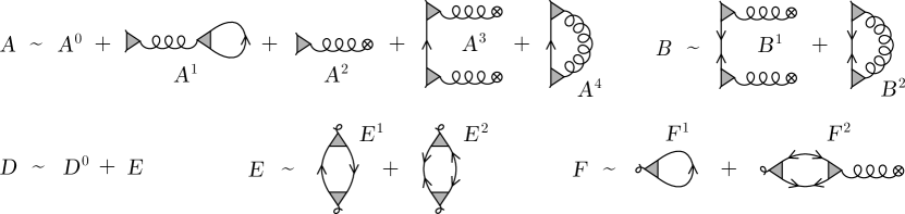
Figure 2: The lowest order contributions to the self-energy from the vertex $\Gamma=\raisebox{-2.0pt}{\mbox{\includegraphics[height=11.0pt]{Gamma.pdf}}}$, the normal and anomalous Green’s functions $\mathcal{G}={\mbox{\includegraphics[height=6.0pt]{G.pdf}}}$ and $\mathcal{F}={\mbox{\includegraphics[height=6.0pt]{F.pdf}}}$, and the phonon propagators $\mathcal{C}={\mbox{\includegraphics[height=7.0pt]{C.pdf}}}$ and $\mathcal{D}={\mbox{\includegraphics[height=7.0pt]{D.pdf}}}$. These are evaluated in the static limit as mean-field potentials for $A$, $B$, $D$, $E$ and $F$.

Explicit expressions for the potentials are found by substituting instantaneous densities or density matrices of the electrons and phonons for the retarded correlation functions in the diagrams. For example, the electronic state would be affected by the phonon system via the expectation values of the phonon operators, yielding a contribution to $A$:

$$A_{ij}^{2}(t)=\sum_{k}\Gamma_{ijk}\left(\langle\hat{d}_{k}^{{\dagger}}\rangle_{t}+\langle\hat{d}_{k}\rangle_{t}\right),$$ (49)

where the expectation values are evaluated with (41) and $\Gamma_{ijk}$ is shorthand for the vertex in (48). At first glance, the matrix $A^{3}$ appears to be an improper part of the self-energy which is already accounted for by $A^{2}$. Such a term is still valid for solids with since $A^{2}$ can only ever couple ${\bf k}$ with itself. However, the Green’s function line in $A^{3}$ can carry momentum ${\bf q}\neq 0$ and yet have the potential preserve lattice periodicity.

The mean-field potential that gives rise to superconductivity is a little more complicated:

$$B_{ij}^{2}(t)=-\sum_{klmn}\Gamma_{ikl}\Gamma_{mjn}\left(\langle\hat{a}_{m}^{{\dagger}}\hat{a}_{k}^{{\dagger}}\rangle_{t}+\langle\hat{a}_{m}\hat{a}_{k}\rangle_{t}\right)\left(\langle\hat{d}_{l}^{{\dagger}}\hat{d}_{n}^{{\dagger}}\rangle_{t}+\langle\hat{d}_{l}^{{\dagger}}\hat{d}_{n}\rangle_{t}+\langle\hat{d}_{l}\hat{d}_{n}^{{\dagger}}\rangle_{t}+\langle\hat{d}_{l}\hat{d}_{n}\rangle_{t}\right),$$ (50)

where the density matrices are determined from (23) and (42). The potential represented by $F$ would be

$$F_{k}^{1}(t)=\sum_{ij}\Gamma_{ijk}\gamma_{ij}(t)$$ (51)

where $\gamma_{ij}(t)=\langle\hat{a}_{i}^{{\dagger}}\hat{a}_{j}\rangle_{t}$ is the electronic one-reduced density matrix calculated using (22). The matrix $E^{1}$ is evaluated as:

$$E_{ij}^{1}(t)=\sum_{klmn}\Gamma_{kli}\Gamma_{mnj}\gamma_{kn}(t)\gamma_{ml}(t).$$ (52)

This matrix should be positive semi-definite in order to satisfy Corollary 2.1 and guarantee real eigenvalues for the bosonic Hamiltonian in (32).

Lemma 6.

The matrix $E^{1}$ is positive semi-definite.

Proof.

We first note that $\Gamma_{kli}=\Gamma_{lki}^{*}$ for all $i$, i.e. $\Gamma$ is Hermitian in the electronic indices. Since $\Gamma_{kli}\Gamma_{mnj}\gamma_{kn}\gamma_{ml}$ and $\Gamma_{lki}\Gamma_{nmj}\gamma_{lm}\gamma_{nk}=\Gamma_{kli}^{*}\Gamma_{mnj}^{*}\gamma_{ml}^{*}\gamma_{kn}^{*}$ both appear in the sum in (52) then $E^{1}$ must be real and symmetric. Let $v$ be a real vector of the same dimension as $E^{1}$, then $R_{kl}\equiv\sum_{i}v_{i}\Gamma_{kli}$ is also Hermitian. The quantity $s\equiv v^{t}E^{1}v$ can be written as $s={\rm tr}(R^{{\dagger}}\gamma R^{{\dagger}}\gamma)$. Let $U$ be the unitary transformation that diagonalizes $\gamma$ and define ${\rm diag}(\tilde{\gamma})\equiv U^{{\dagger}}\gamma U$ and $\tilde{R}\equiv U^{{\dagger}}RU$, then $s={\rm tr}(\tilde{R}^{{\dagger}}\tilde{\gamma}\tilde{R}^{{\dagger}}\tilde{\gamma})$ is left invariant. One of the $N$-representable propertiescoleman63 of $\gamma$ is that its eigenvalues satisfy $0\leq\tilde{\gamma}_{i}\leq 1$. Then $s=\sum_{kl}|\tilde{R}_{kl}|^{2}\tilde{\gamma}_{k}\tilde{\gamma}_{l}\geq 0$. Since $v$ was chosen arbitrarily we conclude that $E^{1}$ is positive semi-definite. ∎

IV Summary

We have defined Kohn-Sham equations for fermions and bosons which are designed to reproduce conditional electronic densities as well as expectation values of the phonon creation and annihilation operators. Sufficient conditions which guarantee real eigenvalues for the bosonic system were found. In practice, the potential matrix elements $A$, $B$, $D$, $E$ and $F$ can be approximated using mean-field potentials inspired from a diagrammatic expansion of the self-energy. The electron and phonon density matrices are determined either self-consistently in a ground state calculation or via simultaneous propagation in the time-dependent case. Any solution obtained in this way is thus non-perturbative. These equations can be implemented in both finite and solid-state codes using quantities determined from linear-response phonon calculations.

References

- [1] Ali Abedi, Neepa T. Maitra, and E. K. U. Gross. Phys. Rev. Lett., 105:123002, 2010.
- [2] E. C. G. Sudarshan. Phys. Rev., 123:2183, 1961.
- [3] A. Mostafazadeh. J. Math. Phys., 43(1):205, 2002.
- [4] R. A. Horn and C. R. Johnson. Matrix Analysis. Cambridge University Press, Cambridge, 1990.
- [5] C. H. Fitzgerald and R. A. Horn. J. London Math. Soc., 15:419, 1977.
- [6] X. Zhan. Matrix Inequalities. Springer-Verlag, Berlin, 2002.
- [7] R. F. Rinehart. Amer. Math. Monthly, 62:395, 1955.
- [8] A. Mostafazadeh. arXiv:math-ph/0302050, 2002.
- [9] K. Veselic. Numer. Math., 64:241, 1993.
- [10] A. J. Coleman. Rev. Mod. Phys., 35:668, 1963.
- [11] J. H. P. Colpa. Physica A, 93:327, 1978.