Sparse Reduced Rank Regression With Nonconvex Regularization

Abstract

In this paper, the estimation problem for sparse reduced rank regression (SRRR) model is considered. The SRRR model is widely used for dimension reduction and variable selection with applications in signal processing, econometrics, etc. The problem is formulated to minimize the least squares loss with a sparsity-inducing penalty considering an orthogonality constraint. Convex sparsity-inducing functions have been used for SRRR in literature. In this work, a nonconvex function is proposed for better sparsity inducing. An efficient algorithm is developed based on the alternating minimization (or projection) method to solve the nonconvex optimization problem. Numerical simulations show that the proposed algorithm is much more efficient compared to the benchmark methods and the nonconvex function can result in a better estimation accuracy.

I Introduction

Reduced Rank Regression (RRR) [1, 2] is a multivariate linear regression model, where the coefficient matrix has a low-rank property. The name of “reduced rank regression” was first brought up by Izenman [3]. Denote the response (or dependent) variables by $\mathbf{y}_{t}\in\mathbb{R}^{P}$ and predictor (or independent) variables by $\mathbf{x}_{t}\in\mathbb{R}^{Q}$, a general RRR model is given as follows:

$$\mathbf{y}_{t}=\boldsymbol{\mu}+\mathbf{A}\mathbf{B}^{T}\mathbf{x}_{t}+\boldsymbol{\varepsilon}_{t},$$ (1)

where the regression parameters are $\boldsymbol{\mu}\in\mathbb{R}^{P}$, $\mathbf{A}\in\mathbb{R}^{P\times r}$ and $\mathbf{B}\in\mathbb{R}^{Q\times r}$ and $\boldsymbol{\varepsilon}_{t}$ is the model innovation. Matrix $\mathbf{A}$ is often called sensitivity (or exposure) matrix and $\mathbf{B}$ is called factor matrix with the linear combinations $\mathbf{B}^{T}\mathbf{x}_{t}$ called latent factors. The “low-rank structure” formed by $\mathbf{A}\mathbf{B}^{T}$ essentially reduces the parameter dimension and improves explanatory ability of the model. The RRR model is widely used in situations when the response variables are believed to depend on a few linear combinations of the predictor variables, or when such linear combinations are of special interest.

The RRR model has been used in many signal processing problems, e.g., array signal processing [4], state space modeling [5], filter design [6], channel estimation and equalization for wireless communication [7, 8, 9], etc. It is also widely applied in econometrics and financial economics. Problems in econometrics were also the motivation for the pioneering work on the RRR estimation problem [1]. In financial economics, it can be used when modeling a group of economic indices by the lagged values of a set of economic variables. It is also widely used to model the relationship between financial asset returns and some related explanatory variables. Several asset pricing theories have been proposed for testing the efficiency of portfolios [10] and empirical verification using asset returns data on industry portfolios has been made through tests for reduced rank regression [11]. The RRR model is also closely related the vector error correction model [12] in time series modeling and the latent factors can be used for statistical arbitrage [13] in finance. More applications on the RRR model can be found in, e.g., [14].

Like the low-rank structure for factor extraction, row-wise group sparsity on matrix $\mathbf{B}$ can also be considered to further realize predicting variable selection, which leads to the sparse RRR (SRRR) model [15]. Since $\mathbf{B}^{T}\mathbf{x}_{t}$ can be interpreted as the linear factors linking the response variables and the predictors, the SRRR can generate factors only with a subset of all the predictors. Variable selection is very important target in data analytics since it can help with model interpretability and improve estimation and forecasting accuracy.

In [15], the authors first considered the SRRR estimation problem, where the group sparsity was induced via the group lasso penalty [16]. An algorithm based on the alternating minimization (AltMin) method [17] was proposed. However, the proposed algorithm has a double loop where subgradient or variational method is used for the inner problem solving. Such an algorithm can be very slow in practice due to the double-loop nature where lots of iterations may be necessary to get an accurate enough solution at each iteration. Apart from that, besides the convex function for sparsity inducing, it is generally acknowledged that a nonconvex sparsity-inducing function can attain a better performance [18] which is proposed to use for sparsity estimation in this paper.

In this paper, the objective of the SRRR estimation problem is given as the ordinary least squares loss with a sparsity-inducing penalty. An orthogonality constraint is added for model identification purpose [15]. To solve this problem, an efficient AltMin-based single-loop algorithm is proposed. In order to pursue low-cost updating steps, a majorization-minimization method [19] and a nonconvexity redistribution method [20] are further adopted making the variable updates become two closed-form projections. Numerical simulations show that the proposed algorithm is more efficient compared to the benchmarks and the nonconvex function can attain a better estimation accuracy.

II Sparse Reduced Rank Regression

The SRRR estimation problem is formulated as follows:

$$\begin{array}[]{ll}\underset{\mathbf{A},\mathbf{B}}{\mathsf{minimize}}&F\left(\mathbf{A},\mathbf{B}\right)\triangleq L\left(\mathbf{A},\mathbf{B}\right)+R\left(\mathbf{B}\right)\\ \mathsf{subject\>to}&\mathbf{A}^{T}\mathbf{A}=\mathbf{I},\end{array}$$ (2)

where $L\left(\mathbf{A},\mathbf{B}\right)$ is sample loss function and $R\left(\mathbf{B}\right)$ is the row-wise group sparsity regularizer. The constraint $\mathbf{A}^{T}\mathbf{A}=\mathbf{I}$ is added for identification purpose to deal with the unitary invariance of the parameters [15]. We further assume a sample path $\left\{\mathbf{y}_{t},\mathbf{x}_{t}\right\}_{t=1}^{N}$ $\left(N\geq\max\left(P,Q\right)\right)$ is available from (1).

The least squares loss $L\left(\mathbf{A},\mathbf{B}\right)$ for the RRR model is obtained by minimizing a sample $\ell_{2}$-norm loss as follows:

$$\begin{array}[]{c}L\left(\mathbf{A},\mathbf{B}\right)=\frac{1}{2}\sum_{t=1}^{N}\left\|\mathbf{y}_{t}-\mathbf{A}\mathbf{B}^{T}\mathbf{x}_{t}\right\|_{2}^{2}\\ \quad\quad=\frac{1}{2}\left\|\mathbf{Y}-\mathbf{A}\mathbf{B}^{T}\mathbf{X}\right\|_{F}^{2},\end{array}$$ (3)

where $\mathbf{Y}=\left[\mathbf{y}_{1},\ldots,\mathbf{y}_{N}\right]$ and $\mathbf{X}=\left[\mathbf{x}_{1},\ldots,\mathbf{x}_{N}\right]$.

Sparse optimization [21] has become the focus of much research interest as a way to to realize the variable selection (e.g., the group lasso method). For a vector $\mathbf{x}\in\mathbb{R}^{K}$, the sparsity level is usually measured by the $\ell_{0}$-norm, i.e., $\left\|\mathbf{x}\right\|_{0}=\sum_{i=1}^{K}\mathrm{sgn}\left(\left|x_{i}\right|\right)$. Practically, the $\ell_{1}$-norm is used as the tightest convex relaxation to approximate it as in [15]. Although it is easy for optimization and has been shown to favor sparser solutions, the $\ell_{1}$-norm can lead to biased estimation with solutions not as accurate and sparse as desired and produce inferior prediction performance [18]. Nonconvex regularizers sacrifice convexity but can have a tighter approximation performance and are proposed for sparsity inducing which outperform the convex $\ell_{1}$-norm. In this paper, two nonsmooth sparsity-inducing functions denoted by $\rho\left(\left|x\right|\right)$ are considered: the nonconvex Geman function [22] and the convex $\ell_{1}$-norm. Then, the row-wise group sparsity regularizer $R\left(\mathbf{B}\right)$ induced by $\rho\left(\left|x\right|\right)$ is given as follows:

$$\begin{array}[]{c}R\left(\mathbf{B}\right)=\sum_{i=1}^{Q}\xi_{i}\rho\left(\left\|\mathbf{b}_{i}\right\|_{2}\right),\end{array}$$ (4)

where $\mathbf{b}_{i}$ denotes the $i$th row of $\mathbf{B}$ and $\rho\left(\left|x\right|\right)$ is from $\rho_{\mathrm{GM}}\left(\left|x\right|\right)=\frac{\left|x\right|}{\theta+\left|x\right|}$ ($\theta>0$) and $\rho_{\ell_{1}}\left(\left|x\right|\right)=\left|x\right|$, which are shown in Figure 1.

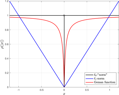
Figure 1: The $\ell_{0}$-”norm” $\left\|x\right\|_{0}\triangleq\mathrm{sgn}\left(x\right)$, $\ell_{1}$-norm $\rho_{\ell_{1}}\left(\left|x\right|\right)\triangleq\left|x\right|$, and nonconvex nonsmooth sparsity-inducing function $\rho\left(\left|x\right|\right)$.

Based on $L\left(\mathbf{A},\mathbf{B}\right)$ and $R\left(\mathbf{B}\right)$, the problem in (2) is a nonconvex nonsmooth optimization problem due to the nonconvex nonsmooth objective and the nonconvex constraint set.

III Problem Solving Based on Alternating Minimization

The objective function in problem (2) has two variable blocks $\left(\mathbf{A},\mathbf{B}\right)$. In this section, an alternating minimization (a.k.a. two-block coordinate descent) algorithm [17] will be proposed to solve it. At the $\left(k+1\right)$th iteration, this algorithm updates the variables according to the following two steps:

$$\begin{cases}\begin{array}[]{l}\mathbf{A}^{\left(k+1\right)}\leftarrow\arg\underset{\mathbf{A}:\mathbf{A}^{T}\mathbf{A}=\mathbf{I}}{\min}F\left(\mathbf{A};\mathbf{B}^{\left(k\right)}\right)\\ \mathbf{B}^{\left(k+1\right)}\leftarrow\arg\underset{\mathbf{B}}{\min}F\left(\mathbf{B};\mathbf{A}^{\left(k+1\right)}\right),\end{array}\end{cases}$$ (5)

where $\left(\mathbf{A}^{\left(k\right)},\mathbf{B}^{\left(k\right)}\right)$ are updates generated at the $k$th iteration.

First, let us start with the minimization step w.r.t. variable $\mathbf{A}$ when $\mathbf{B}$ is fixed at $\mathbf{B}^{\left(k\right)}$, the problem becomes

$$\begin{array}[]{ll}\underset{\mathbf{A}}{\mathsf{minimize}}&F\left(\mathbf{A}\right)\simeq\frac{1}{2}\left\|\mathbf{Y}-\mathbf{A}\mathbf{B}^{\left(k\right)T}\mathbf{X}\right\|_{F}^{2}\\ \mathsf{subject\>to}&\mathbf{A}^{T}\mathbf{A}=\mathbf{I},\end{array}$$ (6)

where the “$\simeq$” means “equivalence” up to additive constants. This nonconvex problem is the classical orthogonal Procrustes problem (projection) [23], which has a closed-form solution given in the following lemma.

Lemma 1.

[23] The orthogonal Procrustes problem in (6) can be equivalently reformulated into the following form:

$$\begin{array}[]{ll}\underset{\mathbf{A}}{\mathsf{minimize}}&\left\|\mathbf{A}-\mathbf{P}_{A}^{\left(k\right)}\right\|_{F}^{2}\\ \mathsf{subject\>to}&\mathbf{A}^{T}\mathbf{A}=\mathbf{I},\end{array}$$

where $\mathbf{P}_{A}^{\left(k\right)}\triangleq\mathbf{Y}\mathbf{X}^{T}\mathbf{B}^{\left(k\right)}$. Let the thin singular value decomposition (SVD) be $\mathbf{P}_{A}=\mathbf{U}\mathbf{S}\mathbf{V}^{T}$, where $\mathbf{U}\in\mathbb{R}^{Q\times r}$ and $\mathbf{S},\mathbf{V}\in\mathbb{R}^{r\times r}$, then the optimal update $\mathbf{A}^{\left(k+1\right)}$ is given by

$$\mathbf{A}^{\left(k+1\right)}=\mathbf{U}\mathbf{V}^{T}.$$ (7)

Then, when fixing $\mathbf{A}$ with $\mathbf{A}^{\left(k+1\right)}$, the problem for $\mathbf{B}$ is

$$\begin{array}[]{ll}\underset{\mathbf{B}}{\mathsf{minimize}}&F\left(\mathbf{B}\right)=\frac{1}{2}\left\|\mathbf{Y}-\mathbf{A}^{\left(k+1\right)}\mathbf{B}^{T}\mathbf{X}\right\|_{F}^{2}\\ &\quad\quad\quad\quad+\sum_{i=1}^{Q}\xi_{i}\rho\left(\left\|\mathbf{b}_{i}\right\|_{2}\right),\end{array}$$ (8)

which is a penalized multivariate regression problem. It has no analytical solution but standard nonconvex optimization algorithms or solvers can be applied to solve it. However, using such methods will lead to an iterative process, which could be undesirable in terms of efficiency. In addition, since the nonconvexity of this problem, if no guarantee for the solution quality can be claimed, the overall alternating algorithm in general is not guaranteed to converge to a meaningful point.

In this paper, the $\mathbf{B}$-subproblem is solved via a simple update rule while guaranteeing convergence of the overall algorithm. We propose to update $\mathbf{B}$ by solving a majorized surrogate problem for problem (8) [19, 24] written as

$$\mathbf{B}^{\left(k+1\right)}\leftarrow\arg\underset{\mathbf{B}}{\min}\overline{F}\left(\mathbf{B};\mathbf{A}^{\left(k+1\right)},\mathbf{B}^{\left(k\right)}\right),$$ (9)

where $\overline{F}\left(\mathbf{B};\mathbf{A}^{\left(k+1\right)},\mathbf{B}^{\left(k\right)}\right)$ or simply $\overline{F}\left(\mathbf{B}\right)$ is the majorizing function of $F\left(\mathbf{B}\right)$ at ($\mathbf{A}^{\left(k+1\right)},\mathbf{B}^{\left(k\right)}$). To get $\overline{F}\left(\mathbf{B}\right)$, we need the following results.

Lemma 2.

[19] Let $\mathbf{A}\in\mathbb{S}^{K}$, then at any point $\mathbf{x}^{\left(k\right)}\in\mathbb{R}^{K}$, $\mathbf{x}^{T}\mathbf{A}\mathbf{x}$ is majorized as follows:

$$\mathbf{x}^{T}\mathbf{A}\mathbf{x}\leq \mathbf{x}^{\left(k\right)T}\mathbf{A}\mathbf{x}^{\left(k\right)}+2\mathbf{x}^{\left(k\right)T}\mathbf{A}\left(\mathbf{x}-\mathbf{x}^{\left(k\right)}\right)$$

$$+\psi\left(\mathbf{A}\right)\left\|\mathbf{x}-\mathbf{x}^{\left(k\right)}\right\|_{2}^{2},$$

where $\psi\left(\mathbf{A}\right)\geq\lambda_{\max}\left(\mathbf{A}\right)$ is a pre-specified constant.

Observing that the first part in $F\left(\mathbf{B};\mathbf{A}^{\left(k+1\right)}\right)$, i.e., the least squares loss $L\left(\mathbf{B};\mathbf{A}^{\left(k+1\right)}\right)$, is quadratic in $\mathbf{B}$, based on Proposition 2, we can have the following result.

Lemma 3.

The function $L\left(\mathbf{B};\mathbf{A}^{\left(k+1\right)}\right)$ can be majorized at $\left(\mathbf{A}^{\left(k+1\right)},\mathbf{B}^{\left(k\right)}\right)$ by

$$\overline{L}\left(\mathbf{B}\right)\simeq\frac{1}{2}\psi(\mathbf{G}^{\left(k\right)})\left\|\mathbf{B}-\mathbf{P}_{B}^{\left(k\right)}\right\|_{F}^{2},$$

where $\mathbf{G}^{\left(k\right)}\triangleq\mathbf{A}^{\left(k+1\right)T}\mathbf{A}^{\left(k+1\right)}\otimes\mathbf{X}\mathbf{X}^{T}$, $\psi\left(\mathbf{G}^{\left(k\right)}\right)\geq\lambda_{\max}\left(\mathbf{G}^{\left(k\right)}\right)$, and $\mathbf{P}_{B}^{\left(k\right)}\triangleq\psi^{-1}\left(\mathbf{G}^{\left(k\right)}\right)\mathbf{X}\mathbf{Y}^{T}\mathbf{A}^{\left(k+1\right)}-\psi^{-1}\left(\mathbf{G}^{\left(k\right)}\right)\mathbf{X}\mathbf{X}^{T}\mathbf{B}^{\left(k\right)}\mathbf{A}^{\left(k+1\right)T}\mathbf{A}^{\left(k+1\right)}+\mathbf{B}^{\left(k\right)}$.

Proof:

The proof is trivial and hence omitted. ∎

Likewise, the majorization method can also be applied to the regularizer $R\left(\mathbf{B}\right)$. But we first need the following result.

Proposition 4.

[20] The nonsmooth sparsity-inducing function $\rho\left(\left|x\right|\right)$ can be decomposed as

$$\rho\left(\left|x\right|\right)=\kappa\left|x\right|+\rho\left(\left|x\right|\right)-\kappa\left|x\right|,$$

where $\rho\left(\left|x\right|\right)-\kappa\left|x\right|$ is a smooth and concave function when $\kappa\triangleq\rho^{\prime}\left(0^{+}\right)$. Specifically, for $\rho_{\ell_{1}}\left(\left|x\right|\right)$, $\kappa=1$; and for $\rho_{\mathrm{GM}}\left(\left|x\right|\right)$, $\kappa=1/\theta$.

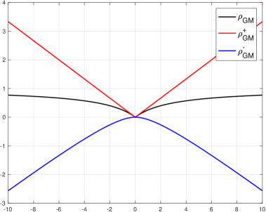
Figure 2: Nonconvexity Redistribution Method for $\rho_{\mathrm{GM}}\left(\left|x\right|\right)$

An illustrating example for Proposition 4 is given in Figure 2. And based on Proposition 4, we can accordingly decompose the row-wise group sparsity regularizer $R\left(\mathbf{B}\right)$ as

$$R\left(\mathbf{B}\right)=R^{+}\left(\mathbf{B}\right)+R^{-}\left(\mathbf{B}\right),$$ (10)

where $R^{+}\left(\mathbf{B}\right)=\kappa\sum_{i=1}^{Q}\xi_{i}\left\|\mathbf{b}_{i}\right\|_{2}$ which exactly takes the form of classical group lasso and $R^{-}\left(\mathbf{B}\right)=R\left(\mathbf{B}\right)-R^{+}\left(\mathbf{B}\right)$. For $R^{-}\left(\mathbf{B}\right)$, we can have the following majorization result.

Lemma 5.

The function $R^{-}\left(\mathbf{B}\right)$ can be majorized at $\mathbf{B}^{\left(k\right)}$ by

$$\overline{R}^{-}\left(\mathbf{B}\right)\simeq\mathrm{Tr}\left(\mathbf{K}^{\left(k\right)T}\mathbf{B}\right),$$

where $\mathbf{K}^{\left(k\right)}=R^{-\prime}\left(\mathbf{B}^{\left(k\right)}\right)$ with $R^{-\prime}\left(\mathbf{B}^{\left(k\right)}\right)$ to be the gradient of $R^{-}\left(\mathbf{B}\right)$ at point $\mathbf{B}^{\left(k\right)}$ and specifically

$$\mathbf{k}_{i}^{\left(k\right)}\triangleq\xi_{i}\left[\rho^{\prime}\left(\left\|\mathbf{b}_{i}^{\left(k\right)}\right\|_{2}\right)-\kappa\right]\frac{\mathbf{b}_{i}^{\left(k\right)}}{\left\|\mathbf{b}_{i}^{\left(k\right)}\right\|_{2}},$$

where $\mathbf{k}_{i}^{\left(k\right)}$ denotes the $i$th column of $\mathbf{K}^{\left(k\right)}$.

Proof:

The proof is trivial and hence omitted. ∎

Based on $\overline{L}\left(\mathbf{B}\right)$ in Lemma 3 and $\overline{R}^{-}\left(\mathbf{B}\right)$ in Lemma 5, we can finally have the majorization function for $F\left(\mathbf{B}\right)$ given as

$$\begin{array}[]{l}\overline{F}\left(\mathbf{B}\right)=\overline{L}\left(\mathbf{B}\right)+R^{+}\left(\mathbf{B}\right)+\overline{R}^{-}\left(\mathbf{B}\right)\\ \quad\quad\quad\simeq\frac{1}{2}\psi\left(\mathbf{G}^{\left(k\right)}\right)\left\|\mathbf{B}-\mathbf{P}_{B,R}^{\left(k\right)}\right\|_{F}^{2}+R^{+}\left(\mathbf{B}\right),\end{array}$$ (11)

where $\mathbf{P}_{B,R}^{\left(k\right)}\triangleq\mathbf{P}_{B}^{\left(k\right)}-\psi^{-1}\left(\mathbf{G}^{\left(k\right)}\right)\mathbf{K}^{\left(k\right)}$. The result by using Lemma 3 and Lemma 5 is that we shift the nonconvexity associated with the nonconvex regularizer to the loss function, and transform the nonconvex regularizer to the familiar convex group lasso regularizer. It is easy to observe that the algorithm derivation above can be easily applied to the classical group lasso and at that case $\mathbf{K}^{\left(k\right)}=\mathbf{0}$.

Finally, the majorizing problem for the $\mathbf{B}$-subproblem is given in the following form:

$$\begin{array}[]{cl}\underset{\mathbf{B}}{\mathsf{minimize}}&\frac{1}{2}\psi\left(\mathbf{G}^{\left(k\right)}\right)\left\|\mathbf{B}-\mathbf{P}_{B,R}^{\left(k\right)}\right\|_{F}^{2}+\frac{1}{\theta}\sum_{i=1}^{Q}\xi_{i}\left\|\mathbf{b}_{i}\right\|_{2}\end{array},$$ (12)

which becomes separable among the rows of matrix $\mathbf{B}$. The resulting separable problems can be efficiently solved using the proximal algorithms [25] and have closed-form solutions which are given in the following lemma.

Lemma 6.

[25] The problem in (12) has a closed-form proximal update which is given by

$$\begin{array}[]{l}\mathbf{b}_{i}^{\left(k+1\right)}=\left[1-\frac{1}{\theta}\frac{\xi_{i}}{\psi\left(\mathbf{G}^{\left(k\right)}\right)}\frac{1}{\left\|\mathbf{p}_{i}^{\left(k\right)}\right\|_{2}}\right]^{+}\mathbf{p}_{i}^{\left(k\right)},\end{array}$$

where $\left[x\right]^{+}\triangleq\max\left(x,0\right)$, and $\mathbf{p}_{i}^{\left(k\right)}$ is the $i$th row of $\mathbf{P}_{B,R}^{\left(k\right)}$.

III-A AltMin-MM: Algorithm for SRRR Estimation

Based on the alternating minimization algorithm together with the majorization and nonconvex redistribution methods, to solve the original SRRR estimation problem (2), we just need to update the variables with closed-form solutions alternatingly until convergence.

The overall algorithm is summarized in the following.

1:$\mathbf{X}$, $\mathbf{Y}$ and $\xi_{i}$ with $i=1,\ldots,r$.

2:Set $k=0$, $\mathbf{A}^{(0)}$ and $\mathbf{B}^{(0)}$.

3:repeat

4:     Compute $\mathbf{P}_{A}^{(k)}$

5:     Update $\mathbf{A}^{\left(k+1\right)}$ in closed-form solution (Lemma 1)

6:     Compute $\mathbf{G}^{(k)}$, $\psi(\mathbf{G}^{(k)})$ and $\mathbf{P}_{B,R}^{(k)}$

7:     Update $\mathbf{B}^{\left(k+1\right)}$ in closed-form solution (Lemma 6)

8:     $k\leftarrow k+1$

9:until convergence

Algorithm 1 AltMin-MM: Algorithm for SRRR Estimation

IV Numerical Simulations

In order to test the performance of the problem model and proposed algorithm. Numerical simulations are considered in this section. An SRRR $\left(P=7,\>Q=5,\>r=3\right)$ with underlying group sparse structure for $\mathbf{B}$ is specified firstly. Then a sample path $\left\{\mathbf{x}_{t},\mathbf{y}_{t},\boldsymbol{\varepsilon}_{t}\right\}_{t=1}^{N}$ is generated.

We first examine the efficiency of our proposed AltMin-MM algorithm when the sparsity regularizer is the group lasso penalty, i.e., $\rho\left(\left|x\right|\right)=\left|x\right|$ which is adopted in [15]. We compare our algorithm with the AltMin-based algorithms with subproblem solved by subgradient method (AltMin-SubGrad) and by variational inequality method (AltMin-VarIneq) for the proposed problem in (2). The convergence result of the objective function value is shown in Fig. 3. It is easy to see that our proposed algorithm can have a faster convergence. It should be mentioned that although the first descent step can attain a better solution in the benchmark methods, since a lot of iterations can be required to get a accuracy enough solution, they show a slower convergence in general.

We further test the case when the regularizer is based on nonconvex Geman function, i.e., $\rho\left(\left|x\right|\right)=\frac{\left|x\right|}{\theta+\left|x\right|}$ ($\theta=0.05$). Since there is no benchmark in the literature, our proposed algorithm AltMin-MM is compared with a benchmark where the convex $\mathbf{B}$-subproblem is derived to be a tight majorized problem of the original problem by just majorizing the nonconvex term $R^{-}\left(\mathbf{B}\right)$ and is solved using $\mathtt{CVX}$. The objective function convergence result is shown in Fig. 3 and Fig. 4.

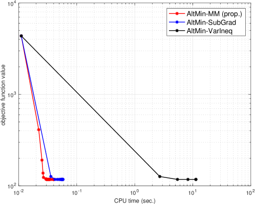
Figure 3: Convergence comparison for objective function value ($N=100$).

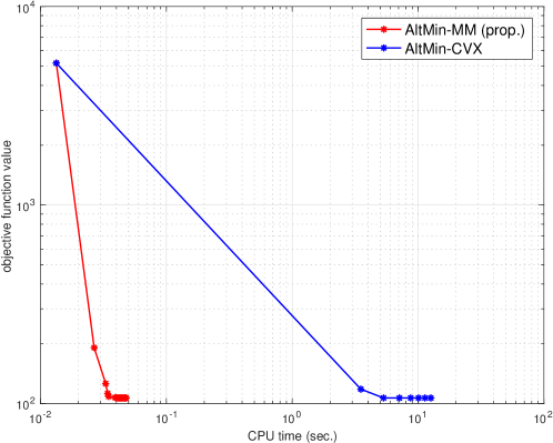
Figure 4: Convergence comparison for objective function value ($N=100$).

We also examine the estimation accuracy of the proposed formulation and algorithm. It is evaluated by computing the angle between the estimated factor matrix space $\hat{\mathbf{B}}^{\left(m\right)}$ and the true space $\mathbf{B}$ denoted by $\theta^{\left(m\right)}(\hat{\mathbf{B}}^{\left(m\right)},\mathbf{B})$ for the $m$th Monte-Carlo simulation, with $m=1,\ldots,M$ and $M=500$. The angle $\theta^{\left(m\right)}(\hat{\mathbf{B}}^{\left(m\right)},\mathbf{B})$ is computed as follows [2]. First, compute the QR decompositions $\hat{\mathbf{B}}^{\left(m\right)}=\mathbf{Q}_{m}\mathbf{R}_{m}$ and $\mathbf{B}=\mathbf{Q}\mathbf{R}$. Next, compute the SVD of $\mathbf{Q}_{m}^{T}\mathbf{Q}=\mathbf{U}_{Q}\mathbf{S}_{Q}\mathbf{V}_{Q}$ where the diagonal elements of $\mathbf{S}_{Q}$ is written as $s_{1}\geq\ldots\geq s_{r}$. Then, the minimum angle is given by $\theta^{\left(m\right)}(\hat{\mathbf{B}}^{\left(m\right)},\mathbf{B})=\arccos\left(s_{1}\right)$. The averaged angle for $M$ Monte-Carlo runs is given by

$$\begin{array}[]{c}\theta(\hat{\mathbf{B}},\mathbf{B})=\frac{1}{M}\sum_{m=1}^{M}\theta^{\left(m\right)}(\hat{\mathbf{B}}^{\left(m\right)},\mathbf{B}),\end{array}$$

where it can take values from $0$ (identical subspaces) to $\frac{\pi}{2}$ (orthogonal subspaces). We compared three cases which are RRR estimation (without sparsity), SRRR estimation with convex sparsity-inducing function $\rho_{\ell_{1}}\left(\left|x\right|\right)$, and SRRR estimation with nonconvex sparsity-inducing function $\rho_{\mathrm{GM}}\left(\left|x\right|\right)$. It is easy to say that, the SRRR problem formulation can really exploit the group sparsity structure in $\mathbf{B}$ and the nonconvex function $\rho_{\mathrm{GM}}\left(\left|x\right|\right)$ shows a better performance over the convex one.

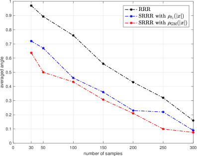
Figure 5: Estimation accuracy based on averaged angle.

V Conclusions

The SRRR model estimation problem has been considered in this paper. It has been formulated to minimize the least squares loss with a group sparsity penalty and considering an orthogonality constraint. A nonconvex nonsmooth sparsity function has been proposed. Efficient algorithm based on the alternating minimization method, the majorization-minimization method and the nonconvexity redistribution method has been developed with variables updated in closed-form. Numerical simulations have shown that the proposed algorithm is more efficient compared to the benchmarks and the nonconvex regularizer can result in a better performance than the convex one.

References

- [1] T. W. Anderson, “Estimating linear restrictions on regression coefficients for multivariate normal distributions,” The Annals of Mathematical Statistics, pp. 327–351, 1951.
- [2] T. W. Anderson, Ed., An Introduction to Multivariate Statistical Analysis. Wiley, 1984.
- [3] A. J. Izenman, “Reduced-rank regression for the multivariate linear model,” Journal of Multivariate Analysis, vol. 5, no. 2, pp. 248–264, 1975.
- [4] M. Viberg, P. Stoica, and B. Ottersten, “Maximum likelihood array processing in spatially correlated noise fields using parameterized signals,” IEEE Transactions on Signal Processing, vol. 45, no. 4, pp. 996–1004, 1997.
- [5] P. Stoica and M. Jansson, “MIMO system identification: State-space and subspace approximations versus transfer function and instrumental variables,” IEEE Transactions on Signal Processing, vol. 48, no. 11, pp. 3087–3099, 2000.
- [6] J. H. Manton and Y. Hua, “Convolutive reduced rank wiener filtering,” in Proc. the 2001 IEEE International Conference on Acoustics, Speech, and Signal Processing (ICASSP’01), vol. 6. IEEE, 2001, pp. 4001–4004.
- [7] E. Lindskog and C. Tidestav, “Reduced rank channel estimation,” in Proc. 1999 IEEE 49th Vehicular Technology Conference,, vol. 2. IEEE, 1999, pp. 1126–1130.
- [8] Y. Hua, M. Nikpour, and P. Stoica, “Optimal reduced-rank estimation and filtering,” IEEE Transactions on Signal Processing, vol. 49, no. 3, pp. 457–469, 2001.
- [9] M. Nicoli and U. Spagnolini, “Reduced-rank channel estimation for time-slotted mobile communication systems,” IEEE Transactions on Signal Processing, vol. 53, no. 3, pp. 926–944, 2005.
- [10] G. Zhou, “Small sample rank tests with applications to asset pricing,” Journal of Empirical Finance, vol. 2, no. 1, pp. 71–93, 1995.
- [11] P. Bekker, P. Dobbelstein, and T. Wansbeek, “The APT model as reduced-rank regression,” Journal of Business & Economic Statistics, vol. 14, no. 2, pp. 199–202, 1996.
- [12] Z. Zhao and D. P. Palomar, “Robust maximum likelihood estimation of sparse vector error correction model,” in Proc. the 2017 5th IEEE Global Conference on Signal and Information Processing, Montreal, QB, Canada, Nov. 2017, pp. 913–917.
- [13] ——, “Mean-reverting portfolio with budget constraint,” IEEE Transactions on Signal Processing, vol. PP, no. 99, p. 1, 2018.
- [14] R. Velu and G. C. Reinsel, Multivariate reduced-rank regression: theory and applications. Springer Science & Business Media, 2013, vol. 136.
- [15] L. Chen and J. Z. Huang, “Sparse reduced-rank regression for simultaneous dimension reduction and variable selection,” Journal of the American Statistical Association, vol. 107, no. 500, pp. 1533–1545, 2012.
- [16] M. Yuan and Y. Lin, “Model selection and estimation in regression with grouped variables,” Journal of the Royal Statistical Society: Series B (Statistical Methodology), vol. 68, no. 1, pp. 49–67, 2006.
- [17] D. P. Bertsekas, Nonlinear programming. Athena scientific Belmont, 1999.
- [18] J. Fan and R. Li, “Variable selection via nonconcave penalized likelihood and its oracle properties,” Journal of the American statistical Association, vol. 96, no. 456, pp. 1348–1360, 2001.
- [19] Y. Sun, P. Babu, and D. P. Palomar, “Majorization-minimization algorithms in signal processing, communications, and machine learning,” IEEE Transactions on Signal Processing, vol. 65, no. 3, pp. 794–816, Aug. 2016.
- [20] Q. Yao and J. T. Kwok, “Efficient learning with nonconvex regularizers by nonconvexity redistribution.” Journal of Machine Learning Research, 2018.
- [21] F. Bach, R. Jenatton, J. Mairal, G. Obozinski et al., “Optimization with sparsity-inducing penalties,” Foundations and Trends® in Machine Learning, vol. 4, no. 1, pp. 1–106, 2012.
- [22] D. Geman and G. Reynolds, “Constrained restoration and the recovery of discontinuities,” IEEE Transactions on Pattern Analysis and Machine Intelligence, vol. 14, no. 3, pp. 367–383, 1992.
- [23] J. C. Gower and G. B. Dijksterhuis, Procrustes problems. Oxford University Press Oxford, 2004, vol. 3.
- [24] M. Hong, M. Razaviyayn, Z.-Q. Luo, and J.-S. Pang, “A unified algorithmic framework for block-structured optimization involving big data: With applications in machine learning and signal processing,” IEEE Signal Processing Magazine, vol. 33, no. 1, pp. 57–77, 2016.
- [25] N. Parikh, S. Boyd et al., “Proximal algorithms,” Foundations and Trends® in Optimization, vol. 1, no. 3, pp. 127–239, 2014.