Supporting Material
Tunable Semiconductors: Control over Carrier States and Excitations in Layered Hybrid Organic-Inorganic Perovskites
Short Description
This Supplemental Material includes: structural details of the perovskites in our simulations; energetic impact of the supercell choice; impact of spin-orbit coupling in the reported energy band structures; computational details (basis sets and k-space grid convergence); validation of computational protocols by comparing to experimental results for MAPbI3, for AE4TPbBr4 and for AE4TPbI4; experimental details for the synthesis and characterization of a new AE4TPbI4 crystal; and additional computed orbitals, energy band structures, band curvature parameters, full and partial densities of states supporting the general findings demonstrated in the actual paper. Computational validation for MAPbI3 also includes comparison to a more sophisticated many-body dispersion treatment.Ambrosetti et al. (2014) Synthesis details include Refs. Muguruma et al. (1996a, b, 1998). All computational input and output files (raw data) are available at the NOMAD repository.NOM
I (22) supercell of AE4TPbBr4
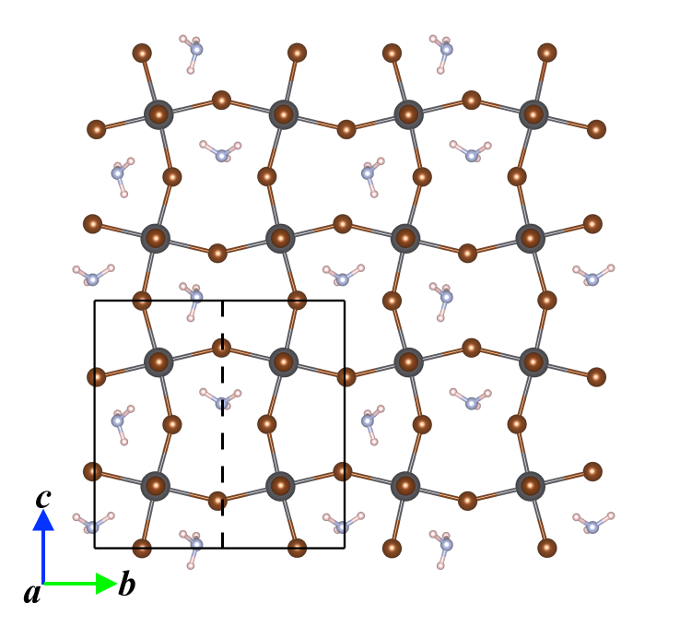
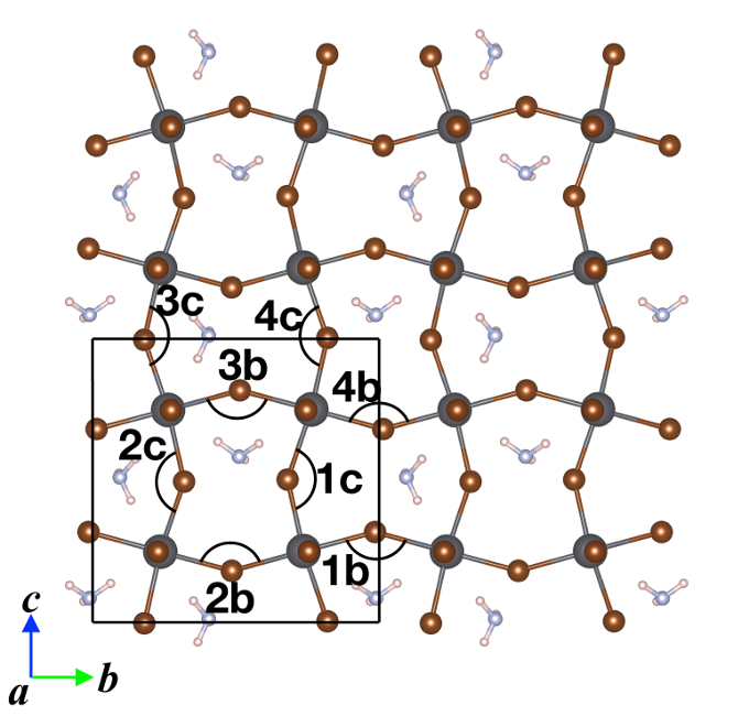
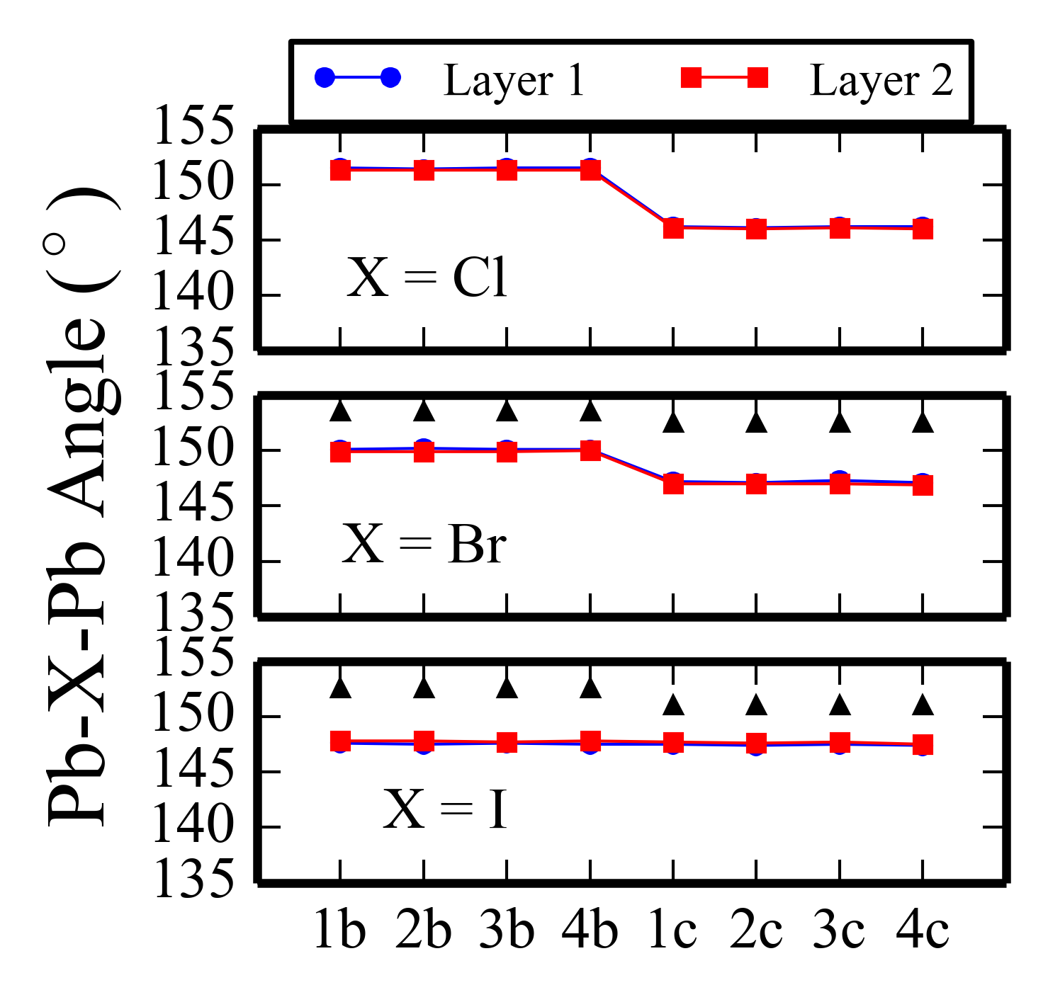
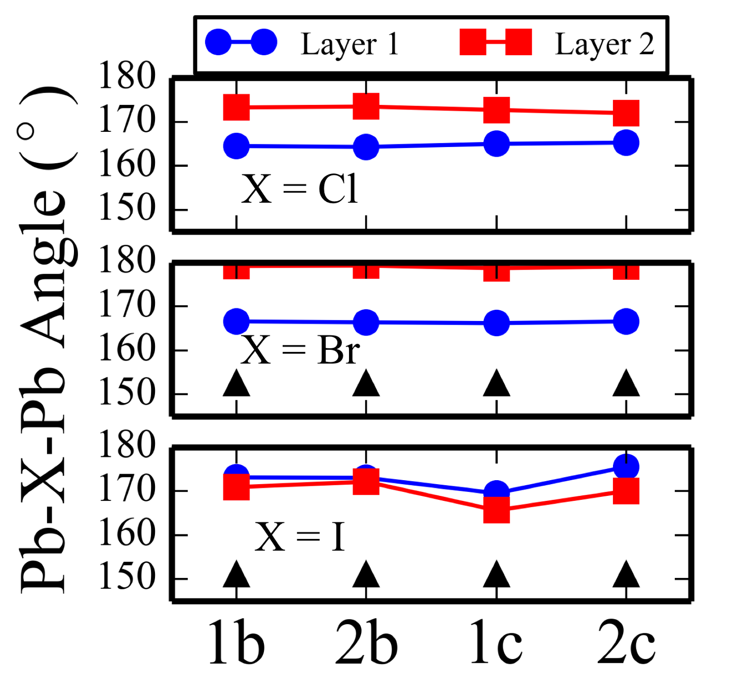
II Comparison of (22) and (12) structure models relaxed by DFT-PBE+TS
II.1 Nomenclature of Pb-X-Pb bond angles (X = Cl, Br, I)
II.2 PBE+TS total energy
| Compounds | Energy Difference (eV) |
|---|---|
| AE4T\cePbCl4 | -2.49 |
| AE4T\cePbBr4 | -2.70 |
| AE4T\cePbI4 | -2.73 |
| AE2T\cePbBr4 | -3.76 |
| AE3T\cePbBr4 | -0.79 |
| all-anti-AE4T\cePbBr4 | -1.50 |
| AE5T\cePbBr4 | -0.83 |
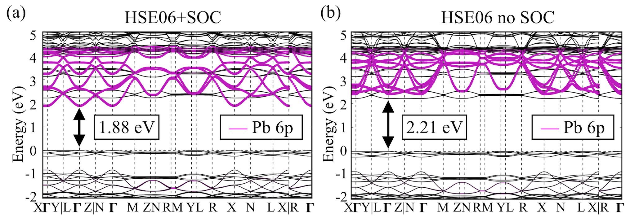
III Effect of spin orbit coupling
IV Computational basis settings: tight
| H | C | N | S | |
| minimal | 1s | [He]+2s2p | [He]+2s2p | [Ne]+3s3p |
| tier 1 | H(2s,2.1) | H(2p,1.7) | H(2p,1.8) | S2+(3d) |
| H(2p,3.5) | H(3d,6.0) | H(3d,6.8) | H(2p,1.8) | |
| H(2s,4.9) | H(3s,5.8) | H(4f,7) | ||
| S2+(3s) | ||||
| tier 2 | H(1s,0.85) | H(4f,9.8) | H(4f,10.8) | H(4d,6.2) |
| H(2p,3.7) | H(3p,5.2) | H(3p,5.8) | H(5g,10.8) | |
| H(2s,1.2) | H(3s,4.3) | H(1s,0.8) | ||
| H(3d,7.0) | H(5g,14.4) | H(5g,16) | ||
| H(3d,6.2) | H(3d,4.9) |
| Cl | Br | I | Pb | |
|---|---|---|---|---|
| minimal | [Ne]+3s3p | [Ar]+4s4p3d | [Kr]+5s5p4d | [Xe]+6s6p5d4f |
| tier 1 | Cl2+(3d) | H(3d,4.6) | H(3d,4) | H(3p,2.3) |
| H(2p,1.9) | H(2p,1.7) | H(4f,6.4) | H(4f,7.6) | |
| H(4f,7.4) | H(4f,7.6) | H(2p,1.6) | H(3d,3.5) | |
| Cl2+(3s) | Br2+(4s) | I2+(5s) | H(5g,9.8) | |
| H(5g,10.4) | H(3s,3.2) | |||
| tier 2 | H(3d,3.3) |
The first line (“minimal”) summarizes the free-atom radial functions used (noble-gas configuration of the core and quantum numbers of the additional valence radial functions). “H(nl, z)” denotes a hydrogen-like basis function for the bare Coulomb potential z/r, including its radial and angular momentum quantum numbers, n and l. X2+(nl) denotes a n, l radial function of a doubly positive free ion of species X. This nomenclature follows the convention employed in Table 1 of Ref. Blum et al. (2009).
V K-grid convergence test
| K-grid | (eV) | (meV/atom) |
|---|---|---|
| 122 | 0* | 0* |
| 244 | -0.066 | -0.16 |
* reference value
VI Computational basis settings: intermediate
| H | C | N | S | |
| minimal | 1s | [He]+2s2p | [He]+2s2p | [Ne]+3s3p |
| tier 1 | H(2s,2.1) | H(2p,1.7) | H(2p,1.8) | S2+(3d) |
| H(2p,3.5) | H(3d,6.0) | H(3d,6.8) | H(2p,1.8) | |
| H(2s,4.9) | H(3s,5.8) | H(4f,7) | ||
| S2+(3s) | ||||
| tier 2 | H(1s,0.85) | H(4f ,9.8) | H(4f,10.8) | H(5g,10.8)aux |
| H(3d,7.0)aux | H(5g,14.4)aux | H(5g,16)aux |
| Cl | Br | I | Pb | |
| Minimal | [Ne]+3s3p | [Ar]+4s4p3d | [Kr]+5s5p4d | [Xe]+6s6p5d4f |
| tier 1 | Cl2+(3d) | H(3d,4.6) | H(3d,4) | H(3p,2.3) |
| H(2p,1.9) | H(2p,1.7) | H(4f,6.4) | H(4f,7.6) | |
| H(4f,7.4) | H(4f,7.6) | H(2p,1.6) | H(3d,3.5) | |
| Cl2+(3s) | Br2+(4s) | I2+(5s) | H(5g,9.8)aux | |
| H(5g,10.4) | H(3s,3.2) | |||
| tier 2 | H(3d,3.3) | |||
| H(5g,10.8)aux | H(5g,10.4)aux | H(5g,9.4)aux |
The first line (“minimal”) summarizes the free-atom radial functions used (noble-gas configuration of the core and quantum numbers of the additional valence radial functions). “H(nl, z)” denotes a hydrogen-like basis function for the bare Coulomb potential z/r, including its radial and angular momentum quantum numbers, n and l. X2+(nl) denotes a n, l radial function of a doubly positive free ion of species X. This nomenclature follows the convention employed in Table 1 of Ref. Blum et al. (2009). The subscript “aux” denotes a basis function that is not used to expand the actual, generalized Kohn-Sham orbitals but that is used during the creation of the auxiliary basis sets that expand the screened Coulomb operator of the HSE06 functional, following the method described in Ref. Ihrig et al. (2015).
VII Validation of the computational approach
(a)
(b)
Lattice parameters (Å)
Source
a
b
c
Volume (Å3)
Eg (eV)
Exp. Weller et al. (2015)
8.8657
12.6293
8.5769
960.3
1.65-1.675 Kong et al. (2015)
1.68 Phuong et al. (2016)
PBE
9.25
12.88
8.62
1027
1.42 (HSE06+SOC)
deviation
4.3 %
2.0 %
0.5 %
7.0 %
PBE+TS
8.99
12.71
8.48
968.1
1.42 (HSE06+SOC)
deviation
1.4 %
0.6 %
1.1 %
0.8 %
PBE+MBD
9.00
12.72
8.48
971
1.43 (HSE06+SOC)
deviation
1.5 %
0.7 %
1.2 %
1.1 %
VIII Optimized structures of AE4TPbX4 (X = Cl, Br, I)
| HOIPs | a(Å) | b(Å) | c(Å) | V(Å3) | |||
| AE4T\cePbCl4 | |||||||
| PBE+TS | 40.85 | 11.29 | 10.95 | 90.0∘ | 91.8∘ | 90.0∘ | 5049 |
| AE4T\cePbBr4 | |||||||
| Exp.Mitzi et al. (1999) | 39.74 | 11.68 | 11.57 | 90.0∘ | 92.4∘ | 90.0∘ | 5369 |
| PBE+TS | 40.01 | 11.60 | 11.47 | 90.0∘ | 91.3∘ | 90.0∘ | 5322 |
| (%) | 0.67 | -0.74 | -0.87 | 0.02 | -1.17 | 0.04 | -0.88 |
| AE4T\cePbI4 | |||||||
| Exp.∗ | 38.79 | 12.18 | 12.33 | 90.0∘ | 92.3∘ | 90.0∘ | 5818 |
| PBE+TS | 39.02 | 12.10 | 12.22 | 90.0∘ | 91.1∘ | 90.0∘ | 5771 |
| (%) | 0.59 | -0.65 | -0.86 | 0.04 | -1.31 | 0.04 | -0.81 |
* see Section S8, “Experimental details for AE4T\cePbI4”, in this work.
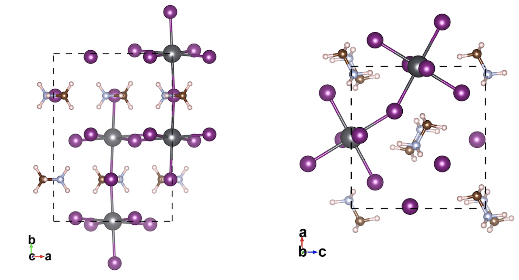
IX Construction of the computational structure models of the HOIP compounds assessed in this work
We perform full relaxation of both unit cell parameters and cell-internal atomic coordinates on the initial input structure for all the HOIPs investigated. Initial models for the structure optimization were constructed as follows:
-
•
AE4T\cePbBr4: Taken as the experimental structure in Ref. Mitzi et al. (1999).
-
•
AE4T\cePbX4 (X = Cl, I): Obtained by taking the experimental structure of AE4T\cePbBr4 and replacing the Br atoms with Cl and I. The lattice parameters and the atomic coordinates of non-halogen atoms were kept the same among the three hybrid compounds for the input structure. The initial configuration of AE4T molecules was kept to be syn-anti-syn as in the experimental structure of AE4T\cePbBr4.
-
•
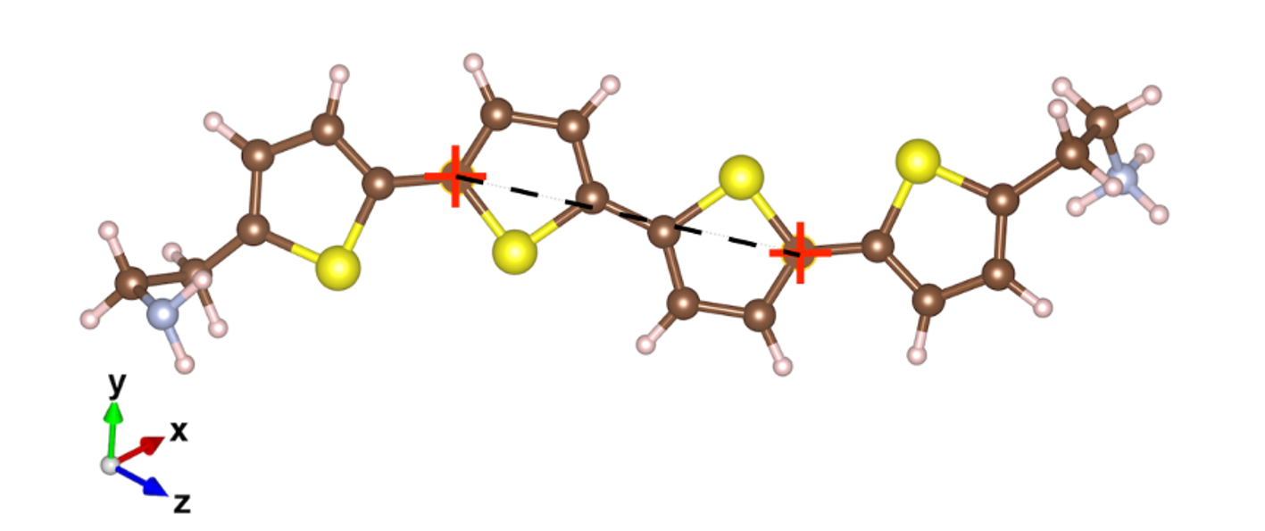
all-anti-AE4T\cePbBr4: Obtained by taking the experimental structure of AE4T\cePbBr4 and changing the configuration of AE4T to all-anti. The inner two thiophene rings of the syn-anti-syn AE4T were rotated by 180∘ around the two C atoms labeled by red “+” as the rotation axis (Fig. S7). This rotation was performed for all the 8 AE4T molecules in the unit cell.
-
•
AEnT\cePbBr4 (n = 1, 2, 3, 5): Obtained by taking the experimental structure of AE4T\cePbBr4 and replacing the AE4T organic part by all-anti AEnT molecules. Using AE3T-\cePbBr4 as an example, we start from the experimental structure of AE4T\cePbBr4 with syn-anti-syn AE4T molecules. The oligothiophene part (4T) is removed while the inorganic Pb-Br framework together with the \ceEtNH3 tails are kept–i.e., the configuration of the Pb-Br framework together with the \ceEtNH3 tails is not changed during the construction. The adjacent inorganic layers are then pushed towards each other to reduce the distance between them to the extent that it is suitable for the insertion of the 3T molecules (all-anti). We then place the optimized 3T molecules into those positions where the 4T molecules originally existed (for AE4T\cePbBr4). This construction process preserves the configuration between the inorganic Pb-Br framework and the \ceEtNH3 tails (Fig. S1) and keeps the two inorganic layers in each unit cell identical.
X Experimental details for AE4T\cePbI4
Chemical. \cePbI2 (99.999% trace metal basis), HI (57 wt. % in \ceH2O, with hypophosphorous acid as stabilizer, assay 99.95%) and N,N-Dimethylformamide (anhydrous, 99.8%) were purchased from Sigma-Aldrich company. AE4THI was synthesized in the lab.Muguruma et al. (1996a, b, 1998) 2-butanol (99.5%) was purchased from VWR International.
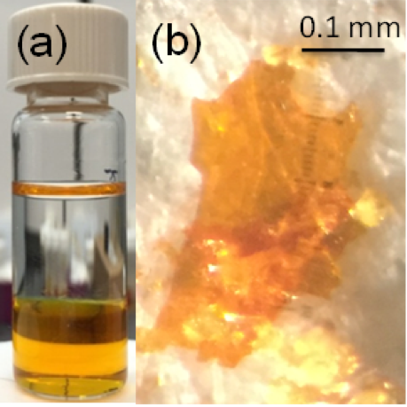
Synthesis. 2 mg \cePbI2 and 3 mg AE4THI were dissolved in 0.7 ml DMF with a drop of HI. Then, 2 ml 2-butanol was layered on the top of the solution (Figure S8a). The target crystals came out after several days (Figure S8b).
Characterization. Single crystal X-ray diffraction data were collected in a Bruker D8 ADVANCE Series II at room temperature. The unit cell parameters determined from this data are a = 38.779(3) Å, b = 6.0863(5) Å, c = 12.3306(10) Å, = 92.271(4), V = 2908.0(4) Å3, C2/c.
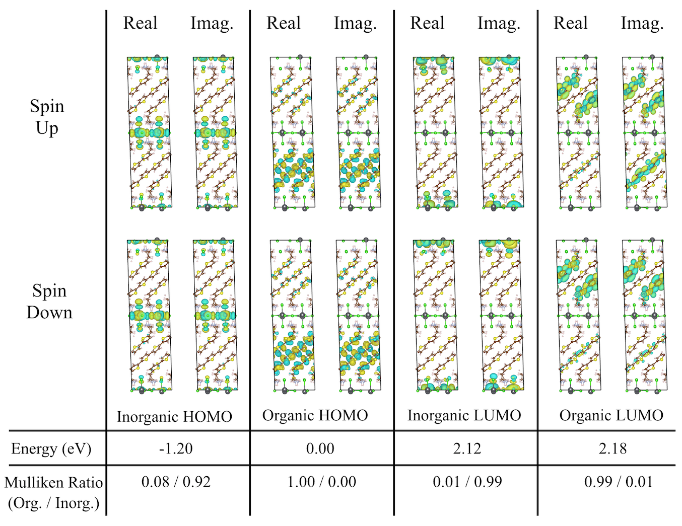
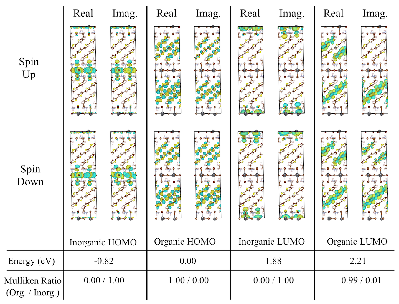
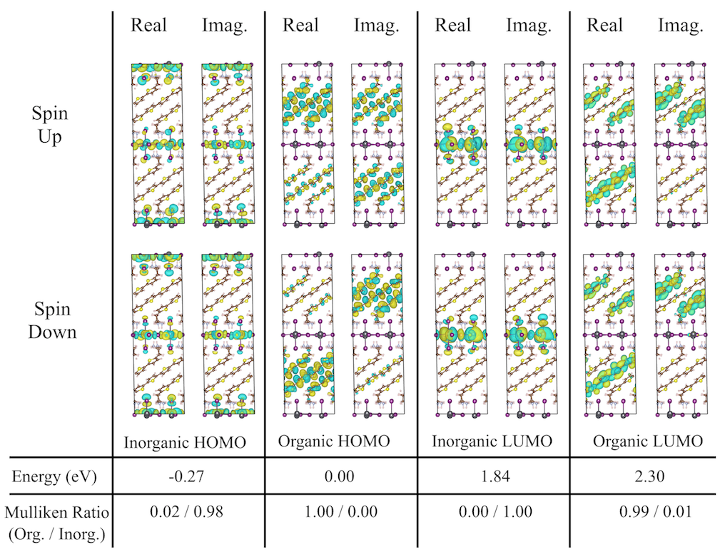
XI DFT-HSE06+SOC frontier orbitals for AE4TPbX4 (X=Cl, Br, I)
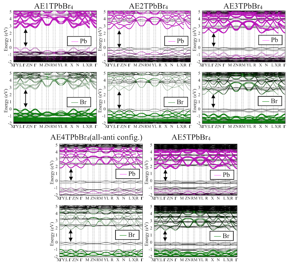
XII DFT-HSE06+SOC band structures of AEnTPbBr4 (n = 1, 2, 3, 4, 5)
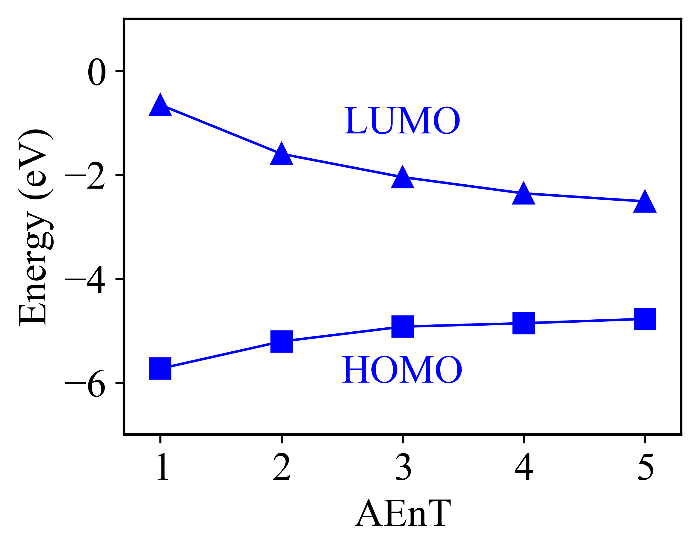
XIII HOMO-LUMO Gaps of isolated oligothiophene molecules
XIV Effective Mass Parameters Derived from the Band Structures Computed in This Work
| Material | Direction | HOMO (inorg.) | HOMO (org.) | LUMO (inorg.) | LUMO (org.) |
|---|---|---|---|---|---|
| AE4TPbCl4 | -X | 20 | 20∗ | 20∗ | 20 |
| -Y | 0.42 | 20∗ | 0.32∗ | 1.38 | |
| -Z | 0.46 | 2.66∗ | 0.43∗ | 6.8 | |
| AE4TPbBr4 | -X | 20 | 20∗ | 20∗ | 20 |
| -Y | 0.31 | 20∗ | 0.26∗ | 1.57 | |
| -Z | 0.33 | 2.23∗ | 0.31∗ | 15.9 | |
| AE4TPbI4 | -X | 17.3 | 20∗ | 20∗ | 20 |
| -Y | 0.27 | 20∗ | 0.22∗ | 7.6 | |
| -Z | 0.27 | 11.4∗ | 0.22∗ | 9.0 |
| Material | Direction | HOMO (inorg.) | HOMO (org.) | LUMO (inorg.) | LUMO (org.) |
|---|---|---|---|---|---|
| AE1TPbBr4 | -X | 11.1∗ | 5.1 | 20∗ | 20 |
| -Y | 0.37∗ | 4.6 | 0.23∗ | 0.97 | |
| -Z | 0.38∗ | 1.7 | 0.44∗ | 1.08 | |
| AE2TPbBr4 | -X | 20 | 20∗ | 20∗ | 6.9 |
| -Y | 0.33 | 7.5∗ | 0.23∗ | 16.9 | |
| -Z | 0.37 | 1.2∗ | 0.36∗ | 2.9 | |
| AE3TPbBr4 | -X | 20 | 20∗ | 20∗ | 20 |
| -Y | 0.38 | 20∗ | 0.24∗ | 2.8 | |
| -Z | 0.39 | 1.9∗ | 0.55∗ | 20 | |
| AE4TPbBr4 (all-anti) | -X | 16.3 | 20∗ | 20∗ | 20 |
| -Y | 0.40 | 5.6∗ | 0.24∗ | 2.3 | |
| -Z | 0.39 | 1.1∗ | 0.35∗ | 20 | |
| AE5TPbBr4 | -X | 20 | 20∗ | 20∗ | 20 |
| -Y | 0.55 | 7.3∗ | 0.24∗ | 5.5 | |
| -Z | 0.54 | 1.2∗ | 0.55∗ | 2.8 |
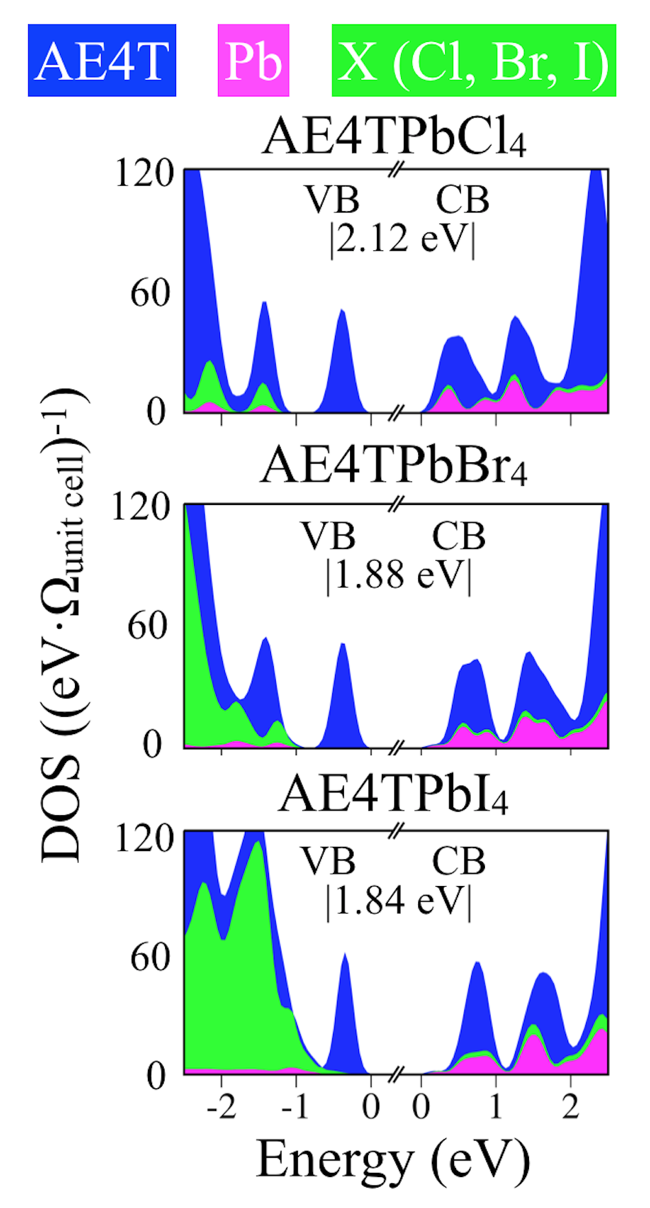
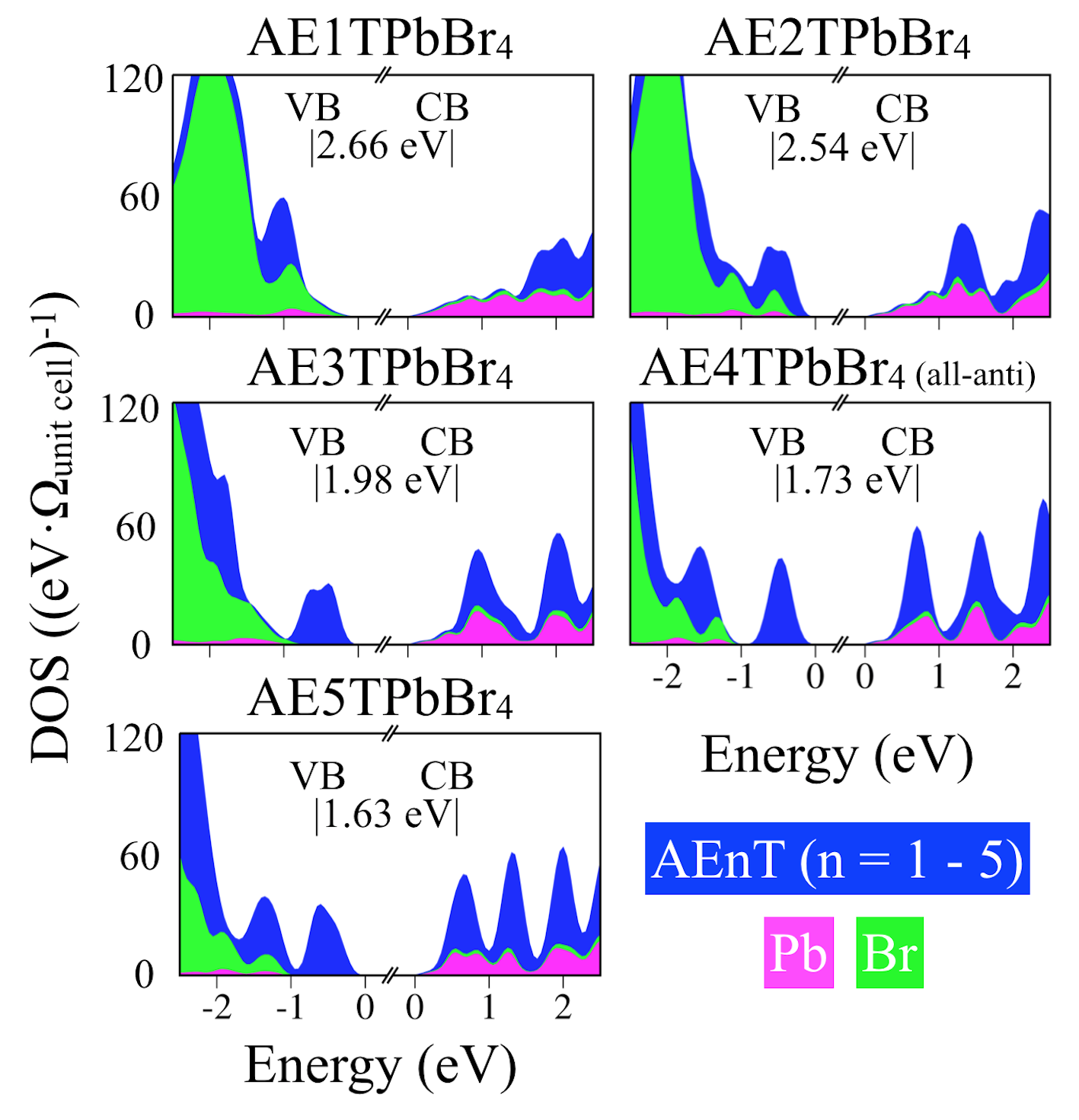
XV Total and Partial Densities of States
References
- Ambrosetti et al. (2014) A. Ambrosetti, A. M. Reilly, R. A. DiStasio Jr., and A. Tkatchenko, J. Chem. Phys. 140, 18A508 (2014).
- Muguruma et al. (1996a) H. Muguruma, T. Saito, A. Hiratsuka, I. Karube, and S. Hotta, Langmuir 12, 5451 (1996a).
- Muguruma et al. (1996b) H. Muguruma, T. Saito, S. Sasaki, S. Hotta, and I. Karube, J. Heterocyclic Chem. 33, 173 (1996b).
- Muguruma et al. (1998) H. Muguruma, K. Kobiro, and S. Hotta, Chem. Mater. 10, 1459 (1998).
- (5) NOMAD Repository. http://doi.org/10.17172/NOMAD/2018.09.21-1 (accessed Sep 22, 2018).
- Mitzi et al. (1999) D. B. Mitzi, K. Chondroudis, and C. R. Kagan, Inorg. Chem. 38, 6246 (1999).
- Blum et al. (2009) V. Blum, R. Gehrke, F. Hanke, P. Havu, V. Havu, X. Ren, K. Reuter, and M. Scheffler, Comput. Phys. Commun. 180, 2175 (2009).
- Ihrig et al. (2015) A. C. Ihrig, J. Wieferink, I. Y. Zhang, M. Ropo, X. Ren, P. Rinke, M. Scheffler, and V. Blum, New Journal of Physics 17, 093020 (2015).
- Weller et al. (2015) M. T. Weller, O. J. Weber, P. F. Henry, A. M. Di Pumpo, and T. C. Hansen, Chem. Commun. 51, 4180 (2015).
- Kong et al. (2015) W. Kong, Z. Ye, Z. Qi, B. Zhang, M. Wang, A. Rahimi-Iman, and H. Wu, Phys. Chem. Chem. Phys. 17, 16405 (2015).
- Phuong et al. (2016) L. Q. Phuong, Y. Yamada, M. Nagai, N. Maruyama, A. Wakamiya, and Y. Kanemitsu, J. Phys. Chem. Lett. 7, 2316 (2016).
- Perdew et al. (1996) J. P. Perdew, K. Burke, and M. Ernzerhof, Phys. Rev. Lett. 77, 3865 (1996).
- Tkatchenko and Scheffler (2009) A. Tkatchenko and M. Scheffler, Phys. Rev. Lett. 102, 073005 (2009).