Probing the Production of Extreme-ultraviolet Late-Phase Solar Flares by Using the Model Enthalpy-Based Thermal Evolution of Loops

Abstract

Recent observations in extreme-ultraviolet (EUV) wavelengths reveal an EUV late phase in some solar flares that is characterized by a second peak in warm coronal emissions ($\sim 3$ MK) several tens of minutes to a few hours after the soft X-ray (SXR) peak. Using the model enthalpy-based thermal evolution of loops (EBTEL), in this paper we numerically probe the production of EUV late-phase solar flares. Starting from two main mechanisms of producing the EUV late phase, i.e., long-lasting cooling and secondary heating, we carry out two groups of numerical experiments to study the effects of these two processes on the emission characteristics in late-phase loops. In either of the two processes an EUV late-phase solar flare that conforms to the observational criteria can be numerically synthesized. However, the underlying hydrodynamic and thermodynamic evolutions in late-phase loops are different between the two synthetic flare cases. The late-phase peak due to a long-lasting cooling process always occurs during the radiative cooling phase, while that powered by a secondary heating is more likely to take place in the conductive cooling phase. We then propose a new method for diagnosing the two mechanisms based on the shape of EUV late-phase light curves. Moreover, from the partition of energy input, we discuss why most solar flares are not EUV late flares. Finally, by addressing some other factors that may potentially affect the loop emissions, we also discuss why the EUV late phase is mainly observed in warm coronal emissions.

1 INTRODUCTION

It is widely accepted that solar flares are a result of the rapid release of magnetic energy stored in the solar corona. Through the magnetic reconnection process (Parker, 1963), the free magnetic energy is rapidly converted into plasma heating in the flare loops, acceleration of charged particles, and in some cases, bulk plasma motion, which is later on manifested as a coronal mass ejection (CME) propagating into the interplanetary space.

When the impulsive flare heating is terminated, the flare loops will naturally cool down. This cooling process, however, is far from a static. Powered by an intense flare heating, the flare loop can initially be heated to a temperature as high as several tens of megakelvin. This builds up a huge temperature gradient along the loop, resulting in a large heat flux conducting down into the transition region (TR) and chromosphere during the early cooling stage. In addition to the bombardment by a nonthermal electron beam, this excess heat flux must also drive an upward flow from the TR/chromosphere (Neupert, 1968), which is conventionally termed chromospheric evaporation (Antiochos & Sturrock, 1978), otherwise the heat flux would be too high to be effectively radiated away in the TR/chromosphere (Antiochos & Sturrock, 1976). As the loop temperature decreases and the density increases, radiation gradually becomes dominant. In a loop under radiative cooling, regions of lower temperatures cool faster than those of higher temperatures (Antiochos, 1980), as expected from the shape of the radiative loss function. This difference in cooling rate weakens the pressure gradient along the loop that balances against gravity, which, except for a static catastrophic cooling in the very late stage (Cargill & Bradshaw, 2013), consequently leads to a downward flow into the TR/chromosphere (Bradshaw & Cargill, 2005), usually known as chromospheric condensation.

Observationally, the evolution of temperature and density in flare loops can be quantitatively diagnosed via the electromagnetic emissions from the loops in a wide wavelength range. According to the standard two-ribbon solar flare model, which is often called the CSHKP model (Carmichael, 1964; Sturrock, 1966; Hirayama, 1974; Kopp & Pneuman, 1976), the evolution of a solar flare can be divided into two phases: an impulsive phase, and a following gradual phase. The impulsive phase is characterized by a rapid increase of the emissions in hard X-ray (HXR) and chromospheric lines (e.g., He II), indicating a prompt response of the solar lower atmosphere to the nonthermal electron bombardment and/or thermal conduction caused by the initial heating. Hot evaporated material then fills the flare loops, which brighten up in soft X-ray (SXR) and coronal lines. In particular, the loop emissions peak in extreme-ultraviolet (EUV) wavelengths in the sequence of decreasing temperatures, constituting the gradual phase (Chamberlin et al., 2012).

In general, during the gradual phase of a solar flare, the EUV emission exhibits just one main peak shortly after the GOES SXR peak. Nevertheless, by using full-disk integrated EUV irradiance observations with the EUV Variability Experiment (EVE; Woods et al., 2012) on board the Solar Dynamics Observatory (SDO; Pesnell et al., 2012), Woods et al. (2011) discovered an “EUV late phase” in some flares, which is seen as a second peak in the warm coronal emissions (e.g., Fe XVI, $\sim 3$ MK) several tens of minutes to a few hours after the GOES SXR peak. There are, however, no significant enhancements of the SXR or hot coronal emissions (e.g., Fe XX and higher, $>10$ MK) in the EUV late phase, and spatially resolved imaging observations such as from the Atmospheric Imaging Assembly (AIA; Lemen et al., 2012) on board the SDO reveal that the secondary late-phase emission comes from a set of higher and longer loops that are anchored in the same flare-hosting active region (AR) as the original flaring loops.

In a statistics of 191 solar flares higher than the GOES C2 class that occurred during the first year of SDO normal operations, Woods et al. (2011) found that only 25 of them (13%) exhibited an EUV late phase, and more interestingly, about half of the EUV late-phase flares took place in a cluster of two ARs, implying a specific magnetic configuration of the ARs in which EUV late-phase flares are preferentially produced. Case studies showed that EUV late-phase flares occur in a multipolar magnetic field, which exhibits either a classic or asymmetric quadrupolar configuration (Hock et al., 2012; Liu et al., 2013a), or a parasitic polarity embedded in a large-scale bipolar magnetic field (Dai et al., 2013; Sun et al., 2013; Masson et al., 2017). Such a magnetic configuration observationally facilitates the existence of two sets of loops that are distinct in length rather than loops with a continuous length distribution, as further confirmed by force-free coronal magnetic field extrapolations (Jiang et al., 2013; Sun et al., 2013; Li et al., 2014a; Guo et al., 2017; Masson et al., 2017).

The discovery of the EUV late phase imposed a great challenge to current empirical flare-irradiance models (e.g., Tobiska et al., 2000; Chamberlin et al., 2008), since they use the emission measured in SXRs as a flare proxy, and therefore would improperly estimate the total flare energy if there exists an EUV late phase in the flare. However, currently, only a few reports on the EUV late phase are available in the literature, and the origin of this phase is still not fully understood. Based on the observational facts mentioned above, some authors suggested that the EUV late phase might be due to a secondary energy injection into the long late-phase loops that is considerably delayed from the main flare heating (Woods et al., 2011; Hock et al., 2012; Dai et al., 2013), while others proposed that both the main flaring loops and late-phase loops are heated nearly simultaneously during the main flare heating, and the delayed occurrence of the EUV late phase is the result of a long-lasting cooling process in the long-late phase loops (Liu et al., 2013a; Masson et al., 2017). It was also pointed out that in some EUV late-phase flares the two mechanisms may both play a role (Sun et al., 2013).

Through numerical experiments using the model called enthalpy-based thermal evolution of loops (EBTEL), which was first proposed by Klimchuk et al. (2008) and later improved by Cargill et al. (2012a) and Barnes et al. (2016), Li et al. (2014a) numerically studied the role of the above two mechanisms in producing an EUV late phase, finding that a long cooling process in the late-phase loops can well explain the presence of the EUV late-phase emission, although the possibility of an additional heating in the decay phase cannot be excluded. Nevertheless, until now the EUV late-phase emission characteristics under different mechanisms have not been studied in depth to date, but deserve further investigation. As a time-efficient model, the EBTEL model is very suitable for such studies. Using the EBTEL model, we here explore the physical relationship between the emission characteristics and the underlying hydrodynamics and thermodynamics in different flare loops, and try to answer the important questions why EUV late-phase flares only occupy a small fraction in all solar flares and why the EUV late phase is mainly observed in warm coronal emissions. The paper is organized as follows. In Section 2 we briefly describe the EBTEL model. In Section 3 we carry out two groups of numerical experiments, and use the outputs to synthesize different EUV late-phase flares. The numerical results are discussed in detail in Section 4, and a brief summary is presented in Section 5.

2 The EBTEL MODEL

The EBTEL model is a zero-dimensional (0D) hydrodynamic model that describes the evolution of the average temperature, pressure, and density along a coronal loop. When compared with those far more sophisticated one-dimensional (1D) hydrodynamic numerical simulations, EBTEL gives quite good agreement in average parameters, but is costs far less computation time.

The basic idea behind EBTEL is that the imbalance between the heat flux conducting down into the TR and the radiative loss rate there leads to an enthalpy flux at the coronal base: an excess heat flux drives an evaporative upflow, whereas a deficient heat flux is compensated for by a condensation downflow. This upward/downward enthalpy flow controls the hydrodynamic evolution of the coronal loop. We note that this idea has also been adopted to treat the “unresolved TR” in the recent 1D modeling in Johnston et al. (2017).

If the flows along the loop are subsonic (which should hold for the most of the time of the evolution), the kinetic energy can be neglected and the equation of momentum can be dropped from the governing equations. By integrating the equations of continuity and energy conservation over the coronal section of the loop, which has a half-length $L$ measured from the coronal base to apex (EBTEL assumes a symmetric semi-circular loop geometry), we obtain

$$\frac{dn}{dt}=-\frac{c_{2}}{5c_{3}kTL}(F_{0}+c_{1}\mathcal{R}_{c})$$ (1)

and

$$\frac{dp}{dt}=\frac{2}{3}\left[Q-(1+c_{1})\frac{\mathcal{R}_{c}}{L}\right],$$ (2)

where $n$, $p$, and $T$ are the average density, pressure, and temperature of the coronal loop, respectively, $k$ is the Boltzmann constant, $c_{2}$ ($c_{3}$) is the ratio of the average coronal (coronal base) temperature to apex temperature, $F_{0}=-(2/7)\kappa_{0}(T/c_{2})^{7/2}/L$ (where $\kappa_{0}=8.12\times 10^{-7}$ in cgs units is the classical Spitzer thermal conduction coefficient) is the heat flux at the coronal base, $\mathcal{R}_{c}={n}^{2}\Lambda(T)L$ (where $\Lambda(T)$ is the optically thin radiative loss function) approximates the radiative loss rate from the corona, $c_{1}$ is the ratio of radiative loss rate of the TR to that of the corona, and $Q$ is the average volumetric heating rate. For brevity, we omit the word “average”: so if not explicitly specified, hereafter quantities like density, pressure, temperature, and heating rate refer to the loop-averaged quantities. The evolution of the coronal temperature then follows from the equation of state, which is

$$\frac{1}{T}\frac{dT}{dt}=\frac{1}{p}\frac{dp}{dt}-\frac{1}{n}\frac{dn}{dt}.$$ (3)

Of the three parameters $c_{1}$, $c_{2}$, and $c_{3}$ in EBTEL, $c_{1}$ is the most important. Analytical calculations based on the static coronal loop model in Martens (2010) gave a value for $c_{1}$ of around 2, and values for $c_{2}$ and $c_{3}$ close to 0.9 and 0.6, respectively. In the original EBTEL model (Klimchuk et al., 2008), to achieve an overall consistency with the 1D simulation results, $c_{1}$ was kept as a constant of 4 throughout the loop evolution. Nevertheless, when a loop evolves dynamically, the equilibrium is broken and $c_{1}$ will also evolve. Obviously, the choice of a fixed $c_{1}$ value is not physically reasonable. In the later EBTEL versions, more physics was included to more appropriately determine the values of $c_{1}$. One piece of the physics previously absent is gravitational stratification, whose main effect is to depress the coronal radiation. Thus, higher values of $c_{1}$ can be expected, especially for long loops with significant ratios of the length to the gravitational scale height (Cargill et al., 2012a). Another one piece is the deviation of the dynamically cooling loop from equilibrium states. In the early conductive cooling phase, the density increase in response to the strong heat flux is not so fast that the loop is under-dense with respect to a static loop at the same temperature, leading to higher values of $c_{1}$ (Barnes et al., 2016). During the radiative cooling phase, the loop is instead overdense, which will in turn reduce the $c_{1}$ values (Cargill et al., 2012a). In our following numerical experiments, we consistently calculate $c_{1}$ by taking all these factors into account, and hold $c_{2}$ and $c_{3}$ at their typical values of 0.9 and 0.6, respectively.

3 NUMERICAL EXPERIMENTS

We use EBTEL to trace the hydrodynamic response of coronal loops to an impulsive energy release. For a prescribed loop half-length $L$ and volumetric heating rate function $Q(t)$, we obtain the temporal evolution of the temperature $T(t)$, density $n(t)$, and pressure $p(t)$ of a coronal loop by numerically solving the time-dependent EBTEL Equations (1)–(3). Then we use the outputs to synthesize the EUV emissions of the loop as they are in real solar observations. The overall light curves of a solar flare can be synthetically generated by combining the emissions of a series of loops with different lengths and/or energy injections. We have carried out two groups of numerical experiments to probe the effects of varying the prescribed parameters on the loop emission characteristics and their implications in the production of an EUV late-phase flare.

3.1 Experiment 1: Effect of the Loop Length

Previous case studies of EUV late phase flares showed that the EUV late-phase emission originates from a second set of higher and longer loops (Hock et al., 2012; Dai et al., 2013; Liu et al., 2013a, 2015; Sun et al., 2013; Masson et al., 2017). The long-lasting cooling process explanation suggests that the EUV late-phase loops are heated nearly simultaneously with the main flaring loops, and their delay in warm EUV emissions is attributed to a longer cooling process for greater loop lengths (Liu et al., 2013a; Li et al., 2014a; Masson et al., 2017). In EBTEL numerical experiment 1, we therefore vary the loop half-length and check its influence on the emission properties of the loops.

Table 1: Parameters in the EBTEL Numerical Experiments

No.	$L$	$A_{\mathrm{pix}}$	$Q_{0}$	$\tau_{H}$	$Q_{b}$	$T(t=0)$	$n(t=0)$
	($10^{9}$ cm)	(AIA pixel)	(erg cm-3 s-1)	(s)	(erg cm-3 s-1)	(MK)	(108 cm-3)
Experiment 1
$i=1$ (M1)	1.5	1	1.500	300	$10^{-5}$	0.44	0.86
$i=2$	3.0	1	0.750	300	$10^{-5}$	0.66	0.89
$i=3$	4.5	1	0.500	300	$10^{-5}$	0.83	0.90
$i=4$	6.0	1	0.375	300	$10^{-5}$	0.97	0.89
$i=5$ (L1)	7.5	1	0.300	300	$10^{-5}$	1.11	0.89
$i=6$	9.0	1	0.250	300	$10^{-5}$	1.23	0.88
$i=7$	10.5	1	0.214	300	$10^{-5}$	1.34	0.87
$i=8$	12.0	1	0.188	300	$10^{-5}$	1.45	0.86
$i=9$	13.5	1	0.167	300	$10^{-5}$	1.56	0.86
$i=10$	15.0	1	0.150	300	$10^{-5}$	1.66	0.86
Experiment 2
$i=1$ (L1)	$7.5$	1	$0.300$	300	$10^{-5}$	1.11	0.89
$i=2\cdots 4$	$7.5$	$10^{(i-1)/2}$	$3\times 10^{-(i+1)/2}$	300	$10^{-5}$	1.11	0.89
$i=5$ (L2)	$7.5$	$100$	$0.003$	300	$10^{-5}$	1.11	0.89

Note. — The columns show the loop half-length (Column 2), normalized loop cross-sectional area (Column 3), peak rate of the triangular heating pulse (Column 4), duration of the pulse (Column 5), background heating rate (Column 6), initial loop temperature (Column 7), and density (Column 8).

The parameters in experiment 1 are listed in the upper rows of Table 1. Here we consider a total of 10 loops, whose half-lengths consecutively increase from $1.5\times 10^{9}$ cm to $1.5\times 10^{10}$ cm with an even step of $1.5\times 10^{9}$ cm. Note that the specification of $L$ values is not arbitrary but based on observations. Loops lying toward the short end of our loop cases have lengths typical of main flaring loops, whereas those considerably longer (length ratio $>$ 2) correspond to late-phase loops (Dai et al., 2013; Liu et al., 2013a; Sun et al., 2013). The initial equilibria in the loops are maintained by a steady background heating with a heating rate $Q_{b}$ of $10^{-5}$ erg cm^-3 s^-1. As shown in the last two columns of Table 1, the initial loop density is almost a constant close to $9\times 10^{7}$ cm^-3 in the different loops, while the initial temperature increases monotonically from 0.44 MK to 1.66 MK as the loop half-length increases. This temperature increase tendency can be mathematically expected from the general equilibrium solutions of EBTEL, which reveal a scaling relationship as $T\sim L^{4/7}$. Generally speaking, if a short loop were initially heated to the same temperature as in a longer static loop, a too large temperature gradient would be built up along the short loop, with the resulting excess heat flux in turn quickly smoothing this sharp temperature gradient.

Starting from the initial equilibria, we impose an impulsive heating on the loops, whose heating rate $Q$ has a triangular profile with a total duration $\tau_{H}$ of 300 s (with equal ascending and descending durations), comparable to the duration of the impulsive phase in a typical solar flare. The peak values $Q_{0}$ of the heating rate are set in such a way that for the $i$th loop ($i=1\cdots 10$), $Q_{0}=1.5/i$ erg cm^-3 s^-1. This guarantees that the total (length-integrated) energy deposition rate $2QL$ is the same for all the loops, whose peak value is $4.5\times 10^{9}$ erg cm^-2 s^-1, also typical for a solar flare (Li et al., 2012, 2014b; Qiu et al., 2012).

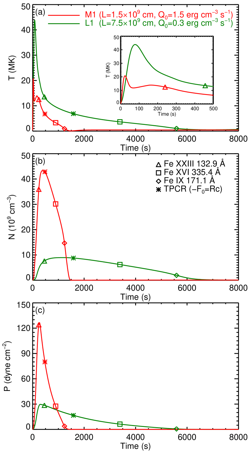
Figure 1: Temporal profiles of the temperature (a), density (b), and pressure (c) in loops M1 (red) and L1 (dark green). The inset in panel (a) gives a zoom-in view of the temperature evolution during the first 500 s. The triangle, square, and diamond mark the properties at the times of line irradiance peaks in Fe XXIII 132.9 Å, Fe XVI 335.4 Å, and Fe IX 171.1 Å, respectively, and the asterisk outlines the transition point from conductive-dominated cooling to radiative-dominated cooling (TPCR) in loop.

Figure 1 shows the temporal evolution of the temperature, density, and pressure in two representative loops (the first loop in experiment 1, typically a main flaring loop, hereafter M1, and the fifth loop in the experiment, typically a late-phase loop, hereafter L1) in response to the corresponding heating pulse. It is clearly seen that the short loop M1 evolves much faster than the long loop L1. This evolution pattern holds when all other loops are included in the experiment. Of the three parameters, the temperature reaches its maximum first, and the density peaks last. Interestingly, the pressure maximum occurs very close to the end time of the heating pulse at $t=300$ s. For the reason mentioned above, longer loops can attain a higher maximum temperature than shorter loops. As to the density and pressure, it is noted that the two peak values are roughly inversely proportional to the loop half-length.

Based on the output temperature and density, we then synthesize the emissions of the loops in several optically thin EUV lines and passbands as they are observed from a near-Earth perspective (e.g., the SDO). The total loop irradiance in a specific line (as that observed in EVE) is given by

$$I_{\mathrm{Line}}=0.83Ab(X)C(T)\langle\mathrm{EM}\rangle\frac{A}{4\pi d^{2}}\ (\mathrm{erg}\ \mathrm{cm}^{-2}\ \mathrm{s}^{-1}),$$ (4)

where the coefficient 0.83 is the commonly assumed ratio of the hydrogen density to electron density in the solar corona, $Ab(X)$ is the abundance of element $X$ relative to hydrogen, $C(T)$ is the contribution function of the emitting ion under consideration, which can be calculated using the CHIANTI atomic database (Del Zanna et al., 2015), $\langle\mathrm{EM}\rangle=2{n}^{2}L$ is the spatially averaged column emission measure (EM) of the loop, $A$ is the loop cross-sectional area, and $d$ is the Sun-Earth distance. Meanwhile, the total intensity of the loop in an AIA passband can be computed as

$$I_{\mathrm{AIA}}=R(T)\langle\mathrm{EM}\rangle A_{\mathrm{pix}}\ (\mathrm{DN}\ \mathrm{s}^{-1}),$$ (5)

where $R(T)$ is the temperature response function of the AIA passband, and $A_{\mathrm{pix}}$ is the normalized loop cross-sectional area in units of AIA pixel. In this work, we consider three iron lines in EUV wavelengths: Fe XXIII 132.9 Å, Fe XVI 335.4 Å, and Fe IX 171.1 Å, whose peak formation temperatures are 14.1 MK, 2.8 MK, and 0.9 MK, reflecting emissions from hot flaring plasmas, warm corona, and cool background corona, respectively. For a comparison with the EUV line irradiance, we choose the AIA passbands of 131 Å, 335 Å, and 171 Å (hereafter AIA 131, 335, and 171), respectively, the dominant ion of which is either the same as or of a similar formation temperature to that of the corresponding EUV line (O’Dwyer et al., 2010).

The commonly used AIA response functions $R(T)$, like those distributed within the AIA package of Solar Software (SSW), are generated using a coronal abundance (e.g., Fludra & Schmelz, 1999) by default. Moreover, the radiative loss function $\Lambda(T)$ used in EBTEL is also formulated based on the coronal abundance. For consistency, when using Equation (4) to calculate irradiance of the three iron lines, we adopt a typical abundance of iron in the solar corona, e.g., $7\times 10^{-5}$. This will enable us to cross-check data from both EVE and AIA when modeling a real solar flare.

Previous observations have revealed that the effective width of a coronal loop is on the order of 1 Mm (e.g., Aschwanden et al., 2008). With the improvement of spatial resolution, it is believed that finer structures within a loop can be resolved with future instruments. In this sense, the specification of a loop cross-sectional area is somewhat arbitrary. For convenience, in experiment 1 the cross-sectional area of all loops is set to one AIA pixel size, i.e., $0\farcs 6\times 0\farcs 6$, which yields a nominal solid angle $A/d^{2}$ of $8.46\times 10^{-12}$ sr in Equation (4) and a unity of $A_{\mathrm{pix}}$ in Equation (5). In practice, this assumption has also been adopted in modeling thousands of flare loops of a solar flare in AIA observations (e.g., Qiu et al., 2012; Zhu et al., 2018), where the chromospheric light curve (e.g., AIA 1600 Å) of each brightening pixel in flare ribbons is used to construct the heating function in the half-loop (of a cross-sectional area of also one AIA pixel) anchored on that pixel. Choosing other values of $A$ ($A_{\mathrm{pix}}$) does not affect our main results, since according to Equations (4) and (5), it just changes the amplitude of the synthetic light curves by the same factor. In passing, we note that under this assumption, the total energy of the impulsive heating injected into each loop in our experiment is $\sim 1.29\times 10^{27}$ erg for $d=1.5\times 10^{13}$ cm.

Figure 2: Synthetic light curves of loops M1 (left) and L1 (right), with the background emission subtracted. The upper and lower panels show the light curves in three EUV lines and three AIA passbands, respectively. The curves are color-coded and scaled according to the legend in each panel.

Figure 2 displays the background-subtracted synthetic light curves of loops M1 and L1 in the three EUV lines and AIA passbands. For the individual loop, as the loop cools down, the loop emission peaks sequentially in lines/passbands of decreasing temperatures. When comparing the different loops, it is found that the increase in loop half-length not only delays the occurrence time of the emission peak, but also reduces the amplitude of the peak. These effects are more prominent for the cool coronal emissions. For example, in loop M1, the largest irradiance peak occurs in the cool coronal Fe IX 171.1 Å line, while in loop L1, the warm coronal Fe XVI 335.4 Å line contributes the most prominent irradiance, and the peak irradiance in Fe IX 171.1 Å even drops to a level lower than that in the hot coronal Fe XXIII 132.9 Å line. In general, the emission evolution in an AIA passband follows a consistent pattern to that in the corresponding EUV line. The peak times in AIA 335 and AIA 171 are nearly simultaneous (within 1 minute) with those in the Fe XVI 335.4 Å and Fe IX 171.1 Å lines. Nevertheless, the peak in AIA 131 shows a systematic delay up to 7 minutes with respect to the Fe XXIII 132.9 Å peak, which we attribute to a slightly lower formation temperature of Fe XXI 128.8 Å ($\sim$11.2 MK), the line of main contribution, compared to Fe XXIII 132.9 Å, the line of much less contribution, in the hot band of AIA 131.

For a quantitative characterization of the emission pattern of the loops, we mainly focus on the line irradiance behavior because it more physically reflects the underlying hydrodynamic evolution in the loops. We infer the peak times of the line irradiance from the two loops displayed in Figure 2. Meanwhile, we define the transition point from conductive-dominated cooling to radiative-dominated cooling (TPCR) for the loops, which can be mathematically expressed as the time when $-F_{0}=\mathcal{R}_{c}$ holds. The corresponding properties at these times are accordingly overplotted on the temporal profiles in Figure 1. In both loops, (1) the initial cooling process is dominated by conductive cooling, which lasts until the loop temperature has considerably dropped but the density has just decreased slightly from its maximum; (2) the irradiance peaks in different lines lie in different cooling regimes: the peak in the hot Fe XXIII line occurs in the conductive cooling phase when the pressure is close to its maximum, while the peaks in the warm Fe XVI and cool Fe IX lines appear in the radiative cooling phase; and (3) the peaks in the Fe XXIII and Fe XVI lines occur when the density is not far from its maximum, whereas the Fe IX line peaks when the material initially evaporated into the loop has been sufficiently drained.

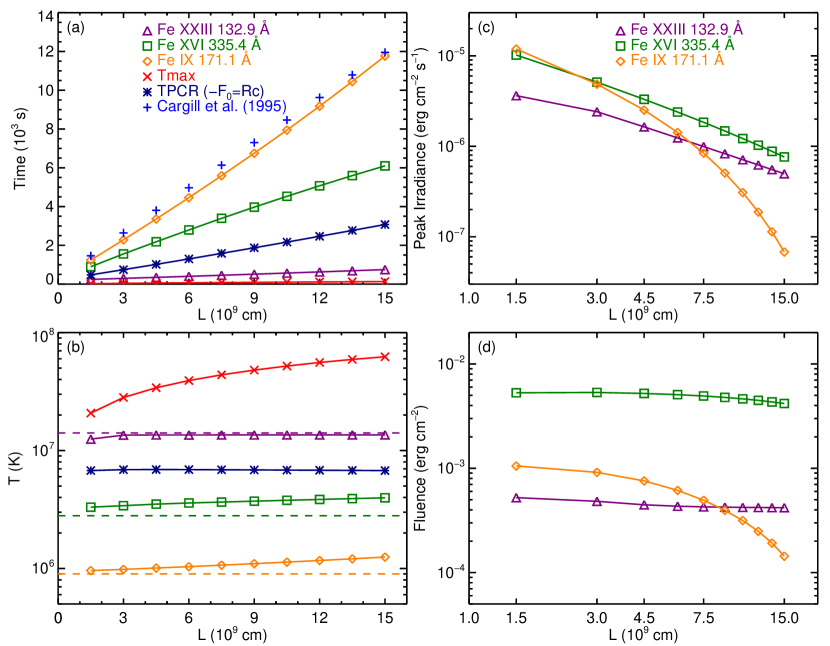
Figure 3: Parameters characterizing the loop emission as functions of the loop half-length for the loops in EBTEL numerical experiment 1. Panel (a) shows the occurrence times of line irradiance peaks, loop maximum temperature, and TPCR, as well as the end time of loop cooling according to Cargill et al. (1995). Panel (b) shows the temperatures at the times of line irradiance peaks and TPCR, as well as the loop maximum temperature itself. The horizontal dashed lines mark the peak formation temperatures of the emitting ions. Panels (c) and (d) depict the background-subtracted peak irradiance and fluence of the three EUV lines, respectively. The meanings of the symbols are explained in the legends.

We further extend our study to all loops in experiment 1 whose emission characteristics as functions of the loop half-length are shown in Figure 3. As expected from the results based on the two-loop sub-sample, for all loops in the experiment, the irradiance peaks in hot and warm/cool lines are divided by the TPCR. The longer the loop, the later occurrence of the peaks, with the peak time nearly linearly proportional to the loop half-length. Furthermore, the cooler the line, the more prominent the delay effect (Figure 3(a)). By assuming a single power-law radiative loss function of $\Lambda(T)\sim T^{-1/2}$ (Rosner et al., 1978) and a temperature$-$density scaling law of $T\sim n^{2}$ during the mass-draining radiative cooling phase (Serio et al., 1991; Jakimiec et al., 1992), Cargill et al. (1995) analytically evaluated the cooling time of a loop (finally cooling down to a temperature $T_{L}$ at which the single power-law of the radiative loss function becomes inaccurate), which is formulated in a ready-to-use form of $\tau_{\mathrm{cool}}=6.06\times 10^{-5}{L^{5/6}}{{p_{0}}^{-1/6}}$ s, where $p_{0}$ is the pressure at the start of the cooling. Here we substitute $p_{0}$ with $p_{\mathrm{max}}$, and rewrite the original formula as

$$\tau_{\mathrm{cool}}=t_{p_{\mathrm{max}}}+6.06\times 10^{-5}\frac{L}{(p_{\mathrm{max}}L)^{1/6}}\ (\mathrm{s}),$$ (6)

where $t_{p_{\mathrm{max}}}$ is the time of maximum pressure, which is very close to $t=300$ s according to the numerical results in experiment 1. The theoretically predicted end times of the cooling in our loop cases derived from Equation (6) are also plotted in Figure 3(a), which show a close proximity to the Fe IX peak times.

The temperatures at the times of line irradiance peaks are in general consistent with the characteristic formation temperatures of the emitting ions (Figure 3(b)). Nonetheless, systematic temperature deviations are also evident to some extent. In the conductive cooling domain, although the loops are all initially heated well above the peak formation temperature of Fe XXIII, the temperature at the time of Fe XXIII irradiance peak is systematically below it. In the radiative cooling regime, the temperatures at the times of Fe XVI and Fe IX irradiance peaks are instead systematically higher than their peak formation temperatures, and furthermore, the deviations are increasingly stronger as the loop half-length increases. It is worth noting that in all loops radiation starts to dominate over the loop cooling at an almost constant temperature of around 6.8 MK.

The background-subtracted peak irradiance for all three EUV lines drops monotonically as the loop half-length increases. (Note that the background levels are orders of magnitude lower than the peak values so that the effect of background-subtraction is actually negligible.) However, the irradiance decreases are quite different in the different lines, as reflected by the different slopes of the curves in Figure 3(c). Except for the first data point in each curve, the peak irradiance in both Fe XXIII and Fe XVI very closely follows a power-law dependence on the loop half-length (straight lines in the $\log-\log$ plotting). The fitted power-law index for Fe XXIII curve is $-0.98$, which means that the Fe XXIII peak irradiance is excellently inversely proportional to the loop half-length. The Fe XVI curve is slightly more sloped, with a fitted index of $-1.18$. The Fe IX peak irradiance, however, deviates from the power-law dependence and decreases much more quickly, changing from the strongest to the weakest irradiance with the increase in loop half-length.

We also compute the line fluence by integrating the background-subtracted line irradiance over the whole loop evolution cycle. It is found that the fluence of Fe XXIII and Fe XVI remains at a relatively flattened level regardless of the loop half-length, while the Fe IX fluence drops by almost an order of magnitude (Figure 3(d)). Since the total amount of energy injected into each loop is constant, this means that the increase in loop half-length greatly reduces the contribution of the cool coronal emissions to the total radiation output from the loop while not obviously affecting those of the hot and warm coronal emissions. In the following, these loop emission characteristics are further investigated in terms of an overall heating-cooling cycle of the loops.

3.2 Experiment 2: Effect of the Heating Rate

It has also been proposed that the EUV late phase is powered by a secondary energy release into the long late-phase loops, which is considerably delayed from the main phase heating and therefore should be much less energetic (Woods et al., 2011; Hock et al., 2012; Dai et al., 2013). In numerical experiment 2, we study the long loops. By adjusting the amplitude of the heating pulse, we probe how the heating rate affects the loop emission properties.

The parameters in experiment 2 are listed in the lower rows of Table 1. The first loop in experiment 2 is exactly the same as loop L1 in experiment 1, which we take as the reference loop. By fixing the loop half-length to be $7.5\times 10^{9}$ cm, we consecutively reduce the peak rate of the impulsive heating by a factor of 3.16 ($10^{1/2}$). Meanwhile, to compensate for the decrease in the total energy deposition rate ($2QL$), we accordingly increase the loop cross-sectional area by the same factor. This factor is equivalent to the number of loops/strands if we assume that the elementary loop has a constant cross-section, as mentioned above. Therefore, the total energy input is unchanged for all the cases in experiment 2, which is also the same as in experiment 1. Note that for the fifth and last loop in the experiment, which we refer to as loop L2, the amplitude of the heating pulse is still 300 times larger than the background heating rate.

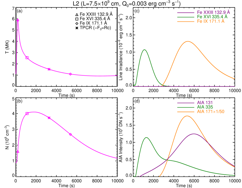
Figure 4: Left: Temporal profiles of the temperature (a) and density (b) in loop L2. Right: Background-subtracted synthetic light curves of loop L2 in the three EUV lines (c) and AIA passbands (d). The left column is organized similarly to Figure 1 and the right column to Figure 2.

Figure 4 shows the temporal evolution of the temperature and density in loop L2, as well as the synthesized background-subtracted light curves in the three EUV lines and AIA passbands. Compared with loop L1 (Figure 1), the heating rate in loop L2 is 100 times lower, and therefore both the temperature and density there evolve relatively more slowly. More importantly, the amplitudes of increase in both quantities are much smaller in loop L2 (Figures 4(a) and (b)) than those in loop L1. The maximum temperature of loop L2 is only 5.9 MK, well below the typical temperatures of hot flaring plasmas ($>10$ MK).

From the synthetic light curves, it is found that the hot Fe XXIII line irradiance from loop L2 is totally “invisible” (although its peak irradiance is orders of magnitude larger than the background level), as expected from the significantly lower loop temperature relative to the peak formation temperature of Fe XXIII. Regarding the emissions of lower temperatures, the peak irradiance of loop L2 in the warm Fe XVI line decreases slightly as compared with the case of loop L1, whereas the peak irradiance in the cool Fe IX line increases slightly. As a result, the relative strengths of the two lines are just reversed for the two loops (Figure 4(c)). Interestingly, it is also found that in loop L2, the peak time of Fe XVI line irradiance moves closer to the time of impulsive heating, 2280 s earlier than that for loop L1, while the occurrence time of Fe IX irradiance peak remains relatively unchanged (within 300 s for the two loops). When we overplot the corresponding properties at the times of line irradiance peaks and TPCR on the temporal profiles in Figures 4(a) and (b), it is clearly seen that in loop L2, the Fe XVI irradiance peak has moved to the conductive cooling regime, near the time of maximum density. Although the Fe IX irradiance peak still remains in the radiative cooling phase, it is shifted somewhat toward the density maximum.

Like that in experiment 1, the light curve in an AIA passband is generally consistent with that in the corresponding EUV line (Figure 4(d)). An exception occurs in AIA 131, in which the intensity peak even lags the AIA 171 peak, reflecting a major contribution from the even cooler lines Fe VIII 130.9/131.2 Å ($\sim 0.6$ MK) rather than Fe XXI 128.8 Å in this passband under the condition of lower loop temperatures. Note that for the convenience of comparison, the light curves of loops L1 (Figures 2(c) and (d)) and L2 (Figures 4(c) and (d)) are plotted within the same ranges.

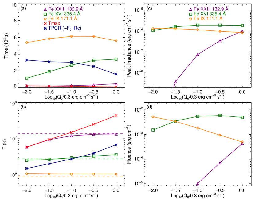
Figure 5: Parameters characterizing the loop emission as functions of the peak heating rate for the loops in EBTEL numerical experiment 2. The panels are organized in the same way as in Figure 3.

The emission characteristics as functions of the peak heating rate for the loops in experiment 2 are displayed in Figure 5. Note that the rightmost data point in each curve refers to the corresponding property in the reference loop L1. As the peak heating rate decreases, the peak time of Fe XVI line irradiance moves monotonically toward the time of heating pulse, while the time of TPCR exhibits an opposite tendency. As a result, the location of the Fe XVI irradiance peak experiences a transition from the radiative cooling domain to the conductive cooling domain (Figure 5(a)). Following this transition, the temperature at the Fe XVI irradiance peak decreases accordingly, changing from slightly above the peak formation temperature of the line to slightly below it (Figure 5(b)). Since the loop maximum temperature drops dramatically with the decrease in heating rate, the occurrence of the Fe XXIII irradiance peak, if it could be observed, finally lies within the time period of the loop maximum temperature. The Fe IX irradiance peak, nevertheless, occurs at a nearly constant temperature of $1.1$ MK, slightly but systematically higher than the peak formation temperature of the line; its occurrence time varies just in a narrow range in the radiative cooling regime.

As to the amplitude of the emissions, the decrease in heating rate only marginally affects the peak irradiance of Fe XVI and Fe IX. The peak irradiance of Fe XVI first is constant and then decreases slightly, while that of Fe IX continues to increase, although the increase extent is very small (Figure 5(c)). When considering the line fluence, this effect becomes obviously exaggerated. As the peak heating rate decreases, the fluence of Fe XVI drops by a factor of 3.3, whereas the Fe IX fluence increases by an order of magnitude (Figure 5(d)). In addition, with the decrease in heating rate, not only the peak irradiance, but also the fluence of Fe XXIII are depressed well below the detectable level.

3.3 Synthesis of an EUV Late-Phase Flare

The actual emission of a solar flare should consist of the contributions from a series of flare loops that have different lengths and/or undergo different energy release processes. Observationally, the length of a flare loop can be measured from spatially revolved imaging observations, and the heating function in that loop can be inferred from the chromospheric light curve at its footpoint, as done in Li et al. (2014b) and Zhu et al. (2018). As a specific type of solar flares, previous case studies have pointed out that the emission of an EUV late-phase flare comes from two sets of flare loops distinct in length (Hock et al., 2012; Dai et al., 2013; Liu et al., 2013a, 2015; Sun et al., 2013; Masson et al., 2017). For simplicity, in this work we just pick up one short main flaring loop and one long late-phase loop from our numerical experiments, and combine their emissions together to synthesize an EUV late-phase flare. Here our main concern is the general shape rather than the absolute amplitude of the flare light curves.

Motivated by the two scenarios in producing the EUV late phase, we consider two cases. In the first case (hereafter Case 1), we directly add the background-subtracted synthetic light curves of loops M1 (Figures 2(a) and (b)) and L1 (Figures 2(c) and (d)) together, assuming that both loops are heated simultaneously and the partition of energy input is 1:1 between the two loops. In the second case (hereafter Case 2), we select loops M1 and L2 (Figures 4(c) and (d)) and assume a time delay in the heating between them. We thus first shift the light curve of loop L2 to a later time by 2000 s. This time delay is based on the time difference of the Fe XVI irradiance peaks (2280 s) between loops L1 and L2 found in numerical experiment 2. In this case, the total amount of energy injected into the late-phase loop L2 is also the same as that into the main flaring loop M1, although the total energy deposition rate in loop L2 is much lower.

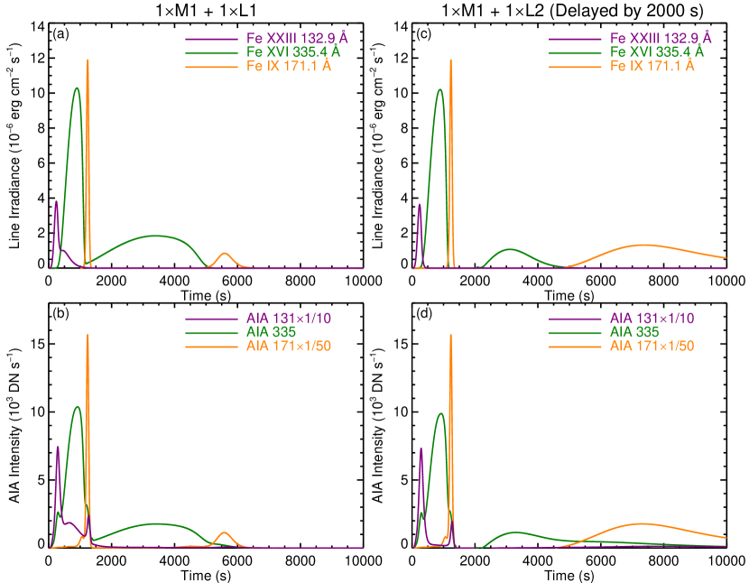
Figure 6: Synthetic light curves of the flare loops mimicking EUV late-phase solar flares produced in two different processes. The light curves are generated by adding the corresponding emission of loop L1 (Case 1, left) or L2 (Case 2, right) to that of loop M1, respectively. In Case 2, the light curve of loop L2 is assumed to be delayed by 2000 s. The upper and lower panels show the light curves in the three EUV lines and AIA passbands, respectively. In all the curves, the background emission has been subtracted.

The synthetic light curves of the two flare cases are shown in Figure 6. For the EUV line irradiance (Figures 6(a) and (c)), both cases exhibit an evident late phase-peak in the warm Fe XVI line, which occurs 42 (37) minutes after the corresponding main flare peak with an irradiance peak ratio of 0.18 (0.10) in Case 1 (2). These properties are in good agreement with those previously found both in statistics (Woods et al., 2011) and case studies (Hock et al., 2012; Dai et al., 2013; Liu et al., 2013a, 2015; Sun et al., 2013). In spite of general similarity, there is also an obvious difference between the Fe XVI late phases in the two cases. In Case 1, the evolution of the late phase in Fe XVI reveals a slow rise and then a fast decay, while the late-phase evolution in Case 2 shows an opposite pattern.

It is also noted that both cases show a secondary late-phase peak in the cool Fe IX line that occurs 37 (71) minutes after the late phase peak of Fe XVI in Case 1 (2). Compared with that in Case 1, the late-phase of Fe IX in Case 2 is more prominent and prolonged. The irradiance in the hot Fe XXIII line, however, exhibits just one main flare peak in both cases. In Case 1, the Fe XXIII peaks in the short loop M1 and long loop L1 occur very close in time, therefore being merged into one main peak followed by a small bump in the composite light curve. In Case 2, the Fe XXIII main peak is purely contributed by loop M1 because at that time the irradiance from loop L2 is still at the background level. The late-phase heating, which goes into loop L2 more than half an hour later, is nevertheless not strong enough to power a detectable enhancement of the Fe XXIII irradiance again.

As to the AIA intensities (Figures 6(b) and (d)), in both cases, the light curves generally resemble those in the corresponding EUV line. The main difference is that there are two peaks in AIA 131 separated by an interval of only 16 minutes (in both cases). At first glance, the second peak in AIA 131 may be regarded as a late-phase peak in the hot coronal emissions by mistake. A further investigation indicates that this peak mainly comes from loop M1 and takes place very shortly after the main flare peak in AIA 171 (also see Figure 2(b)). Therefore, the appearance of the two peaks in AIA 131 in fact reflects a broad coverage of both high and low temperatures in this passband (O’Dwyer et al., 2010), as pointed out above.

4 DISCUSSION

Thanks to the high-quality observations in EUV wavelengths with both full spectral coverage and multiple passband imaging provided by the recently launched SDO mission, the EUV late-phase emission has been discovered, which is seen as a second peak in the warm coronal emissions well after the main flare peak (Woods et al., 2011). These EUV emissions, combined with those formed at higher and lower temperatures, shed light on the hydrodynamic and thermodynamic evolution of the flare loops. The loop properties, such as temperature and density, are actually not uniformly distributed along a flare loop. Nevertheless, since we usually search for an EUV late phase from the loop-integrated light curves of a solar flare, the approach of adopting a 0D model to study the evolution of mean parameters of the flare loop is physically acceptable. There have been a number of 0D hydrodynamic models of coronal loops/strands (Cargill et al., 2012b). In this work, we adopt the EBTEL model (Klimchuk et al., 2008; Cargill et al., 2012a; Barnes et al., 2016) to numerically probe the production of EUV late-phase flares. Through a series of tests of the evolution of loops with different lengths and under different heating processes (Klimchuk et al., 2008; Cargill et al., 2012a), it has been proven that the EBTEL model gives results that agree quite well with those from much more sophisticated 1D simulations such as ARGOS (Antiochos et al., 1999) and HYDRAD (Bradshaw & Mason, 2003; Bradshaw & Klimchuk, 2011), while the computation time is saved by orders of magnitude. In practice, the EBTEL model has also been used both in case studies (Hock et al., 2012; Sun et al., 2013) and parametric surveys (Li et al., 2014a) to reveal the nature of the EUV late phase.

4.1 Emission Characteristics of the Loops

Based on the two explanations of the EUV late phase, i.e., long-lasting cooling and secondary heating, we have carried out two groups of numerical experiments to study the effects of these two processes on the loop emission characteristics. Figure 7(a) displays the temperature$-$density phase plot in an absolute scale for the loops in experiment 1, which depicts an overall heating-cooling cycle of the loops (in the clockwise direction): a fast temperature increase during the impulsive heating, followed by a conductive cooling with plasma evaporation and then a radiative cooling with mass draining, and finally a recovery to the initial equilibrium by the background heating. Although a higher maximum temperature is attained in a longer loop, the greater loop length increases the conductive cooling time $\tau_{c}$, assuming that the pressure is constant during the conductive cooling phase (Antiochos & Sturrock, 1978). During the radiative cooling phase, the lower density in the longer loop also results in a longer radiative cooling time $\tau_{r}$ (Antiochos, 1980). When these two factors are combined, a significant difference in the overall cooling rate is expected between loops with distinct lengths, which naturally explains the delayed occurrence of an EUV late-phase emission.

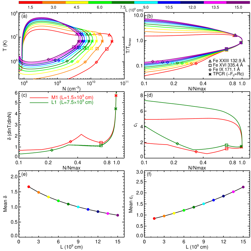
Figure 7: Top: Temperature$-$density phase plot for the loops in EBTEL numerical experiment 1 in absolute scale (a) and normalized scale (b), respectively, where the temperature and density are normalized with respect to the corresponding values at the time of maximum density. Loops with different half-lengths are color-coded with the color bar attached above. The meanings of the symbols are explained in the legend of panel (b). Middle: Evolution of the power index $\delta$ (characterizing the scaling relationship $T\sim n^{\delta}$) during the radiative cooling phase (c) and the parameter $c_{1}$ in the EBTEL model (d) as functions of the normalized density for loops M1 (red) and L1 (dark green), respectively. Bottom: Average values of $\delta$ (e) and $c_{1}$ (f) for all loops over a time interval between the irradiance peaks of Fe XVI (square) and Fe IX (diamond).

According to Equation (4), the variation of line irradiance from a dynamically cooling loop is determined by the evolution of the temperature and density of the loop. In the conductive cooling phase, the density continues to increase when the temperature has passed through the value corresponding to the peak contribution function; thus the line irradiance will continue to increase until the role of the decrease in the contribution function finally overtakes the role of density increase. This causes the irradiance peak to appear at a temperature systematically below the peak formation temperature of the line, while in the radiative cooling phase, as the density continues to decrease, the line irradiance has already reached its peak before the loop cools down to the peak formation temperature of the line. This emission pattern is consistent to what we have found in Figure 3(b).

Strictly speaking, according to Equation (1), the time when the density reaches its maximum should be defined as the time when $-F_{0}=c_{1}\mathcal{R}_{c}$ is satisfied. This time is, indeed, very close to the time of TPCR (as can been seen in Figure 7(a)), since at this time, the parameter $c_{1}$ is close to 1 (as confirmed in Figure 7(d)). Quantitatively, the temperature at the time of maximum density lies in a narrow range around 8 MK for all loops in experiment 1, slightly higher than that (6.8 MK) at the time of TPCR. Therefore, it is reasonable to redraw the temperature$-$density phase plot by normalizing the density and temperature with respect to the corresponding values at the time of maximum density, as shown in Figure 7(b), in which all curves pass through a common point of $(1,1)$.

As seen in the figure, all loops generally exhibit a self-similar evolution in the time period between the irradiance peaks of Fe XXIII and Fe XVI. At the time of Fe XXIII irradiance peak, the column density of internal energy in the loops ($3pL$) is indeed very close to the column density of total heating energy ($Q_{0}L\tau_{H}$), because the radiative loss is almost negligible during that period (except for loop M1, where a considerable amount of energy has been radiated away). Considering that the temperature at the time of Fe XXIII irradiance peak is nearly the same among the loops, we can easily derive a density$-$length relationship of $nL\sim\mathrm{constant}$ and therefore a relationship of $\langle\mathrm{EM}\rangle=2{n}^{2}L\sim L^{-1}$ at this time. According to Equation (4), this results in a perfect inverse relationship between the Fe XXIII peak irradiance and the loop half-length, as shown in Figure 3(c). The density$-$length relationship holds until the time of the Fe XVI irradiance peak, at which the temperature becomes to differ slightly from each other and longer loops tend to have a higher temperature. In this situation, the difference in the contribution function also plays a role, causing the Fe XVI curve in Figure 3(c) to slope slightly more.

After the Fe XVI irradiance peak, the loop evolutions begin to deviate from each other. For the same temperature decrease, the relative density decrease is more significant in longer loops, which can be inferred from the slopes of the curves in Figure 7(b). The density dependence of the curve slope $d\ln T/d\ln n$, which is equal to the power index $\delta$ of the scaling relationship $T\sim n^{\delta}$ during the radiative cooling phase, is shown in Figure 7(c) for loops M1 and L1. The values of $\delta$ for the long loop L1 are systematically lower than those for the short loop M1 during the whole radiative cooling phase. By averaging the values of $\delta$ over an interval between the times of corresponding peaks of Fe XVI and Fe IX, we derive mean $\delta$ values of 1.67 and 1.09 for loops M1 and L1, respectively. Using the full 1D HYDRAD code, Bradshaw & Cargill (2010) numerically studied the mass-draining radiative cooling process of loops with different lengths, revealing a $\delta$ value around 2 for short loops ($2L=2\times 10^{9}$ cm) and a reduced value to about 1 for very long loops (e.g., $2L=2\times 10^{10}$ cm), which are in good agreement with our 0D EBTEL results. In addition, assuming that during the radiative cooling stage the TR radiation is purely maintained by a downward enthalpy flow, Bradshaw & Cargill (2010) also gave an analytical expression of $\delta$, which we rewrite as $\delta=\gamma-1+1/c_{1}$, where $\gamma=5/3$. This formula qualitatively implies a larger $\delta$ caused by a smaller $c_{1}$, and vice versa. In Figure 7(d), we compare the evolution of the EBTEL parameter $c_{1}$ for loops M1 and L1, and find that this is indeed the case. During the whole loop evolution, the $c_{1}$ values for loop L1 are always higher than those for loop M1. The reason just lies in the new physics included in the improved EBTEL model. With a higher ratio of the loop length to the gravitational scale height, the radiative loss of loop L1 from the corona is more significantly depressed by the gravitational stratification, leading to higher values of $c_{1}$ in loop L1 than those in loop M1.

In Figures 7(e) and (f), we plot the mean values of $\delta$ and $c_{1}$ for all loops in experiment 1, respectively. As expected, as the loop length increases, the mean $\delta$ value ($\bar{\delta}$) decreases monotonically from 1.67 to 0.73, while the mean $c_{1}$ value ($\bar{c}_{1}$) increases monotonically from 0.84 to 2.26. We do not seek to build a quantitative relationship between $\bar{\delta}$ and $\bar{c}_{1}$, because the contribution of the heat flux has not been evaluated, although the role of thermal conduction in this stage should be marginal.

Since the loop evolution diverges after the Fe XVI irradiance peak, the peak irradiance of Fe IX no longer follows a power-law dependence, but drops much more quickly with the increase in loop half-length (see Figure 3(c)), and the fluence of Fe IX is also greatly depressed, as opposed that of to the Fe XXIII and Fe XVI lines (see Figure 3(d)). For the same reason, the line irradiance in long loop peaks in the radiative cooling domain at a higher temperature than that in a short loop, as also shown in Figure 3(b).

In a case study of two EUV late-phase flares, Liu et al. (2013a) used the Cargill et al. (1995) formula to estimate the cooling times of the late-phase loops, which are qualitatively consistent with the observed time delays in Fe IX irradiance peak. In this work, we rewrite the original Cargill et al. (1995) formula as Equation (6). According to the parameters in experiment 1, at the start of the cooling (the time of maximum pressure), the quantity $p_{\mathrm{max}}L$ is approximately constant among all the loops, except for loop M1 where $p_{\mathrm{max}}L$ is 15% lower. This fluctuation of $p_{\mathrm{max}}L$ has only little influence on the cooling time. Therefore, a linear relationship between the cooling time and the loop half-length is expected, just as shown in Figure 3(a). Interestingly, the theoretically predicted end time of the loop cooling shows a close proximity to the time of Fe IX irradiance peak for the corresponding experiment loop. In the EBTEL model, the radiative loss function is given in a piecewise continuous form (Klimchuk et al., 2008), and the temperature$-$density scaling relationship changes from $T\sim n^{2}$ for short loops to $T\sim n$ for long loops according to our experiment. Both values are different from the assumptions adopted in Cargill et al. (1995). The surprisingly excellent consistency between the results of the two approaches implies that the shape of radiative loss function and gravity may have a significant effect on the amplitude of the loop parameters, but they do not considerably affect the timing of the loop evolution. Although EBTEL is just a simplified 0D model, it can still help us capture some essential characteristics of the flare evolution in case studies.

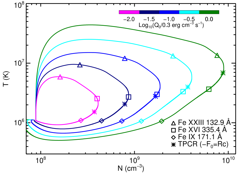
Figure 8: Temperature$-$density phase plot for the loops in EBTEL numerical experiment 2 in absolute scale. Loops heated with different amplitudes are color-coded. The meanings of the symbols are the same as in Figure 7.

Figure 8 displays the temperature$-$density phase plot in an absolute scale for the loops in experiment 2. The maximum temperature itself and the temperatures at the times of maximum density and TPCR both drop considerably as the heating rate decreases, as also shown in Figure 5(b). Therefore, normalization of the temperature$-$density phase plot, as done for the loops in experiment 1, is physically not applicable in this experiment. To be precise, quantitatively probing the emission characteristics of loops in experiment 2 is not as straightforward as what we have done for the loops in experiment 1. Qualitatively, we propose that temperature is a decisive factor in this experiment.

As the loop maximum temperature decreases to well below those of hot flaring plasmas, i.e., $\sim 10$ MK, the irradiance of hot coronal lines, e.g., Fe XXIII, is totally depressed to an undetectable level. Nevertheless, even with the least energetic heating, the loop can still attain a sufficiently high maximum temperature of about $6$ MK, which guarantees the appearance of a sufficiently prominent irradiance peak in the warm Fe XVI line. Different from that in experiment 1, the Fe XVI irradiance peak has gradually moved to the conductive cooling domain in experiment 2. Since in the conductive cooling phase the cooling rate is relatively faster, the peak time of Fe XVI irradiance closer approaches the time of heating pulse, indicating a prompt response of the warm coronal emissions to the late-phase heating. Meanwhile, the temperature at the time of Fe XVI irradiance peak drops below the peak formation temperature of the line. Considering that the radiation output from the loop has now moved to lower temperatures, the irradiance of the cool Fe IX line is certainly enhanced. All these emission characteristics are shown in Figure 5.

Finally, according to Equation (6), the Fe IX peak time should be postponed as the heating rate decreases, since the quantity $p_{\mathrm{max}}L$ decreases accordingly. However, this is not the case in experiment 2, as seen in Figure 5(a). The reason is that the condition for the Cargill et al. (1995) formula to hold, $T_{H}\gg T_{L}$, (where $T_{H}$ and $T_{L}$ are the temperatures at the start and end of the cooling, respectively,) is no longer satisfied.

4.2 Production of the EUV Late Phase

By combining the emissions from a short main flaring loop and a long late-phase loop in our numerical experiments, we have synthesized the light curves of two cases mimicking the EUV late phase flares produced in two different processes. As seen in Figure 6, both cases exhibit an EUV late-phase in the warm Fe XVI line. Case 1 is based on the long-lasting cooling scenario. The difference in cooling time for Fe XVI between the two loops of distinct lengths is indeed large enough to separate the late-phase peak from the main flare peak, while for the hot Fe XXIII line, the peaks in two loops are merged into one because the cooling rate is still very fast in the long loop during the conductive cooling phase. However, a small bump is produced following the main flare peak in the composite Fe XXIII light curve. Since the SXR emissions are formed at a similar temperature to that of Fe XXIII, we would see a similar dual-decay behavior in the corresponding GOES SXR light curve. We note that this dual-decay behavior in GOES SXRs has been used as a proxy for EUV late-phase flares prior to theSDO era (Woods, 2014). Case 2 is in accordance with the secondary heating scenario. The late-phase heating produces a rather prompt enhancement of the Fe XVI emission in the long late-phase loop. However, the amplitude of the heating is too small to raise the temperature to that required for the formation of detectable Fe XXIII emission.

As seen from the temperature$-$density phase plot in Figures 7 and 8, the density at the Fe XVI irradiance peak in the late-phase loop is not far from its maximum value in both cases. The large enough density guarantees a sufficiently strong Fe XVI late-phase peak, which can be readily observed. In addition, we also note that the late-phase peaks in the two cases occur in different cooling domains. In Case 1, the late-phase peak occurs during the radiative cooling phase. After this, the irradiance is notably affected by the fast mass draining, therefore showing a fast decay. In Case 2, however, the late phase-peak takes place during the conductive cooling phase when the density is still increasing. The decay phase in Case 2 is thus more gradual than the rise phase. Li et al. (2014a) have proposed two preliminary methods to determine whether or not a secondary heating plays a role in the late-phase emission. Here, we propose a new method to diagnose the processes behind an EUV late phase, which is based on the shape of light curves of warm coronal emissions. Light curves with a slow rise followed by a fast decay favor the long-lasting cooling scenario, whereas those showing an opposite pattern are more likely due to the secondary heating process.

We have applied this method to diagnosing a series of EUV late-phase flares occurring in 2011 September from NOAA AR 11283. The production of EUV late phase in the X2.1 class eruptive flare on September 6 has been investigated by Dai et al. (2013), who found convincing evidence for a late energy injection into the the late-phase loops. The late-phase light curves in both EVE 335 Å and AIA 335 Å (Figures 1 and 4 in their paper) reveal a more gradual decay than the rise. In another M1.2 class non-eruptive flare on 2011 September 9 (Y.Dai et al. 2018, in preparation), it is found the the late-phase loops undergo an intense heating even 5 minutes earlier than the main flare heating. Both the overall late-phase light curve and the light curve extracted from a single late phase loop in Fe XVI show a relatively faster decay than the rise. These evolution patterns are in quality consistent with our expectation, and the detailed results will be presented in a separate paper.

Even with an equal energy partition between the main flaring loop and late-phase loop, the irradiance ratios of the late-phase peak to main flare peak are still only 0.18 and 0.1 for the two cases in our experiments, because the long length of the late-phase loop significantly reduces the line peak irradiance from the loop. In diagnosing the flares from AR 11283, we also note that not all flares from this AR exhibit an evident EUV late phase, even though the flare class is sufficiently high. In a real solar flare, it is very rare that the late-phase loops, if they do exist, receive a total energy input comparable to or greater than that the input into the main flaring loops. Even if an EUV late phase is produced in the late-phase loops, the late-phase emission may be too weak to be observed. In addition to the reason pinpointed in Li et al. (2014a), this may be another reason why EUV late-phase flares only occupy a small fraction in all solar flares. In passing, we note that Liu et al. (2015) have recently reported an extremely large EUV late phase (an even greater late-phase peak than the main flare peak) in a confined solar flare, attributing the production of this extremely large late phase to the persistent heating powered by a trapped hot structure (most presumably a flux rope).

There are still some other factors that we did not includ in our numerical modeling, which may potentially affect the loop emissions. The first one is nonthermal electron beam heating, whose effect has been addressed in Liu et al. (2013b) by using the EBTEL model. Nevertheless, many observations with RHESSI (Lin et al., 2002) have shown that HXR emissions, which are believed to be produced by the bremsstrahlung of nonthermal electrons in the solar lower atmosphere (e.g., Hao et al., 2017), mainly come from the footpoints of short main flaring loops rather than long late-phase loops (e.g., Feng et al., 2013; Sun et al., 2013). The second factor is deviations from ionization equilibrium (Reale & Orlando, 2008; Bradshaw & Klimchuk, 2011). During the impulsive heating and conductive cooling stage, the temperature evolves so fast that the ionization process cannot catch up with the temperature variation, resulting in a non-equilibrium ionization. Obviously, this effect is the most prominent for hot coronal lines in long tenuous loops. As Bradshaw & Klimchuk (2011) have pointed out, as the cooling rate slows down and the density increases, the ions can have enough time to reach an ionization equilibrium at a medium temperature like 6 MK. Therefore the emissions formed below this temperature are unlikely to be notably affected by this effect. The last factor is CME-associated coronal dimming (Aschwanden et al., 2009; Cheng & Qiu, 2016). Of the two synthetic EUV late-phase flares, the late phase of the cool Fe IX line in Case 1 is quite weak because of the fast mass draining in this stage, while the late phase in Case 2 is rather prominent. According to previous case studies (Hock et al., 2012; Dai et al., 2013), Case 2 is more likely to correspond to an eruptive flare, in which the late-phase heating is caused by magnetic reconnection between the magnetic field lines stretched out by the eruption of a flux rope near the time of main flare peak (Cheng et al., 2017). Mass depletion accompanying the CME lift-off will cause a prolonged coronal dimming in the bulk coronal emission, which easily submerges the cool coronal late phase. Emissions of higher temperatures, however, are little affected by this dimming, because they contribute only very little to the bulk coronal emission. To summarize, none of these factors may impose a notable effect on the EUV late-phase emission, as it comes from loops of great lengths and medium temperatures. This may answer the question why the EUV late phase is mainly observed in warm coronal emissions.

5 SUMMARY

Using the EBTEL model, we have numerically synthesized two flare cases that mimic EUV late-phase solar flares produced via two main mechanisms, i.e., long-lasting cooling and secondary heating mechanisms. We probed in detail the physical link between the emission characteristics and the underlying hydrodynamics and thermodynamics in the flare loops. Our main conclusion is that the underlying hydrodynamic and thermodynamic evolutions in late-phase loops are different if they are generated by the two different mechanisms. The late-phase peak due to a long-lasting cooling process always occurs during the radiative cooling phase, while that powered by a secondary heating is more likely to take place in the conductive cooling phase. We then proposed a new method for diagnosing the two mechanisms based on the shape of late-phase light curves. The preliminary application of the method to real solar observations is encouraging. Moreover, we discussed the energy partition between the different loops in a solar flare, and pointed out that it is not easy for the flare to exhibit an evident EUV late phase. Finally, we also addressed some other factors that may potentially affect the loop emissions. We proposed that none of them may impose a notable effect on the warm coronal late-phase emission.

To better understand the nature of the EUV late phase of solar flares, we need more observations. The MEGS-A component of EVE, whose spectral window covers the EUV lines used in this study, has been lost since 2014 May 26. Fortunately, we still have AIA in good working order. Because of the close similarity between the EUV emissions from the two instruments, as shown in this work, we can reliably extract the late-phase information from a solar flare.

References

- Antiochos (1980) Antiochos, S. K. 1980, ApJ, 241, 385
- Antiochos et al. (1999) Antiochos, S. K., MacNeice, P. J., Spicer, D. S., & Klimchuk, J. A. 1999, ApJ, 512, 985
- Antiochos & Sturrock (1976) Antiochos, S. K., & Sturrock, P. A. 1976, Sol. Phys., 49, 359
- Antiochos & Sturrock (1978) —. 1978, ApJ, 220, 1137
- Aschwanden et al. (2008) Aschwanden, M. J., Nitta, N. V., Wuelser, J.-P., & Lemen, J. R. 2008, ApJ, 680, 1477
- Aschwanden et al. (2009) Aschwanden, M. J., Nitta, N. V., Wuelser, J.-P., et al. 2009, ApJ, 706, 376
- Barnes et al. (2016) Barnes, W. T., Cargill, P. J., & Bradshaw, S. J. 2016, ApJ, 829, 31
- Bradshaw & Cargill (2005) Bradshaw, S. J., & Cargill, P. J. 2005, A&A, 437, 311
- Bradshaw & Cargill (2010) —. 2010, ApJ, 717, 163
- Bradshaw & Klimchuk (2011) Bradshaw, S. J., & Klimchuk, J. A. 2011, ApJS, 194, 26
- Bradshaw & Mason (2003) Bradshaw, S. J., & Mason, H. E. 2003, A&A, 401, 699
- Cargill & Bradshaw (2013) Cargill, P. J., & Bradshaw, S. J. 2013, ApJ, 772, 40
- Cargill et al. (2012a) Cargill, P. J., Bradshaw, S. J., & Klimchuk, J. A. 2012a, ApJ, 752, 161
- Cargill et al. (2012b) —. 2012b, ApJ, 758, 5
- Cargill et al. (1995) Cargill, P. J., Mariska, J. T., & Antiochos, S. K. 1995, ApJ, 439, 1034
- Carmichael (1964) Carmichael, H. 1964, NASA Special Publication, 50, 451
- Chamberlin et al. (2012) Chamberlin, P. C., Milligan, R. O., & Woods, T. N. 2012, Sol. Phys., 279, 23
- Chamberlin et al. (2008) Chamberlin, P. C., Woods, T. N., & Eparvier, F. G. 2008, Space Weather, 6, S05001
- Cheng & Qiu (2016) Cheng, J. X., & Qiu, J. 2016, ApJ, 825, 37
- Cheng et al. (2017) Cheng, X., Guo, Y., & Ding, M. 2017, Science in China Earth Sciences, 60, 1383
- Dai et al. (2013) Dai, Y., Ding, M. D., & Guo, Y. 2013, ApJ, 773, L21
- Del Zanna et al. (2015) Del Zanna, G., Dere, K. P., Young, P. R., Landi, E., & Mason, H. E. 2015, A&A, 582, A56
- Feng et al. (2013) Feng, L., Wiegelmann, T., Su, Y., et al. 2013, ApJ, 765, 37
- Fludra & Schmelz (1999) Fludra, A., & Schmelz, J. T. 1999, A&A, 348, 286
- Guo et al. (2017) Guo, Y., Cheng, X., & Ding, M. 2017, Science in China Earth Sciences, 60, 1408
- Hao et al. (2017) Hao, Q., Yang, K., Cheng, X., et al. 2017, Nature Communications, 8, 2202
- Hirayama (1974) Hirayama, T. 1974, Sol. Phys., 34, 323
- Hock et al. (2012) Hock, R. A., Woods, T. N., Klimchuk, J. A., Eparvier, F. G., & Jones, A. R. 2012, ArXiv e-prints, arXiv:1202.4819
- Jakimiec et al. (1992) Jakimiec, J., Sylwester, B., Sylwester, J., et al. 1992, A&A, 253, 269
- Jiang et al. (2013) Jiang, C., Feng, X., Wu, S. T., & Hu, Q. 2013, ApJ, 771, L30
- Johnston et al. (2017) Johnston, C. D., Hood, A. W., Cargill, P. J., & De Moortel, I. 2017, A&A, 597, A81
- Klimchuk et al. (2008) Klimchuk, J. A., Patsourakos, S., & Cargill, P. J. 2008, ApJ, 682, 1351
- Kopp & Pneuman (1976) Kopp, R. A., & Pneuman, G. W. 1976, Sol. Phys., 50, 85
- Lemen et al. (2012) Lemen, J. R., Title, A. M., Akin, D. J., et al. 2012, Sol. Phys., 275, 17
- Li et al. (2014a) Li, Y., Ding, M. D., Guo, Y., & Dai, Y. 2014a, ApJ, 793, 85
- Li et al. (2012) Li, Y., Qiu, J., & Ding, M. D. 2012, ApJ, 758, 52
- Li et al. (2014b) —. 2014b, ApJ, 781, 120
- Lin et al. (2002) Lin, R. P., Dennis, B. R., Hurford, G. J., et al. 2002, Sol. Phys., 210, 3
- Liu et al. (2015) Liu, K., Wang, Y., Zhang, J., et al. 2015, ApJ, 802, 35
- Liu et al. (2013a) Liu, K., Zhang, J., Wang, Y., & Cheng, X. 2013a, ApJ, 768, 150
- Liu et al. (2013b) Liu, W.-J., Qiu, J., Longcope, D. W., & Caspi, A. 2013b, ApJ, 770, 111
- Martens (2010) Martens, P. C. H. 2010, ApJ, 714, 1290
- Masson et al. (2017) Masson, S., Pariat, É., Valori, G., et al. 2017, A&A, 604, A76
- Neupert (1968) Neupert, W. M. 1968, ApJ, 153, L59
- O’Dwyer et al. (2010) O’Dwyer, B., Del Zanna, G., Mason, H. E., Weber, M. A., & Tripathi, D. 2010, A&A, 521, A21
- Parker (1963) Parker, E. N. 1963, ApJS, 8, 177
- Pesnell et al. (2012) Pesnell, W. D., Thompson, B. J., & Chamberlin, P. C. 2012, Sol. Phys., 275, 3
- Qiu et al. (2012) Qiu, J., Liu, W.-J., & Longcope, D. W. 2012, ApJ, 752, 124
- Reale & Orlando (2008) Reale, F., & Orlando, S. 2008, ApJ, 684, 715
- Rosner et al. (1978) Rosner, R., Tucker, W. H., & Vaiana, G. S. 1978, ApJ, 220, 643
- Serio et al. (1991) Serio, S., Reale, F., Jakimiec, J., Sylwester, B., & Sylwester, J. 1991, A&A, 241, 197
- Sturrock (1966) Sturrock, P. A. 1966, Nature, 211, 695
- Sun et al. (2013) Sun, X., Hoeksema, J. T., Liu, Y., et al. 2013, ApJ, 778, 139
- Tobiska et al. (2000) Tobiska, W. K., Woods, T., Eparvier, F., et al. 2000, Journal of Atmospheric and Solar-Terrestrial Physics, 62, 1233
- Woods (2014) Woods, T. N. 2014, Sol. Phys., 289, 3391
- Woods et al. (2011) Woods, T. N., Hock, R., Eparvier, F., et al. 2011, ApJ, 739, 59
- Woods et al. (2012) Woods, T. N., Eparvier, F. G., Hock, R., et al. 2012, Sol. Phys., 275, 115
- Zhu et al. (2018) Zhu, C., Qiu, J., & Longcope, D. W. 2018, ApJ, 856, 27