Twelve Simple Algorithms to Compute Fibonacci Numbers

Abstract

The Fibonacci numbers are a sequence of integers in which every number after the first two, 0 and 1, is the sum of the two preceding numbers. These numbers are well known and algorithms to compute them are so easy that they are often used in introductory algorithms courses. In this paper, we present twelve of these well-known algorithms and some of their properties. These algorithms, though very simple, illustrate multiple concepts from the algorithms field, so we highlight them. We also present the results of a small-scale experimental comparison of their runtimes on a personal laptop. Finally, we provide a list of homework questions for the students. We hope that this paper can serve as a useful resource for the students learning the basics of algorithms.

1 Introduction

The Fibonacci numbers are a sequence $F_{n}$ of integers in which every number after the first two, 0 and 1, is the sum of the two preceding numbers: $0,1,1,2,3,5,8,13,21,..$. More formally, they are defined by the recurrence relation $F_{n}=F_{n-1}+F_{n-2}$, $n\geq 2$ with the base values $F_{0}=0$ and $F_{1}=1$ [1, 5, 7, 8].

The formal definition of this sequence directly maps to an algorithm to compute the $n$th Fibonacci number $F_{n}$. However, there are many other ways of computing the $n$th Fibonacci number. This paper presents twelve algorithms in total. Each algorithm takes in $n$ and returns $F_{n}$.

Probably due to the simplicity of this sequence, each of the twelve algorithms is also fairly simple. This allows the use of these algorithms for teaching some key concepts from the algorithms field, e.g., see [3] on the use of such algorithms for teaching dynamic programming. This paper is an attempt in this direction. Among other things, the algorithmic concepts illustrated by these algorithms include

• top-down vs. bottom-up dynamic programming [1, 3],

• dynamic programming with vs. without memoization [1, 3],

• recursion vs. iteration [11, 13, 14],

• integer vs. floating-point arithmetic [4, 15],

• exact vs. approximate results [4, 15],

• exponential-time vs. polynomial-time [12],

• constant-time vs. non-constant-time arithmetic [9],

• progression from constant to polynomial to exponential time and space complexity [1, 12],

• closed-form vs. recursive formulas [16],

• repeated squaring vs. linear iteration for exponentiation [1], and

• recursion depth [11, 13, 14].

Given the richness of the field of the Fibonacci numbers, it seems that more algorithmic concepts will be found for illustration in the future using the computation of the Fibonacci numbers.

We present each algorithm as implemented in the Python programming language (so that they are ready-to-run on a computer) together with their time and space complexity analyses. We also present a small-scale experimental comparison of these algorithms. We hope students with an interest in learning algorithms may find this paper useful for these reasons. The simplicity of the algorithms should also help these students to focus on learning the algorithmic concepts illustrated rather than struggling with understanding the details of the algorithms themselves.

Since the Fibonacci sequence has been well studied in math, there are many known relations [8], including the basic recurrence relation introduced above. Some of the algorithms in this study directly implement a known recurrence relation on this sequence. Some others are derived by converting recursion to iteration. In [6], even more algorithms together with their detailed complexity analyses are presented.

Interestingly, there are also closed-form formulas on the Fibonacci numbers. The algorithms derived from these formulas are also part of this study. However, these algorithms produce approximate results beyond a certain $n$ due to their reliance on the floating-point arithmetic.

For convenience, we will refer to the algorithms based on whether or not their results are exact or approximate Fibonacci numbers: Exact algorithms or approximate algorithms.

2 Preliminaries

These are the helper algorithms or functions used by some of the twelve algorithms. Each of these algorithms are already well known in the technical literature [1]. They are also simple to derive.

Note that $m=[[a,b],[c,d]]$ in the Python notation means a 2x2 matrix

$$m=\left(\begin{array}[]{cc}a&b\\ c&d\end{array}\right)$$ (1)

in math notation. Also, each element is marked with its row and column id as in, e.g., $m[0][1]$ in Python notation means $m_{01}=b$ in math notation.

Since we will compute $F_{n}$ for large $n$, the number of bits in $F_{n}$ will be needed. As we will later see,

$$F_{n}=\left[{\frac{\varphi^{n}}{\sqrt{5}}}\right]\text{and }\varphi=\frac{1+\sqrt{5}}{2}\approx 1.618033$$ (2)

where $\varphi$ is called the golden ratio and $[\cdot]$ rounds its argument. Hence, the number of bits in $F_{n}$ is equal to $\lg F_{n}\approx n\lg\varphi\approx 0.7n=\Theta(n)$.

In the sequel, we will use $A(b)$ and $M(b)$ to represent the time complexity of adding (or subtracting) and multiplying (or dividing) two $b$-bit numbers, respectively. For fixed precision arguments with constant width, we will assume that these operations take constant time, i.e., $A(b)=M(b)=O(1)$; we will refer to this case as constant-time arithmetic. For arbitrary precision arguments, $A(b)=O(b)$ and $M(b)=O(b^{2})$, although improved bounds for each exist [9]; we will refer to this case as non-constant-time arithmetic. The non-constant case also applies when we want to express the time complexity in terms of bit operations, even with fixed point arguments. In this paper, we will vary $b$ from 32 to $F_{10,000}$, which is around 7,000 bits per Eq. 2.

What follows next are these helper algorithms, together with their description, and their time complexity analyses in bit operations.

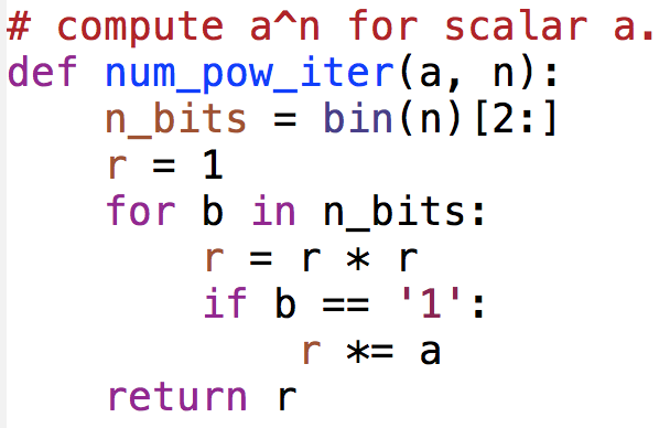
• num_pow_iter(a,n) in Fig. 1: An algorithm to compute $a^{n}$ for floating-point $a$ and non-negative integer $n$ iteratively using repeated squaring, which uses the fact that $a^{n}=(a^{(\frac{n}{2})})^{2}$. This algorithm iterates over the bits of $n$, so it iterates $\lg n$ times. In each iteration, it can multiply two $b$-bit numbers at most twice, where $b$ ranges from $\lg a$ to $\lg a^{n-1}$ in the worst case, or where each iteration takes time from $M(\lg a)$ and $M(\lg a^{n})$. The worst case happens when the bit string of $n$ is all 1s, i.e., when $n$ is one less than a power of 2. As such, a trivial worst-case time complexity is $O(M(\lg a^{n})\lg n)$. However, a more careful analysis shaves off the $\lg n$ factor to lead to $O(M(\lg a^{n}))=O(M(n\lg a))$. With constant-time arithmetic, the time complexity is $O(\lg n)$.

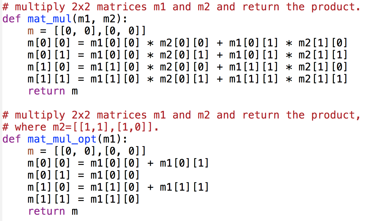
• mat_mul(m1,m2) in Fig. 2: An algorithm to compute the product $m1*m2$ of two 2x2 matrices $m1$ and $m2$. This algorithm has eight multiplications, so the total time complexity is $O(M(max(\lg max(m1),\lg max(m2))))$, where $max(m)$ returns the largest element of the matrix $m$.

• mat_mul_opt(m1) in Fig. 2: An algorithm to compute the product $m1*m2$ of two 2x2 matrices $m1$ and $m2$ when $m2=[[1,1],[1,0]]$, in the Python list notation. This algorithm is an optimized version of mat_mul(m1,m2) in Fig. 2. The total time complexity is then $O(M(\lg max(m1)))$.

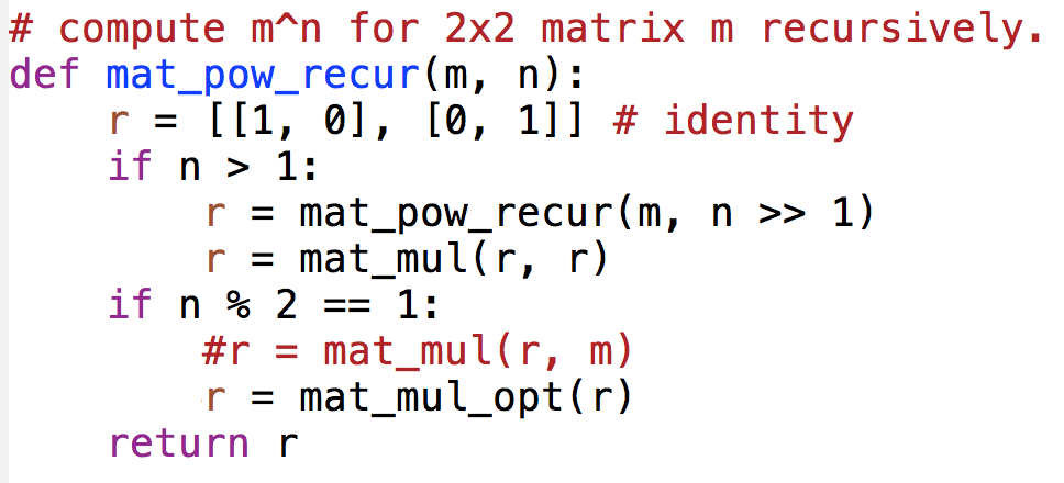
• mat_pow_recur(m,n) in Fig. 3: An algorithm to compute $m^{n}$ of a 2x2 matrix $m$ recursively using repeated squaring. Its time complexity analysis is similar to that of num_pow_iter. As such, the time complexity is $O(M(\lg a))$ where $a=max(r)$. With constant-time arithmetic, the time complexity is $O(\lg n)$.

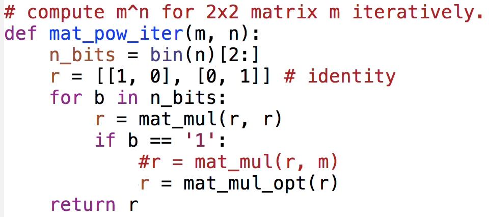
• mat_pow_iter(m,n) in Fig. 4: An algorithm to compute $m^{n}$ of a 2x2 matrix $m$ iteratively using repeated squaring. Its time complexity is equal to that of its recursive version, i.e., $O(M(\lg a))$ where $a=max(r)$. With constant-time arithmetic, the time complexity is $O(\lg n)$.

• negafib(m,Fn) in Fig. 5: An algorithm to return the “negafibonacci” number corresponding to the $n$th Fibonacci number $F_{n}$. A negafibonacci number is a Fibonacci number with a negative index; such numbers are defined as $F_{-n}=(-1)^{n+1}F_{n}$ [8].

• The function round(x) or [x] rounds its floating-point argument to the closest integer. It maps to the math.round(x) function from the standard math library of Python.

Figure 1: num_pow_iter(a,n): An algorithm to compute $a^{n}$ for floating-point $a$ and non-negative integer $n$ iteratively using repeated squaring.

Figure 2: mat_mul(m1,m2): An algorithm to compute the product $m1*m2$ of two 2x2 matrices $m1$ and $m2$. mat_mul_opt(m1) is the optimized version when $m2=[[1,1],[1,0]]$ in the Python list notation.

Figure 3: mat_pow_recur(m,n): An algorithm to compute $m^{n}$ of a 2x2 matrix $m$ for non-negative integer $n$ recursively using repeated squaring.

Figure 4: mat_pow_iter(m,n): An algorithm to compute $m^{n}$ of a 2x2 matrix $m$ for non-negative integer $n$ iteratively using repeated squaring.

Figure 5: negafib(n,Fn): An algorithm to compute the negafibonacci corresponding to $n$th Fibonacci number $F_{n}$.

3 The Twelve Algorithms

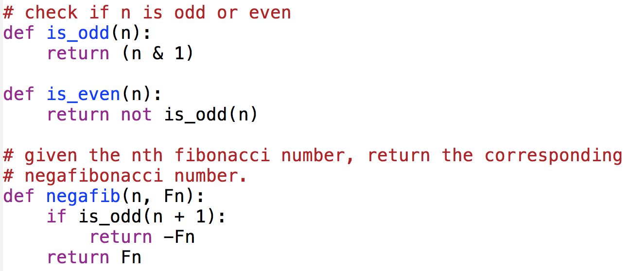
We now present each algorithm, together with a short explanation on how it works, its time and space complexity analyses, and some of the concepts from the algorithms field it illustrates. Each algorithm takes $n$ as the input and returns the $n$th Fibonacci number $F_{n}$. Note that $n$ can also be negative, in which case the returned numbers are called “negafibonacci” numbers, defined as $F_{-n}=(-1)^{n+1}F_{n}$ [9].

Some of the algorithms use a data structure $F$ to cache pre-computed numbers such that $F[n]=F_{n}$. For some algorithms $F$ is an array (a mutable list in Python) whereas for some others it is a hash table (or dictionary in Python). In Python, lists and dictionaries are accessed the same way, so the type of the data structure can be found out by noting whether or not the indices accessed are consecutive or not.

Each algorithm is also structured such that the base cases for $n=0$ to $n=1$ (or $n=2$ in some cases) are taken care of before the main part is run. Also note that some of the algorithms in this section rely on one or more algorithms from the preliminaries section.

Figure 6: fib1(n): An algorithm to compute the $n$th Fibonacci number $F_{n}$ recursively using dynamic programming. This algorithm uses probably the most well-known recurrence relation defining Fibonacci numbers.

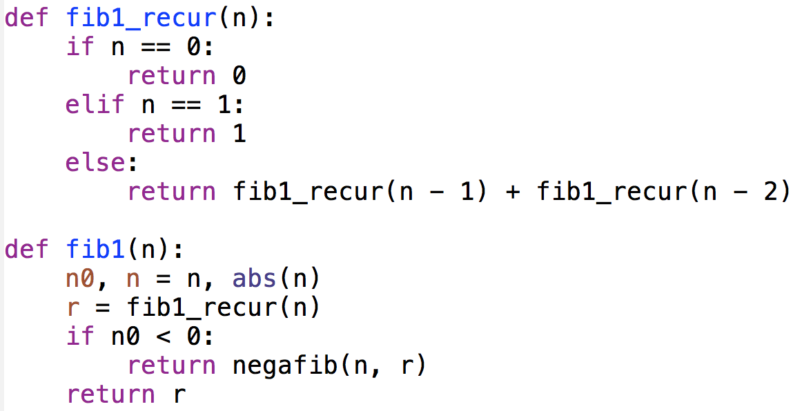
3.1 Algorithm fib1: Top-down Dynamic Programming

fib1 is derived directly from the recursive definition of the Fibonacci sequence: $F_{n}=F_{n-1}+F_{n-2}$, $n\geq 2$, with the base values $F_{0}=0$ and $F_{1}=1$.

Its time complexity $T(n)$ with constant-time arithmetic can be expressed as $T(n)=T_{n-1}+T_{n-2}+1$, $n\geq 2$, with the base values $T(0)=1$ and $T(1)=2$. The solution of this linear non-homogeneous recurrence relation implies that the time complexity is equal to $T(n)=O(F_{n})=O(\varphi^{n})$, which is exponential in $n$.

Its time complexity with non-constant-time arithmetic leads to $T(n)=T_{n-1}+T_{n-2}+A(\lg F_{n-1})$, where the last term signifying the cost of the addition run in $O(n)$ time. The solution of this linear non-homogeneous recurrence relation implies that the time complexity is also equal to $T(n)=O(F_{n})=O(\varphi^{n})$, which is also exponential in $n$.

The space complexity for each case above has the same exponential dependence on $n$.

Regarding algorithmic concepts, fib1 illustrates recursion, top-down dynamic programming, and exponential complexity.

Figure 7: fib2(n): An algorithm to compute the $n$th Fibonacci number $F_{n}$ recursively using dynamic programming with memoization (i.e., caching of pre-computed results).

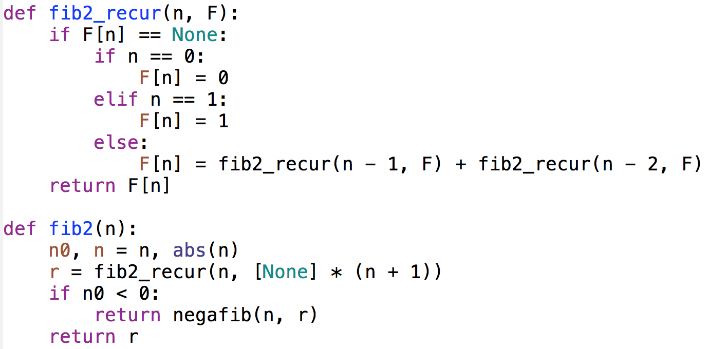
3.2 Algorithm fib2: Top-down Dynamic Programming with Memoization

fib2 is equivalent to fib1 with the main change being the so-called memoization. Memoization allows the caching of the already computed Fibonacci numbers so that fib2 does not have to revisit already visited parts of the call tree.

Memoization reduces the time and space complexities drastically; it leads to at most $n$ additions. With constant-time arithmetic, the time complexity is $O(n)$. The space complexity is also linear.

With non-constant time arithmetic, the additions range in time complexity from $A(\lg F_{2})$ to $A(\lg F_{n-1})$. The sum of these additions leads to the time complexity of $O(n^{2})$ in bit operations. The space complexity is also quadratic in the number of bits.

Regarding algorithmic concepts, fib2 illustrates recursion, top-down dynamic programming, and memoization.

Figure 8: fib3(n): An algorithm to compute the $n$th Fibonacci number $F_{n}$ iteratively in constant space.

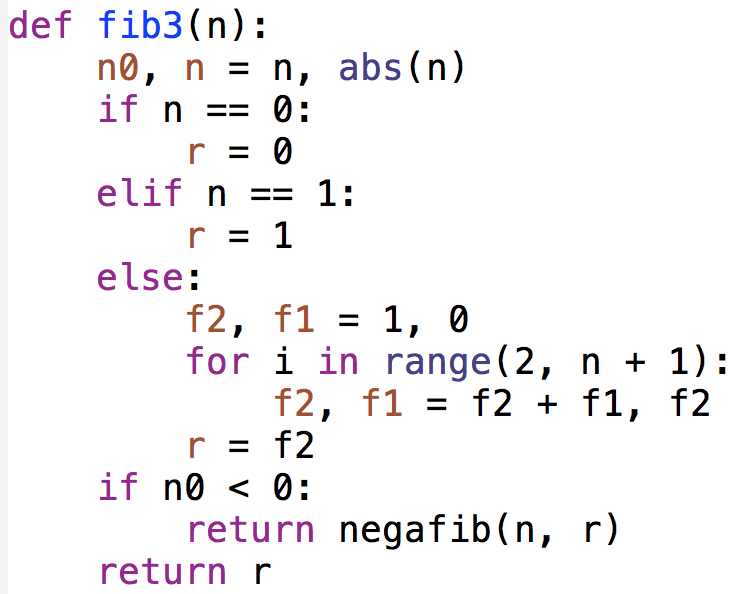
3.3 Algorithm fib3: Iteration with Constant Storage

fib3 uses the fact that each Fibonacci number depends only on the preceding two numbers in the Fibonacci sequence. This fact turns an algorithm designed top down, namely, fib2, to one designed bottom up. This fact also reduces the space usage to constant, just a few variables.

The time complexity is exactly the same as that of fib2. The space complexity is $O(1)$ with constant-time arithmetic and $O(n)$ with non-constant-time arithmetic.

Regarding the algorithmic concepts, fib3 illustrates iteration, recursion to iteration conversion, bottom-up dynamic programming, and constant space.

Figure 9: fib4(n): An algorithm to compute the $n$th Fibonacci number $F_{n}$ using a closed-form formula involving the golden ratio. The function num_pow_iter in the commented-out line may be used to instead of the library function math.pow.

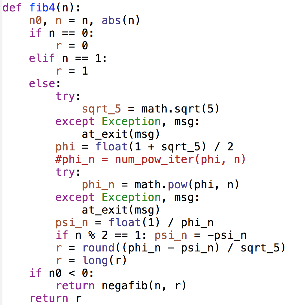
3.4 Algorithm fib4: Closed-form Formula with the Golden Ratio

fib4 uses the fact that the $n$th Fibonacci number has the following closed-form formula [7, 8]:

$$F_{n}=\left[\frac{\varphi^{n}-\psi^{n}}{\varphi-\psi}\right]=\left[\frac{\varphi^{n}-\psi^{n}}{\sqrt{5}}\right]$$ (3)

where

$$\varphi=\frac{1+\sqrt{5}}{2}\approx 1.618033$$ (4)

is the golden ratio,

$$\psi=\frac{1-\sqrt{5}}{2}=1-\psi=-\frac{1}{\varphi}\approx-0.618033$$ (5)

is the negative of its conjugate.

Note that to compute $\varphi^{n}$, this algorithm uses the standard math library function math.pow(phi,n) although num_pow_iter(phi,n) in the commented line can also be used.

This algorithm performs all its functions in floating-point arithmetic; the math functions in the algorithm map to machine instructions directly. Thus, this algorithm runs in constant time and space (also see [6] for an argument on non-constant time, assuming large $n$).

For $n>78$, this algorithm starts returning approximate results. For $n>1474$, this algorithm starts erroring out as $F_{n}$ is too large to even fit in a double precision floating point number width. These limits may change depending on the programming language and computer used but these general observations still hold.

Regarding the algorithmic concepts, fib4 illustrates the closed-form formula vs. iteration, integer vs. floating-point computation, and the exact vs. approximate result (or computation).

Figure 10: fib5(n): An algorithm to compute the $n$th Fibonacci number $F_{n}$ using a closed form equation using the golden ratio and rounding. The function num_pow_iter in the commented-out line may be used to instead of the library function math.pow.

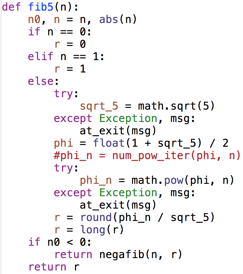
3.5 Algorithm fib5: Closed-form Formula with the Golden Ratio and Rounding

fib5 relies on the same closed-form formula used by fib4. However, it also uses the fact that $\psi$ is less than 1, meaning its $n$th power for large $n$ approaches zero [7, 8]. This means Eq. 3 reduces to

$$F_{n}=\left[{\frac{\varphi^{n}}{\sqrt{5}}}\right]$$ (6)

where $\varphi$ is the golden ratio.

For the same reasons as in fib4, this algorithm also runs in constant time and space.

The approximate behaviour of this algorithm is the same as that of fib4.

Regarding the algorithmic concepts, fib5 illustrates the concept of the optimization of a closed-form formula for speed-up in addition to the algorithmic concepts illustrated by fib4.

Figure 11: fib6(n): An algorithm to compute the $n$th Fibonacci number $F_{n}$ iteratively using the power of a certain 2x2 matrix. The function mat_mul may be used instead of its optimized version mat_mul_opt.

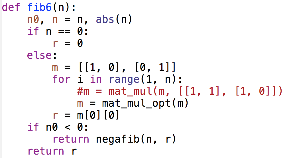
3.6 Algorithm fib6: The Power of a Certain 2x2 Matrix via Iteration

fib6 uses the power of a certain 2x2 matrix for the Fibonacci sequence [7, 8]:

$$\left(\begin{array}[]{cc}1&1\\ 1&0\end{array}\right)^{n-1}=\left(\begin{array}[]{cc}F_{n}&F_{n-1}\\ F_{n-1}&F_{n-2}\end{array}\right)$$ (7)

where $n\geq 2$. Then, $F_{n}$ is the largest element of the resulting 2x2 matrix.

The complexity analyses here are similar to those of fib2 or fib3. With constant-time arithmetic, the time complexity is $O(n)$. The space complexity in this case is also linear.

With non-constant time arithmetic, the additions range in time complexity from $A(\lg F_{1})$ to $A(\lg F_{n})$. The sum of these additions leads to the time complexity of $O(n^{2})$ in bit operations. The space complexity in this case is also quadratic in the number of bits.

Regarding the algorithmic concepts, fib6 illustrates (simple) matrix algebra and iteration over closed-form equations.

Figure 12: fib7(n): An algorithm to compute the $n$th Fibonacci number $F_{n}$ via repeated squaring recursively using the power of a certain 2x2 matrix.

Figure 13: fib8(n): An algorithm to compute the $n$th Fibonacci number $F_{n}$ via repeated squaring iteratively using the power of a certain 2x2 matrix.

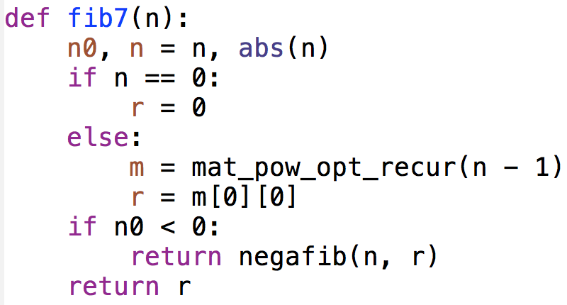
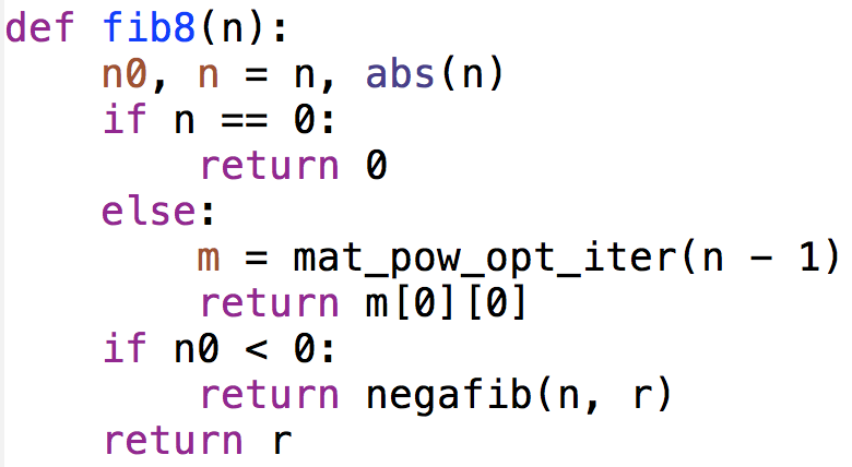
3.7 Algorithms fib7 and fib8: The Power of a Certain 2x2 Matrix via Repeated Squaring

fib7 and fib8 use the same equations used in fib6 but while fib6 uses iteration for exponentiation, fib7 and fib8 uses repeated squaring for speed-up. Moreover, fib7 uses a recursive version of repeated squaring while fib8 uses an iterative version of it.

Repeated squaring reduces time from linear to logarithmic. Hence, with constant time arithmetic, the time complexity is $O(\lg n)$. The space complexity is also logarithmic in $n$.

With non-constant time arithmetic, the additions range in time complexity from $A(\lg F_{1})$ to $A(\lg F_{n})$. The sum of these additions with repeated squaring leads to the time complexity of $O(n)$ in bit operations. The space complexity is also linear in the number of bits.

Regarding the algorithmic concepts, fib7 and fib8 illustrate (simple) matrix algebra, and repeated squaring over closed-form equations. In addition, fib7 illustrates recursion while fib8 illustrates iteration to perform repeated squaring over a matrix.

Figure 14: fib9(n): An algorithm to compute the $n$th Fibonacci number $F_{n}$ recursively using a certain recursive formula.

Figure 15: fib10(n): An algorithm to compute the $n$th Fibonacci number $F_{n}$ iteratively using a certain recursive formula.

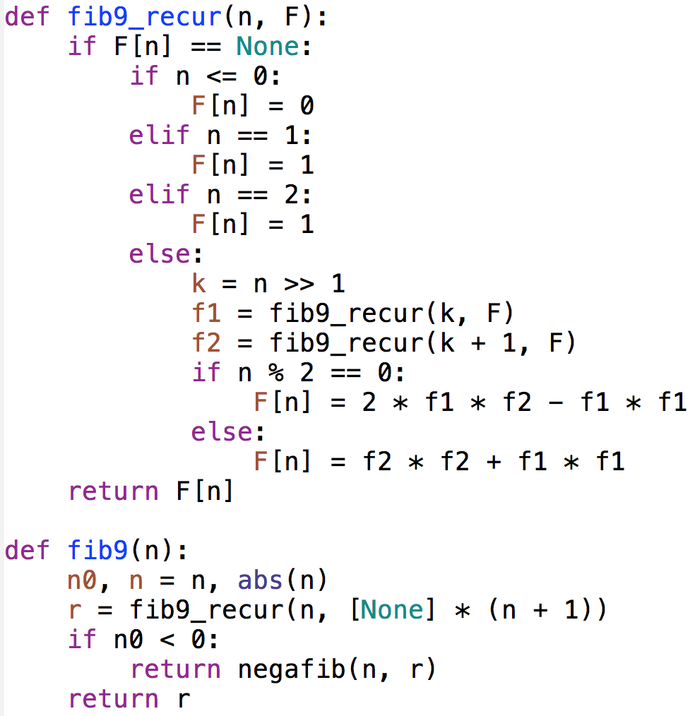
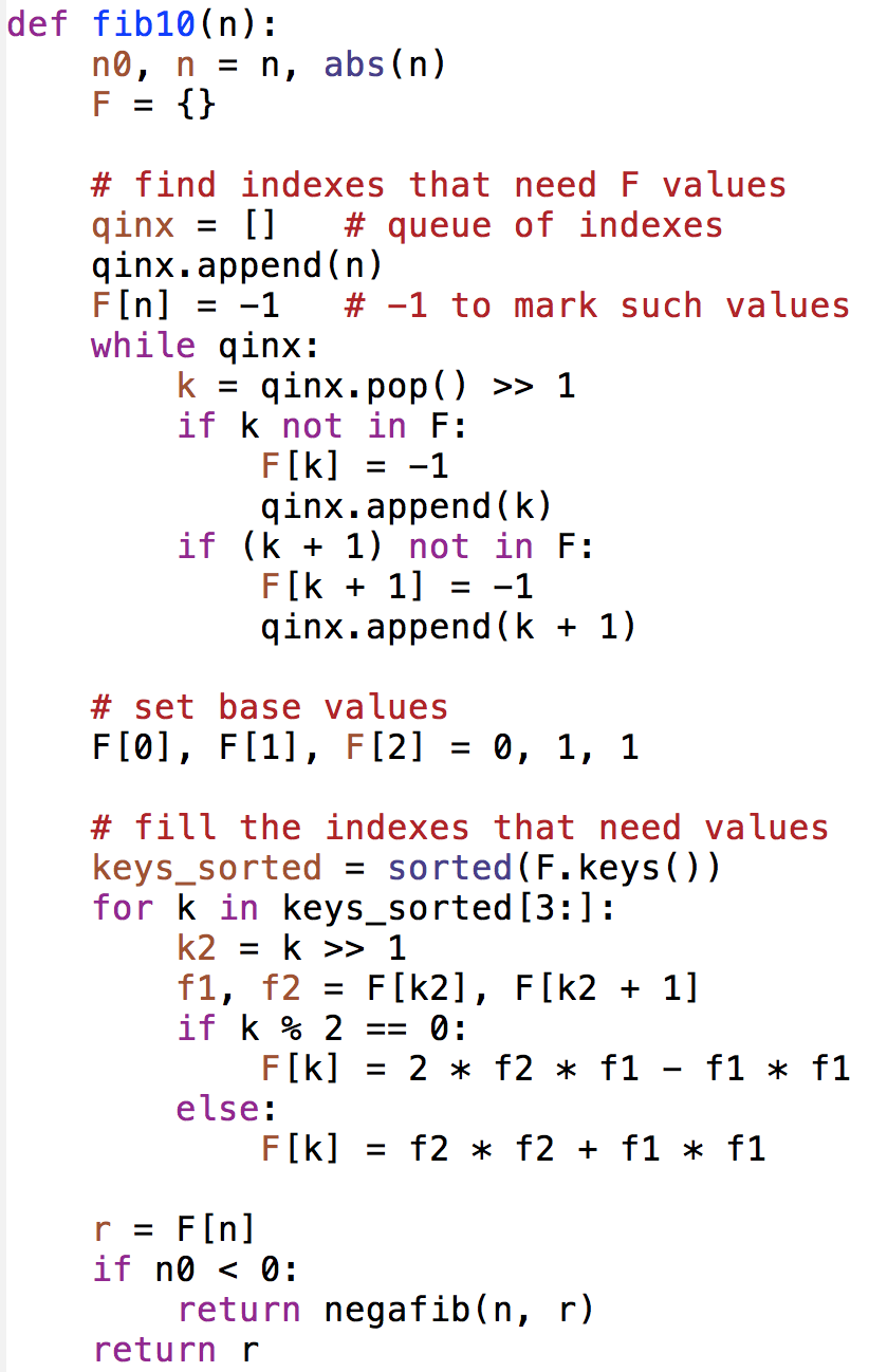
3.8 Algorithms fib9 and fib10: A Certain Recursive Formula

Both fib9 and fib10 use the following formulas for the Fibonacci sequence [8].

$$F_{2n+1}=F_{n+1}^{2}+F_{n}^{2}\mbox{ and }F_{2n}=2F_{n+1}F_{n}-F_{n}^{2}$$ (8)

where $n\geq 2$, with the base values $F_{2}=1$, $F_{1}=1$, and $F_{0}=0$. Note that memoization is used for speed-up in such a way that only the cells needed for the final result are filled in the memoization table $F$. In fib9, recursion takes care of identifying such cells. In fib10, a cell marking phase, using $F$ as a queue data structure, is used for such identification; then the values for these cells, starting from the base values, are computed in a bottom-up fashion.

These algorithms behave like repeated squaring in terms of time complexity. Hence, with constant time arithmetic, the time complexity is $O(\lg n)$. The space complexity is also logarithmic in $n$.

With non-constant time arithmetic, the additions range in time complexity from $A(\lg F_{1})$ to $A(\lg F_{n})$. The sum of these additions leads to the time complexity of $O(n)$ in bit operations. The space complexity is also linear in the number of bits.

Regarding the algorithm concepts, these algorithms illustrate recursion vs. iteration, top-down vs. bottom-up processing and/or dynamic programming, implementation of a recursive relation, and careful use of a queue data structure to eliminate unnecessary work in the bottom-up processing.

Figure 16: fib11(n): An algorithm to compute the $n$th Fibonacci number $F_{n}$ iteratively using a certain recursive formula.

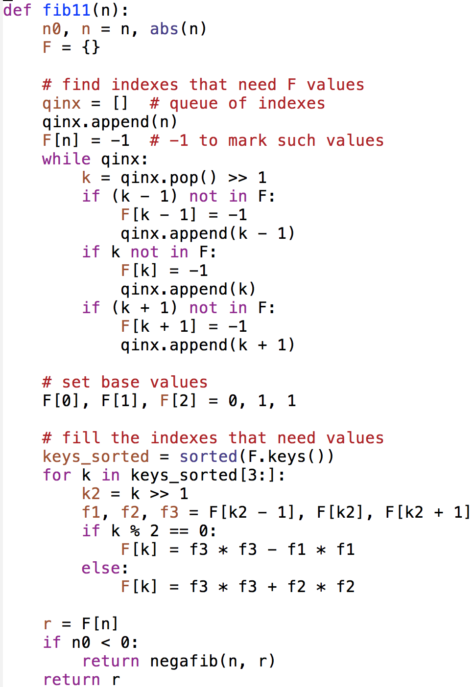
3.9 Algorithm fib11: Yet Another Recursive Formula

fib11 uses the following formulas for the Fibonacci sequence [8].

$$F_{2n+1}=F_{n+1}^{2}+F_{n}^{2}\mbox{ and }F_{2n}=F_{n}^{2}+2F_{n-1}F_{n}$$ (9)

where $n\geq 2$. The case for $n=2$ needs to be handled as a base case of recursion to prevent an infinite loop. Note that memoization is also used for speed-up.

The time and space complexity analyses are as in fib9 and fib10.

Regarding the algorithmic concepts, this algorithm is again similar to fib9 and fib10.

Figure 17: fib12(n): An algorithm to compute the $n$th Fibonacci number $F_{n}$ iteratively using a certain recursive formula.

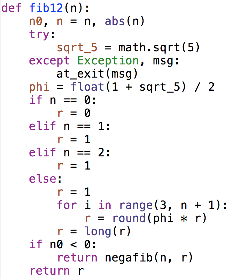
3.10 Algorithm fib12: Yet Another but Simpler Recursive Formula

fib12 uses the following formula for the Fibonacci sequence

$$F_{n}=\left[\varphi F_{n-1}\right]$$ (10)

where $n\geq 3$. We could not find a specific reference in the literature for this formula even though it seems derivable from Eq. 3 and the fact that the golden ratio is the limit value that the ratio $\frac{F_{n}}{F_{n-1}}$ approaches as $n$ gets larger.

Note that although the golden ratio is the limit value of the ratio of the consecutive Fibonacci numbers, this algorithm shows that even for small values $n$, from 3 to 78 to be exact, $F_{n}=[\varphi F_{n-1}]$, where the round operation seems to make this formula work. For larger $n$, this algorithm, like the algorithms fib4 and fib5, return approximate results due to the use of floating-point arithmetic.

The time and space complexity analyses are as in fib3. It is easy to implement a version of this algorithm where both recursion and memoization are used.

Regarding the algorithmic concepts, this algorithm illustrates the iterative version of a recursive formula.

4 Results

We now present the results of a small-scale experimental analysis done on a high-end laptop computer (model: MacBook Pro, operating system: macOS Sierra 10.12.6, CPU: 2.5 GHz Intel Core i7, main memory: 16GB 1600 MHz DDR3).

For each algorithm, we measure its runtime in seconds (using the clock() method from the time module in the Python standard library). We ran each algorithm 10,000 times and collected the runtimes. The reported runtimes are the averages over these repetitions. We also computed the standard deviation over these runtimes. We use the standard deviation to report “the coefficient of variability” (CV) (the ratio of the standard deviation to the average runtime of an algorithm over 10,000 repetitions), which gives an idea on the variability of the runtimes.

We report the results in four groups, moving the focus towards the fastest algorithms as $n$ gets larger:

1. The case $0\leq n\leq 30$ is small enough to run all algorithms, including the slowest algorithm fib1.

2. The case $0\leq n\leq 70$ excludes the slowest algorithm fib1. In this case all algorithms are exact. On our experimental setting, the algorithms fib4, fib5, and fib12 start returning approximate results after 70 (78 to be exact on our setting).

3. The case $0\leq n\leq 900$ excludes the approximation algorithms, i.e., fib4, fib5, and fib12. The upper bound $900$ is also roughly the upper bound beyond which the recursive algorithms start exceeding their maximum recursion depth limit and error out.

4. The case $0\leq n\leq 10,000$ focuses on the fastest algorithms only, excluding the slow algorithms, the recursive algorithms, and the approximate algorithms.

Each plot in the sequel has two axes: The x-axis is $n$, as in the index of $F_{n}$; and the y-axis is the average runtime in seconds over 10,000 repetitions.

To rank the algorithms in runtime, we use the sum of all the runtimes across all the $n$ range. These rankings should be taken as directionally correct as the variability in runtimes, especially for small $n$, makes it difficult to assert a definite ranking.

Table 1: Algorithms

	Runtime in	Runtime in
Algorithm	constant-time ops	bit ops
fib1	$O(\varphi^{n})$	$O(\varphi^{n})$
fib2	$O(n)$	$O(n^{2})$
fib3	$O(n)$	$O(n^{2})$
fib4	$O(1)$	$O(1)$
fib5	$O(1)$	$O(1)$
fib6	$O(n)$	$O(n^{2})$
fib7	$O(\lg n)$	$O(n)$
fib8	$O(\lg n)$	$O(n)$
fib9	$O(\lg n)$	$O(n)$
fib10	$O(\lg n)$	$O(n)$
fib11	$O(\lg n)$	$O(n)$
fib12	$O(n)$	$O(n^{2})$

Figure 18: Results until fib1 takes too much time.

Figure 19: Coefficient of variation for above.

4.1 Results with all algorithms

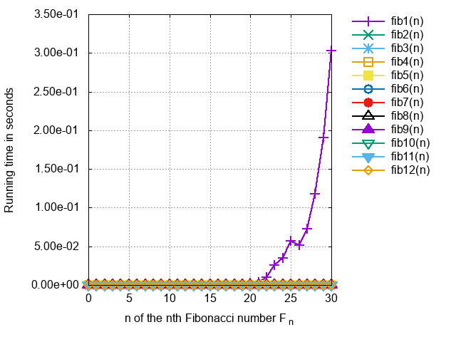
The results with $0\leq n\leq 30$ in Fig. 18 mainly show that the exponential-time algorithm fib1 significantly dominates all others in runtime. This algorithm is not practical at all to use for larger $n$ to compute the Fibonacci numbers. The ratio of the slowest runtime to the fastest runtime, that of fib5, is about four orders of magnitude, 14,000 to be exact on our experimental setting.

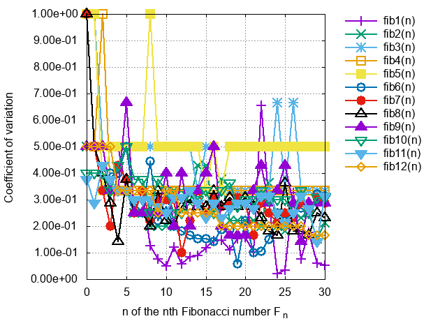
The CV results in Fig. 19 do not seem very reliable since the runtimes are very small. Yet the CV results largely fall roughly below 35% with an outlier at 50% for fib5. For the slowest algorithm fib1, the CV is largely around 5%, which is expected given its relatively large runtime.

Figure 20: Results with all algorithms (excl. fib1) returning exact results.

Figure 21: Coefficient of variation for above.

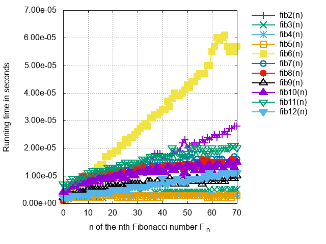
4.2 Results with all fast algorithms returning exact results

The results with $0\leq n\leq 70$ in Fig. 20 excludes the slowest algorithm fib1. The results show that fib6 is now the slowest among the rest of the algorithms; its runtime seems to grow linearly with $n$ while the runtimes of the rest of the algorithms seem to grow sublinearly. The algorithms implementing the closed-form formulas seem to run in almost constant time.

The algorithms group as follows in terms of their runtimes in increasing runtime order:

• fib5, fib4, fib3;

• fib12, fib9;

• fib10, fib8, fib7, fib2, fib11;

• fib6.

These runtimes show that the algorithms implementing the closed-form formulas are the fastest. The ratio of the slowest runtime, that of fib6, to the fastest runtime, that of fib5, is about an order of magnitude, 13 to be exact on our experimental setting.

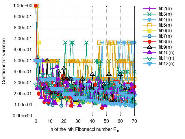
The CV results in Fig. 21 are similar to the case for the first case above.

Figure 22: Results until recursive algorithms hit too deep a recursion depth.

Figure 23: Coefficient of variation for above.

Figure 24: Results until recursive algorithms hit too deep a recursion depth. Faster algorithms focus.

Figure 25: Results until recursive algorithms hit too deep a recursion depth. Even faster algorithms focus.

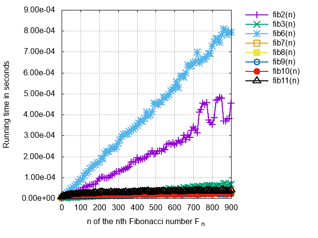
4.3 Results within safe recursion depth

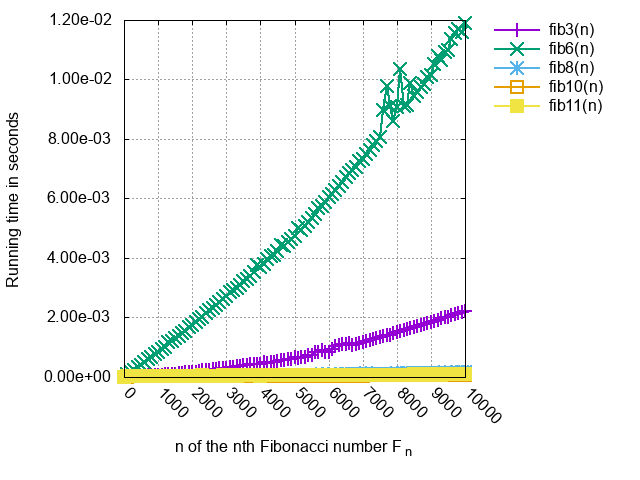
The results with $0\leq n\leq 900$ in Fig. 22 excludes the slowest algorithm fib1. The upper bound of $n$ is roughly the limit beyond which recursive algorithms fail due to the violation of their maximum recursion depth.

The results show that fib6 followed by fib2 are the slowest among the rest of the algorithms; their runtimes seem to grow linearly with $n$ but the slope for fib2 is significantly smaller. The algorithms grow sublinearly in terms of their runtimes. Again, the algorithms implementing the closed-form formulas seem to run in almost constant time.

The algorithms group as follows in terms of their runtimes in increasing runtime order:

• fib5, fib4;

• fib9, fib10, fib8, fib7, fib11, fib3;

• fib12;

• fib2;

• fib6.

The ratio of the slowest runtime, that of fib6, to the fastest runtime, that of fib5, is about two orders of magnitude, 152 to be exact on our experimental setting.

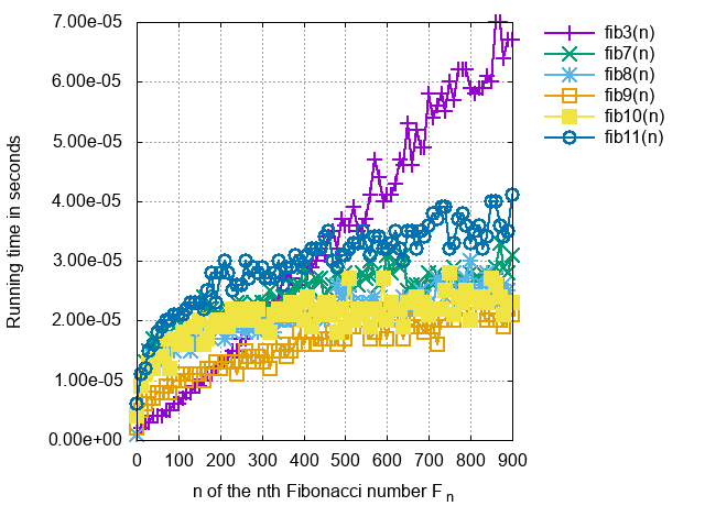
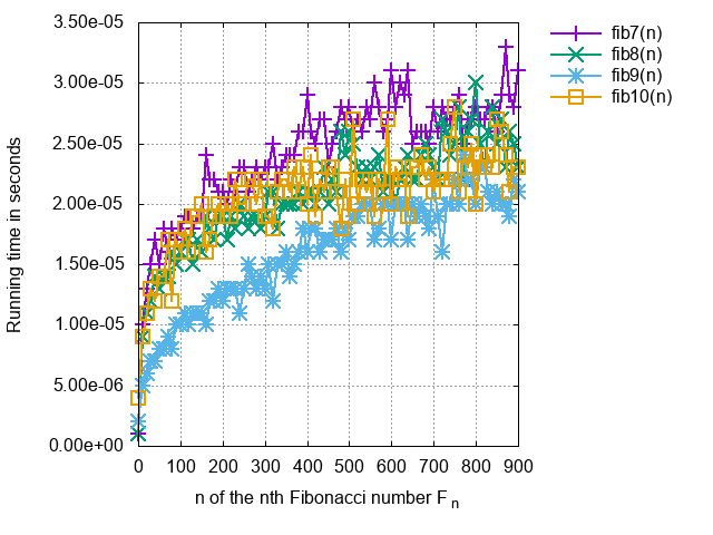
Fig. 24 and Fig. 25 zoom in on the faster algorithms, excluding the slowest algorithms from Fig. 22.

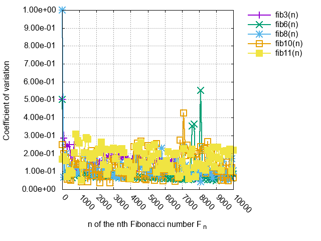
The CV results in Fig. 23 all seem to be below 20%, which seems reasonably small given that the runtimes are now larger.

Figure 26: Results using only iterative algorithms with exact results.

Figure 27: Coefficient of variation for above.

Figure 28: Results using only iterative algorithms with exact results. Faster algorithms focus.

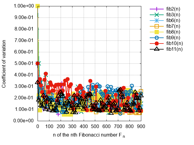
4.4 Results with the fastest iterative and exact algorithms

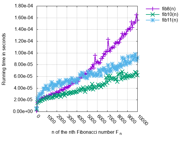
The results with $0\leq n\leq 10k$ in Fig. 26 excludes all slow algorithms, all recursive algorithms, and all inexact algorithms, those that do not return exact results.

In this range where $n$ gets very large, the fastest and slowest algorithms are fib10 and fib6, respectively. The algorithms group as follows in terms of their runtimes in increasing runtime order:

• fib10, fib8, fib11;

• fib3;

• fib6.

The ratio of the slowest runtime, that of fib6, to the fastest runtime, that of fib10, is about two orders of magnitude, 130 to be exact on our experimental setting.

Fig. 24 zooms in on the fastest algorithms, excluding the slowest algorithms from Fig. 26.

The CV results in Fig. 27 all seem to have converged to values below 20%, which again seems reasonably small given that the runtimes are now larger with such large $n$.

5 Conclusions

The Fibonacci numbers are well known and simple to understand. We have selected from the technical literature [1, 5, 7, 8] twelve methods of computing these numbers. Some of these methods are recursive formulas and some others are closed-form formulas. We have translated each method to an algorithm and implemented in the Python programming language. Each algorithm takes in $n$ to return the $n$ Fibonacci number $F_{n}$.

Though simple, these algorithms illustrate a surprisingly large number of concepts from the algorithms field: Top-down vs. bottom-up dynamic programming, dynamic programming with vs. without memoization, recursion vs. iteration, integer vs. floating-point arithmetic, exact vs approximate results, exponential- vs. polynomial-time, constant-time vs non-constant-time arithmetic, constant to polynomial to exponential time and space complexity, closed-form vs. recursive formulas, repeated squaring vs. linear iteration for exponentiation, recursion depth and probably more. The simplicity of these algorithms then becomes a valuable asset in teaching introductory algorithms to students in that students can focus on these concepts rather than the complexity of the algorithms.

We have also presented a small-scale experimental analysis of these algorithms to further enhance their understanding. The analysis reveals a couple of interesting observations, e.g., how two algorithms that implementing seemingly similar recursive formulas may have widely different runtimes, how space usage can affect time, how or why recursive algorithms cannot have too many recursive calls, when approximate algorithms stop returning exact results, etc. The results section explain these observations in detail with plots.

Probably the simplest and fast algorithm to implement is fib3, the one that uses constant space. However, the fastest algorithm, especially for large $n$, turns out to be fib10, the one that implements a recursive algorithm with a logarithmic number of iterations. When $n\leq 70$ where all algorithms return exact results, the fastest algorithms are fib4 and fib5, the ones that implement the closed-form formulas.

The slowest algorithm is of course fib1, the one that implements probably the most well-known recursive formula, which is usually also the definition of the Fibonacci numbers. Memoization does speed it up immensely but there is no need to add complexity when simpler and faster algorithms also exist.

We hope that this paper can serve as a useful resource for students learning and teachers teaching the basics of algorithms. All the programs used for this study are at [2].

6 Homework Questions

We now list a couple of homework questions for the students. These questions should help improve the students’ understanding of the algorithmic concepts further.

1. Try to simplify the algorithms further, if possible.

2. Try to optimize the algorithms further, if possible.

3. Replace $O$ to $\Theta$ in the complexity analyses, if possible.

4. Prove the time and space complexities for each algorithm.

5. Improve, if possible, the time and space complexities for each algorithm. A trivial way is to use the improved bounds on $M(\cdot)$.

6. Reimplement the algorithms in other programming languages. The simplicity of these algorithms should help in the speed of implementing in another programming language.

7. Derive an empirical expression for the runtime of each algorithm. This can help derive the constants hidden in the $O$-notation (specific to a particular compute setup).

8. Rank the algorithms in terms of runtime using statistically more robust methods than what this paper uses.

9. Find statistically more robust methods to measure the variability in the runtimes and/or to bound the runtimes.

10. Explain the reasons for observing different real runtimes for the algorithms that have the same asymptotic time complexity.

11. Learn more about the concepts related to recursion such as call stack, recursion depth, and tail recursion. What happens if there is no bound on the recursion depth?

12. Explain in detail how each algorithm illustrates the algorithmic concepts that this paper claims it does.

13. Design and implement a recursive version of the algorithm fib11.

14. Design and implement versions of the algorithms fib4 and fib5 that use rational arithmetic rather than floating-point arithmetic. For the non-rational real numbers, use their best rational approximation to approximate them using rational numbers at different denominator magnitudes.

15. Find other formulas for the Fibonacci numbers and implement them as algorithms.

16. Prove the formula used by the algorithm fib12.

17. Use the formula involving binomial coefficients to compute the Fibonacci numbers. This will also help teach the many ways of computing binomial coefficients.

18. Design and implement multi-threaded or parallelized versions of each algorithm. Find out which algorithm is the easiest to parallelize and which algorithm runs faster when parallelized.

19. Responsibly update Wikipedia using the learnings from this study and/or your extensions of this study.

References

- [1] T. Cormen, C. S. R. Rivest, and C. Leiserson. Introduction to Algorithms. McGraw-Hill Higher Education, 2nd edition, 2001.
- [2] A. Dasdan. Fibonacci Number Algorithms. https://github.com/alidasdan/fibonacci-number-algorithms.
- [3] M.Forišek. Towards a Better Way to Teach Dynamic Programming. Olympiads in Informatics. vol. 9. 2015.
- [4] D.Goldberg. What Every Computer Scientist Should Know About Floating-Point Arithmetic. ACM Computing Surveys, Vol 23(1), 5–48, 1991.
- [5] R. L. Graham, D. E. Knuth, and O. Patashnik. Concrete Mathematics: A Foundation for Computer Science. Addison-Wesley, 2nd edition, 1994.
- [6] J. L. Holloway. Algorithms for Computing Fibonacci Numbers Quickly. MSc Thesis. Oregon State Univ. 1988.
- [7] J. Sondow and E. Weisstein. Fibonacci number. In From MathWorld–A Wolfram Web Resource. Wolfram. Referenced in Jan 2018. http://mathworld.wolfram.com/FibonacciNumber.html.
- [8] Wikipedia. Fibonacci number. Referenced in Jan 2018. https://en.wikipedia.org/wiki/Fibonacci_number.
- [9] Wikipedia. Computational complexity of mathematical operations. Referenced in Mar 2018. https://en.wikipedia.org/wiki/Computational_complexity_of_mathematical_operations.
- [10] Wikipedia. Dynamic programming. Referenced in May 2018. https://en.wikipedia.org/wiki/Dynamic_programming.
- [11] Wikipedia. Recursion. Referenced in May 2018. https://en.wikipedia.org/wiki/Recursion_(computer_science).
- [12] Wikipedia. Time complexity. Referenced in May 2018. https://en.wikipedia.org/wiki/Time_complexity.
- [13] Wikipedia. Call Stack. Referenced in May 2018. https://en.wikipedia.org/wiki/Call_stack.
- [14] Wikipedia. Tail call. Referenced in May 2018. https://en.wikipedia.org/wiki/Tail_call.
- [15] Wikipedia. Floating-point arithmetic. Referenced in May 2018. https://en.wikipedia.org/wiki/Floating-point_arithmetic.
- [16] Wikipedia. Closed-form expression. Referenced in May 2018. https://en.wikipedia.org/wiki/Closed-form_expression