Consequences of Giant Impacts on Early Uranus for
Rotation, Internal Structure, Debris, and Atmospheric Erosion

Abstract

We perform a suite of smoothed particle hydrodynamics simulations to investigate in detail the results of a giant impact on the young Uranus. We study the internal structure, rotation rate, and atmospheric retention of the post-impact planet, as well as the composition of material ejected into orbit. Most of the material from the impactor’s rocky core falls in to the core of the target. However, for higher angular momentum impacts, significant amounts become embedded anisotropically as lumps in the ice layer. Furthermore, most of the impactor’s ice and energy is deposited in a hot, high-entropy shell at a radius of $\sim$3 $R_{\oplus}$. This could explain Uranus’ observed lack of heat flow from the interior and be relevant for understanding its asymmetric magnetic field. We verify the results from the single previous study of lower resolution simulations that an impactor with a mass of at least 2 $M_{\oplus}$ can produce sufficiently rapid rotation in the post-impact Uranus for a range of angular momenta. At least 90% of the atmosphere remains bound to the final planet after the collision, but over half can be ejected beyond the Roche radius by a 2 or 3 $M_{\oplus}$ impactor. This atmospheric erosion peaks for intermediate impactor angular momenta ($\sim$$3\times 10^{36}$ kg m² s^-1). Rock is more efficiently placed into orbit and made available for satellite formation by 2 $M_{\oplus}$ impactors than 3 $M_{\oplus}$ ones, because it requires tidal disruption that is suppressed by the more massive impactors.

1 Introduction

Uranus spins on its side. With an obliquity of 98^∘ and its major moons orbiting in the same tilted plane, the common explanation is that a giant impact sent the young Uranus spinning in this new direction (Safronov, 1966). This impact might also help explain other phenomena, such as the striking differences between Uranus’ and Neptune’s satellite systems (Morbidelli et al., 2012; Parisi et al., 2008), the remarkable lack of heat from Uranus’ interior (Stevenson, 1986; Podolak & Helled, 2012; Nettelmann et al., 2016), and its highly asymmetrical and off-axis magnetic field (Ness et al., 1986). Until now, this violent event itself has been little studied since the first smoothed particle hydrodynamics (SPH) simulations of Slattery et al. (1992).

Uranus’ equatorial ring and satellite system is remarkable in several respects. It features a set of regular, prograde, major moons, a compact inner system of rings and small satellites, and a distant group of irregular moons. The inner system and major moons are hypothesised to have formed either from a post-impact debris disk (Stevenson, 1986; Slattery et al., 1992) or from a pre-impact proto-satellite disk that was destabilised by the post-impact debris disk and rotated to become equatorial (Morbidelli et al., 2012; Canup & Ward, 2006). The more-distant irregular satellites are thought to have been captured after the impact (Parisi et al., 2008).

The interior structure of Uranus is poorly understood. Surface emission is in approximate equilibrium with solar insolation, implying that negligible heat flows out from the planet, in striking contrast with the other giant planets (Pearl et al., 1990). This might be explained by restricted interior convection, perhaps caused by the deposition of the impactor’s energy into a thin shell (Stevenson, 1986; Podolak & Helled, 2012). Such a thermal boundary layer between an outer H–He-rich envelope and an inner ice-rich layer was the crucial ingredient for the evolutionary model of Uranus produced by Nettelmann et al. (2016) that was consistent with both heat flow and gravitational moment measurements.

In contrast with terrestrial planets, the magnetic field of Uranus measured by Voyager 2 was not dominated by the dipole component. Higher order moments contributed significantly, and the dipole itself was both offset by approximately 0.3 Uranus radii from the centre of the planet and tilted by $60^{\circ}$ relative to Uranus’ rotation axis (Ness et al., 1986). Dynamo models producing similar magnetic fields have been constructed using a layer of convecting electrically conducting ices (Stanley & Bloxham, 2004, 2006; Soderlund et al., 2013). A feature of some of these models is the presence of a stably stratified fluid layer interior to the zone where the magnetic field is generated.

As a separate source of motivation, while the ice giants Uranus and Neptune do not receive as much attention as the nearer bodies in the solar system, they represent the closest analogues to the mini-Neptune-class exoplanets that are the most frequently discovered by Kepler (Batalha, 2014). Given the detection efficiencies, these planets are typically found on orbits with periods of the order of 100 days (Fressin et al., 2013), but have nevertheless stimulated attempts to understand the atmospheres and histories of our ice giants in order to provide context for these exoplanet observations (Fortney et al., 2013).

The first simulations of a giant impact onto a proto-Uranus, albeit in one dimension, were done specifically to investigate whether the shock from the collision would blast away Uranus’ hydrogen–helium atmosphere (Korycansky et al., 1990). This gas has a much lower mass fraction and density than the inner ice and rock material, so requires high resolution to simulate. For this reason, Korycansky et al. (1990) restricted their study to a one-dimensional spherically symmetric model where the impactor mass and some of its energy was injected into the proto-Uranus core, and the remaining energy was placed into the atmosphere. The retained atmospheric mass was found to depend sensitively upon the amount of energy deposited directly into the atmosphere, offering the possibility that the presence of Uranus’ current atmosphere might constrain allowable impact scenarios.

Building on the pioneering work of Benz et al. (1986), who used SPH simulations to model the Moon-forming giant impact on the Earth, Slattery et al. (1992) (hereafter S92) produced, to our knowledge, the only paper to date with three-dimensional hydrodynamical simulations of the hypothesised impact event that befell the proto-Uranus. While the $<$$10^{4}$-particle SPH simulations of S92 did not resolve the atmosphere, they studied collisions between a 1 and 3 $M_{\oplus}$ differentiated impactor containing iron, dunite, and ice and a similarly differentiated proto-Uranus with hydrogen and helium mixed into its ice layer. For impactor masses above 1 $M_{\oplus}$, they found a wide range of impact scenarios that led to a sufficiently rapidly spinning planet. Most of these collisions left ice in orbit, but only the higher angular momentum ones also placed any rock or iron into orbit, as might be expected if this material is subsequently to form any of the currently observed regular moons. Uranus’ satellites comprise only $\sim$10^-4 of the total system mass—the same mass fraction as the other giant planets—corresponding to just less than the mass of a single particle in S92’s simulations.

In this paper, we present new simulations of the impact with orders of magnitude better mass resolutions than those of S92, allowing the detailed modelling of, for example, Uranus’ atmosphere and its fate; the deposition of the impactor’s material and energy inside Uranus; the post-impact debris disk, in particular the amount, distribution, and composition of material available for satellite formation; and the testing of S92’s original conclusions for the types of impacts that could have produced the present-day spin.

Section 2 describes the methods used to construct initial conditions and run the impact simulations. Our results are reported and discussed in section 3, and the findings are summarised in section 4.

2 Methods

In this section, we first outline the equations of state (EoS) used for the various materials in the simulations and the generation of the initial conditions, followed by detailing the simulation runs themselves.

2.1 EoS and Initial Conditions

Planets contain multiple and complex materials, so a few different EoS—which relate the pressure, density, and temperature or specific internal energy—need to be specified for our SPH simulations.

Our proto-Uranus contains a rocky core (SiO₂, MgO, FeS, and FeO), icy mantle (H₂O, NH₃, and CH₄), and atmosphere with a solar composition mix of hydrogen and helium. These materials were used for the Uranus model of Hubbard & MacFarlane (1980) (hereafter HM80), and for our simulations described here we use the EoS as presented in their paper (appendix A). These relatively straightforward EoS provide us with some baseline simulation results that will in the future be compared with more advanced EoS, such as those more recently determined for ices and hydrogen and helium (Nettelmann et al., 2008; Redmer et al., 2011; Militzer & Hubbard, 2013; Bethkenhagen et al., 2013; Wilson et al., 2013; Bethkenhagen et al., 2017).

We use a range of impactor masses of $M_{\rm{i}}=1$, 2, and 3 $M_{\oplus}$ and, under the assumption that little mass escapes during the impact, set the mass of the proto-Uranus to be 14.536 $M_{\oplus}-M_{\rm{i}}$. The proto-Uranus is differentiated into the three distinct layers described above. The impactor is given no atmosphere, so it has only a rocky core surrounded by an icy mantle, with the ice/rock mass ratio matching that in the proto-Uranus.

To determine the amounts of rock, ice, and atmosphere in the two bodies, we first create a spherically symmetric three-layer model for the present-day Uranus, assuming hydrostatic equilibrium. The assumed outer boundary conditions are a pressure of 1 bar and a temperature of 60 K at a radius of 3.98 $R_{\oplus}$. We then iterate the radii of the layer boundaries until the profile contains the desired total mass (14.536 $M_{\oplus}$) and a reduced moment of inertia of $I/(MR^{2})=0.21$. The outer temperature is slightly lower than the measured value (75 K), in order that this simple model can approach the observed reduced moment of inertia of 0.22 (Podolak & Helled, 2012). We find an ice-rich body, with 2.02, 11.68, and 0.84 $M_{\oplus}$ in the rock, ice, and atmosphere layers, respectively, with inner boundaries at radii of 1.0 and 3.1 $R_{\oplus}$. There is considerable uncertainty in the composition of Uranus; this ratio of ice to rock is comparable with that in the model of Nettelmann et al. (2013), but larger than that found by HM80 and almost twice the solar system value adopted by S92.

The density, temperature, and pressure profiles for our Uranus model as well as the three proto-Uranus and impactor pairs are shown in Figure 1. Also included are the density–temperature relations, showing our isothermal rocky cores, the approximately adiabatic power-law relation for the ice mixture used by HM80, and their fitted polynomial adiabat for the atmosphere.

One simplification present in our initial conditions is the lack of compositional mixing between the different layers. For instance, S92 included H–He mixed into the icy mantle of their proto-Uranus, and the model of Hubbard & Marley (1989) had some ice mixed into the rocky core. Given the uncertainties in the current internal structure of Uranus, and the much larger uncertainties in those of the proto-Uranus and impactor, we opt for simply differentiated bodies for these initial investigations.

The impacts we consider are violent enough to dominate over any pre-existing rotation, so our proto-Uranus (and impactor) begins without any spin. This spherical symmetry also makes the generation of initial conditions much simpler, so we leave investigating the effects of pre-impact spin for a future study.

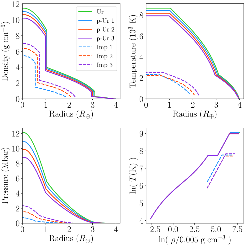
Figure 1: The density, temperature, and pressure profiles of our Uranus (Ur) model and the three pairs of proto-Uranus (p-Ur) and impactor (Imp) bodies. The bottom-right panel shows the temperature–density relations assumed in the various objects. The colours correspond to different masses of the impactor as labelled in the legend (in units of $M_{\oplus}$). The green line shows the model Uranus whose mass we split into the proto-Uranus and impactor.

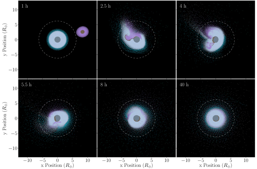
Figure 2: Snapshots from a low angular momentum impact simulation with a 2 $M_{\oplus}$ impactor and $L=2\times 10^{36}$ kg m² s^-1. Particles between $z=0$ and $-13$ $R_{\oplus}$ are shown, coloured by material type and originating body. Light and dark grey show the target’s ice and rock material, respectively, and purple and brown show the same for the impactor. Light blue is the target’s atmosphere. The white dashed circle traces out the current Roche radius of Uranus for reference. The snapshot times are given to the nearest half hour since the start of the simulation. This figure is available as an animation in the online version.

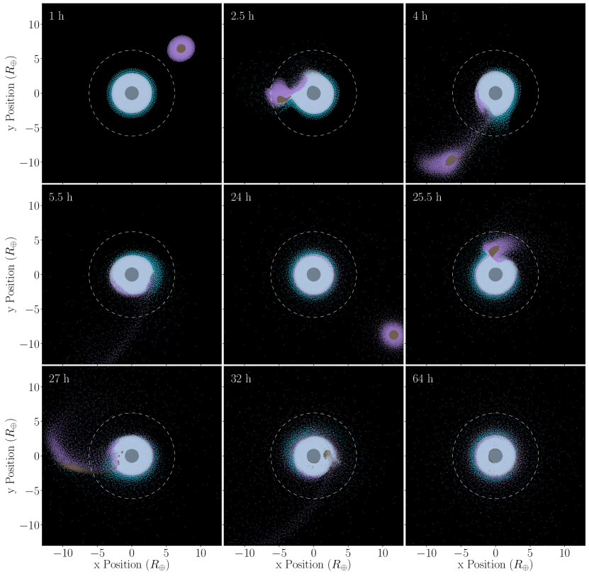
Figure 3: As for Figure 2, but for a high angular momentum impact simulation with a 2 $M_{\oplus}$ impactor and $L=5\times 10^{36}$ kg m² s^-1. This figure is available as an animation in the online version.

2.2 Particle Placement

The EoS for the ice and rock materials being simulated are very stiff, i.e. a small variation in density changes the pressure dramatically. It is therefore important to reduce particle noise when sampling the desired mass distribution with particles. Even small deviations from the profile density will lead to transient behaviour that can take a long time to settle, during which the particle distribution may also significantly change.

We have developed a new algorithm for quickly creating low-noise particle distributions for an arbitrary spherically symmetric mass distribution, such that every particle’s SPH density is within 1% of the desired value (Kegerreis et al., 2018, in prep.). The code is publicly available at https://github.com/jkeger/seagen and the seagen python module can be installed directly with pip.

Raskin & Owen (2016) and Reinhardt and Stadel (2017) developed comparable approaches to the challenge of placing particles to represent spherically symmetric mass distributions in ways that avoided the various problems of lattice-based methods (Herant, 1994). However, we found that the method of Raskin & Owen (2016) leads to a few particles in every shell having significant overdensities, causing unrealistically high pressures with the stiff EoS. The approach of Reinhardt and Stadel (2017) cannot place arbitrary numbers of particles in each shell. Consequently, some particles show SPH densities more than 5% discrepant from the profile.

Our method leads to initial conditions that are close to equilibrium and quick to produce, avoiding the need for a lengthy simulation to relax the system. Briefly, our method involves distributing any arbitrary number of particles in spherical shells (a nontrivial problem (Saff & Kuijlaars, 1997)), starting by dividing a spherical shell into equal-area regions arranged into iso-latitude bands. An empirical stretch away from the poles is then applied so that the particles, when placed in the centres of these regions, all have very similar densities as determined using the relevant SPH smoothing kernel. All particles have a similar mass, with mass variations of $\sim$3% because of the integer numbers in each shell. Concentric shells can then be set up to follow precisely an arbitrary radial density profile with very low scatter in each shell.

The small density discrepancies in this particle placement scheme result in average transient particle speeds in our initial conditions that are already under 1% of the escape speed. A quick relaxation simulation, described in section 2.3, further reduces this by an order of magnitude.

2.3 SPH Simulations

All simulations were run with a version of the parallel tree-code HOT (Warren & Salmon, 1993) that has been modified to include SPH (Lucy, 1977; Gingold & Monaghan, 1977) and the relevant EoS described in section 2.1 (see also appendix A). The SPH formulation is described in Fryer et al. (2006). Particles with different EoS are adjacent at the boundaries, which can cause problems in SPH given the sharp density changes, in addition to the known issues regarding the mixing of materials (Woolfson, 2007; Hosono et al., 2016; Deng et al., 2017). To verify the stability of our model planets given the lack of any special boundary treatments in this simple SPH formulation, we ran a simulation where the impactor misses the target but is slightly tidally disrupted, so that any problems would not be hidden in the middle of a violent impact. We confirmed that the pressure at the core-mantle boundary evolved smoothly and remained stable, showing the same ‘unloading’ behaviour tested by Asphaug et al. (2006, Fig. 2(b)).

Initial simulations of the proto-Uranus and impactor for 10,000 s in isolation were performed including a damping force to further reduce any remaining small fluctuations in density. At the end of these simulations, the total kinetic energy was decreased from a fraction of $\sim$$10^{-5}$ to below $10^{-6}$ of the total energy. This corresponds to reducing the maximum particle velocity to below 1% of the target planet’s escape speed, with an average random velocity of $\sim$0.1% of the escape speed.

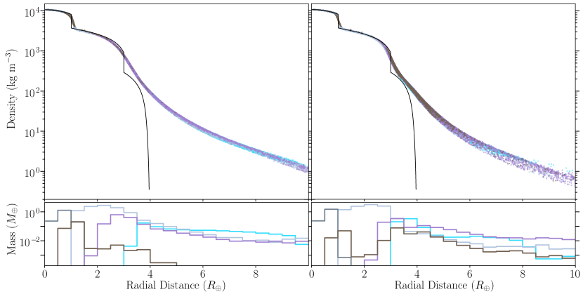
Figure 4: The final radial density profiles for the same relatively head-on (left) and grazing (right) impacts as in Figures 2 and 3. The black line shows the proto-Uranus density profile. The lower panels show the mass of particles in radial bins of width 0.5 $R_{\oplus}$, split by material type and originating body. Light and dark grey show the target’s ice and rock material, respectively, and purple and brown show the same for the impactor. Light blue is the target’s atmosphere.

Prior to impact, the impactor and proto-Uranus both become distorted by the gravitational tides from the other object. The subsequent evolution can depend significantly upon these departures from sphericity at impact. Thus, for an accurate reproduction of the collision, it is necessary to start the impactor sufficiently far enough away that these tidal distortions are faithfully followed. To achieve this, we placed the impactor such that its closest particle to the proto-Uranus received a 10 times larger gravitational force from the rest of the impactor than from the proto-Uranus. This amounts to separations of $\sim$22, 16, and 14 $R_{\oplus}$ for the 1, 2, and 3 $M_{\oplus}$ impactors respectively (appendix B).

Separate suites of impacts were created with just over $10^{5}$ and $10^{6}$ particles to test the resolution-dependence of our results. The angular momenta of the systems ranged from 1 to $10\times 10^{36}$ kg m² s^-1. This was achieved by changing the impact parameter, while keeping the relative velocity at infinity fixed at 5 km s^-1, following S92 (appendix B). Three head-on impacts were also simulated, one for each impactor mass. These of course cannot produce the required spin but are useful comparisons for investigating the other consequences of a collision. A set of otherwise-identical simulations with velocities at infinity ranging from 1 to 9 km s^-1 were also performed to confirm that this choice does not significantly affect the results.

Depending on the angular momentum and impactor mass, the time taken for the impact to complete and leave a settled planet varied from roughly 1 to 7 Earth days. The simulations were stopped once the results presented in this paper were not changing over timescales of 10,000 s. Using a Courant factor of 0.3 gave typical simulation timesteps of 5–10 s and 2.5–5 s for the $10^{5}$ and $10^{6}$ particle runs, respectively, meaning that the impact simulations typically contained $\sim$$10^{5}$ steps.

3 Results

The results of the simulations are described in this section, starting with a broad description of the post-impact distribution of material. This enables us to define three mutually exclusive categories into which the particles are placed: ‘planet’, ‘orbit’ and ‘unbound’. We then describe in more detail the properties of the planets that are produced, before turning our attention to the composition of the orbiting debris cloud exterior to the Roche radius and the fraction of the H–He atmosphere that is retained within the Roche radius after the impact.

Given the large number of simulations, we will focus, in particular, on two 2 $M_{\oplus}$-impactor simulations with low ($L=2\times 10^{36}$ kg m² s^-1) and high ($L=5\times 10^{36}$ kg m² s^-1) angular momenta, as archetypal examples of $\sim$head-on and grazing impacts respectively. Figures 2 and 3 show snapshots from these two giant impact simulations, included as animations in the online version. These illustrate the typical features of all the impacts, with most of the impactor’s rock ending up on the edge of the core of the final planet, while the impactor’s ice is deposited into the outer regions of the icy mantle. At higher angular momenta, multiple passes and tidal stripping of the impactor leave more material in orbit around the final planet. Full animations of the impacts are also available to view at icc.dur.ac.uk/giant_impacts.

3.1 Material Distribution

The density profiles of the final mass distributions in the example low and high angular momentum impacts are shown in Figure 4. For the more head-on collision, the impactor core is delivered more efficiently to the core of the final planet. This type of collision also places slightly more impactor ice deeper into the final planet than the relatively grazing impact. As a consequence, more of the proto-Uranus’ ice and atmosphere is jettisoned into orbit around the final planet or ejected from the system entirely.

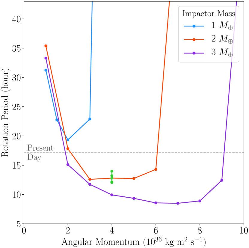
Figure 5: Median rotation periods for particles in the final planets produced by runs with different angular momenta and impactor masses, as given in the legend. The rotation period of each particle is calculated from its tangential velocity and distance from the $z$ axis. All planet particles have negligible velocities in the radial and $z$ directions. The green points show the 2 $M_{\oplus}$-impactor simulations with velocities at infinity of 1–9 km s^-1 instead of the default 5 km s^-1. The dashed horizontal line shows the current rotation rate of Uranus of 17.24 hr (Warwick et al., 1986).

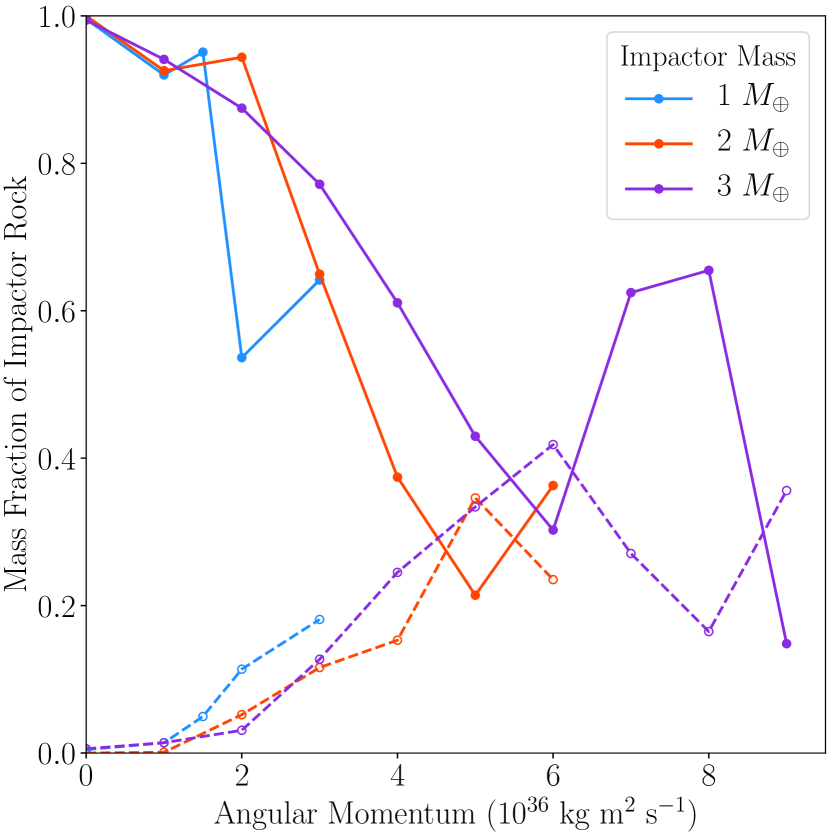
Figure 6: The fraction of impactor rock reaching the core of the final planet ($<1.3$ $R_{\oplus}$, solid lines) or deposited elsewhere in the planet (dashed lines) as a function of impactor mass (as given in the legend) and angular momentum.

The smooth decrease in density seen for both cases in Figure 4 raises the question of how to define the edge of the final planet, which is also slightly flattened due to the rotation that it has acquired. We choose to do this using a friends-of-friends (FoF) algorithm (Davis et al., 1985). This links together particle pairs that are separated by less than some user-defined distance and effectively finds groups of linked particles bounded by an isodensity surface. Using a linking length of 0.3 $R_{\oplus}$ for the low resolution simulations, and scaling by the inverse cube root of the particle number for the high resolution cases leads to a final planet with a radius of $\sim$4 $R_{\oplus}$ and a mass that is insensitive to small changes of the linking length.

A significant amount of material external to this planet is, nevertheless, gravitationally bound to it. We will refer to this as orbiting material. The remaining mass is unbound. The orbiting material can be further divided into that within the Roche radius, which one would expect to accrete relatively quickly onto the planet, and that outside this radius, which is available to form moons. While our simulated planets have Roche radii of 5.5–5.8 $R_{\oplus}$ (for a satellite density of 1 g cm^-3), the Roche radius of present-day Uranus is 6.2 $R_{\oplus}$. When considering the material available for moon formation and the distribution of the post-impact H–He, we will use radii of $6\pm 0.5$ $R_{\oplus}$ to allow for the uncertainty in the planet’s mass and choice of satellite density.

3.2 Resulting Planet

With the final planets defined as described in section 3.1, we can study their rotation rates and internal structures. These properties are discussed in the following two subsections.

3.2.1 Rotation Rate

Figure 5 shows how the rotation period varies with impactor mass and angular momentum. Despite using different proto-Uranus and impactor models from those of S92, we find broadly similar results. There is no 1 $M_{\oplus}$ impactor with a relative velocity at infinity of 5 km s^-1 that can produce a sufficiently rapidly rotating planet. Both 2 and 3 $M_{\oplus}$ impactors are able to satisfy this requirement, provided that the impactor is bringing an angular momentum of at least $2\times 10^{36}$ kg m² s^-1. At first, raising the angular momentum increases the final spin. However, for very high angular momentum values, to the right of the figure, the impactor starts to only graze and eventually misses the target, making it unable to transfer enough of its huge angular momentum.

Our range of simulation numbers of particles shows that these results vary little with numerical resolution, and find them to be already well-determined with the low number of particles adopted by S92. So, the general agreement of (and any differences between) our rotation-rate results and theirs is primarily testing the different models for the colliding bodies and the materials within them, rather than showing numerical effects.

3.2.2 Interior

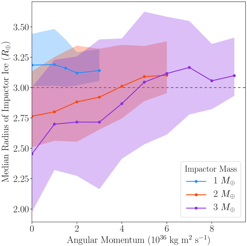
Figure 7: The radius of deposition of the impactor ice as a function of impactor mass and angular momentum. Shaded regions show the 1-$\sigma$ percentile range of the radius distributions. The dashed line shows the approximate radius of the ice-atmosphere boundary in the proto-Uranus targets.

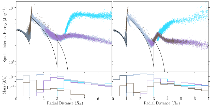
Figure 8: The final radial internal energy profiles for the same relatively head-on (left) and grazing (right) impacts and the same lower-panel histograms of mass per radial bin as in Figure 4.

The density profiles within the planet and their decomposition into material types from the two colliding bodies are shown for the low and high angular momentum impacts in Figure 4. Considering the suite of simulations in full, Figures 6 and 7 show the destinations of the impactor rock and ice within the planet respectively.

It is apparent from Figure 6 that the head-on collisions deliver practically all of their impactor rock to the core. However, as the angular momentum is raised, the fraction of the rock in the impactor that is deposited higher up in the ice layer of the final planet or even into orbit increases significantly. The non-monotonic behaviour at high angular momenta is a consequence of an initially grazing impact sometimes leading to a much more head-on secondary collision of the core after the ice has been stripped and some angular momentum lost. Up to 40% of the rock in 2 and 3 $M_{\oplus}$ impactors can be left embedded in the icy mantle for sufficiently high angular momentum collisions. In our $\sim$$10^{6}$-particle simulations, this rock is present in well-resolved, mostly spherical lumps. Such inhomogeneities will be investigated in detail with higher resolution simulations in the future, but this is beyond the scope of this initial study.

The rock that is added during the collision is generally not distributed isotropically with respect to the centre of the planet. For the 2 $M_{\oplus}$ impactors, 90% of the delivered rock covers only $\sim$50% of the $4\pi$ steradians subtended at the planet’s centre. This increases to $\sim$70% coverage for the 3 $M_{\oplus}$ impactors. The ice that is deposited tends to be more isotropically distributed than the rock, unless the impact is head on in which case 90% of the delivered ice subtends only $\sim$40%$\times 4\pi$ steradians, independent of impactor mass.

Where this impactor ice is deposited may have profound implications for the current internal structure of and heat flow from Uranus. Figure 7 shows the final destinations in radius of the impactor ice. For the 1 $M_{\oplus}$ impactors, the ice is mostly deposited on top of the pre-existing icy mantle, independently of angular momentum, because the impactor is not massive enough to sufficiently disturb the proto-Uranus. However, the larger projectiles are able to inject ice deeper into the final planet, particularly for the lower angular momentum collisions. These more head-on collisions also lead to a slightly thicker zone that is infiltrated by impactor ice (interquartile range spanning $\sim$1 $R_{\oplus}$) than the higher angular momentum cases, which do not penetrate as significantly into the mantle and can spread the impactor ice out into a thinner layer.

In addition to delivering mass, the impactor deposits a significant amount of energy into the final planet. The radial profiles of specific internal energy out to a little beyond the Roche radius are shown in Figure 8, as well as the initial profile with its $\sim$adiabatic ice layer. For both low and high angular momentum collisions, the impactor rock that reaches the edge of the final planet’s core is much hotter than the largely undisturbed proto-Uranus rock. In high angular momentum collisions, a similar temperature inversion is created near the boundary between the ice and atmosphere, where the impactor ice has been delivered, creating a high-entropy layer of hot material. This sub-adiabatic energy gradient is also present in the icy mantle following low angular momentum collisions, but it is less dramatic because of the broader range of radii into which the impactor mass and energy has been deposited.

Investigating the extent and implications of this departure from adiabatic behaviour in the icy mantle compared with that required by evolution models to match the heat flow from present-day Uranus is beyond the scope of this paper. However, our simulations are showing a thermal boundary layer that might suppress convection and provide a blanket to contain the heat in the central region of Uranus (Stevenson, 1986; Podolak & Helled, 2012). This layer of impactor ice could also be a compositional boundary if the icy material is not identical to that in the proto-Uranus. If these results can be usefully fed into evolution models, then this could conceivably lead to another constraint on the types of impact that are able to explain the current Uranus’s thermal state and perhaps also its unusual magnetic field.

3.3 Orbiting Debris Field

If the moons of Uranus are to form from the debris from the collision, then it is necessary to place some rock into orbit beyond the Roche radius. Satellites would also have to form beyond than the co-rotation radius of $\sim$13 $R_{\oplus}$ to not have their orbits decay. Using this instead of the Roche radius for our analysis reduces the amount of material available by a few tens of percent but does not change the overall conclusions. As noted by S92, this task would be made easier by having less differentiated bodies in the first place. Nevertheless, for the higher angular momentum collisions, our simulations succeed in placing significant amounts of rock and ice into the debris field. These clouds of debris are typically quite spherical rather than disk-shaped, with minimum-to-maximum axis ratios between 0.7 and 1, defined using the inertia tensor.

The amounts of rock and ice from the impactor and the proto-Uranus in the debris cloud are shown in Figure 9, as functions of impactor mass and angular momentum. This shows how the more head-on collisions send more proto-Uranus ice into orbit than impactor material. The crossover to impactor ice being more prevalent in orbit occurs at $L\approx 3\times 10^{36}$ kg m² s^-1 for impactors of mass 2 or 3 $M_{\oplus}$. The lowest mass impactor never manages to eject more proto-Uranus ice into orbit than impactor ice.

Grazing impacts sometimes involve multiple significant collisions or near-miss passes, creating large tidal streams of impactor material (Figure 3). For a more massive impactor (and a correspondingly less massive proto-Uranus) the impactor’s core becomes less susceptible to tidal stripping. Consequently, the higher mass impactors become less efficient at placing rock into orbit in this way. It may be that $>$3 $M_{\oplus}$ impactors would be too massive to leave any rock in orbit via this mechanism. These findings are broadly similar to those of S92; though, they were restricted to $<$25 rock particles in orbit and, for their more massive impactor cores, found that only $<$3 $M_{\oplus}$ impactors could be disrupted enough to leave rock in orbit.

3.4 Atmosphere

Most previous studies of atmospheric erosion during impacts have focussed on vertical impacts onto terrestrial planets, where the atmosphere comprises a much smaller mass fraction than is present in our Uranus simulations (Ahrens, 1993). Shuvalov (2009) performed hydrodynamical simulations of oblique collisions of relatively small projectiles (with sizes similar to the atmosphere’s height) into the Earth, finding more atmospheric erosion with more oblique impacts. For sufficiently oblique impacts, the atmospheric loss rose to all the mass above the horizon as seen from the point of impact.

For atmospheric erosion by giant impacts, Genda & Abe (2003) and Schlichting et al. (2015) used a mixture of analytical techniques and one-dimensional numerical simulations to predict that the most important factor is the speed at which the sub-atmospheric surface moves as a result of the shock wave propagating through the planet. This topic has also been little simulated in three dimensions. Liu et al. (2015) tested, to our knowledge, the only previous three-dimensional full-planet models, with two simulations of head-on collisions on super-Earths. The simulations presented here are the first in three dimensions to quantify atmospheric erosion from giant impacts with inter-particle self-gravity as well as the first to test a range of impact angles, leaving much of this topic’s huge parameter space still to be explored.

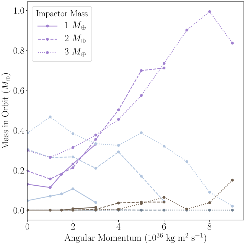
Figure 9: The masses of impactor and proto-Uranus material that are placed into orbit around the final planet (i.e. bound but outside a Roche radius of 6 $R_{\oplus}$) as functions of impactor mass and angular momentum. The line styles refer to the impactor mass and the colours to the material. Light and dark grey show the target’s ice and rock material, respectively, and purple and brown show the same for the impactor.

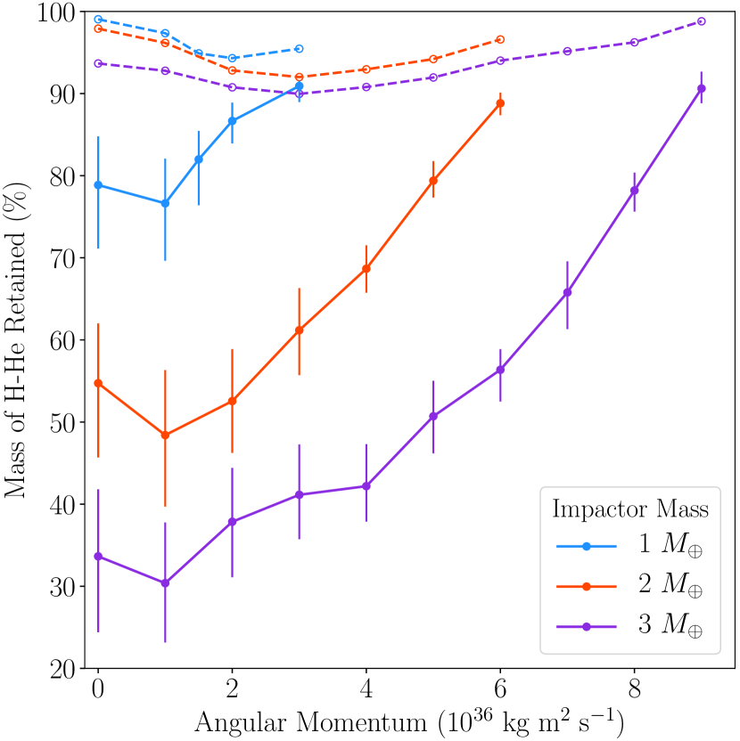
Figure 10: The mass fractions of the H–He atmosphere retained within a Roche radius of 6 $\pm$ 0.5 $R_{\oplus}$ (solid lines) and still bound to the final planet (dashed lines), as functions of impactor mass and angular momentum.

The fractions of the H–He atmosphere that are retained within the Roche radius or bound to the final planet following these giant impacts are shown in Figure 10, as a function of impactor mass and angular momentum. Most of the eroded atmosphere remains bound but can be jettisoned to large radii. There is a monotonic behaviour with larger impactors eroding more atmosphere than smaller ones, but the angular momentum dependence is more complicated. The head-on collisions retain a few more per cent of the atmosphere within the Roche radius than those with $L=1\times 10^{36}$ kg m² s^-1. Up to half of the atmosphere can be sent beyond the Roche radius for 2 $M_{\oplus}$ impactors, and this rises to 70% for $M_{\rm{i}}=3$ $M_{\oplus}$.

The proportion of the proto-Uranus H–He atmosphere that remains bound to the final planet is always at least $\sim$90%, with this minimum value being reached for intermediate values of angular momentum at $\sim$$3\times 10^{36}$ kg m² s^-1. More-grazing impacts lead to significantly higher atmospheric retention because not all the impactor’s energy may be deposited at once, especially if they undergo tidal stripping and multiple less-violent collisions. As such, higher angular momentum giant impacts are less effective at eroding the atmosphere, in contrast with the trends determined by Shuvalov (2009) for the different regime of much smaller impactors. The atmosphere that is ejected by the giant impacts typically originates from near to the impact site, especially in the high angular momentum cases. For the more head-on collisions, some atmosphere can also be lost on the opposite side of proto-Uranus from where the impact occurs, from the high outward velocities of the icy mantle.

4 Conclusions

We have performed SPH simulations to test the hypothesis that Uranus endured a giant impact toward the end of its formation and to investigate the consequences of such an event. Animations of the simulated impacts are available at icc.dur.ac.uk/giant_impacts. We confirm the findings of S92 that the impactor needs to have a mass of greater than 1 $M_{\oplus}$ in order to impart sufficient angular momentum to account for Uranus’ present rotation.

We also investigate where the impactor’s mass and energy are deposited within the planet. Sub-adiabatic temperature gradients are typically created toward the outer regions of the icy mantle, where most of the impactor ice is deposited. Higher impact parameters can even lead to a temperature inversion near the top of the ice layer. These more-grazing collisions also leave the impactor ice further out, in a thin shell near the edge of the icy mantle, whereas $\sim$head-on impacts can implant significant ice up to 0.5 $R_{\oplus}$ further inward and less-isotropically about the centre. These findings may have important implications for understanding the current heat flow (or rather the lack thereof) from Uranus’ interior to its surface.

With our higher resolution simulations, we see significant inhomogeneities in the deposited impactor material, and can also properly resolve the composition of the debris field. The impactor’s ice can be quite isotropically distributed, unlike its rocky core. While most of this rock tends to end up at the top of the core of the final planet, some small chunks become embedded within its icy mantle. For higher angular momentum impacts, significant amounts of rock and ice can be placed into orbit during tidal disruption of the impactor. The efficiency of this process is lower for 3 than 2 $M_{\oplus}$ impactors, since the larger impactors are more able to resist tidal stripping, but could still conceivably provide sufficient material to form Uranus’ current satellites if the angular momentum of the collision exceeds $2\times 10^{36}$ kg m² s^-1.

While less than $\sim$10% of the H–He atmosphere of the proto-Uranus becomes unbound during the collisions, over half can be ejected to beyond the Roche radius. This atmospheric erosion occurs more in lower angular momentum collisions, where the impactor’s energy is deposited all at once and some atmosphere is also lost from the antipode to the impact point.

Higher numerical resolution simulations have allowed us to study a variety of facets of the giant impact hypothesis for producing Uranus’ obliquity in detail, including the first three-dimensional tests of atmospheric loss with inter-particle self-gravity and from off-axis giant impacts. Further work is under way to vary uncertain aspects such as the material EoS and to increase the numerical resolution further with a view to producing an improved prediction for the internal structure and inhomogeneities in the final planet, as well as testing the atmospheric erosion models of Genda & Abe (2003) and Schlichting et al. (2015). The full particle data from the simulations are available on reasonable requests for related studies or collaboration.

Appendix A Equations of State

Hubbard & MacFarlane (1980) (HM80)’s equations of state are expressed in terms of the temperature, $T$, and density, $\rho$. However, the simulation code uses the specific internal energy, $u$, so we must convert between the two. Including the energy contribution from the density:

$$u_{0}(\rho) =\int_{\rho_{0}}^{\rho}\dfrac{P_{0}(\rho)}{\rho^{2}}\,d\rho\;,$$ (A1)

$$u(\rho,T) =u_{0}(\rho)+C_{V}T\;,$$ (A2)

where $u_{0}(\rho)$ and $P_{0}(\rho)$ are the specific internal energy and pressure at zero temperature, $\rho_{0}$ is the material’s zero-pressure density, and $C_{V}$ is the specific heat capacity.

Using HM80’s equations of state and expressions for $C_{V}$ and $P_{0}$, the total pressure can then be tabulated as a function of log($\rho$) and log($u$) for interpolation in the SPH code.

HM80 did not provide expressions for the sound speed, $c_{\rm s}$, so for simplicity we treat the H–He as an ideal gas ($c_{\rm s}=\sqrt{\gamma P/\rho\,}$) and use approximate bulk moduli for the other materials: $c_{\rm s}=\sqrt{2\times 10^{10}~{}\rm{dyn~{}cm}^{-2}/\rho\,}$ for the ice mix, and $c_{\rm s}=\sqrt{2\times 10^{11}~{}\rm{dyn~{}cm}^{-2}/\rho\,}$ for the rocky core, with the density in g cm^-3 (Matsui, 1996).

Appendix B Impact Initial Conditions

Figure 11 shows the relevant input parameters for an impact simulation in the target planet’s rest frame. The chosen parameters for each simulation are the impactor mass, $M_{\rm{i}}$ (and hence target mass, ${M_{\rm{t}}=14.536~{}M_{\oplus}-M_{\rm{i}}}$), total angular momentum, $L$, and a velocity at infinity, $v_{\infty}=5$ km s^-1. From these inputs, we calculate the initial positions and velocities of the two bodies.

Figure 11: The relevant parameters for setting up an impact simulation: the $x$ and $y$ positions of the impactor, its initial velocity, $v_{x}$, and the masses of the proto-Uranus target (t) and impactor (i).

In the centre-of-mass and zero-momentum frame, the total angular momentum is

$$L=L_{z} =M_{\rm{i}}\,v_{x,{\rm{i}}}\,y_{\rm{i}}+M_{\rm{t}}\,v_{x,\rm{t}}\,y_{\rm{t}}$$

$$=v_{x}\,y\left(M_{\rm{i}}\left(1-m^{\prime}\right)^{2}+M_{\rm{t}}\,m^{\prime 2}\right)\;,$$ (B1)

where $m^{\prime}\equiv M_{\rm{i}}/(M_{\rm{i}}+M_{\rm{t}})$.

In order to allow the bodies to be distorted tidally before the impact, we set the initial separation $d$ of the two bodies such that, at the point on the surface of the impactor that is closest to the target, the gravitational force from the target planet is 10 times smaller than that from the impactor:

$$d=\sqrt{\dfrac{10\,M_{\rm{t}}R_{\rm{i}}^{2}}{M_{\rm{i}}}}\;.$$ (B2)

From conservation of energy, the velocity at a distance $d$ is

$$v_{x}=\sqrt{v_{\infty}^{2}+\dfrac{2GM_{\rm{t}}}{d}}\;.$$ (B3)

Finally, $y$ is set using the chosen angular momentum with Equation B1, and $x=\sqrt{d^{2}-y^{2}}$.

References

- Ahrens (1993) Ahrens, T. J. 1993, Annual Review of Earth and Planetary Sciences, 21, 525, doi: 10.1146/annurev.ea.21.050193.002521
- Asphaug et al. (2006) Asphaug, E., Agnor, C. B., & Williams, Q. 2006, Nature, 439, 155, doi: 10.1038/nature04311
- Batalha (2014) Batalha, N. M. 2014, Proceedings of the National Academy of Science, 111, 12647, doi: 10.1073/pnas.1304196111
- Benz et al. (1986) Benz, W., Slattery, W. L., & Cameron, A. G. W. 1986, Icarus, 66, 515, doi: 10.1016/0019-1035(86)90088-6
- Bethkenhagen et al. (2013) Bethkenhagen, M., French, M., & Redmer, R. 2013, J. Chem. Phys., 138, 234504, doi: 10.1063/1.4810883
- Bethkenhagen et al. (2017) Bethkenhagen, M., Meyer, E. R., Hamel, S., et al. 2017, ApJ, 848, 67, doi: 10.3847/1538-4357/aa8b14
- Canup & Ward (2006) Canup, R. M., & Ward, W. R. 2006, Nature, 441, 834, doi: 10.1038/nature04860
- Davis et al. (1985) Davis, M., Efstathiou, G., Frenk, C. S., & White, S. D. M. 1985, ApJ, 292, 371, doi: 10.1086/163168
- Deng et al. (2017) Deng, H., Reinhardt, C., Benitez, F., Mayer, L., & Stadel, J. 2017, ArXiv e-prints. https://arxiv.org/abs/1711.04589
- Fortney et al. (2013) Fortney, J. J., Mordasini, C., Nettelmann, N., et al. 2013, ApJ, 775, 80, doi: 10.1088/0004-637X/775/1/80
- Fressin et al. (2013) Fressin, F., Torres, G., Charbonneau, D., et al. 2013, ApJ, 766, 81, doi: 10.1088/0004-637X/766/2/81
- Fryer et al. (2006) Fryer, C. L., Rockefeller, G., & Warren, M. S. 2006, ApJ, 643, 292, doi: 10.1086/501493
- Genda & Abe (2003) Genda, H., & Abe, Y. 2003, Icarus, 164, 149, doi: 10.1016/S0019-1035(03)00101-5
- Gingold & Monaghan (1977) Gingold, R. A., & Monaghan, J. J. 1977, MNRAS, 181, 375, doi: 10.1093/mnras/181.3.375
- Herant (1994) Herant, M. 1994, Mem. Soc. Astron. Italiana, 65, 1013
- Hosono et al. (2016) Hosono, N., Saitoh, T. R., & Makino, J. 2016, ApJS, 224, 32, doi: 10.3847/0067-0049/224/2/32