D²: Decentralized Training over Decentralized Data

Abstract

While training a machine learning model using multiple workers, each of which collects data from their own data sources, it would be most useful when the data collected from different workers can be unique and different. Ironically, recent analysis of decentralized parallel stochastic gradient descent (D-PSGD) relies on the assumption that the data hosted on different workers are not too different. In this paper, we ask the question: Can we design a decentralized parallel stochastic gradient descent algorithm that is less sensitive to the data variance across workers?

In this paper, we present D², a novel decentralized parallel stochastic gradient descent algorithm designed for large data variance among workers (imprecisely, “decentralized” data). The core of D² is a variance reduction extension of the standard D-PSGD algorithm, which improves the convergence rate from $O\left({\sigma\over\sqrt{nT}}+{(n\zeta^{2})^{\frac{1}{3}}\over T^{2/3}}\right)$ to $O\left({\sigma\over\sqrt{nT}}\right)$ where $\zeta^{2}$ denotes the variance among data on different workers. As a result, D² is robust to data variance among workers. We empirically evaluated D² on image classification tasks where each worker has access to only the data of a limited set of labels, and find that D² significantly outperforms D-PSGD.

1 Introduction

Training machine learning models in a decentralized way has attracted intensive interests recently Lian et al. (2017a); Yuan et al. (2016); Colin et al. (2016). In the decentralized setting, there is a set of workers, each of which collects data from different data sources. Instead of sending all of their data to a centralized place, these workers only communicate with their neighbors. The goal is to get a model that is the same as if all data are collected in a centralized place. Decentralized learning algorithm is important in scenarios in which centralized communication is expensive or not possible, or the underlying communication network has high latency.

For decentralized learning to provide benefit, each user should provides data that is somehow unique, i.e., the variance of data collected from different workers are large. However, many recent theoretical results Lian et al. (2017a, b); Nedic and Ozdaglar (2009); Yuan et al. (2016) all assume a bounded data variance across workers — when data hosted on different workers are very different, these approach could converge slowly, both empirically and theoretically. In this paper, we aim at bringing this discrepancy between the current theoretical understanding and the requirements from some practical scenarios.

In this paper, we present D², a novel decentralized learning algorithm designed to be robust under high data variance. The structure and technique of D² is built upon standard decentralized parallel stochastic gradient descent (D-PSGD), but benefits from an additional variance reduction component. In the D² algorithm, each worker stores the stochastic gradient and its local model in last iterate and linearly combines them with the current stochastic gradient and local model. It results in an improved convergence rate over D-PSGD by eliminating the data variation among workers. In particular, the convergence rate is improved from $O\left({\sigma\over\sqrt{nT}}+{(n\zeta^{2})^{\frac{1}{3}}\over T^{2/3}}\right)$ to $O\left({\sigma\over\sqrt{nT}}\right)$ where $\zeta^{2}$ is the data variation among all workers, $\sigma^{2}$ is the data variance within each worker, $n$ is the number of workers, and $T$ is the number of iterations. We empirically show $D^{2}$ can significantly outperform D-PSGD by training an image classification model where each worker has access to only the data of a limited set of labels.

Throughout this paper, we consider the following decentralized optimization:

$$\min_{\bm{x}\in\mathbb{R}^{N}}\quad f(\bm{x}){\color[rgb]{0,0,0}:=}{1\over n}\sum_{i=1}^{n}\overbrace{\mathbb{E}_{\xi\sim\mathcal{D}_{i}}F_{i}(\bm{x};\xi)}^{=:f_{i}(\bm{x})},$$ (1)

where $n$ is the number of workers and $\mathcal{D}_{i}$ is the local data distribution for worker $i$. All workers are connected to form a connected graph. Each worker can only exchange information with its neighbors.

Definitions and notations

Throughout this paper, we use following notations and definitions:

• $\|\cdot\|_{F}$ denotes the Frobenius norm of matrices.

• $\|\cdot\|$ denotes the $\ell_{2}$ norm for vectors and the spectral norm for matrices.

• $\nabla f(\cdot)$ denotes the gradient of a function $f$.

• $f^{*}$ denotes the optimal solution of (1).

• $\lambda_{i}(\cdot)$ denotes the $i$th largest eigenvalue of a matrix.

• $\bm{x}^{(i)}$ denotes the local model of worker $i$.

• $\nabla F_{i}(\bm{x}^{(i)};\xi^{(i)})$ denotes a local stochastic gradient of worker $i$.

• $\bm{1}=[1,1,\cdots,1]^{\top}\in\mathbb{R}^{n}$ denotes the all-one vector.

• In order to organize the algorithm more clearly, here we define the concatenation of all local variables, stochastic gradients, and their average respectively:

  $$X:= [\bm{x}^{(1)},\dots,\bm{x}^{(n)}]\in\mathbb{R}^{N\times n},$$

  $$\overline{X}:= X\frac{\bm{1}}{n}=\frac{1}{n}\sum_{i=1}^{n}\bm{x}^{(i)},$$

  $$G(X;\xi):= [\nabla F_{1}(\bm{x}^{(1)};\xi^{(1)}),\dots,\nabla F_{n}(\bm{x}^{(n)};\xi^{(n)})]\in\mathbb{R}^{N\times n},$$

  $$\overline{G}(X,\xi):= G(X,\xi)\frac{\bm{1}}{n}=\frac{1}{n}\sum_{i=1}^{n}\nabla F_{i}(\bm{x}^{(i)};\xi^{(i)}),$$

  $$\nabla f(\overline{X}):= \sum_{i=1}^{n}\frac{1}{n}\nabla f_{i}\left({\color[rgb]{0,0,0}\overline{X}}\right),$$

  $$\overline{\nabla f}(X):= \frac{1}{n}\sum_{i=1}^{n}\nabla f_{i}(x^{(i)}),$$

  where $\xi$ is the collection of randomly sampled data from all workers

Organization

This paper is organized as follows: Section 2 reviews related work about the proposed approach; Section 3 introduces the state-of-the-art decentralized stochastic gradient descent method and its convergence rate; Section 4 introduces the proposed algorithm and its intuition why it can improves the state-of-the-art approach; and Section 5; Section 6 validates the proposed approaches via empirical study; and Section 7 concludes this paper.

2 Related work

In this section, we review the stochastic gradient descent algorithm and its decentralized variants, decentralized algorithms, and previous variance reduction technologies in this section.

Stochastic gradient descent (SGD)

The SGD approahces (Ghadimi and Lan, 2013; Moulines and Bach, 2011; Nemirovski et al., 2009) is quite powerful for solving large-scale machine learning problems. It achieves a convergence rate of $O\left({1}/\sqrt{T}\right)$. As an implementation of SGD, the Centralized Parallel Stochastic Gradient Descent (C-PSGD), has been widely used in parallel computation. In C-PSGD, a central worker, whose job is to perform the variable updates, is connected to many leaf workers that are used to compute stochastic gradients in parallel. C-PSGD has been applied to many deep learning frameworks, such as such as CNTK (Seide and Agarwal, 2016), MXNet (Chen et al., 2015), and TensorFlow (Abadi et al., 2016). The convergence rate of C-PSGD is $O\left(\frac{1}{\sqrt{nT}}\right)$, which shows it can achieve linear speedup with regards to the number of leaf workers.

Decentralized algorithms

Centralized algorithms requires a central server to communicate with all other workers (Suresh et al., 2017). In contrast, decentralized algorithms can work on any connected network and only rely on the information exchange between neighbor workers (Kashyap et al., 2007; Lavaei and Murray, 2012; Nedic et al., 2009).

Decentralized algorithms are especially useful under a network with limited bandwidth or high latency. It is more favorable when data privacy is sensitive. These advantages have led to successful applications. The decentralized approach for multi-task reinforcement learning was studied in Omidshafiei et al. (2017); Mhamdi et al. (2017). In Colin et al. (2016), a dual based decentralized algorithm was proposed to solve the pairwise function optimization. Shi et al. (2014) and Mokhtari and Ribeiro (2015) analyzed the decentralized version of the ADMM optimization algorithm. An information theoretic approach was used to analyze decentralization in Dobbe et al. (2017). The decentralized version of (sub-)gradient descent was studied in Nedic and Ozdaglar (2009); Yuan et al. (2016). Its $O(1/\sqrt{T})$ convergence requires a diminishing stepsize or a constant stepsize that depends on the total number of iterations. This phenomenon happens because of the variance between the data in different workers, which we call “outer variance” to differentiate it from the variance in SGD. Recently, there are several deterministic decentralized optimization algorithms that allows a constant stepsize. For example, EXTRA Shi et al. (2015a) is the first modification of decentralized gradient descent that converges under a constant stepsize. Later this algorithm is extended for problems with the sum of smooth and nonsmooth functions at each node Shi et al. (2015b). However, the stepsize depends on both the Lipschitz constant of the differentiable function and the network structure. NIDS is the first algorithm that has a constant network independent stepsize Li et al. (2017). This algorithm was simultaneously proposed by Yuan et al. (2017) for the smooth case only using a different approach. For directed networks, the algorithm DIGing is proposed in Nedić et al. (2017), where two exchanges are needed in each iteration.

Decentralized parallel stochastic gradient descent (D-PSGD)

The D-PSGD algorithm (Nedic and Ozdaglar, 2009; Ram et al., 2010a, b) requires each worker to compute a stochastic gradient and exchange its local model with neighbors. In Duchi et al. (2012), a dual averaging based method is proposed for solving the constrained decentralized SGD optimization. In Yuan et al. (2016), the convergence rate for D-PSGD was analyzed when the gradient is assumed to be bounded. In Lan et al. (2017), a decentralized primal-dual type method was proposed with a computational complexity of $O\left({n}/{\epsilon^{2}}\right)$ for general convex objectives. Lian et al. (2017a) proved that D-PSGD can admits linear speedup w.r.t. number of workers with a similar convergence rate like C-PSGD.

Variance reduction technology

There have been many methods developed for reducing the variance in SGD, including SVRG (Johnson and Zhang, 2013), SAGA (Defazio et al., 2014), SAG (Schmidt et al., 2017), MISO (Mairal, 2015), and mS2GD (Konečnỳ et al., 2016). However, most of these technologies are just designed for the centralized approaches. The DSA algorithm (Mokhtari and Ribeiro, 2016) applies the variance reduction similar to SAGA on strongly convex decentralized optimization problems and proved a linear convergence rate. However, the speedup property is unclear and a table of all stochastic gradients need to be stoblack.

3 Preliminary: decentralized stochastic gradient descent

The decentralized stochastic gradient descent (Lian et al., 2017a; Zhang et al., 2017; Shahrampour and Jadbabaie, 2017) allows each worker (say worker $i$) maintaining its own local variable $\bm{x}^{(i)}$. During each iteration (say, iteration $t$), each worker performs the following steps:

1. Query its neighbors’ local variables.

2. Take weighted average with its local variable and neighbors’ local variables:

   $$\bm{x}^{(i)}_{t+{1\over 2}}=\sum_{j=1}^{n}W_{{\color[rgb]{0,0,0}ij}}\bm{x}^{(j)}_{t}$$

   where $W_{ij}$ is the $(i,j)$ element of the matrix $W$, $W_{ij}=0$ means worker $i$ and worker $j$ are not connected.

3. Perform one stochastic gradient descent step

   $$\bm{x}^{(i)}_{t+1}=\bm{x}^{(i)}_{t+{1\over 2}}-\gamma\nabla F(\bm{x}^{(i)}_{t};\xi^{(i)}_{t})$$

   where $\xi^{(i)}_{t}$ represents the data sampled in worker $i$ at the iteration $t$ following the distribution $\mathcal{D}_{i}$.

From a global point of view, the update rule D-PSGD algorithm can be viewed as

$$X_{t+1}=X_{t}W-\gamma G(X_{t};\xi_{t}).$$

It admits the following rate shown in Theorem 1.

Theorem 1 (Convergence rate of D-PSGD (Lian et al., 2017a)).

Under certain assumptions, the output of D-PSGD admits the following inequality

$$\frac{1-\gamma L}{2T}\sum_{t=0}^{T-1}\mathbb{E}\left\|\overline{\nabla f}(X_{t})\right\|^{2}+\frac{D_{1}}{T}\sum_{t=0}^{T-1}\mathbb{E}\left\|\nabla f\left(\overline{X}_{t}\right)\right\|^{2}\leq\frac{f(0)-f^{\ast}}{\gamma T}+\frac{\gamma L}{2n}\sigma^{2}+\frac{\gamma^{2}L^{2}n\sigma^{2}}{(1-\lambda)D_{2}}+\frac{9\gamma^{2}L^{2}n\varsigma^{2}}{(1-\sqrt{\lambda})^{2}D_{2}},$$

where $\rho$ reflects the property of the network, $D_{1}$ and $D_{2}$ are defined to be

$$D_{1}:= \left(\frac{1}{2}-\frac{9\gamma^{2}L^{2}n}{(1-\sqrt{\rho})^{2}D_{2}}\right)$$

$$D_{2}:= \left(1-\frac{18\gamma^{2}}{(1-\sqrt{\rho})^{2}}nL^{2}\right)$$

and $\sigma$ and $\varsigma$ measure the variation within each worker and among all workers respectively

$$\mathbb{E}_{\xi\sim\mathcal{D}_{i}}\left\|\nabla F_{i}(\bm{x};\xi)-\nabla f_{i}(\bm{x})\right\|^{2}\leqslant \sigma^{2},\quad\forall i,\forall\bm{x},$$ (2)

$${1\over n}\sum_{i=1}^{n}\left\|\nabla f_{i}(\bm{x})-\nabla f(\bm{x})\right\|^{2}\leqslant \zeta^{2},\quad\forall i,\forall\bm{x}.$$ (3)

Choosing the optimal steplength $\gamma=\frac{1}{L+\sigma\sqrt{\frac{K}{n}}+{\color[rgb]{0,0,0}n^{\frac{1}{3}}}\zeta^{\frac{2}{3}}T^{\frac{1}{3}}}$ we have the following convergence rate:

$${1\over T}\sum_{t=1}^{T}\mathbb{E}(\|\nabla f(\overline{X}_{t})\|^{2})\leq{\color[rgb]{0,0,0}O}\left({\sigma\over\sqrt{nT}}+\frac{{\color[rgb]{0,0,0}n^{\frac{1}{3}}}\zeta^{\frac{2}{3}}}{T^{\frac{2}{3}}}{\color[rgb]{0,0,0}+\frac{1}{T}}\right).$$

The proposed D² algorithm can improve the convergence rate by removing the dependence to the global bound of outer variance $\zeta$.

4 The $D^{2}$ algorithm

Algorithm 1 D² algorithm

1:  Input: Initial point $\bm{x}^{(i)}_{0}=\bm{0}$, iteration step length $\gamma$, confusion matrix $W$, and the total number of iterations $T$

2:  for t = 0,1,2,…,T do

3:     Randomly sample $\xi^{(i)}_{t}$ from the local data of the $i$th worker.

4:     Compute a local stochastic gradient based on $\xi^{(i)}_{k}$ and current optimization variable $\bm{x}^{(i)}_{t}:\nabla F_{i}(\bm{x}^{(i)}_{t};\xi^{(i)}_{t})$.

5:     

6:     if t=0 then

7:        $\bm{x}_{t+\frac{1}{2}}^{(i)}=\bm{x}_{t}^{(i)}-\gamma\nabla F_{i}(\bm{x}^{(i)}_{t};\xi^{(i)}_{t}),$

8:     else

9:        $\bm{x}_{t+\frac{1}{2}}^{(i)}=2\bm{x}_{t}^{(i)}-\bm{x}_{t-1}^{(i)}-\gamma\nabla F_{i}(\bm{x}^{(i)}_{t};\xi^{(i)}_{t})+\gamma\nabla F_{i}(\bm{x}^{(i)}_{t-1};\xi^{(i)}_{t-1}).$

10:     end if

11:     Each worker sends $\bm{x}_{t+\frac{1}{2}}^{(i)}$ to its neighbors, and take the weighted average

$$\bm{x}_{t+1}^{(i)}=\sum_{j=1}^{n}W_{{\color[rgb]{0,0,0}ij}}\bm{x}^{(j)}_{t+\frac{1}{2}},$$

where $\bm{x}_{t+\frac{1}{2}}^{(j)}$ is from the worker $j$.

12:  end for

13:  Output: $\frac{1}{n}\sum_{i=1}^{n}\bm{x}^{(i)}_{T}$

In D² algorithm, each worker repeats the following updating rule (say, at iteration $t$) for worker $i$

1. Compute a local stochastic gradient $\nabla F(\bm{x}_{t}^{(i)};\xi_{t}^{(i)})$ by sampling $\xi_{t}^{(i)}$ from distribution $\mathcal{D}^{(i)}$;

2. Update the local model $\bm{x}_{t+\frac{1}{2}}^{(i)}\leftarrow 2\bm{x}_{t}^{(i)}-\bm{x}_{t-1}^{(i)}-\gamma\nabla F_{i}\left(\bm{x}^{(i)}_{t};\xi^{(i)}_{t}\right)+\gamma\nabla F_{i}\left(\bm{x}^{(i)}_{t-1};\xi^{(i)}_{t-1}\right)$ using the local models and stochastic gradients in both the $t$th iteration and the $(t-1)$th iteration.

3. When the synchronization barrier is met, exchange $\bm{x}_{t+\frac{1}{2}}^{(i)}$ with neighbors:

   $$\bm{x}_{t+1}^{(i)}=\sum_{j=1}^{n}W_{{\color[rgb]{0,0,0}ij}}\bm{x}^{(j)}_{t+\frac{1}{2}}.$$

From a global point of view, the update rule of D² can be viewed as:

$$X_{t+1}= \left(2X_{t}-X_{t-1}-\gamma G(X_{t};\xi_{t})+\gamma G(X_{t-1};\xi_{t-1})\right)W.$$

The complete algorithm is summarized in Algorithm 1.

D² essentially runs the stochastic gradient descent step.

To understand the intuition of D², let us consider the mean value $\overline{X}_{t}$, which gets updated just like the standard stochastic gradient descent:

$$\overline{X}_{t+1}= \left(2X_{t}-X_{t-1}-\gamma G(X_{t};\xi_{t})+\gamma G(X_{t-1};\xi_{t-1})\right)W\frac{\bm{1}_{n}}{n},$$

$$\overline{X}_{t+1}= 2\overline{X}_{t}-\overline{X}_{t-1}-\gamma\overline{G}(X_{t};\xi_{t})+\gamma\overline{G}(X_{t-1};\xi_{t-1}),$$

or equivalently

$$\overline{X}_{t+1}-\overline{X}_{t}= \overline{X}_{t}-\overline{X}_{t-1}-\gamma\overline{G}(X_{t};\xi_{t})+\gamma\overline{G}(X_{t-1};\xi_{t-1}),$$

$$= \overline{X}_{1}-\overline{X}_{0}-\gamma\sum_{k=1}^{t}\left(\overline{G}(X_{t};\xi_{t})-\overline{G}(X_{t-1};\xi_{t-1})\right)$$

$$= -\gamma\overline{G}(X_{t};\xi_{t}).\quad\text{(due to $X_{1}=X_{0}-\gamma G(X_{0};\xi_{0})$)}.$$ (4)

Why D² improves the D-PSGD?

Acute reviewers may notice that the D-PSGD algorithm also essentially updates in the form of stochastic gradient descent in (4). Then why D² can improve D-PSGD?

Assume that $X_{t}$ has achieved the optimum $X^{*}:=x^{*}{\bf 1}^{\top}$ with all local models equal to the optimum $x^{*}$ to (1). Then for D-PSGD, the next update will be

$$X_{t+1}=X^{*}-\gamma G(X^{*};\xi_{t}).$$

It shows that the convergence when we approach a solution is affected by $\mathbb{E}[\|G(X^{*};\xi_{t}\|_{F}^{2}]$, which is bounded by

$$\mathcal{O}(\sigma^{2}+\zeta^{2}).$$

as we can see from the following:

$$\mathbb{E}[\|G(X^{*};\xi_{t}\|^{2}_{F}]$$

$$= \mathbb{E}\sum_{i=1}^{n}\left\|\left(\nabla F_{i}(\bm{x}^{*};\xi^{(i)}_{t+1})-\nabla f_{i}(\bm{x}^{*})\right)+\nabla f_{i}(\bm{x}^{*})\right\|^{2}$$

$$\leq 2\mathbb{E}\sum_{i=1}^{n}\left\|\left(\nabla F_{i}(\bm{x}^{*};\xi^{(i)}_{t+1})-\nabla f_{i}(\bm{x}^{*})\right)\right\|^{2}+2\left\|\nabla f_{i}(\bm{x}^{*})-\nabla f(\bm{x}^{*})\right\|^{2}$$

$$\leq 2\sigma^{2}+2\zeta^{2}.$$

Next we apply a similar analysis for D² by assuming that both $X_{t-1}$ and $X_{t}$ have reached the optimal solution $X^{*}$. The next update for $D^{2}$ will be:

$$X_{t+1}=\left(X^{*}-\gamma G(X^{*};\xi_{t})-\gamma G(X^{*};\xi_{t-1})\right)W.$$

It shows that for $D^{2}$, the convergence when we approach a solution relies on the magnitude of $\mathbb{E}[\|G(X^{*};\xi_{t})-G(X^{*};\xi_{t-1}\|^{2}_{F}]$, which is bounded by:

$$\mathcal{O}(\sigma^{2}),$$

which can be seem from:

$$\mathbb{E}[\|G(X^{*};\xi_{t})-G(X^{*};\xi_{t-1})\|^{2}_{F}= \mathbb{E}\sum_{i=1}^{n}\left\|\nabla F_{i}(\bm{x}^{*};\xi_{t}^{(i)})-\nabla f_{i}(\bm{x}^{*})\right\|^{2}-\mathbb{E}\sum_{i=1}^{n}\left\|\nabla F_{i}(\bm{x}^{*};\xi_{t-1}^{(i)})-\nabla f_{i}(\bm{x}^{*})\right\|^{2}$$

$$\leq 2\sigma^{2}.$$

5 Theoretical guarantee

This section provides the theoretical guarantee for the proposed D² algorithm. We first give the assumptions requiblack below.

Assumption 1.

Throughout this paper, we make the following commonly used assumptions:

1. Lipschitzian gradient: All function $f_{i}(\cdot)$’s are with $L$-Lipschitzian gradients.

2. Bounded variance: Assume bounded variance of stochastic gradient within each worker

   $$\mathbb{E}_{\xi\sim\mathcal{D}_{i}}\left\|\nabla F_{i}(\bm{x};\xi)-\nabla f_{i}(\bm{x})\right\|^{2}\leqslant \sigma^{2},\quad\forall i,\forall\bm{x}.$$

3. Symmetric confusion matrix: The confusion matrix $W$ is symmetric and satisfies $W\bm{1}=\bm{1}$.

4. Spectral gap: Let the eigenvalues of $W\in\mathbb{R}^{n\times n}$ be $\lambda_{1}\geq\lambda_{2}\geq\cdots\geq\lambda_{n}$. Denote by for short

   $$\lambda:=\max\limits_{i\in\{2,\cdots,n\}}\lambda_{i}=\lambda_{2}.$$

   We assume $\lambda<1$ and $\lambda_{n}>-\frac{1}{3}$.

5. Initialization: W.l.o.g., assume all local variables are initialized by zero, that is, $X_{0}=0$.

Existing decentralized consensus algorithms (Shi et al., 2015b; Li et al., 2017) use a modification of the doubly stochastic matrix such that $\lambda>0$, i.e., choose $W=(\tilde{W}+I)/2$ where $W$ is a doubly stochastic matrix. Recently, Li and Yan (2017) show that $\lambda_{n}>-1/3$ is optimal in the convergence of EXTRA. However, the optimal $\lambda_{n}$ for NIDS (Li et al., 2017) is unknown. In this paper, we proved that $-\frac{1}{3}$ is the infimum of $\lambda_{n}$, and when it blackuces to deterministic case, this condition is weaker than that in Li et al. (2017). This is important, because we actually can use a $W$ that performs better.

Given Assumption 1, we have following convergence guarantee for $D^{2}$:

Theorem 2 (Convergence of Algorithm 1).

Choose the steplength $\gamma$ in Algorithm 1 to be a constant satisfying $1-24C_{2}\gamma^{2}L^{2}>0$. Under Assumption 1, we have the following convergence rate for Algorithm 1:

$$A_{1}\|\nabla f(\bm{0})\|^{2}+\sum_{t=1}^{T-1}\left(\mathbb{E}\|\nabla f({\color[rgb]{0,0,0}\overline{X}_{t}})\|^{2}+A_{2}\mathbb{E}\|\overline{\nabla f}(X_{t})\|^{2}\right)$$

$$\leq \frac{2(f(0)-f^{*})}{\gamma}+\frac{LT\gamma}{n}\sigma^{2}+\frac{6L^{2}C_{1}\gamma^{2}\zeta_{0}^{2}}{C_{3}}+\frac{12L^{2}C_{2}\gamma^{2}\sigma^{2}T}{C_{3}}+\frac{6L^{2}C_{2}\gamma^{4}L^{2}\sigma^{2}T}{nC_{3}}+\frac{6L^{2}C_{1}\gamma^{2}\sigma^{2}}{C_{3}},$$ (5)

where

$$\zeta_{0}:= \frac{1}{n}\sum_{i=1}^{n}\|\nabla f_{i}(\bm{0})-\nabla f(\bm{0})\|^{2},$$

$$v:= \lambda_{n}-\sqrt{\lambda_{n}^{2}-\lambda_{n}},$$

$$C_{1}:= \max\left\{\frac{1}{1-|v|^{2}},\frac{1}{(1-\lambda)^{2}}\right\}\geq 1,$$

$$C_{2}:= \max\left\{\frac{\lambda_{n}^{2}}{(1-|v|^{2})},\frac{\lambda^{2}}{(1-\sqrt{\lambda})^{2}(1-\lambda)}\right\},$$

$$C_{3}:= 1-24C_{2}\gamma^{2}L^{2},$$

$$A_{1}:= 1-\frac{6L^{2}C_{1}\gamma^{2}}{C_{3}},$$

$$A_{2}:= 1-L\gamma-\frac{6L^{2}C_{2}\gamma^{4}L^{2}}{C_{3}}.$$

By appropriately specifying the step length $\gamma$ we reach the following corollary:

Corollary 3.

Choose the step length $\gamma$ in Algorithm 1 to be $\gamma=\frac{1}{8\sqrt{C_{2}}L+6\sqrt{C_{1}}L+\sigma\sqrt{\frac{T}{n}}}$, where $C_{1}$ and $C_{2}$ are defined in Theorem 2. Under Assumption 1, the following convergence rate holds

$$\frac{1}{T}\sum_{t=0}^{T}\mathbb{E}\|\nabla f(\overline{X_{t}})\|^{2}\lesssim \frac{\sigma}{\sqrt{nT}}+\frac{1}{T}+\frac{\zeta_{0}^{2}}{T+\sigma^{2}T^{2}}+\frac{\sigma^{2}}{1+\sigma^{2}T},$$

where $\zeta_{0}$ is defined in Theorem 2 and we treat $f(0)-f^{*}$, $L$, $\lambda_{n}$, and $\lambda$ as constants.

Note that we can obtain even better constants by choosing different parameters and applying tighter inequalities, however, the main result of this corollary is to show the order of the convergence. We highlight a few key observations from our theoretical results in the following.

Tightness of the convergence rate

Setting $\sigma=0$ and $\zeta_{0}=0$, which blackuces the VR-SGD to a normal GD algorithm, we shall see that the convergence rate becomes $O\left(\frac{1}{T}\right)$, which is exactly the rate of GD.

Linear speedup

Since the leading term of the convergence rate is $O\left(\frac{1}{\sqrt{nT}}\right)$, which is consistent with the convergence rate of C-PSGD, this indicates that we would achieve a linear speed up with respect to the number of nodes.

Consistent with NIDS

In NIDS (Li and Yan, 2017), the term depends on $\zeta_{0}$ in the convergence rate is $O\left(\frac{\zeta^{2}_{0}}{T}\right)$. While the corresponding term in $D^{2}$ is $O\left(\frac{\zeta_{0}^{2}}{T+\sigma^{2}T^{2}}\right)$, which indicates when our algorithm is consistent with NIDS because in NIDS $\sigma$ is consideblack to be 0.

Superiority over D-PSGD

When compablack to D-PSGD, the convergence rate of $D^{2}$ only depends on $\zeta_{0}$, and the corresponding decaying rate is $\frac{\zeta_{0}}{T^{2}}$. Whereas in D-PSGD (Lian et al., 2017a), we need to assume an upper bound for the global variance between different nodes’ dataset, and its influence can be compablack to $\sigma^{2}$, the inner variance of each node itself. This means we can always achieve a much better convergence rate than D-PSGD.

6 Experiments

We evaluate the effectiveness of D² by comparing it with both centralized and decentralized SGD algorithms.

6.1 Experiment Settings

We conduct experiments in two settings.

1. TransferLearning: We test the case that each worker has access to a local pre-trained neural network as feature extractor, and we want to train a logistic regression model among all these workers. In our experiment, we select the first 16 classes of ImageNet and use InceptionV4 as the feature extractor to extract 2048 features for each image. We conduct data augmentation and generate a blurblack version for each image. In total this datasaet contains 16$\times$1300$\times$2 images.

2. LeNet: We test the case that all workers collaboratively train a neural network model. We train a LeNet on the CIFAR10 dataset. In total this dataset contains 50,000 images of size 32$\times$32.

One caveat of training more recent neural networks is that modern architectures often have a batch normalization layer, which inherently assumes that the data distribution is uniform across different batches, which is not the case that we are interested in. In principle, we could also flow the batch information through the network in a decentralized way; however, we leave this as future work.

By default, each worker only has exclusive access to a subset of classes. For TransferLearning, we use 16 workers and each worker has access to one class; for LeNet, we use 5 workers and each worker has access to two classes. For comparison, we also consider a case when the datasets is first shuffled and then uniformly partitioned among all the workers, we call this the shuffled case, and the default one the unshuffled case. We use a ring topology for both experiments.

Parameter Tuning. For TransferLearning, we use constant learning rates and tune it from {0.01, 0.025, 0.05, 0.075, 0.1}. For LeNet, we use constant learning rate 0.05 which is tuned from {0.5, 0.1, 0.05, 0.01} for centralized algorithms and batch size 128 on each worker.

Metrics. In this paper, we mainly focus on the convergence rate of different algorithms instead of the wall clock speed. This is because the implementation of D² is a minor change over the standard D-PSGD algorithm, and thus they has almost the same speed to finish one epoch of training, and both are no slower than the centralized algorithm. When the network has high latency, if a decentralized algorithm ($D^{2}$ or D-PSGD) converges with a similar speed as the centralized algorithm, it can be up to one order of magnitude faster Lian et al. (2017a). However, the convergence rate depending on the “outer variance” is different for both algorithms.

6.2 Unshuffled Case

We are mostly interested in the unshuffled case, in which the data variation across workers is maximized. Figure 1 shows the result. In the unshuffled case, we see that the D-PSGD algorithm convergences slower than the centralized case. This is consistent with the original D-PSGD paper (Lian et al., 2017a). On the other hand, D² converges much faster than D-PSGD, and achieves almost the same loss as the centralized algorithm. For the LeNet case, each worker only has access to data of assigned two labels, which means the data variation is very large. The D-PSGD does not converge with the the given learning rate 0.05.

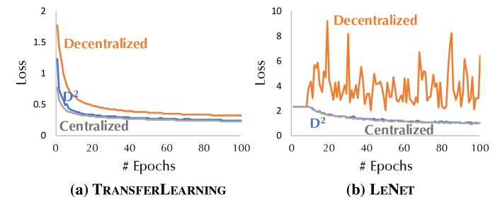
Figure 1: Convergence of Different Distributed Training Algorithms (Unshuffled Case).

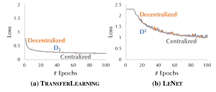
Figure 2: Convergence of Different Distributed Training Algorithms (Shuffled Case).

6.3 Shuffled Case

As a sanity check, Figure 2 shows the result of three different algorithms on the shuffled data. In this case, the data variation of among workers is small (in expectation, they are drawn from the same distribution). We see that, all strategies have similar convergence rate. This validate that the D² algorithm is more effective for larger data variation between different workers.

7 Conclusion

In this paper, we propose a decentralized algorithm, namely, D² algorithm. D² algorithm integrates the D-PSGD algorithm with the variance reduction technology, by which we improves the convergence rate of D-PSGD. The variance reduction technology used in this paper is different from the commonly used ones such as SVRG and SAGA, that are designed for centralized approaches. Experiments validate the advantage of D² over D-PSGD — D² converges with a rate that is similar to centralized SGD while D-PSGD does not converge to the a solution with a similar quality when the data variance is large. While being robust to large data variance among workers, the same performance benefit of D-PSGD over the centralized strategy still holds for D².

Supplemental Materials

This supplement material includes the proofs for Theorem 2.

Because the confusion matrix $W$ is symmetric, it can be decomposed as $W=P\Lambda P^{\top}$, where $P=\left(\bm{v}_{1},\bm{v}_{2},\cdots,\bm{v}_{n}\right)$ is an orthogonal matrix, i.e., $P^{\top}P=PP^{\top}=I$, and $\Lambda=\textnormal{diag}\{\lambda_{1},\dots,\lambda_{n}\}$ is a diagonal matrix with diagonal entries being the eigenvalues of $W$ in the nonincreasing order. Then applying the decomposition to the iteration (from $W_{t}$ and $W_{t-1}$ to $W_{t+1}$)

$$X_{t+1}=2X_{t}W-X_{t-1}W-\gamma G(X_{t};\xi_{t})W+\gamma G(X_{t-1};\xi_{t-1})W$$

gives

$$X_{t+1}= 2X_{t}P\Lambda P^{\top}-X_{t-1}P\Lambda P^{\top}-\gamma G(X_{t};\xi_{t})P\Lambda P^{\top}+\gamma G(X_{t-1};\xi_{t-1})P\Lambda P^{\top}.$$

Denote $Y_{t}=X_{t}P$, $H(X_{t};\xi_{t})=G(X_{t};\xi_{t})P$, and use $y_{t}^{(i)}$ and $h_{t}^{(i)}$ to indicate the $i$-th column of $Y_{t}$ and $H(X_{t};\xi_{t})$, respectively. Then

$$Y_{t+1}= 2Y_{t}\Lambda-Y_{t-1}\Lambda-\gamma H(X_{t};\xi_{t})\Lambda+\gamma H(X_{t-1};\xi_{t-1})\Lambda,$$ (6)

or in the columns of $Y_{t}$ and $H(X_{t};\xi_{t})$,

$$y_{t+1}^{(i)}= \lambda_{i}(2y_{t}^{(i)}-y_{t-1}^{(i)}-\gamma h_{t}^{(i)}+\gamma h_{t-1}^{(i)}).$$ (7)

From the properties of $W$ in Assumption 1 and the decomposition, we have $\lambda_{1}=1$ and $\bm{v}_{1}=\frac{1}{\sqrt{n}}(1,1,\cdots,1)^{\top}$. Therefore $y_{t}^{(1)}=\overline{X}_{t}\sqrt{n}$. For all other eigenvalues $-\frac{1}{3}<\lambda_{i}<1$, the equation (7) shows that all $y_{t}^{(i)}$ would “decay to zero”, which explains how the confusion matrix works.

Lemma 4.

Given two non-negative sequences $\{a_{t}\}_{t=1}^{\infty}$ and $\{b_{t}\}_{t=1}^{\infty}$ that satisfying

$$a_{t}=\sum_{s=1}^{t}\rho^{t-s}b_{s},$$ (8)

with $\rho\in[0,1)$, we have

$$S_{k}:=\sum_{t=1}^{k}a_{t}\leq \sum_{s=1}^{k}\frac{b_{s}}{1-\rho},$$

$$D_{k}:=\sum_{t=1}^{k}a_{t}^{2}\leq \frac{1}{(1-\rho)^{2}}\sum_{s=1}^{k}b_{s}^{2}.$$

Proof.

$$S_{k}:=\sum_{t=1}^{k}a_{t}= \sum_{t=1}^{k}\sum_{s=1}^{t}\rho^{t-s}b_{s}=\sum_{s=1}^{k}\sum_{t=s}^{k}\rho^{t-s}b_{s}=\sum_{s=1}^{k}\sum_{t=0}^{k-s}\rho^{t}b_{s}\leq\sum_{s=1}^{k}{b_{s}\over 1-\rho}.$$ (9)

$$D_{k}:=\sum_{t=1}^{k}a_{t}^{2}= \sum_{t=1}^{k}\sum_{s=1}^{t}\rho^{t-s}b_{s}\sum_{r=1}^{t}\rho^{t-r}b_{r}=\sum_{t=1}^{k}\sum_{s=1}^{t}\sum_{r=1}^{t}\rho^{2t-s-r}b_{s}b_{r}$$

$$\leq \sum_{t=1}^{k}\sum_{s=1}^{t}\sum_{r=1}^{t}\rho^{2t-s-r}{b_{s}^{2}+b_{r}^{2}\over 2}=\sum_{t=1}^{k}\sum_{s=1}^{t}\sum_{r=1}^{t}\rho^{2t-s-r}b_{s}^{2}$$

$$\leq {1\over 1-\rho}\sum_{t=1}^{k}\sum_{s=1}^{t}\rho^{t-s}b_{s}^{2}\leq{1\over(1-\rho)^{2}}\sum_{s=1}^{k}b_{s}^{2}$$ (10)

where the last inequality holds because of (9). ∎

Lemma 5.

For any matrix $X_{t}\in\mathbb{R}^{N\times n}$, we have

$$\sum_{i=2}^{n}\left\|X_{t}\bm{v}^{(i)}\right\|^{2}\leq \sum_{i=1}^{n}\left\|X_{t}\bm{v}^{(i)}\right\|^{2}=\left\|X_{t}\right\|^{2}_{F}$$

$$\sum_{i=1}^{n}\left\|X_{t}P^{\top}\bm{e}^{(i)}\right\|^{2}= \left\|X_{t}P^{\top}\right\|^{2}_{F}=\left\|X_{t}\right\|^{2}_{F}$$

where $\bm{e}^{(i)}\in\mathbb{R}^{n\times 1}$ with the $i$-th component being 1 and all others being 0.

Proof.

From the definition of the Frobenius norm for a matrix, we have

$$\sum_{i=1}^{n}\left\|X_{t}\bm{v}^{(i)}\right\|^{2}= \|X_{t}P\|_{F}^{2}=Tr\left(X_{t}PP^{\top}X_{t}^{\top}\right)=Tr\left(X_{t}X_{t}^{\top}\right)=\left\|X_{t}\right\|^{2}_{F}.$$

Since $\left\|X_{t}\bm{v}^{(1)}\right\|^{2}\geq 0$, so

$$\sum_{i=2}^{n}\left\|X_{t}\bm{v}^{(i)}\right\|^{2}\leq\sum_{i=1}^{n}\left\|X_{t}\bm{v}^{(i)}\right\|^{2}=\sum_{i=1}^{n}\left\|X_{t}\right\|^{2}_{F}.$$

In the same way, we have

$$\sum_{i=1}^{n}\left\|X_{t}P^{\top}\bm{e}^{(i)}\right\|^{2}=\left\|X_{t}P^{\top}\right\|^{2}_{F}=\left\|X_{t}\right\|^{2}_{F}.$$

The result is proved. ∎

Lemma 6.

Given $\rho\in(-{1\over 3},0)\bigcup(0,1)$, for any two sequence $\{a_{t}\}_{t=0}^{\infty}$ and $\{b_{t}\}_{t=0}^{\infty}$ that satisfy

$$a_{0}= b_{0}=0,$$

$$a_{1}= b_{1},$$

$$a_{t+1}= \rho(2a_{t}-a_{t-1})+b_{t}-b_{t-1},\quad\forall t\geq 1,$$

we have

$$a_{t+1}=a_{1}\left(\frac{u^{t+1}-v^{t+1}}{u-v}\right)+\sum_{s=1}^{t}\beta_{s}\frac{u^{t-s+1}-v^{t-s+1}}{u-v},\quad\forall t\geq 0,$$

where

$$\beta_{s}=b_{s}-b_{s-1},\quad u=\rho+\sqrt{\rho^{2}-\rho},\quad v=\rho-\sqrt{\rho^{2}-\rho}.$$

More specifically, if $0<\rho<1$, we have

$$a_{t+1}\sin{\theta}=a_{1}\rho^{t/2}\sin{[(t+1)\theta]}+\sum_{s=1}^{t}\beta_{s}\rho^{(t-s)/2}\sin{[(t+1-s)\theta]},\quad\forall t\geq 0$$

where

$$\beta_{s}= b_{s}-b_{s-1},\quad\theta=\arccos(\sqrt{\rho}).$$

Proof.

When $t=0$, the results is easy to verify. Next we consider the case $t\geq 1$. Since

$$a_{t+1}=2\rho a_{t}-\rho a_{t-1}+\beta_{t},$$

We can find

$$u=\rho+\sqrt{\rho^{2}-\rho},\quad v=\rho-\sqrt{\rho^{2}-\rho},$$

such that

$$a_{t+1}-ua_{t}= (a_{t}-ua_{t-1})v+\beta_{t}.$$ (11)

Note that $u$ and $v$ are complex numbers when $0<\rho<1$. That is

$$u=\sqrt{\rho}e^{i\theta},\quad v=\sqrt{\rho}e^{-i\theta},$$

with $\theta=\arccos{(\sqrt{\rho})}$.

Recursively applying (11) gives

$$a_{t+1}-ua_{t}= (a_{t}-ua_{t-1})v+\beta_{t}=(a_{t-1}-ua_{t-2})v^{2}+\beta_{t-1}v+\beta_{t}$$

$$= (a_{1}-ua_{0})v^{t}+\sum_{s=1}^{t}\beta_{s}v^{t-s}$$

$$= a_{1}v^{t}+\sum_{s=1}^{t}\beta_{s}v^{t-s}.\quad\text{(due to $a_{0}=0$)}$$

Diving both sides by $u^{t+1}$, we obtain

$$\frac{a_{t+1}}{u^{t+1}}= \frac{a_{t}}{u^{t}}+u^{-(t+1)}\left(a_{1}v^{t}+\sum_{s=1}^{t}\beta_{s}v^{t-s}\right)$$

$$= \frac{a_{t-1}}{u^{t-1}}+u^{-t}\left(a_{1}v^{t-1}+\sum_{s=1}^{t-1}\beta_{s}v^{t-1-s}\right)+u^{-(t+1)}\left(a_{1}v^{t}+\sum_{s=1}^{t}\beta_{s}v^{t-s}\right)$$

$$= \frac{a_{1}}{u}+\sum_{k=1}^{t}u^{-k-1}\left(a_{1}v^{k}+\sum_{s=1}^{k}\beta_{s}v^{k-s}\right)$$

Then we multiply both sides by $u^{t+1}$ and have

$$a_{t+1}= a_{1}u^{t}+\sum_{k=1}^{t}u^{t-k}\left(a_{1}v^{k}+\sum_{s=1}^{k}\beta_{s}v^{k-s}\right)$$

$$= a_{1}u^{t}\left(1+\sum_{k=1}^{t}\left(\frac{v}{u}\right)^{k}\right)+u^{t}\sum_{k=1}^{t}\sum_{s=1}^{k}\beta_{s}v^{-s}\left(\frac{v}{u}\right)^{k}$$

$$= a_{1}u^{t}\sum_{k=0}^{t}\left(\frac{v}{u}\right)^{k}+u^{t}\sum_{s=1}^{t}\sum_{k=s}^{t}\beta_{s}v^{-s}\left(\frac{v}{u}\right)^{k}\quad\text{(due to $\sum_{k=1}^{t}\sum_{s=1}^{k}a_{s}b_{k}=\sum_{s=1}^{t}\sum_{k=s}^{t}a_{s}b_{k}$)}$$

$$= a_{1}u^{t}\left(\frac{1-\left(\frac{v}{u}\right)^{t+1}}{1-\frac{v}{u}}\right)+u^{t}\sum_{s=1}^{t}\beta_{s}v^{-s}\left(\frac{v}{u}\right)^{s}\frac{1-\left(\frac{v}{u}\right)^{t-s+1}}{1-\frac{v}{u}}$$

$$= a_{1}\left(\frac{u^{t+1}-v^{t+1}}{u-v}\right)+\sum_{s=1}^{t}\beta_{s}\frac{u^{t-s+1}-v^{t-s+1}}{u-v}.$$

When $\rho\in(0,1)$, since $u=\sqrt{\rho}e^{i\theta}$ and $v=\sqrt{\rho}e^{-i\theta}$, we have

$$a_{t+1}=a_{1}\rho^{t/2}\frac{\sin{[(t+1)\theta]}}{\sin{\theta}}+\sum_{s=1}^{t}\beta_{s}\rho^{(t-s)/2}\frac{\sin{[(t-s+1)\theta]}}{\sin{\theta}}.$$

The result is proved. ∎

Lemma 7.

Under Assumption 1, we have

$$\left(1-24C_{2}\gamma^{2}L^{2}\right)\sum_{i=1}^{n}\sum_{t=0}^{T}\left\|\overline{X}_{t}-\bm{x}_{t}^{(i)}\right\|^{2}$$

$$\leq 2C_{1}\|X_{1}\|^{2}_{F}+12C_{2}\gamma^{2}n\sigma^{2}T+6C_{2}\gamma^{4}L^{2}\sigma^{2}T+6C_{2}\gamma^{4}L^{2}n\sum_{t=1}^{T-1}\left\|\overline{\nabla f}(X_{t})\right\|^{2},$$

where $\gamma$, $L$, $\sigma$, $\theta$, $C_{1}$ and $C_{2}$ are defined in Theorem 2.

Proof.

To estimate the difference of the local models and the global mean model, we have

$$\sum_{i=1}^{n}\left\|\overline{X}_{t}-\bm{x}_{t}^{(i)}\right\|^{2}= \sum_{i=1}^{n}\left\|X_{t}\bm{e}^{(i)}-X_{t}\frac{\bm{1}_{n}}{n}\right\|^{2}=\|X_{t}-X_{t}{\bm{1}_{n}\bm{1}_{n}^{\top}\over n}\|_{F}^{2}=\|X_{t}PP^{\top}-X_{t}\bm{v}_{1}\bm{v}_{1}^{\top}\|_{F}^{2}$$

$$= \left\|X_{t}P\begin{pmatrix}&0,&0,&0,&\cdots,&0\\ &0,&1,&0,&\cdots,&0\\ &0,&0,&1,&\cdots,&0\\ &{5}\\ &0,&0,&0,&\cdots,&1\end{pmatrix}\right\|^{2}_{F}$$

$$= \sum_{i=2}^{n}\left\|y_{t}^{(i)}\right\|^{2},$$ (12)

where $y_{t}^{(i)}$ is the $i$-th column of $X_{t}P$. Note that we have, from (7),

$$y_{t+1}^{(i)}=\lambda_{i}(2y_{t}^{(i)}-y_{t-1}^{(i)}-\gamma h_{t}^{(i)}+\gamma h_{t-1}^{(i)})=\lambda_{i}(2y_{t}^{(i)}-y_{t-1}^{(i)})+\lambda_{i}\beta_{t}^{(i)},$$

where $\beta_{t}^{(i)}=-\gamma h_{t}^{(i)}+\gamma h_{t-1}^{(i)}$. For all $y^{(i)}$ that corresponding to $-\frac{1}{3}<\lambda_{i}<0$, Lemma 6 shows

$$y_{t+1}^{(i)}= y_{1}^{(i)}\left(\frac{u^{t+1}_{i}-v_{i}^{t+1}}{u_{i}-v_{i}}\right)+\lambda_{i}\sum_{s=1}^{t}\beta_{s}^{(i)}\frac{u_{i}^{t-s+1}-v_{i}^{t-s+1}}{u_{i}-v_{i}},$$

where $u_{i}=\lambda_{i}+\sqrt{\lambda^{2}_{i}-\lambda_{i}}$ and $v_{i}=\lambda_{i}-\sqrt{\lambda^{2}_{i}-\lambda_{i}}$. Therefore, we have

$$\left\|y_{t+1}^{(i)}\right\|^{2}\leq 2\left\|y_{1}^{(i)}\right\|^{2}\left(\frac{u_{i}^{t+1}-v_{i}^{t+1}}{u_{i}-v_{i}}\right)^{2}+2\lambda_{i}^{2}\left(\sum_{s=1}^{t}\left\|\beta_{s}^{(i)}\right\|\left|\frac{u_{i}^{t-s+1}-v_{i}^{t-s+1}}{u_{i}-v_{i}}\right|\right)^{2}.$$ (13)

For $\left|\frac{u_{i}^{n+1}-v_{i}^{n+1}}{u_{i}-v_{i}}\right|$, we have

$$\left|\frac{u_{i}^{n+1}-v_{i}^{n+1}}{u_{i}-v_{i}}\right|\leq|v_{i}|^{n}\left|\frac{u_{i}\left(\frac{u_{i}}{v_{i}}\right)^{n}-v_{i}}{u_{i}-v_{i}}\right|\leq|v_{i}|^{n}\quad\text{(due to $|u_{i}|<|v_{i}|$)}.$$

Using (13), we obtain

$$\left\|y_{t+1}^{(i)}\right\|^{2}\leq 2\left\|y_{1}^{(i)}\right\||v_{i}|^{2t}+2\lambda_{i}^{2}\left(\sum_{s=1}^{t}\left\|\beta_{s}^{(i)}\right\||v_{i}|^{t-s}\right)^{2}.$$

Summing from $t=0$ to $t=T-1$ gives

$$\sum_{t=0}^{T-1}\left\|y_{t+1}^{(i)}\right\|^{2}=\sum_{t=1}^{T}\left\|y_{t}^{(i)}\right\|^{2}\leq 2\left\|y_{1}^{(i)}\right\|\sum_{t=0}^{T-1}|v_{i}|^{2t}+2\lambda_{i}^{2}\sum_{t=1}^{T-1}\left(\sum_{s=1}^{t}\left\|\beta_{s}^{(i)}\right\||v_{i}|^{t-s}\right)^{2}.$$

Denote $a_{t}=\sum_{s=1}^{t}\left\|\beta_{s}^{(i)}\right\||v_{i}|^{t-s}$, which has the same structure as the sequence in Lemma 4. Therefore, when $\lambda_{i}<0$, we have

$$\sum_{t=1}^{T}\left\|y_{t}^{(i)}\right\|^{2}\leq \frac{2\left\|y_{1}^{(i)}\right\|}{1-|v_{i}|^{2}}+\frac{2\lambda_{i}^{2}}{(1-|v_{i}|)^{2}}\sum_{t=1}^{T-1}\left\|\beta_{t}^{(i)}\right\|^{2}$$

$$\leq \frac{2\left\|y_{1}^{(i)}\right\|}{1-|v|^{2}}+\frac{2\lambda_{n}^{2}}{(1-|v|)^{2}}\sum_{t=1}^{T-1}\left\|\beta_{t}^{(i)}\right\|^{2},$$ (14)

where $v=\lambda_{n}-\sqrt{\lambda^{2}_{n}-\lambda_{n}}$.

For all $y^{(i)}$ that satisfies $0\leq\lambda_{i}<1$, from (7) and Lemma 6, we have

$$y_{t+1}^{(i)}\sin{\theta_{i}}=y_{1}^{(i)}\lambda_{i}^{t/2}\sin{[(t+1)\theta_{i}]}+\lambda_{i}\sum_{s=1}^{t}\beta_{s}^{(i)}\lambda_{i}^{(t-s)/2}\sin{[(t+1-s)\theta_{i}]},$$

where $\beta_{s}^{(i)}=-\gamma h_{s}^{(i)}+\gamma h_{s-1}^{(i)}$ and $\theta_{i}=\arccos(\sqrt{\lambda_{i}})$.

Then

$$\left\|y_{t+1}^{(i)}\right\|^{2}\sin^{2}\theta_{i}\leq 2\left\|y_{1}^{(i)}\right\|^{2}\lambda_{i}^{t}\sin^{2}[(t+1)\theta_{i}]+2\lambda_{i}^{2}\left(\sum_{s=1}^{t}\left\|\beta_{s}^{(i)}\sin{[(t+1-s)\theta_{i}]}\right\|\lambda_{i}^{(t-s)/2}\right)^{2}$$

$$\leq 2\left\|y_{1}^{(i)}\right\|^{2}\lambda_{i}^{t}+2\lambda_{i}^{2}\left(\sum_{s=1}^{t}\|\beta_{s}^{(i)}\|\lambda_{i}^{(t-s)/2}\right)^{2},$$

Summing from $t=0$ to $T-1$ gives

$$\sum_{t=0}^{T-1}\left\|y_{t+1}^{(i)}\right\|^{2}\sin^{2}\theta_{i}=\sum_{t=1}^{T}\left\|y_{t}^{(i)}\right\|^{2}\sin^{2}\theta_{i}\leq 2\left\|y_{1}^{(i)}\right\|^{2}\sum_{t=0}^{T-1}\lambda_{i}^{t}+2\lambda_{i}^{2}\sum_{t=1}^{T-1}\left(\sum_{s=1}^{t}\|\beta_{s}^{(i)}\|\lambda_{i}^{(t-s)/2}\right)^{2}$$

From Lemma 4, $\sum_{s=1}^{t}\|\beta_{s}^{(i)}\|\lambda_{i}^{(t-s)/2}$ has the same structure as the sequence in Lemma 4, so we have

$$\sum_{t=1}^{T}\left\|y_{t}^{(i)}\right\|^{2}\sin^{2}\theta_{i}\leq \frac{2\left\|y_{1}^{(i)}\right\|^{2}}{1-\lambda_{i}}+\frac{2\lambda_{i}^{2}}{(1-\sqrt{\lambda_{i}})^{2}}\sum_{t=1}^{T-1}\left\|\beta_{t}^{(i)}\right\|^{2}.$$

Then $\sin^{2}\theta_{i}=1-\lambda_{i}$ gives

$$\sum_{t=1}^{T}\left\|y_{t}^{(i)}\right\|^{2}\leq \frac{2\left\|y_{1}^{(i)}\right\|^{2}}{(1-\lambda_{i})^{2}}+\frac{2\lambda_{i}^{2}}{(1-\sqrt{\lambda_{i}})^{2}(1-\lambda_{i})}\sum_{t=1}^{T-1}\left\|\beta_{t}^{(i)}\right\|^{2}$$

$$\leq \frac{2\left\|y_{1}^{(i)}\right\|^{2}}{(1-\lambda)^{2}}+\frac{2\lambda^{2}}{(1-\sqrt{\lambda})^{2}(1-\lambda)}\sum_{t=1}^{T-1}\left\|\beta_{t}^{(i)}\right\|^{2}.$$ (15)

Denote $C_{1}=\max\left\{\frac{1}{1-|v|^{2}},\frac{1}{(1-\lambda)^{2}}\right\}$ and $C_{2}=\max\left\{\frac{\lambda_{n}^{2}}{(1-|v|^{2})},\frac{\lambda^{2}}{(1-\sqrt{\lambda})^{2}(1-\lambda)}\right\}$. From (14) and (15), we have

$$\sum_{t=1}^{T}\left\|y_{t}^{(i)}\right\|^{2}\leq 2C_{1}\left\|y_{1}^{(i)}\right\|^{2}+2C_{2}\sum_{t=1}^{T-1}\left\|\beta_{t}^{(i)}\right\|^{2}.$$ (16)

We next bound $\beta_{t}^{(i)}$

$$\mathbb{E}\sum_{i=2}^{n}\|\beta_{t}^{(i)}\|^{2}$$

$$= \sum_{i=2}^{n}\gamma^{2}\mathbb{E}\|h_{t}^{(i)}-h_{t-1}^{(i)}\|^{2}$$

$$= \gamma^{2}\sum_{i=2}^{n}\mathbb{E}\left\|G\left(X_{t};\xi_{t}\right)P\bm{e}^{(i)}-G\left(X_{t-1};\xi_{t-1}\right)P\bm{e}^{(i)}\right\|^{2}$$

$$\leq \gamma^{2}\sum_{i=1}^{n}\mathbb{E}\left\|G\left(X_{t};\xi_{t}\right)P\bm{e}^{(i)}-G\left(X_{t-1};\xi_{t-1}\right)P\bm{e}^{(i)}\right\|^{2}$$

$$= \gamma^{2}\mathbb{E}\left\|G\left(X_{t};\xi_{t}\right)P-G\left(X_{t-1};\xi_{t-1}\right)P\right\|^{2}_{F}$$

$$= \gamma^{2}\mathbb{E}\left\|G\left(X_{t};\xi_{t}\right)-G\left(X_{t-1};\xi_{t-1}\right)\right\|^{2}_{F}\quad\text{(due to Lemma~{}\ref{lemma_bound_transformation} )}$$

$$= \gamma^{2}\sum_{i=1}^{n}\mathbb{E}\left\|\nabla F_{i}\left(\bm{x}_{t}^{(i)};\xi^{(i)}_{t}\right)-\nabla F_{i}\left(\bm{x}_{t-1}^{(i)};\xi^{(i)}_{t-1}\right)\right\|^{2}$$

$$= \gamma^{2}\sum_{i=1}^{n}\mathbb{E}\left\|\left(\nabla F_{i}\left(\bm{x}_{t}^{(i)};\xi^{(i)}_{t}\right)-\nabla f_{i}(\bm{x}_{t}^{(i)})\right)-\left(F_{i}\left(\bm{x}_{t-1}^{(i)};\xi^{(i)}_{t-1}\right)-\nabla f_{i}(\bm{x}_{t-1}^{(i)})\right)+\left(\nabla f_{i}\left(\bm{x}_{t}^{(i)}\right)-\nabla f_{i}\left(\bm{x}_{t-1}^{(i)}\right)\right)\right\|^{2}$$

$$= 3\gamma^{2}\sum_{i=1}^{n}\mathbb{E}\left\|\nabla F_{i}\left(\bm{x}_{t}^{(i)};\xi^{(i)}_{t}\right)-\nabla f_{i}(\bm{x}_{t}^{(i)})\right\|^{2}+3\gamma^{2}\sum_{i=1}^{n}\left\|F_{i}\left(\bm{x}_{t-1}^{(i)};\xi^{(i)}_{t-1}\right)-\nabla f_{i}(\bm{x}_{t-1}^{(i)})\right\|^{2}$$

$$+3\gamma^{2}\sum_{i=1}^{n}\left\|\nabla f_{i}\left(\bm{x}_{t}^{(i)}\right)-\nabla f_{i}\left(\bm{x}_{t-1}^{(i)}\right)\right\|^{2}$$

$$\leq 6\gamma^{2}n\sigma^{2}+3\gamma^{2}\sum_{i=1}^{n}\mathbb{E}\left\|\nabla f_{i}\left(\bm{x}_{t}^{(i)}\right)-\nabla f_{i}\left(\bm{x}_{t-1}^{(i)}\right)\right\|^{2}$$

$$\leq 6\gamma^{2}n\sigma^{2}+3\gamma^{2}\sum_{i=1}^{n}L^{2}\mathbb{E}\left\|\bm{x}_{t}^{(i)}-\bm{x}_{t-1}^{(i)}\right\|^{2}$$

$$= 6\gamma^{2}n\sigma^{2}+3\gamma^{2}L^{2}\sum_{i=1}^{n}\mathbb{E}\left\|Y_{t}P^{\top}\bm{e}^{(i)}-Y_{t-1}P^{\top}\bm{e}^{(i)}\right\|^{2}$$

$$= 6\gamma^{2}n\sigma^{2}+3\gamma^{2}L^{2}\mathbb{E}\left\|Y_{t}P^{\top}-Y_{t-1}P^{\top}\right\|^{2}_{F}$$

$$= 6\gamma^{2}n\sigma^{2}+3\gamma^{2}L^{2}\mathbb{E}\left\|Y_{t}-Y_{t-1}\right\|^{2}_{F}\quad\text{(due to Lemma~{}\ref{lemma_bound_transformation} )}$$

$$= 6\gamma^{2}n\sigma^{2}+3\gamma^{2}L^{2}\sum_{i=1}^{n}\mathbb{E}\left\|y_{t}^{(i)}-y_{t-1}^{(i)}\right\|^{2}.$$ (17)

Combing (16) and (17), we have

$$\sum_{i=2}^{n}\sum_{t=1}^{T}\|y_{t}^{(i)}\|^{2}\leq 2C_{1}\|Y_{1}\|^{2}_{F}+2C_{2}\sum_{i=2}^{n}\sum_{t=1}^{T-1}\|\beta_{t}^{(i)}\|^{2}$$

$$\leq 2C_{1}\|Y_{1}\|^{2}_{F}+2C_{2}\sum_{t=1}^{T-1}\left(6\gamma^{2}n\sigma^{2}+3\gamma^{2}L^{2}\sum_{i=1}^{n}\mathbb{E}\left\|y_{t}^{(i)}-y_{t-1}^{(i)}\right\|^{2}\right)$$

$$\leq 2C_{1}\|Y_{1}\|^{2}_{F}+12C_{2}\gamma^{2}n\sigma^{2}T+6C_{2}\gamma^{2}L^{2}\sum_{i=1}^{n}\sum_{t=1}^{T-1}\mathbb{E}\left\|y_{t}^{(i)}-y_{t-1}^{(i)}\right\|^{2}.$$ (18)

The next step is to bound $\mathbb{E}\|y_{t}^{(1)}-y_{t-1}^{(1)}\|^{2}$. Because

$$y_{t}^{(1)}=X_{t}P\bm{e}^{(1)}=X_{t}\bm{v}_{1}=X_{t}\frac{1}{\sqrt{n}}\bm{1}_{n}=\overline{X_{t}}\sqrt{n},$$

what we need to bound is $\mathbb{E}\|\overline{X}_{t+1}-\overline{X}_{t}\|^{2}$. From (4), we have $\overline{X}_{t+1}=\overline{X}_{t}-\gamma\overline{G}_{t}$. Therefore

$$\mathbb{E}\left\|\overline{X}_{t+1}-\overline{X}_{t}\right\|^{2}=\gamma^{2}\mathbb{E}\left\|\overline{G}_{t}\right\|^{2}=\gamma^{2}\mathbb{E}\|\overline{G}_{t}-\overline{\nabla}f(X_{t})\|^{2}+\gamma^{2}\left\|\overline{\nabla}f(X_{t})\right\|^{2}\leq\frac{\gamma^{2}\sigma^{2}}{n}+\gamma^{2}\left\|\overline{\nabla}f(X_{t})\right\|^{2},$$

and we have the follow bound for $\mathbb{E}\|y_{t}^{(1)}-y_{t-1}^{(1)}\|^{2}$:

$$\mathbb{E}\left\|y_{t+1}^{(1)}-y_{t}^{(1)}\right\|^{2}\leq \gamma^{2}\sigma^{2}+n\gamma^{2}\left\|\overline{\nabla}f(X_{t})\right\|^{2}.$$ (19)

Combing (18) and (19) we get

$$\sum_{i=2}^{n}\sum_{t=1}^{T}\|y_{t}^{(i)}\|^{2}\leq 2C_{1}\|Y_{1}\|^{2}_{F}+12C_{2}\gamma^{2}n\sigma^{2}T+6C_{2}\gamma^{4}L^{2}\sigma^{2}T+6C_{2}\gamma^{4}L^{2}n\sum_{t=1}^{T-1}\left\|\overline{\nabla f}(X_{t})\right\|^{2}$$

$$+6C_{2}\gamma^{2}L^{2}\sum_{i=2}^{n}\sum_{t=1}^{T-1}\mathbb{E}\left\|y_{t}^{(i)}-y_{t-1}^{(i)}\right\|^{2}$$

$$\leq 2C_{1}\|Y_{1}\|^{2}_{F}+12C_{2}\gamma^{2}n\sigma^{2}T+6C_{2}\gamma^{4}L^{2}\sigma^{2}T+6C_{2}\gamma^{4}L^{2}n\sum_{t=1}^{T-1}\left\|\overline{\nabla f}(X_{t})\right\|^{2}$$

$$+6C_{2}\gamma^{2}L^{2}\sum_{i=2}^{n}\sum_{t=1}^{T-1}2\mathbb{E}\left(\left\|y_{t}^{(i)}\right\|^{2}+\left\|y_{t-1}^{(i)}\right\|^{2}\right)$$

$$\leq 2C_{1}\|Y_{1}\|^{2}_{F}+12C_{2}\gamma^{2}n\sigma^{2}T+6C_{2}\gamma^{4}L^{2}\sigma^{2}T+6C_{2}\gamma^{4}L^{2}n\sum_{t=1}^{T-1}\left\|\overline{\nabla f}(X_{t})\right\|^{2}$$

$$+6C_{2}\gamma^{2}L^{2}\sum_{i=2}^{n}\sum_{t=1}^{T-1}2\mathbb{E}\left(\left\|y_{t}^{(i)}\right\|^{2}+\left\|y_{t}^{(i)}\right\|^{2}\right)\quad\text{(due to $y_{0}^{(i)}=\bm{0}$)}$$

$$\leq 2C_{1}\|Y_{1}\|^{2}_{F}+12C_{2}\gamma^{2}n\sigma^{2}T+6C_{2}\gamma^{4}L^{2}\sigma^{2}T+6C_{2}\gamma^{4}L^{2}n\sum_{t=1}^{T-1}\left\|\overline{\nabla f}(X_{t})\right\|^{2}$$

$$+24C_{2}\gamma^{2}L^{2}\sum_{i=2}^{n}\sum_{t=1}^{T-1}\mathbb{E}\left\|y_{t}^{(i)}\right\|^{2},$$

$$\left(1-24C_{2}\gamma^{2}L^{2}\right)\sum_{i=2}^{n}\sum_{t=1}^{T}\|y_{t}^{(i)}\|^{2}\leq 2C_{1}\|Y_{1}\|^{2}_{F}+12C_{2}\gamma^{2}n\sigma^{2}T+6C_{2}\gamma^{4}L^{2}\sigma^{2}T+6C_{2}\gamma^{4}L^{2}n\sum_{t=1}^{T-1}\left\|\overline{\nabla f}(X_{t})\right\|^{2}.$$

Together with (12) and $X_{0}=0$, we have

$$\left(1-24C_{2}\gamma^{2}L^{2}\right)\sum_{i=1}^{n}\sum_{t=1}^{T}\left\|\overline{X}_{t}-\bm{x}_{t}^{(i)}\right\|^{2}\leq 2C_{1}\|Y_{1}\|^{2}_{F}+12C_{2}\gamma^{2}n\sigma^{2}T+6C_{2}\gamma^{4}L^{2}\sigma^{2}T+6C_{2}\gamma^{4}L^{2}n\sum_{t=1}^{T-1}\left\|\overline{\nabla f}(X_{t})\right\|^{2}$$

$$\text{(due to $\|X_{1}\|_{F}=\|Y_{1}\|_{F}$)}\quad\leq 2C_{1}\|X_{1}\|^{2}_{F}+12C_{2}\gamma^{2}n\sigma^{2}T+6C_{2}\gamma^{4}L^{2}\sigma^{2}T+6C_{2}\gamma^{4}L^{2}n\sum_{t=1}^{T-1}\left\|\overline{\nabla f}(X_{t})\right\|^{2}.$$

Actually, when $\lambda_{n}\leq-\frac{1}{3}$, we have $|v_{n}|\geq 1$, then $\|y^{(n)}_{t}\|^{2}\varpropto t$ and

$$\frac{1}{T}\sum_{i=1}^{n}\sum_{t=1}^{T}\left\|\overline{X}_{t}-\bm{x}_{t}^{(i)}\right\|^{2}\leq T.$$

The algorithm would fail to converge in this situation, and this is why $-1/3$ is the infimum of $\lambda_{n}$. ∎

Lemma 8.

Following the Assumption 1, we have

$$\mathbb{E}f(\overline{X}_{t+1})\leq \mathbb{E}f(\overline{X}_{t})-\frac{\gamma_{t}}{2}\mathbb{E}\|\nabla f(\overline{X}_{t})\|^{2}-\left(\frac{\gamma_{t}}{2}-\frac{L\gamma_{t}^{2}}{2}\right)\mathbb{E}\|\overline{\nabla f}(X_{t})\|^{2}+\frac{\gamma_{t}}{2}\mathbb{E}\|\nabla f(\overline{X}_{t})-\overline{\nabla f}(X_{t})\|^{2}+\frac{L\gamma_{t}^{2}}{2n}\sigma^{2}.$$

Proof.

From (4), we have

$$\overline{X}_{t+1}=\overline{X}_{t}-\gamma_{t}\overline{G}(X_{t};\xi_{t}).$$

From item 1 of Assumption 1, we know that $f$ has a $L$-Lipschitz continuous gradient. So, we have

$$\mathbb{E}f(\overline{X}_{t+1})\leq \mathbb{E}f(\overline{X}_{t})+\mathbb{E}\left\langle\nabla f(\overline{X}_{t}),-\gamma_{t}\overline{G}(X_{t};\xi_{t})\right\rangle+\frac{L}{2}\mathbb{E}\left\|-\gamma_{t}\overline{G}(X_{t};\xi_{t})\right\|^{2}$$

$$= \mathbb{E}f(\overline{X}_{t})+\mathbb{E}\langle\nabla f(\overline{X}_{t}),-\gamma_{t}\mathbb{E}_{\xi_{t}}\overline{G}(X_{t};\xi_{t})\rangle+\frac{L\gamma_{t}^{2}}{2}\mathbb{E}\|\overline{G}(X_{t};\xi_{t})\|^{2}$$

$$= \mathbb{E}f(\overline{X}_{t})-\gamma_{t}\mathbb{E}\langle\nabla f(\overline{X}_{t}),\overline{\nabla f}(X_{t})\rangle+\frac{L\gamma_{t}^{2}}{2}\mathbb{E}\|(\overline{G}(X_{t};\xi_{t})-\overline{\nabla f}(X_{t}))+\overline{\nabla f}(X_{t})\|^{2}$$

$$= \mathbb{E}f(\overline{X}_{t})-\gamma_{t}\mathbb{E}\langle\nabla f(\overline{X}_{t}),\overline{\nabla f}(X_{t})\rangle+\frac{L\gamma_{t}^{2}}{2}\mathbb{E}\|\overline{G}(X_{t};\xi_{t})-\overline{\nabla f}(X_{t})\|^{2}+\frac{L\gamma_{t}^{2}}{2}\mathbb{E}\|\overline{\nabla f}(X_{t})\|^{2}$$

$$+{L\gamma_{t}^{2}}\mathbb{E}\langle\mathbb{E}_{\xi_{t}}\overline{G}(X_{t};\xi_{t})-\overline{\nabla f}(X_{t}),\overline{\nabla f}(X_{t})\rangle$$

$$= \mathbb{E}f(\overline{X}_{t})-\gamma_{t}\mathbb{E}\langle\nabla f(\overline{X}_{t}),\overline{\nabla f}(X_{t})\rangle+\frac{L\gamma_{t}^{2}}{2}\mathbb{E}\|\overline{G}(X_{t};\xi_{t})-\overline{\nabla f}(X_{t})\|^{2}+\frac{L\gamma_{t}^{2}}{2}\mathbb{E}\|\overline{\nabla f}(X_{t})\|^{2}$$

$$= \mathbb{E}f(\overline{X}_{t})-\gamma_{t}\mathbb{E}\langle\nabla f(\overline{X}_{t}),\overline{\nabla f}(X_{t})\rangle+\frac{L\gamma_{t}^{2}}{2n^{2}}\mathbb{E}\left\|\sum_{i=1}^{n}\left(\nabla F_{i}(x_{t}^{(i)};\xi_{t}^{(i)})-\nabla f_{i}(x_{t}^{(i)})\right)\right\|^{2}$$

$$+\frac{L\gamma_{t}^{2}}{2}\mathbb{E}\|\overline{\nabla f}(X_{t})\|^{2}$$

$$= \mathbb{E}f(\overline{X}_{t})-\gamma_{t}\mathbb{E}\langle\nabla f(\overline{X}_{t}),\overline{\nabla f}(X_{t})\rangle+\frac{L\gamma_{t}^{2}}{2n^{2}}\sum_{i=1}^{n}\mathbb{E}\left\|\nabla F_{i}(x_{t}^{(i)};\xi_{t}^{(i)})-\nabla f_{i}(x_{t}^{(i)})\right\|^{2}$$

$$+\sum_{i\neq i^{\prime}}^{n}\mathbb{E}\left\langle\mathbb{E}_{\xi_{t}}\nabla F_{i}(x_{t}^{(i)};\xi_{t}^{(i)})-\nabla f_{i}(x_{t}^{(i)}),\nabla\mathbb{E}_{\xi_{t}}F_{i^{\prime}}(x_{t}^{(i^{\prime})};\xi_{t}^{(i^{\prime})})-\nabla f_{i^{\prime}}(x_{t}^{(i^{\prime})})\right\rangle+\frac{L\gamma_{t}^{2}}{2}\mathbb{E}\|\overline{\nabla f}(X_{t})\|^{2}$$

$$\leq \mathbb{E}f(\overline{X}_{t})-\gamma_{t}\mathbb{E}\langle\nabla f(\overline{X}_{t}),\overline{\nabla f}(X_{t})\rangle+\frac{L\gamma_{t}^{2}}{2n}\sigma^{2}+\frac{L\gamma_{t}^{2}}{2}\mathbb{E}\|\overline{\nabla f}(X_{t})\|^{2}$$

$$= \mathbb{E}f(\overline{X}_{t})-\frac{\gamma_{t}}{2}\mathbb{E}\|\nabla f(\overline{X}_{t})\|^{2}-\frac{\gamma_{t}}{2}\mathbb{E}\|\overline{\nabla f}(X_{t})\|^{2}+\frac{\gamma_{t}}{2}\mathbb{E}\|\nabla f(\overline{X}_{t})-\overline{\nabla f}(X_{t})\|^{2}+\frac{L\gamma_{t}^{2}}{2}\mathbb{E}\|\overline{\nabla f}(X_{t})\|^{2}$$

$$+\frac{L\gamma_{t}^{2}}{2n}\sigma^{2}\quad\text{(due to $2\langle\bm{a},\bm{b}\rangle=\|\bm{a}\|^{2}+\|\bm{b}\|^{2}-\|\bm{a}-\bm{b}\|^{2}$)}$$

$$= \mathbb{E}f(\overline{X}_{t})-\frac{\gamma_{t}}{2}\mathbb{E}\|\nabla f(\overline{X}_{t})\|^{2}-(\frac{\gamma_{t}}{2}-\frac{L\gamma_{t}^{2}}{2})\mathbb{E}\|\overline{\nabla f}(X_{t})\|^{2}+\frac{\gamma_{t}}{2}\mathbb{E}\|\nabla f(\overline{X}_{t})-\overline{\nabla f}(X_{t})\|^{2}+\frac{L\gamma_{t}^{2}}{2n}\sigma^{2},$$ (20)

which completes the proof. ∎

Proof to Theorem 2

Proof.

We first estimate the upper bound for $\mathbb{E}\|\nabla f(\overline{X}_{t})-\overline{\nabla f}(X_{t})\|^{2}$:

$$\mathbb{E}\|\nabla f(\overline{X}_{t})-\overline{\nabla f}(X_{t})\|^{2}= \frac{1}{n^{2}}\mathbb{E}{\left\|\sum_{i=1}^{n}\left(\nabla f_{i}(\overline{X}_{t})-\nabla f_{i}(\bm{x}_{t}^{(i)})\right)\right\|^{2}}$$

$$\leq \frac{1}{n}\sum_{i=1}^{n}\mathbb{E}\left\|\nabla f_{i}(\overline{X}_{t})-\nabla f_{i}(\bm{x}_{t}^{(i)})\right\|^{2}$$

$$\leq \frac{L^{2}}{n}\mathbb{E}\sum_{i=1}^{n}\left\|\overline{X}_{t}-\bm{x}_{t}^{(i)}\right\|^{2}.$$ (21)

Combining (20) in Lemma 8 and (21) yields

$$\frac{\gamma_{t}}{2}\mathbb{E}\|\nabla f(\overline{X_{t}})\|^{2}+\left(\frac{\gamma_{t}}{2}-\frac{L\gamma_{t}^{2}}{2}\right)\mathbb{E}\|\overline{\nabla f}(X_{t})\|^{2}$$

$$\leq \mathbb{E}f(\overline{X}_{t})-\mathbb{E}f(\overline{X}_{t+1})+\frac{\gamma_{t}}{2}\mathbb{E}\|\nabla f(\overline{X_{t}})-\overline{\nabla f}(X_{t})\|^{2}+\frac{L\gamma_{t}^{2}}{2n}\sigma^{2}$$

$$\leq \mathbb{E}f(\overline{X}_{t})-\mathbb{E}f(\overline{X}_{t+1})+\frac{L^{2}\gamma_{t}}{2n}\sum_{i=1}^{n}\|\overline{X}_{t}-x_{t}^{(i)}\|^{2}+\frac{L\gamma_{t}^{2}}{2n}\sigma^{2}.$$

Setting $\gamma_{t}=\gamma$, we obtain

$$\mathbb{E}\|\nabla f(\overline{X_{t}})\|^{2}+\left(1-L\gamma\right)\mathbb{E}\|\overline{\nabla f}(X_{t})\|^{2}\leq\frac{2}{\gamma}\left(\mathbb{E}f(\overline{X}_{t})-f^{*}-\left(\mathbb{E}f(\overline{X}_{t+1})-f^{*}\right)\right)+\frac{L^{2}}{n}\sum_{i=1}^{n}\|\overline{X}_{t}-x_{t}^{(i)}\|^{2}+\frac{L\gamma}{n}\sigma^{2}.$$ (22)

From Lemma 7 , we have

$$\left(1-24C_{2}\gamma^{2}L^{2}\right)\sum_{i=1}^{n}\sum_{t=0}^{T}\left\|\overline{X}_{t}-\bm{x}_{t}^{(i)}\right\|^{2} \leq 2C_{1}\|X_{1}\|^{2}_{F}+12C_{2}\gamma^{2}n\sigma^{2}T+6C_{2}\gamma^{4}L^{2}\sigma^{2}T$$

$$+6C_{2}\gamma^{4}L^{2}n\sum_{t=1}^{T-1}\left\|\overline{\nabla f}(X_{t})\right\|^{2},$$

If $\gamma$ is not too large that satisfies $1-24C_{2}\gamma^{2}L^{2}>0$, then denote $C_{3}=1-24C_{2}\gamma^{2}L^{2}$, we would have

$$\sum_{i=1}^{n}\sum_{t=0}^{T}\left\|\overline{X}_{t}-\bm{x}_{t}^{(i)}\right\|^{2}\leq \frac{2C_{1}}{C_{3}}\|X_{1}\|^{2}_{F}+\frac{12C_{2}\gamma^{2}n\sigma^{2}T}{C_{3}}+\frac{6C_{2}\gamma^{4}L^{2}\sigma^{2}T}{C_{3}}+\frac{6C_{2}\gamma^{4}L^{2}n}{C_{3}}\sum_{t=1}^{T-1}\left\|\overline{\nabla f}(X_{t})\right\|^{2}.$$ (23)

Summarizing both sides of (22) and applying (23) yields

$$\sum_{t=0}^{T-1}\left(\mathbb{E}\|\nabla f(\overline{X_{t}})\|^{2}+\left(1-L\gamma\right)\mathbb{E}\|\overline{\nabla f}(X_{t})\|^{2}\right)$$

$$\leq \frac{2\mathbb{E}f(\overline{X}_{0})-2f^{*}}{\gamma}+\frac{L^{2}}{n}\sum_{t=0}^{T}\sum_{i=1}^{n}\mathbb{E}\left\|\overline{X}_{t}-x_{t}^{(i)}\right\|^{2}+\frac{LT\gamma}{n}\sigma^{2}$$

$$\leq \frac{2(f(0)-f^{*})}{\gamma}+\frac{LT\gamma}{n}\sigma^{2}+\frac{2L^{2}C_{1}}{nC_{3}}\|X_{1}\|^{2}_{F}+\frac{12L^{2}C_{2}\gamma^{2}\sigma^{2}T}{C_{3}}+\frac{6L^{2}C_{2}\gamma^{4}L^{2}\sigma^{2}T}{nC_{3}}$$

$$+\frac{6L^{2}C_{2}\gamma^{4}L^{2}}{C_{3}}\sum_{t=1}^{T-1}\left\|\overline{\nabla f}(X_{t})\right\|^{2}.$$

It implies

$$\sum_{t=0}^{T-1}\left(\mathbb{E}\|\nabla f(\overline{X_{t}})\|^{2}+\left(1-L\gamma-\frac{6L^{2}C_{2}\gamma^{4}L^{2}}{C_{3}}\right)\mathbb{E}\|\overline{\nabla f}(X_{t})\|^{2}\right)$$

$$\leq \frac{2(f(0)-f^{*})}{\gamma}+\frac{LT\gamma}{n}\sigma^{2}+\frac{2L^{2}C_{1}}{nC_{3}}\|X_{1}\|^{2}_{F}+\frac{12L^{2}C_{2}\gamma^{2}n\sigma^{2}T}{nC_{3}}+\frac{6L^{2}C_{2}\gamma^{4}L^{2}\sigma^{2}T}{nC_{3}}$$

$$= \frac{2(f(0)-f^{*})}{\gamma}+\frac{LT\gamma}{n}\sigma^{2}+\frac{2L^{2}C_{1}\gamma^{2}}{nC_{3}}\|G(0;\xi_{0})\|^{2}_{F}+\frac{12L^{2}C_{2}\gamma^{2}\sigma^{2}T}{C_{3}}+\frac{6L^{2}C_{2}\gamma^{4}L^{2}\sigma^{2}T}{nC_{3}}.$$ (24)

However, $\|G(0;\xi_{0})\|^{2}_{F}$ can be expanded as:

$$\|G(0,\xi_{0})\|^{2}_{F}= \sum_{i=1}^{n}\left\|\left(\nabla F_{i}(\bm{0},\xi_{1})-\nabla f_{i}(\bm{0})\right)+\left(\nabla f_{i}(\bm{0})-\nabla f(\bm{0})\right)+\nabla f(\bm{0})\right\|^{2}$$

$$\leq 3n\sigma^{2}+3n\zeta_{0}^{2}+3n\|\nabla f(\bm{0})\|^{2},$$ (25)

where $\zeta_{0}=\frac{1}{n}\sum_{i=1}^{n}\|\nabla f_{i}(\bm{0})-\nabla f(\bm{0})\|^{2}$ indicates the difference between different workers’ dataset at the start point. Combining (24) and (25), then we have

$$\sum_{t=0}^{T-1}\left(\mathbb{E}\|\nabla f(\overline{X_{t}})\|^{2}+\left(1-L\gamma-\frac{6L^{2}C_{2}\gamma^{4}L^{2}}{C_{3}}\right)\mathbb{E}\|\overline{\nabla f}(X_{t})\|^{2}\right)$$

$$\leq \frac{2(f(0)-f^{*})}{\gamma}+\frac{LT\gamma}{n}\sigma^{2}+\frac{12L^{2}C_{2}\gamma^{2}\sigma^{2}T}{C_{3}}+\frac{6L^{2}C_{2}\gamma^{4}L^{2}\sigma^{2}T}{nC_{3}}$$

$$+\frac{6L^{2}C_{1}\gamma^{2}\sigma^{2}}{C_{3}}+\frac{6L^{2}C_{1}\gamma^{2}\zeta_{0}^{2}}{C_{3}}+\frac{6L^{2}C_{1}\gamma^{2}}{C_{3}}\|\nabla f(\bm{0})\|^{2}.$$

Then we have

$$\left(1-\frac{6L^{2}C_{1}\gamma^{2}}{C_{3}}\right)\|\nabla f(\bm{0})\|^{2}+\sum_{t=1}^{T-1}\left(\mathbb{E}\|\nabla f(\overline{X_{t}})\|^{2}+\left(1-L\gamma-\frac{6L^{2}C_{2}\gamma^{4}L^{2}}{C_{3}}\right)\mathbb{E}\|\overline{\nabla f}(X_{t})\|^{2}\right)$$

$$\leq \frac{2(f(0)-f^{*})}{\gamma}+\frac{LT\gamma}{n}\sigma^{2}+\frac{12L^{2}C_{2}\gamma^{2}\sigma^{2}T}{C_{3}}+\frac{6L^{2}C_{2}\gamma^{4}L^{2}\sigma^{2}T}{nC_{3}}+\frac{6L^{2}C_{1}\gamma^{2}\sigma^{2}}{C_{3}}+\frac{6L^{2}C_{1}\gamma^{2}\zeta_{0}^{2}}{C_{3}}.$$

Denote

$$A_{1}= 1-\frac{6L^{2}C_{1}\gamma^{2}}{C_{3}}$$

$$A_{2}= 1-L\gamma-\frac{6L^{2}C_{2}\gamma^{4}L^{2}}{C_{3}},$$

it becomes

$$A_{1}\|\nabla f(\bm{0})\|^{2}+\sum_{t=1}^{T-1}\left(\mathbb{E}\|\nabla f(\overline{X_{t}})\|^{2}+A_{2}\mathbb{E}\|\overline{\nabla f}(X_{t})\|^{2}\right)$$

$$\leq \frac{2(f(0)-f^{*})}{\gamma}+\frac{LT\gamma}{n}\sigma^{2}+\frac{12L^{2}C_{2}\gamma^{2}n\sigma^{2}T}{nC_{3}}+\frac{6L^{2}C_{2}\gamma^{4}L^{2}\sigma^{2}T}{nC_{3}}+\frac{6L^{2}C_{1}\gamma^{2}\sigma^{2}}{C_{3}}+\frac{6L^{2}C_{1}\gamma^{2}\zeta_{0}^{2}}{C_{3}}.$$

It completes the proof. ∎

Proof to Corollary 3

Proof.

From the value of $\gamma$, we obtain

$$C_{2}\gamma^{2}L^{2}\leq\frac{1}{64},\quad C_{1}\gamma^{2}L^{2}\leq\frac{1}{36}.$$

Therefore

$$C_{3}= 1-24C_{2}\gamma^{2}L^{2}\geq\frac{1}{2},$$

$$A_{1}= 1-\frac{6L^{2}C_{1}\gamma^{2}}{C_{3}}\geq\frac{1}{2},$$

$$A_{2}= 1-L\gamma-\frac{6L^{2}C_{2}\gamma^{4}L^{2}}{C_{3}}>0,$$

$$\gamma^{2}\leq \frac{n}{nL^{2}+\sigma^{2}T},$$

$$\gamma^{4}\leq \frac{n^{2}}{n^{2}L^{4}+\sigma^{4}T^{2}}.$$

Then we can remove the $\|\overline{\nabla f}(X_{t})\|^{2}$ and $\|\nabla f(\bm{0})\|^{2}$ on the left hand side of (5) in Theorem 2, and (5) becomes

$$\frac{1}{T}\sum_{t=0}^{T-1}\mathbb{E}\|\nabla f(\overline{X_{t}})\|^{2}\leq \frac{4(f(0)-f^{*})L(8\sqrt{C_{2}}+6\sqrt{C_{1}})}{T}+\frac{4(f(0)-f^{*})\sigma}{\sqrt{Tn}}$$

$$+\frac{2L\sigma}{\sqrt{Tn}}+\frac{48nL^{2}C_{2}\sigma^{2}}{nL^{2}+\sigma^{2}T}+\frac{24L^{4}n\sigma^{2}C_{2}}{n^{2}L^{4}+\sigma^{4}T^{2}}$$

$$+\frac{24nL^{2}C_{1}\sigma^{2}}{T(nL^{2}+\sigma^{2}T)}+\frac{24L^{2}C_{1}\zeta_{0}^{2}}{T(nL^{2}+\sigma^{2}T)},$$

which completes the proof. ∎

References

• Abadi et al. [2016] M. Abadi, P. Barham, J. Chen, Z. Chen, A. Davis, J. Dean, M. Devin, S. Ghemawat, G. Irving, M. Isard, et al. Tensorflow: A system for large-scale machine learning. In OSDI, volume 16, pages 265–283, 2016.
• Chen et al. [2015] T. Chen, M. Li, Y. Li, M. Lin, N. Wang, M. Wang, T. Xiao, B. Xu, C. Zhang, and Z. Zhang. Mxnet: A flexible and efficient machine learning library for heterogeneous distributed systems. arXiv preprint arXiv:1512.01274, 2015.
• Colin et al. [2016] I. Colin, A. Bellet, J. Salmon, and S. Clémençon. Gossip dual averaging for decentralized optimization of pairwise functions. In International Conference on Machine Learning, pages 1388–1396, 2016.
• Defazio et al. [2014] A. Defazio, F. Bach, and S. Lacoste-Julien. Saga: A fast incremental gradient method with support for non-strongly convex composite objectives. In Advances in neural information processing systems, pages 1646–1654, 2014.
• Dobbe et al. [2017] R. Dobbe, D. Fridovich-Keil, and C. Tomlin. Fully decentralized policies for multi-agent systems: An information theoretic approach. In Advances in Neural Information Processing Systems, pages 2945–2954, 2017.
• Duchi et al. [2012] J. C. Duchi, A. Agarwal, and M. J. Wainwright. Dual averaging for distributed optimization: Convergence analysis and network scaling. IEEE Transactions on Automatic control, 57(3):592–606, 2012.
• Ghadimi and Lan [2013] S. Ghadimi and G. Lan. Stochastic first- and zeroth-order methods for nonconvex stochastic programming. SIAM Journal on Optimization, 23(4):2341–2368, 2013. doi: 10.1137/120880811.
• Johnson and Zhang [2013] R. Johnson and T. Zhang. Accelerating stochastic gradient descent using predictive variance reduction. In Advances in neural information processing systems, pages 315–323, 2013.
• Kashyap et al. [2007] A. Kashyap, T. Başar, and R. Srikant. Quantized consensus. Automatica, 43(7):1192–1203, 2007.
• Konečnỳ et al. [2016] J. Konečnỳ, J. Liu, P. Richtárik, and M. Takáč. Mini-batch semi-stochastic gradient descent in the proximal setting. IEEE Journal of Selected Topics in Signal Processing, 10(2):242–255, 2016.
• Lan et al. [2017] G. Lan, S. Lee, and Y. Zhou. Communication-efficient algorithms for decentralized and stochastic optimization. 01 2017.
• Lavaei and Murray [2012] J. Lavaei and R. M. Murray. Quantized consensus by means of gossip algorithm. IEEE Transactions on Automatic Control, 57(1):19–32, 2012.
• Li and Yan [2017] Z. Li and M. Yan. A primal-dual algorithm with optimal stepsizes and its application in decentralized consensus optimization. arXiv preprint arXiv:1711.06785, 2017.
• Li et al. [2017] Z. Li, W. Shi, and M. Yan. A decentralized proximal-gradient method with network independent step-sizes and separated convergence rates. arXiv preprint arXiv:1704.07807, 2017.
• Lian et al. [2017a] X. Lian, C. Zhang, H. Zhang, C.-J. Hsieh, W. Zhang, and J. Liu. Can decentralized algorithms outperform centralized algorithms? a case study for decentralized parallel stochastic gradient descent. 05 2017a.
• Lian et al. [2017b] X. Lian, W. Zhang, C. Zhang, and J. Liu. Asynchronous decentralized parallel stochastic gradient descent. arXiv preprint arXiv:1710.06952, 2017b.
• Mairal [2015] J. Mairal. Incremental majorization-minimization optimization with application to large-scale machine learning. SIAM Journal on Optimization, 25(2):829–855, 2015.
• Mhamdi et al. [2017] E. Mhamdi, E. Mahdi, H. Hendrikx, R. Guerraoui, and A. D. O. Maurer. Dynamic safe interruptibility for decentralized multi-agent reinforcement learning. Technical report, EPFL, 2017.
• Mokhtari and Ribeiro [2015] A. Mokhtari and A. Ribeiro. Decentralized double stochastic averaging gradient. In Signals, Systems and Computers, 2015 49th Asilomar Conference on, pages 406–410. IEEE, 2015.
• Mokhtari and Ribeiro [2016] A. Mokhtari and A. Ribeiro. Dsa: Decentralized double stochastic averaging gradient algorithm. Journal of Machine Learning Research, 17(61):1–35, 2016.
• Moulines and Bach [2011] E. Moulines and F. R. Bach. Non-asymptotic analysis of stochastic approximation algorithms for machine learning. In J. Shawe-Taylor, R. S. Zemel, P. L. Bartlett, F. Pereira, and K. Q. Weinberger, editors, Advances in Neural Information Processing Systems 24, pages 451–459. Curran Associates, Inc., 2011.
• Nedic and Ozdaglar [2009] A. Nedic and A. Ozdaglar. Distributed subgradient methods for multi-agent optimization. IEEE Transactions on Automatic Control, 54(1):48–61, 2009.
• Nedic et al. [2009] A. Nedic, A. Olshevsky, A. Ozdaglar, and J. N. Tsitsiklis. On distributed averaging algorithms and quantization effects. IEEE Transactions on Automatic Control, 54(11):2506–2517, 2009.
• Nedić et al. [2017] A. Nedić, A. Olshevsky, and M. G. Rabbat. Network topology and communication-computation tradeoffs in decentralized optimization. arXiv preprint arXiv:1709.08765, 2017.
• Nemirovski et al. [2009] A. Nemirovski, A. Juditsky, G. Lan, and A. Shapiro. Robust stochastic approximation approach to stochastic programming. SIAM Journal on Optimization, 19(4):1574–1609, 2009. doi: 10.1137/070704277.
• Omidshafiei et al. [2017] S. Omidshafiei, J. Pazis, C. Amato, J. P. How, and J. Vian. Deep decentralized multi-task multi-agent rl under partial observability. arXiv preprint arXiv:1703.06182, 2017.
• Ram et al. [2010a] S. S. Ram, A. Nedić, and V. V. Veeravalli. Asynchronous gossip algorithm for stochastic optimization: Constant stepsize analysis. In Recent Advances in Optimization and its Applications in Engineering, pages 51–60. Springer, 2010a.
• Ram et al. [2010b] S. S. Ram, A. Nedić, and V. V. Veeravalli. Distributed stochastic subgradient projection algorithms for convex optimization. Journal of optimization theory and applications, 147(3):516–545, 2010b.
• Schmidt et al. [2017] M. Schmidt, N. Le Roux, and F. Bach. Minimizing finite sums with the stochastic average gradient. Mathematical Programming, 162(1-2):83–112, 2017.
• Seide and Agarwal [2016] F. Seide and A. Agarwal. Cntk: Microsoft’s open-source deep-learning toolkit. In Proceedings of the 22Nd ACM SIGKDD International Conference on Knowledge Discovery and Data Mining, KDD ’16, pages 2135–2135, New York, NY, USA, 2016. ACM. ISBN 978-1-4503-4232-2. doi: 10.1145/2939672.2945397.
• Shahrampour and Jadbabaie [2017] S. Shahrampour and A. Jadbabaie. Distributed online optimization in dynamic environments using mirror descent. IEEE Transactions on Automatic Control, 2017.
• Shi et al. [2014] W. Shi, Q. Ling, K. Yuan, G. Wu, and W. Yin. On the linear convergence of the admm in decentralized consensus optimization. IEEE Trans. Signal Processing, 62(7):1750–1761, 2014.
• Shi et al. [2015a] W. Shi, Q. Ling, G. Wu, and W. Yin. Extra: An exact first-order algorithm for decentralized consensus optimization. SIAM Journal on Optimization, 25(2):944–966, 2015a.
• Shi et al. [2015b] W. Shi, Q. Ling, G. Wu, and W. Yin. A proximal gradient algorithm for decentralized composite optimization. IEEE Transactions on Signal Processing, 63(22):6013–6023, 2015b.
• Suresh et al. [2017] A. T. Suresh, F. X. Yu, S. Kumar, and H. B. McMahan. Distributed mean estimation with limited communication. In D. Precup and Y. W. Teh, editors, Proceedings of the 34th International Conference on Machine Learning, volume 70 of Proceedings of Machine Learning Research, pages 3329–3337, International Convention Centre, Sydney, Australia, 06–11 Aug 2017. PMLR. URL http://proceedings.mlr.press/v70/suresh17a.html.
• Yuan et al. [2016] K. Yuan, Q. Ling, and W. Yin. On the convergence of decentralized gradient descent. SIAM Journal on Optimization, 26(3):1835–1854, 2016. doi: 10.1137/130943170.
• Yuan et al. [2017] K. Yuan, B. Ying, X. Zhao, and A. H. Sayed. Exact diffusion for distributed optimization and learning—part i: Algorithm development. arXiv preprint arXiv:1702.05122, 2017.
• Zhang et al. [2017] W. Zhang, P. Zhao, W. Zhu, S. C. Hoi, and T. Zhang. Projection-free distributed online learning in networks. In International Conference on Machine Learning, pages 4054–4062, 2017.