Projective Splitting with Forward Steps: Asynchronous and Block-Iterative Operator Splitting

Abstract

This work is concerned with the classical problem of finding a zero of a sum of maximal monotone operators. For the projective splitting framework recently proposed by Combettes and Eckstein, we show how to replace the fundamental subproblem calculation using a backward step with one based on two forward steps. The resulting algorithms have the same kind of coordination procedure and can be implemented in the same block-iterative and highly flexible manner, but may perform backward steps on some operators and forward steps on others. Prior algorithms in the projective splitting family have used only backward steps. Forward steps can be used for any Lipschitz-continuous operators provided the stepsize is bounded by the inverse of the Lipschitz constant. If the Lipschitz constant is unknown, a simple backtracking linesearch procedure may be used. For affine operators, the stepsize can be chosen adaptively without knowledge of the Lipschitz constant and without any additional forward steps. We close the paper by empirically studying the performance of several kinds of splitting algorithms on a large-scale rare feature selection problem.

1 Introduction

For a collection of real Hilbert spaces $\{\mathcal{H}_{i}\}_{i=0}^{n}$, consider the problem of finding $z\in\mathcal{H}_{0}$ such that

$$0\in\sum_{i=1}^{n}G_{i}^{*}T_{i}(G_{i}z),$$ (1)

where $G_{i}:\mathcal{H}_{0}\to\mathcal{H}_{i}$ are linear and bounded operators, $T_{i}:\mathcal{H}_{i}\to 2^{\mathcal{H}_{i}}$ are maximal monotone operators and additionally there exists a subset $\mathcal{I}_{\operatorname{F}}\subseteq\{1,\ldots,n\}$ such that for all $i\in\mathcal{I}_{\operatorname{F}}$ the operator $T_{i}$ is Lipschitz continuous. An important instance of this problem is

$$\min_{x\in\mathcal{H}_{0}}\sum_{i=1}^{n}f_{i}(G_{i}x),$$ (2)

where every $f_{i}:\mathcal{H}_{i}\to\mathbb{R}$ is closed, proper and convex, with some subset of the functions also being differentiable with Lipschitz-continuous gradients. Under appropriate constraint qualifications, (1) and (2) are equivalent. Problem (2) arises in a host of applications such as machine learning, signal and image processing, inverse problems, and computer vision; see boyd2011distributed ; combettes2011proximal ; combettes2005signal for some examples. Operator splitting algorithms are now a common way to solve structured monotone inclusions such as (1). Until recently, there were three underlying classes of operator splitting algorithms: forward-backward mercier1979lectures , Douglas/Peaceman-Rachford lions1979splitting , and forward-backward-forward tseng2000modified . In davis2015three , Davis and Yin introduced a new operator splitting algorithm which does not reduce to any of these methods. Many algorithms for more complicated monotone inclusions and optimization problems involving many terms and constraints are in fact applications of one of these underlying techniques to a reduced monotone inclusion in an appropriately defined product space chambolle2011first ; komodakis2015playing ; condat2013primal ; briceno2011monotone+ ; combettes2014variable . These four operator splitting techniques are, in turn, a special case of the Krasnoselskii-Mann (KM) iteration for finding a fixed point of a nonexpansive operator krasnosel1955two ; mann1953mean .

A different, relatively recently proposed class of operator splitting algorithms is projective splitting: this class has a different convergence mechanism based on projection onto separating sets and does not in general reduce to the KM iteration. The root ideas underlying projective splitting can be found in iusem1997variant ; solodov1999hybrid ; solodov1999new , which dealt with monotone inclusions with a single operator. The algorithm of eckstein2008family significantly built on these ideas to address the case of two operators and was thus the original projective “splitting” method. This algorithm was generalized to more than two operators in eckstein2009general . The related algorithm in alotaibi2014solving introduced a technique for handling compositions of linear and monotone operators, and combettes2016async proposed an extension to “block-iterative” and asynchronous operation — block-iterative operation meaning that only a subset of the operators making up the problem need to be considered at each iteration (this approach may be called “incremental” in the optimization literature). A restricted and simplified version of this framework appears in eckstein2017simplified . The potentially asynchronous and block-iterative nature of projective splitting as well as its ability to handle composition with linear operators gives it an unprecedented level of flexibility compared with prior classes of operator splitting methods. Further, in the projective splitting methods of combettes2016async ; eckstein2017simplified the order with which operators can be processed is deterministic, variable, and highly flexible. It is not necessary that each operator be processed the same number of times either exactly or approximately; in fact, one operator may be processed much more often than another. The only constraint is that there is an upper bound on the number of iterations between the consecutive times that each operator is processed.

Projective splitting algorithms work by performing separate calculations on each individual operator to construct a separating hyperplane between the current iterate and the problem’s Kuhn-Tucker set (essentially the set of primal and dual solutions), and then projecting onto this hyperplane. In prior projective splitting algorithms, the only operation performed on the individual operators $T_{i}$ is a proximal step (equivalently referred to as a resolvent or backward step), which consists of evaluating the operator resolvents $(I+\rho T_{i})^{-1}$ for some scalar $\rho>0$. In this paper, we show how, for the Lipschitz continuous operators, the same kind of framework can also make use of forward steps on the individual operators, equivalent to applying $I-\rho T_{i}$. Typically, such “explicit” steps are computationally much easier than “implicit”, proximal steps. Our procedure requires two forward steps each time it evaluates an operator, and in this sense is reminiscent of Tseng’s forward-backward-forward method tseng2000modified and Korpelevich’s extragradient method korpelevich1976extragradient . Indeed, for the special case of only one operator, projective splitting with the new procedure reduces to the variant of the extragradient method in iusem1997variant (see (johnstone2018convergence, , Section 4) for the derivation). In our forward-step procedure, each stepsize must be bounded by the inverse of the Lipschitz constant of $T_{i}$. However, a simple backtracking procedure can eliminate the need to estimate the Lipschitz constant, and other options are available for selecting the stepsize when $T_{i}$ is affine.

1.1 Intuition and contributions: basic idea

We first provide some intuition into our fundamental idea of incorporating forward steps into projective splitting. For simplicity, consider (1) without the linear operators $G_{i}$, that is, we want to find $z$ such that $0\in\sum_{i=1}^{n}T_{i}z$, where $T_{1},\ldots,T_{n}:\mathcal{H}_{0}\rightarrow 2^{\mathcal{H}_{0}}$ are maximal monotone operators on a single real Hilbert space $\mathcal{H}_{0}$. We formulate the Kuhn-Tucker solution set of this problem as

$$\mathcal{S}=\left\{(z,w_{1},\ldots,w_{n-1})\;\left|\;\;w_{i}\in T_{i}z,\;i=1,\ldots,n-1,-\sum_{i=1}^{n-1}w_{i}\in T_{n}z\right.\right\}.$$ (3)

It is clear that $z^{*}$ solves $0\in\sum_{i=1}^{n}T_{i}z^{*}$ if and only if there exist $w_{1}^{*},\ldots,w_{n-1}^{*}$ such that $(z^{*},w_{1}^{*},\ldots,w_{n-1}^{*})\in\mathcal{S}$. A separator-projection algorithm for finding a point in $\mathcal{S}$ finds, at each iteration $k$, a closed and convex set $H_{k}$ which separates $\mathcal{S}$ from the current point, meaning $\mathcal{S}$ is entirely in the set and the current point is not. One can then move closer to the solution set by projecting the current point onto the set $H_{k}$.

If we define $\mathcal{S}$ as in (3), then the separator formulation presented in combettes2016async constructs the set $H_{k}$ through the function

$$\varphi_{k}(z,w_{1},\ldots,w_{n-1}) =\sum_{i=1}^{n-1}\langle{z-x^{k}_{i}},{y^{k}_{i}-w_{i}}\rangle+\left\langle{z-x_{i}^{n}},{y_{i}^{n}+\sum_{i=1}^{n-1}w_{i}}\right\rangle$$ (4)

$$=\left\langle{z},{\sum_{i=1}^{n}y_{i}^{k}}\right\rangle+\sum_{i=1}^{n-1}\langle{x_{i}^{k}-x_{n}^{k}},{w_{i}}\rangle-\sum_{i=1}^{n}\langle{x_{i}^{k}},{y_{i}^{k}}\rangle,$$ (5)

for some $x_{i}^{k},y_{i}^{k}\in\mathcal{H}_{0}$ such that $y^{k}_{i}\in T_{i}x^{k}_{i}$, $i\in 1,\ldots,n$. From its expression in (5) it is clear that $\varphi_{k}$ is an affine function on $\mathcal{H}^{n}_{0}$. Furthermore, it may easily be verified that for any $p=(z,w_{1},\ldots,w_{n-1})\in\mathcal{S}$, one has $\varphi_{k}(p)\leq 0$, so that the separator set $H_{k}$ may be taken to be the halfspace $\left\{p\;\left|\;\;\varphi_{k}(p)\leq 0\right.\right\}$. The key idea of projective splitting is, given a current iterate $p^{k}=(z^{k},w_{1}^{k},\ldots,w_{n-1}^{k})\in\mathcal{H}_{0}^{n}$, to pick $(x^{k}_{i},y^{k}_{i})$ so that $\varphi_{k}(p^{k})$ is positive if $p^{k}\not\in\mathcal{S}$. Then, since the solution set is entirely on the other side of the hyperplane $\left\{p\;\left|\;\;\varphi_{k}(p)=0\right.\right\}$, projecting the current point onto this hyperplane makes progress toward the solution. If it can be shown that this progress is sufficiently large, then it is possible to prove (weak) convergence.

Let the iterates of such an algorithm be $p^{k}=(z^{k},w_{i}^{k},\ldots,w_{n-1}^{k})\in\mathcal{H}_{0}^{n}$. To simplify the subsequent analysis, define $w_{n}^{k}\triangleq-\sum_{i=1}^{n-1}w_{i}^{k}$ at each iteration $k$, whence it is immediate from (4) that $\varphi_{k}(p^{k})=\varphi_{k}(z^{k},w_{1}^{k},\ldots,w_{n-1}^{k})=\sum_{i=1}^{n}\langle{z^{k}-x^{k}_{i}},{y^{k}_{i}-w^{k}_{i}}\rangle$. To construct a function $\varphi_{k}$ of the form (4) such that $\varphi_{k}(p^{k})=\varphi_{k}(z^{k},w_{1}^{k},\ldots,w_{n}^{k})>0$ whenever $p^{k}\not\in\mathcal{S}$, it is sufficient to be able to perform the following calculation on each individual operator $T_{i}$: for $(z^{k},w_{i}^{k})\in\mathcal{H}_{0}^{2}$, find $x_{i}^{k},y_{i}^{k}\in\mathcal{H}_{0}$ such that $y_{i}^{k}\in T_{i}x^{k}_{i}$ and $\langle{z^{k}-x_{i}^{k}},{y_{i}^{k}-w_{i}^{k}}\rangle\geq 0$, with $\langle{z^{k}-x_{i}^{k}},{y_{i}^{k}-w_{i}^{k}}\rangle>0$ if $w_{i}^{k}\not\in T_{i}z^{k}$. In earlier work on projective splitting eckstein2008family ; eckstein2009general ; combettes2016async ; alotaibi2014solving , the calculation of such a $(x_{i}^{k},y_{i}^{k})$ is accomplished by a proximal (implicit) step on the operator $T_{i}$: given a scalar $\rho>0$, we find the unique pair $(x_{i}^{k},y_{i}^{k})\in\mathcal{H}_{0}^{2}$ such that $y_{i}^{k}\in T_{i}x^{k}_{i}$ and

$$x_{i}^{k}+\rho y_{i}^{k}=z^{k}+\rho w_{i}^{k}\quad\Rightarrow\quad z^{k}-x_{i}^{k}=\rho(y_{i}^{k}-w_{i}^{k}).$$ (6)

We immediately conclude that

$$\langle{z^{k}-x_{i}^{k}},{y_{i}^{k}-w_{i}^{k}}\rangle=(1/\rho)\lVert z^{k}-x_{i}^{k}\rVert^{2}\geq 0,$$ (7)

and furthermore that $\langle{z^{k}-x_{i}^{k}},{y_{i}^{k}-w_{i}^{k}}\rangle>0$ unless $x_{i}^{k}=z^{k}$, which would in turn imply that $y_{i}^{k}=w_{i}^{k}$ and $w_{i}^{k}\in T_{i}z^{k}$. If we perform such a calculation for each $i=1,\ldots,n$, we have constructed a separator of the form (4) which, in view of $\varphi_{k}(p^{k})=\sum_{i=1}^{n}\langle{z^{k}-x^{k}_{i}},{y^{k}_{i}-w_{i}^{k}}\rangle$, has $\varphi_{k}(p^{k})>0$ if $p^{k}\not\in\mathcal{S}$. This basic calculation on $T_{i}$ is depicted in Figure 1(a) for $\mathcal{H}_{0}={}^{1}$: because $z^{k}-x_{i}^{k}=\rho(y_{i}^{k}-w_{i}^{k})$, the line segment between $(z^{k},w_{i}^{k})$ and $(x_{i}^{k},y_{i}^{k})$ must have slope $-1/\rho$, meaning that $\langle{z^{k}-x_{i}^{k}},{w_{i}^{k}-y_{i}^{k}}\rangle\leq 0$ and thus that $\langle{z^{k}-x_{i}^{k}},{y_{i}^{k}-w_{i}^{k}}\rangle\geq 0$. It also bears mentioning that the relation (7) plays (in generalized form) a key role in the convergence proof.

Consider now the case that $T_{i}$ is Lipschitz continuous with modulus $L_{i}\geq 0$ (and hence single valued) and defined throughout $\mathcal{H}_{0}$. We now introduce a technique to accomplish something similar to the preceding calculation through two forward steps instead of a single backward step. We begin by evaluating $T_{i}z^{k}$ and using this value in place of $y_{i}^{k}$ in the right-hand equation in (6), yielding

$$z^{k}-x_{i}^{k}=\rho\big{(}T_{i}z^{k}-w_{i}^{k}\big{)}\quad\Rightarrow\quad x_{i}^{k}=z^{k}-\rho\big{(}T_{i}z^{k}-w_{i}^{k}\big{)},$$ (8)

and we use this value for $x_{i}^{k}$. This calculation is depicted by the lower left point in Figure 1(b). We then calculate $y_{i}^{k}=T_{i}x^{k}_{i}$, resulting in a pair $(x_{i}^{k},y_{i}^{k})$ on the graph of the operator; see the upper left point in Figure 1(b). For this choice of $(x_{i}^{k},y_{i}^{k})$, we next observe that

$$\langle{z^{k}-x_{i}^{k}},{y_{i}^{k}-w_{i}^{k}}\rangle =\left\langle{z^{k}-x_{i}^{k}},{T_{i}z^{k}-w_{i}^{k}}\right\rangle-\left\langle{z^{k}-x_{i}^{k}},{T_{i}z^{k}-y_{i}^{k}}\right\rangle$$

$$=\left\langle{z^{k}-x_{i}^{k}},{\tfrac{1}{\rho}(z^{k}-x_{i}^{k})}\right\rangle-\left\langle{z^{k}-x_{i}^{k}},{T_{i}z^{k}-T_{i}x^{k}_{i}}\right\rangle$$ (9)

$$\geq\tfrac{1}{\rho}\left\|z^{k}-x_{i}^{k}\right\|^{2}-L_{i}\left\|z^{k}-x_{i}^{k}\right\|^{2}$$ (10)

$$=\left(\frac{1}{\rho}-L_{i}\right)\left\|z^{k}-x_{i}^{k}\right\|^{2}.$$ (11)

Here, (9) follows because $T_{i}z^{k}-w_{i}^{k}=(1/\rho)(z^{k}-x_{i}^{k})$ from (8) and because we let $y_{i}^{k}=T_{i}x^{k}_{i}$. The inequality (10) then follows from the Cauchy-Schwarz inequality and the hypothesized Lipschitz continuity of $T_{i}$. If we require that $\rho<1/L_{i}$, then we have $1/\rho>L_{i}$ and (11) therefore establishes that $\langle{z^{k}-x_{i}^{k}},{y_{i}^{k}-w_{i}^{k}}\rangle\geq 0$, with $\langle{z^{k}-x_{i}^{k}},{y_{i}^{k}-w_{i}^{k}}\rangle>0$ unless $x_{i}^{k}=z^{k}$, which would imply that $w_{i}^{k}=T_{i}z^{k}$. We thus obtain a conclusion very similar to (7) and the results immediately following from it, but using the constant $1/\rho-L_{i}>0$ in place of the positive constant $1/\rho$.

Figure 1: Backward and forward operator calculations in $\mathcal{H}_{0}={}^{1}$. The goal is to find a point $(x_{i}^{k},y_{i}^{k})$ on the graph of the operator such that line segment connecting $(z^{k},w_{i}^{k})$ and $(x_{i}^{k},y_{i}^{k})$ has negative slope. Part (a) depicts a standard backward-step-based construction, while (b) depicts our new construction based on two forward steps.

For $\mathcal{H}_{0}={}^{1}$, this process is depicted in Figure 1(b). By construction, the line segment between $\big{(}z^{k},T_{i}z^{k}\big{)}$ and $(x_{i}^{k},w_{i}^{k})$ has slope $1/\rho$, which is “steeper” than the graph of the operator, which can have slope at most $L_{i}$ by Lipschitz continuity. This guarantees that the line segment between $(z^{k},w_{i}^{k})$ and $(x_{i}^{k},y_{i}^{k})$ must have negative slope, which in ¹ is equivalent to the claimed inner product property.

Using a backtracking line search, we will also be able to handle the situation in which the value of $L_{i}$ is unknown. If we choose any positive constant $\Delta>0$, then by elementary algebra the inequalities $(1/\rho)-L_{i}\geq\Delta$ and $\rho\leq 1/(L_{i}+\Delta)$ are equivalent. Therefore, if we select some positive $\rho\leq 1/(L_{i}+\Delta)$, we have from (11) that

$$\langle{z^{k}-x_{i}^{k}},{y_{i}^{k}-w_{i}^{k}}\rangle\geq\Delta{\|z^{k}-x_{i}^{k}\|^{2}},$$ (12)

which implies the key properties we need for the convergence proofs. Therefore we may start with any $\rho=\rho^{0}>0$, and repeatedly halve $\rho$ until (12) holds; in Section 5.1 below, we bound the number of halving steps required. In general, each trial value of $\rho$ requires one application of the Lipschitz continuous operator $T_{i}$. However, for the case of affine operators $T_{i}$, we will show that it is possible to compute a stepsize such that (12) holds with a total of only two applications of the operator. By contrast, most backtracking procedures in optimization algorithms require evaluating the objective function at each new candidate point, which in turn usually requires an additional matrix multiply operation in the quadratic case beck2009fast .

1.2 Summary of Contributions

The main thrust of the remainder of this paper is to incorporate the second, forward-step construction of $(x_{i}^{k},y_{i}^{k})$ above into an algorithm resembling those of combettes2016async ; eckstein2017simplified , allowing some operators to use backward steps, and others to use forward steps. Thus, projective splitting may become useful in a broad range of applications in which computing forward steps is preferable to computing or approximating proximal steps. The resulting algorithm inherits the block-iterative features and flexible capabilities of combettes2016async ; eckstein2017simplified .

We will work with a slight restriction of problem (1), namely

$$0\in\sum_{i=1}^{n-1}G_{i}^{*}T_{i}(G_{i}z)+T_{n}(z).$$ (13)

In terms of problem (1), we are simply requiring that $G_{n}$ be the identity operator and thus that $\mathcal{H}_{n}=\mathcal{H}_{0}$. This is not much of a restriction in practice, since one could redefine the last operator as $T_{n}\leftarrow G^{*}_{n}\circ T_{n}\circ G_{n}$, or one could simply append a new operator $T_{n}$ with $T_{n}(z)=\{0\}$ everywhere.

The principle reason for adopting a formulation involving the linear operators $G_{i}$ is that in many applications of (13) it may be relatively easy to compute the proximal step of $T_{i}$ but difficult to compute the proximal step of $G_{i}^{*}\circ T_{i}\circ G_{i}$. Our framework will include algorithms for (13) that may compute the proximal steps on $T_{i}$, forward steps when $T_{i}$ is Lipschitz continuous, and applications (“matrix multiplies”) of $G_{i}$ and $G_{i}^{*}$. An interesting feature of the forward steps in our method is that while the allowable stepsizes depend on the Lipschitz constants of the $T_{i}$ for $i\in\mathcal{I}_{\operatorname{F}}$, they do not depend on the linear operator norms $\|G_{i}\|$, in contrast with primal-dual methods chambolle2011first ; condat2013primal ; vu2013splitting . Furthermore, as already mentioned, the stepsizes used for each operator can be chosen independently and may vary by iteration.

We also present a previously unpublished “greedy” heuristic for selecting operators in block-iterative splitting, based on a simple proxy. Augmenting this heuristic with a straightforward safeguard allows one to retain all of the convergence properties of the main algorithm. The heuristic is not specifically tied to the use of forward steps and also applies to the earlier algorithms in combettes2016async ; eckstein2017simplified . The numerical experiments in Section 6 below attest to its usefulness.

The main contribution of this work is the new two-forward-step procedure. The main proposed algorithm is a block-iterative splitting method that performs well in our numerical experiments when combined with the greedy block selection strategy. However, the analysis also allows for the kind of asynchronous operation developed in combettes2016async ; eckstein2017simplified . Empirically investigating such asynchronous implementations is beyond the scope of this work. Since allowing for asynchrony introduces little additional complexity into the convergence analysis, we have included it in the theoretical results.

After submitting this paper, we became aware of the preprint TV15 , which develops a similar two-forward-step procedure for projective splitting in a somewhat different setting than (13). The scheme is equivalent to ours when $G_{i}=I$, but does not incorporate the backtracking linesearch or its simplification for affine operators. Their analysis also does not allow for asynchronous or block-iterative implementations.

2 Mathematical Preliminaries

2.1 Notation

Summations of the form $\sum_{i=1}^{n-1}a_{i}$ for some collection $\{a_{i}\}$ will appear throughout this paper. To deal with the case $n=1$, we use the standard convention that $\sum_{i=1}^{0}a_{i}=0.$ To simplify the presentation, we use the following notation throughout the rest of the paper, where $I$ denotes the identity map on $\mathcal{H}_{n}$:

$$G_{n} =I (\forall\,k\in\mathbb{N})\;\;\;w_{n}^{k} \triangleq-\sum_{i=1}^{n-1}G_{i}^{*}w_{i}^{k}.$$ (14)

Note that when $n=1$, $w_{1}^{k}=0$. We will use a boldface ${\bf w}=(w_{1},\ldots,w_{n-1})$ for elements of $\mathcal{H}_{1}\times\ldots\times\mathcal{H}_{n-1}$.

Throughout, we will simply write $\|\cdot\|_{i}=\|\cdot\|$ as the norm for $\mathcal{H}_{i}$ and let the subscript be inferred from the argument. In the same way, we will write $\langle\cdot,\cdot\rangle_{i}$ as $\langle\cdot,\cdot\rangle$ for the inner product of $\mathcal{H}_{i}$. For the collective primal-dual space defined in Section 2.2, we will use a special norm and inner product with its own subscript.

For any maximal monotone operator $A$ we will use the notation ${\text{prox}}_{\rho A}=(I+\rho A)^{-1},$ for any scalar $\rho>0$, to denote the proximal operator, also known as the backward or implicit step with respect to $A$. This means that

$$x={\text{prox}}_{\rho A}(a)\quad\implies\quad\exists y\in Ax:x+\rho y=a.$$ (15)

The $x$ and $y$ satisfying this relation are unique. Furthermore, ${\text{prox}}_{\rho A}$ is defined everywhere and $\text{range}({\text{prox}}_{A})=\text{dom}(A)$ (bauschke2011convex, , Prop. 23.2).

We use the standard “$\rightharpoonup$” notation to denote weak convergence, which is of course equivalent to ordinary convergence in finite-dimensional settings.

The following basic result will be used several times in our proofs:

Lemma 1

For any vectors $v_{1},\ldots,v_{n}$, $\left\|\sum_{i=1}^{n}v_{i}\right\|^{2}\leq n\sum_{i=1}^{n}\left\|v_{i}\right\|^{2}.$

Proof

$\left\|\sum_{i=1}^{n}v_{i}\right\|^{2}=n^{2}\left\|\frac{1}{n}\sum_{i=1}^{n}v_{i}\right\|^{2}\leq n^{2}\cdot\frac{1}{n}\sum_{i=1}^{n}\|v_{i}\|^{2},$ where the inequality follows from the convexity of the function $\|\cdot\|^{2}$.

2.2 Main Assumptions Regarding Problem (13)

Let $\boldsymbol{\mathcal{H}}=\mathcal{H}_{0}\times\mathcal{H}_{1}\times\cdots\times\mathcal{H}_{n-1}$ and $\mathcal{H}_{n}=\mathcal{H}_{0}$. Define the extended solution set or Kuhn-Tucker set of (13) to be

$$\mathcal{S}=\Big{\{}(z,w_{1},\ldots,w_{n-1})\in\boldsymbol{\mathcal{H}}\;\;\Big{|}\;\;w_{i}\in T_{i}(G_{i}z),\,\,i=1,\ldots,n-1,\;\;$$

$$-\sum_{i=1}^{n-1}G_{i}^{*}w_{i}\in T_{n}(z)\Big{\}}.$$ (16)

Clearly $z\in\mathcal{H}_{0}$ solves (13) if and only if there exists ${\bf w}\in\mathcal{H}_{1}\times\cdots\times\mathcal{H}_{n-1}$ such that $(z,{\bf w})\in\mathcal{S}$. Our main assumptions regarding (13) are as follows:

Assumption 1

Problem (13) conforms to the following:

1. $\mathcal{H}_{0}=\mathcal{H}_{n}$ and $\mathcal{H}_{1},\ldots,\mathcal{H}_{n-1}$ are real Hilbert spaces.

2. For $i=1,\ldots,n$, the operators $T_{i}:\mathcal{H}_{i}\to 2^{\mathcal{H}_{i}}$ are monotone.

3. For all $i$ in some subset $\mathcal{I}_{\operatorname{F}}\subseteq\{1,\ldots,n\}$, the operator $T_{i}$ is $L_{i}$-Lipschitz continuous (and thus single-valued) and $\text{dom}(T_{i})=\mathcal{H}_{i}$.

4. For $i\in\mathcal{I}_{\operatorname{B}}\triangleq\{1,\ldots,n\}\backslash\mathcal{I}_{\operatorname{F}}$, the operator $T_{i}$ is maximal and that the map ${\text{prox}}_{\rho T_{i}}:\mathcal{H}_{i}\to\mathcal{H}_{i}$ can be computed to within the error tolerance specified below in Assumption 4 (however, these operators are not precluded from also being Lipschitz continuous).

5. Each $G_{i}:\mathcal{H}_{0}\to\mathcal{H}_{i}$ for $i=1,\ldots,n-1$ is linear and bounded.

6. The solution set $\mathcal{S}$ defined in (16) is nonempty.

Lemma 2

Suppose Assumption 1 holds. The set $\mathcal{S}$ defined in (16) is closed and convex.

Proof

We first remark that for $i\in\mathcal{I}_{\operatorname{F}}$ the operators $T_{i}$ are maximal by (bauschke2011convex, , Proposition 20.27), so $T_{1},\ldots,T_{n}$ are all maximal monotone. The claimed result is then a special case of (briceno2011monotone+, , Proposition 2.8(i)) with the following change of notation, where “MM” stands for “maximal monotone” and “BL” stands for “bounded linear”:

Notation here Notation in briceno2011monotone+

$$T_{n} \longrightarrow A\text{ (MM operator)}$$

$$(x_{1},\ldots,x_{n-1})\mapsto T_{1}x_{1}\times\cdots\times T_{n-1}x_{n-1} \longrightarrow B\text{ (MM operator)}$$

$$z\mapsto(G_{1}z,\ldots,G_{n-1}z) \longrightarrow L\text{ (BL operator)}.$$

∎

2.3 A Generic Linear Separator-Projection Method

Suppose that $\boldsymbol{\mathcal{H}}$ is a real Hilbert space with inner product $\langle\cdot,\cdot\rangle_{\boldsymbol{\mathcal{H}}}$ and norm $\|\cdot\|_{\boldsymbol{\mathcal{H}}}$. A generic linear separator-projection method for finding a point in some closed and convex set $\mathcal{S}\subseteq\boldsymbol{\mathcal{H}}$ is given in Algorithm 1.

Input : $p^{1}$, $0<\underline{\beta}\leq\overline{\beta}<2$

1 for $k=1,2,\ldots,$ do

2       Find an affine function $\varphi_{k}$ such that $\nabla\varphi_{k}\neq 0$ and $\varphi_{k}(p)\leq 0$ for all $p\in\mathcal{S}$.

3       Choose $\beta_{k}\in[\underline{\beta},\overline{\beta}]$

4       $p^{k+1}=p^{k}-\frac{\beta_{k}\max\{0,\varphi_{k}(p^{k})\}}{\|\nabla\varphi_{k}\|_{\boldsymbol{\mathcal{H}}}^{2}}\nabla\varphi_{k}$

5      

Algorithm 1 Generic linear separator-projection method for finding a point in a closed and convex set $\mathcal{S}\subseteq\boldsymbol{\mathcal{H}}$.

The update on line 1 is the $\beta_{k}$-relaxed projection of $p^{k}$ onto the halfspace $\{p:\varphi_{k}(p)\leq 0\}$ using the norm $\|\cdot\|_{\boldsymbol{\mathcal{H}}}$. In other words, if $\hat{p}^{k}$ is the projection onto this halfspace, then the update is $p^{k+1}=(1-\beta_{k})p^{k}+\beta_{k}\hat{p}^{k}$. Note that we define the gradient $\nabla\varphi_{k}$ with respect to the inner product $\langle\cdot,\cdot\rangle_{\boldsymbol{\mathcal{H}}}$, meaning we can write

$$(\forall p,\tilde{p}\in\boldsymbol{\mathcal{H}}):\quad\varphi_{k}(p)=\langle\nabla\varphi_{k},p-\tilde{p}\rangle_{\boldsymbol{\mathcal{H}}}+\varphi_{k}(\tilde{p}).$$

We will use the following well-known properties of algorithms fitting the template of Algorithm 1; see for example combettes2000fejerXX ; eckstein2008family :

Lemma 3

Suppose $\mathcal{S}$ is closed and convex. Then for Algorithm 1,

1. The sequence $\{p^{k}\}$ is bounded.

2. $\|p^{k}-p^{k+1}\|_{\boldsymbol{\mathcal{H}}}\to 0$;

3. If all weak limit points of $\{p^{k}\}$ are in $\mathcal{S}$, then $p^{k}$ converges weakly to some point in $\mathcal{S}$.

Note that we have not specified how to choose the affine function $\varphi_{k}$. For our specific application of the separator-projection framework, we will do so in Section 2.4.

2.4 Our Hyperplane

In this section, we define the affine function our algorithm uses to construct a separating hyperplane. Let $p=(z,{\bf w})=(z,w_{1},\ldots,w_{n-1})$ be a generic point in $\boldsymbol{\mathcal{H}}$, the collective primal-dual space. For $\boldsymbol{\mathcal{H}}$, we adopt the following norm and inner product for some $\gamma>0$:

$$\left\|(z,{\bf w})\right\|_{\gamma}^{2} =\gamma\|z\|^{2}+\sum_{i=1}^{n-1}\|w_{i}\|^{2}$$ (17)

$$\left\langle{(z^{1},{\bf w}^{1})},{(z^{2},{\bf w}^{2})}\right\rangle_{\gamma} =\gamma\langle z^{1},z^{2}\rangle+\sum_{i=1}^{n-1}\langle w^{1}_{i},w^{2}_{i}\rangle.$$

Define the following function generalizing (4) at each iteration $k\geq 1$:

$$\varphi_{k}(p) = \sum_{i=1}^{n-1}\left\langle G_{i}z-x_{i}^{k},y_{i}^{k}-w_{i}\right\rangle+\left\langle z-x_{n}^{k},y_{n}^{k}+\sum_{i=1}^{n-1}G_{i}^{*}w_{i}\right\rangle,$$ (18)

where the $(x_{i}^{k},y_{i}^{k})$ are chosen so that $y_{i}^{k}\in T_{i}x_{i}^{k}$ for $i=1,\ldots,n$ (recall that each inner product is for the corresponding Hilbert space $\mathcal{H}_{i}$). This function is a special case of the separator function used in combettes2016async . The following lemma proves some basic properties of $\varphi_{k}$; similar results are in alotaibi2014solving ; combettes2016async ; eckstein2017simplified in the case $\gamma=1$.

Lemma 4

Let $\varphi_{k}$ be defined as in (18). Then:

1. $\varphi_{k}$ is affine on $\boldsymbol{\mathcal{H}}$.

2. With respect to inner product $\langle\cdot,\cdot\rangle_{\gamma}$ on $\boldsymbol{\mathcal{H}}$, the gradient of $\varphi_{k}$ is

   $$\nabla\varphi_{k}=\left(\frac{1}{\gamma}\left(\sum_{i=1}^{n-1}G_{i}^{*}y_{i}^{k}+y_{n}^{k}\right)\!\!,\;x_{1}^{k}-G_{1}x_{n}^{k},\ldots,x_{n-1}^{k}-G_{n-1}x_{n}^{k}\right).$$

3. Suppose Assumption 1 holds and that $y_{i}^{k}\in T_{i}x_{i}^{k}$ for $i=1,\ldots,n$. Then $\varphi_{k}(p)\leq 0$ for all $p\in\mathcal{S}$ defined in (16).

4. If Assumption 1 holds, $y_{i}^{k}\in T_{i}x_{i}^{k}$ for $i=1,\ldots,n$, and $\nabla\varphi_{k}=0$, then $(x_{n}^{k},y_{1}^{k},\ldots,y_{n-1}^{k})\in\mathcal{S}.$

Proof

To see that $\varphi_{k}$ is affine, rewrite (18) as

$$\varphi_{k}(z,{\bf w}) =\sum_{i=1}^{n-1}\langle G_{i}z,y_{i}^{k}-w_{i}\rangle-\sum_{i=1}^{n-1}\langle x_{i}^{k},y_{i}^{k}-w_{i}\rangle+\left\langle z,y_{n}^{k}+\sum_{i=1}^{n-1}G_{i}^{*}w_{i}\right\rangle$$

$$\qquad-\left\langle x_{n}^{k},y_{n}^{k}+\sum_{i=1}^{n-1}G_{i}^{*}w_{i}\right\rangle$$

$$=\sum_{i=1}^{n-1}\langle z,G_{i}^{*}(y_{i}^{k}-w_{i})\rangle+\sum_{i=1}^{n-1}\langle w_{i},x_{i}^{k}\rangle-\sum_{i=1}^{n}\langle x_{i}^{k},y_{i}^{k}\rangle$$

$$\qquad+\left\langle z,y_{n}^{k}+\sum_{i=1}^{n-1}G_{i}^{*}w_{i}\right\rangle-\sum_{i=1}^{n-1}\left\langle w_{i},G_{i}x_{n}^{k}\right\rangle$$

$$=\left\langle z,\sum_{i=1}^{n-1}G_{i}^{*}y_{i}^{k}+y_{n}^{k}\right\rangle+\sum_{i=1}^{n-1}\langle w_{i},x_{i}^{k}-G_{i}x_{n}^{k}\rangle-\sum_{i=1}^{n}\langle x_{i}^{k},y_{i}^{k}\rangle.$$ (19)

It is now clear that $\varphi_{k}$ is an affine function of $p=(z,{\bf w})$. Next, fix an arbitrary $\tilde{p}\in\boldsymbol{\mathcal{H}}$. Using that $\varphi_{k}$ is affine, we may write

$$\varphi_{k}(p) = \langle{p-\tilde{p}},{\nabla\varphi_{k}}\rangle_{\gamma}+\varphi_{k}(\tilde{p})=\langle p,\nabla\varphi_{k}\rangle_{\gamma}+\varphi_{k}(\tilde{p})-\langle\tilde{p},\nabla\varphi_{k}\rangle_{\gamma}$$

$$= \gamma\langle z,\nabla_{z}\varphi_{k}\rangle+\sum_{i=1}^{n-1}\langle w_{i},\nabla_{w_{i}}\varphi_{k}\rangle+\varphi_{k}(\tilde{p})-\langle\tilde{p},\nabla\varphi_{k}\rangle_{\gamma}$$

Equating terms between this expression and (19) yields the claimed expression for the gradient.

Next, suppose Assumption 1 holds and $y_{i}^{k}\in T_{i}x_{i}^{k}$ for $i=1,\ldots,n$. To prove the third claim, we need to consider $(z,{\bf w})\in\mathcal{S}$ and establish that $\varphi_{i}(z,{\bf w})\leq 0$. We do so by showing that all $n$ terms in (18) are nonpositive: first, for each $i=1,\ldots,n-1$, we have $\langle{G_{i}z-x_{i}^{k}},{y_{i}^{k}-w_{i}}\rangle\leq 0$ since $T_{i}$ is monotone, $w_{i}\in T_{i}(G_{i}z)$, and $y_{i}^{k}\in T_{i}x_{i}^{k}$. The nonpositivity of the final term is established similarly by noting that $y_{n}^{k}\in T_{n}x_{n}^{k}$, $-\sum_{i=1}^{n-1}G_{i}^{*}w_{i}\in T_{n}z$, and that $T_{n}$ is monotone.

Finally, suppose $\nabla\varphi_{k}=0$ for some $k\geq 1$. Then $y_{n}^{k}=-\sum_{i=1}^{n-1}G_{i}^{*}y_{i}^{k}$ and $x_{i}^{k}-G_{i}x_{n}^{k}=0$ for all $i=1,\ldots,n-1$. The latter implies that $y_{i}^{k}\in T_{i}(G_{i}x_{n}^{k})$ for all $i=1,\ldots,n-1$. Since we also have $y_{n}^{k}\in T_{n}(x_{n}^{k})$, we obtain that $(x_{n}^{k},y_{1}^{k},\ldots,y_{n-1}^{k})\in\mathcal{S}$. ∎

3 Our Algorithm

3.1 Algorithm Definition

Input : $(z^{1},{\bf w}^{1})\in\boldsymbol{\mathcal{H}}$, $(x_{i}^{0},y_{i}^{0})\in\mathcal{H}_{i}^{2}$ for $i=1,\ldots,n$.

Parameters : $\{I_{k}\}_{k\in\mathbb{N}}$ where $I_{k}\subseteq\{1,\ldots,n\}$, $\{d(i,k)\}_{k\in\mathbb{N}}$ for $i=1,\ldots,n$ where $1\leq d(i,k)\leq k$, $0<\underline{\beta}\leq\overline{\beta}<2$, $\gamma>0$.

1

2for $k=1,2,\ldots$ do

3      

4      for $i\in I_{k}$ do

             /* these are the active operators to be processed */

5             if $i\in\mathcal{I}_{\operatorname{B}}$ then

                   $a=G_{i}z^{d(i,k)}+\rho_{i}^{d(i,k)}w_{i}^{d(i,k)}+e_{i}^{k}$

                    /* do a backward step */

6                   $x_{i}^{k}={\text{prox}}_{\rho_{i}^{d(i,k)}T_{i}}(a)$

7                   $y_{i}^{k}=(\rho_{i}^{d(i,k)})^{-1}\left(a-x_{i}^{k}\right)$

8                  

9            else

                   /* do two forward steps */

10                   $x_{i}^{k}=G_{i}z^{d(i,k)}-\rho_{i}^{d(i,k)}(T_{i}G_{i}z^{d(i,k)}-w_{i}^{d(i,k)}),$

11                   $y_{i}^{k}=T_{i}x_{i}^{k}.$

12                  

13            

14      for $i\notin I_{k}$ do

             /* These are the inactive operators */

15             $(x_{i}^{k},y_{i}^{k})=(x_{i}^{k-1},y_{i}^{k-1})$

16      

      /* Beginning of projection procedure */

17       $u_{i}^{k}=x_{i}^{k}-G_{i}x_{n}^{k},\quad i=1,\ldots,n-1,$

18       $v^{k}=\sum_{i=1}^{n-1}G_{i}^{*}y_{i}^{k}+y_{n}^{k}$

19       $\pi_{k}=\|u^{k}\|^{2}+\gamma^{-1}\|v^{k}\|^{2}$

20       if $\pi_{k}>0$ then

21             Choose some $\beta_{k}\in[\underline{\beta},\overline{\beta}]$

22             $\varphi_{k}(p^{k})=\langle z^{k},v^{k}\rangle+\sum_{i=1}^{n-1}\langle w_{i}^{k},u_{i}^{k}\rangle-\sum_{i=1}^{n}\langle x_{i}^{k},y_{i}^{k}\rangle$

23             $\alpha_{k}=\frac{\beta_{k}}{\pi_{k}}\max\left\{0,\varphi_{k}(p^{k})\right\}$

24            

25      else

26             if $\cup_{j=1}^{k}I_{j}=\{1,\ldots,n\}$  then

27                   return $z^{k+1}\leftarrow x_{n}^{k},w_{1}^{k+1}\leftarrow y_{1}^{k},\ldots,w_{n-1}^{k+1}\leftarrow y_{n-1}^{k}$

28                  

29            else

30                   $\alpha_{k}=0$

31                  

32            

33      $z^{k+1}=z^{k}-\gamma^{-1}\alpha_{k}v^{k}$

34       $w_{i}^{k+1}=w_{i}^{k}-\alpha_{k}u_{i}^{k},\quad i=1,\ldots,n-1$,

35       $w_{n}^{k+1}=-\sum_{i=1}^{n-1}G_{i}^{*}w_{i}^{k+1}$

36      

Algorithm 2 General Projective Splitting Algorithm for solving (13).

Algorithm 2 is our flexible block-iterative projective splitting algorithm with forward steps for solving (13). It is essentially a special case of the weakly convergent Algorithm of combettes2016async , except that we use the new forward-step procedure to deal with the Lipschitz continuous operators $T_{i}$ for $i\in\mathcal{I}_{\operatorname{F}}$, instead of exclusively using proximal steps. For our separating hyperplane in (18), we use a special case of the formulation of combettes2016async , which is slightly different from the one used in eckstein2017simplified . Our method can be reformulated to use the same hyperplane as eckstein2017simplified ; however, this requires that it be computationally feasible to project on the subspace given by the equation $\sum_{i=1}^{n}G_{i}^{*}w_{i}=0$.

Under appropriate conditions, Algorithm 2 is an instance of Algorithm 1 (see Lemma 6). Lines 2–2 of Algorithm 2 essentially implement the projection step on line 1 of Algorithm 1. Lines 2–2 construct the points $(x_{i}^{k},y_{i}^{k})$ used to define the affine function $\varphi_{k}$ in (18), which defines the separating hyperplane.

The algorithm has the following parameters:

• For each iteration $k\geq 1$, a subset $I_{k}\subseteq\{1,\ldots,n\}$. These are the indices of the “active” operators that iteration $k$ processes by either a backward step or two forward steps. The remaining, “inactive” operators simply have $(x_{i}^{k},y_{i}^{k})=(x_{i}^{k-1},y_{i}^{k-1})$.

• For each iteration $k\geq 1$ and $i=1,\ldots,n$, a delayed iteration index $d(i,k)\in\{1,\ldots,k\}$ which allows the subproblem calculations on lines 2–2 to use outdated information $(z^{d(i,k)},w_{i}^{d(i,k)})$. In the most straightforward case of no delays, $d(i,k)$ is simply $k$.

• For each $k\geq 1$ and $i=1,\ldots,n$, a positive scalar stepsize $\rho_{i}^{k}$.

• For each iteration $k\geq 1$, an overrelaxation parameter $\beta_{k}\in[\underline{\beta},\overline{\beta}]$ for some constants $0<\underline{\beta}\leq\overline{\beta}<2$.

• A scalar $\gamma>0$ which controls the relative emphasis on the primal and dual variables in the projection update in lines 2-2; see (17) in Section 2.4 for more details.

• Sequences of errors $\{e_{i}^{k}\}_{k\geq 1}$ for $i\in\mathcal{I}_{\operatorname{B}}$ modeling inexact computation of the proximal steps.

In the form directly presented in Algorithm 2, the delay indices $d(i,k)$ may seem unmotivated; it might seem best to always select $d(i,k)=k$. However, these indices can play a critical role in modeling asynchronous parallel implementation. There are many ways in which Algorithm 2 could be implemented in various parallel computing environments; a specific suggestion for asynchronous implementation of a closely related class of algorithms is developed in (eckstein2017simplified, , Section 3).

The error parameters $e_{i}^{k}$ for the proximal steps would simply be zero for proximal steps that are calculated exactly. When nonzero, they would not typically in practice be explicitly chosen prior to calculating $x_{i}^{k}$ and $y_{i}^{k}$, but instead implicitly defined by some (likely iterative) procedure for approximating the prox operation. We present the error parameters as shown in order to avoid cluttering the algorithm description with additional loops and abstractions as in eckstein2017approximate ; eckstein2017relative .

3.2 A Block-Iterative Implementation

Before proceeding with the analysis of Algorithm 2, we present a somewhat simplified block-iterative version. This version eliminates the possibility of delays, setting $d(i,k)\equiv k$. The strategy for deciding which operators $I_{k}$ to select at each iteration is left open for the time being and is determined entirely by the algorithm implementer. We will propose one specific strategy for the case $\lvert{I_{k}}\rvert\equiv 1$ in Section 5.3, but one may use any approach conforming to Assumption 2(1) below.

Input : $(z^{1},{\bf w}^{1})\in\boldsymbol{\mathcal{H}}$, $(x_{i}^{0},y_{i}^{0})\in\mathcal{H}_{i}^{2}$ for $i=1,\ldots,n$.

Parameters : $\{I_{k}\}_{k\in\mathbb{N}}$ where $I_{k}\subseteq\{1,\ldots,n\}$, $0<\underline{\beta}\leq\overline{\beta}<2$, $\gamma>0$.

1

2for $k=1,2,\ldots$ do

3      

4      for $i\in I_{k}$ do

             /* Loop over the blocks chosen to be updated according to user-supplied rule $\{I_{k}\}$ */

5             if $i\in\mathcal{I}_{\operatorname{B}}$ then

                   $a=G_{i}z^{k}+\rho_{i}^{k}w_{i}^{k}+e_{i}^{k}$

                    /* do a backward step */

6                   $x_{i}^{k}={\text{prox}}_{\rho_{i}^{k}T_{i}}(a)$

7                   $y_{i}^{k}=(\rho_{i}^{k})^{-1}\left(a-x_{i}^{k}\right)$

8                  

9            else

                   $x_{i}^{k}=G_{i}z^{k}-\rho_{i}^{k}(T_{i}G_{i}z^{k}-w_{i}^{k}),$

                    /* do two forward steps */

10                   $y_{i}^{k}=T_{i}x_{i}^{k}.$

11                  

12            

13      

      For $j\notin I_{k}$, set $(x_{j}^{k},y_{j}^{k})=(x_{j}^{k-1},y_{j}^{k-1})$

        /* other blocks unchanged */

       /* The projection procedure is then the same as lines 2-2 of Algorithm 2 */

14      

Algorithm 3 Simplified Block-Iterative Algorithm.

4 Convergence Analysis

We now start our analysis of the weak convergence of the iterates of Algorithm 2 to a solution of problem (13). While the overall proof strategy is similar to eckstein2017simplified , considerable innovation is required to incorporate the forward steps. Before the main proof, we will first state our assumptions on Algorithm 2 and its parameters, state the main convergence theorem, and sketch an outline of the proof.

4.1 Algorithm Assumptions

We start with our assumptions about parameters of Algorithm 2. With the exception of (20), they are taken from combettes2016async ; eckstein2017simplified and use the notation of eckstein2017simplified .

Assumption 2

For Algorithm 2, assume:

1. For some fixed integer $M\geq 1$, each index $i$ in $1,\ldots,n$ is in $I_{k}$ at least once every $M$ iterations, that is,

   $$(\forall\,j\geq 1)\qquad\bigcup\limits_{k=j}^{j+M-1}I_{k}=\{1,\ldots,n\}.$$

2. For some fixed integer $D\geq 0$, we have $k-d(i,k)\leq D$ for all $i,k$ with $i\in I_{k}$. That is, there is a constant bound on the extent to which the information $z^{d(i,k)}$ and $w_{i}^{d(i,k)}$ used in lines 2 and 2 is out of date.

Assumption 3

The stepsize conditions for weak convergence of Algorithm 2 are:

$$\underline{\rho} \triangleq\min_{i=1,\ldots,n}\left\{\inf_{k\geq 1}\rho_{i}^{k}\right\}>0 \overline{\rho} \triangleq\max_{i\in\mathcal{I}_{\operatorname{B}}}\left\{\sup_{k\geq 1}\rho_{i}^{k}\right\}<\infty$$

$$(\forall\,i\in\mathcal{I}_{\operatorname{F}})\quad\overline{\rho}_{i} \triangleq\limsup_{k\to\infty}\rho_{i}^{k}<\frac{1}{L_{i}}.$$ (20)

Note that (20) allows the stepsize to be larger than the right hand side for a finite number of iterations.

The last assumption concerns the possible errors $e_{i}^{k}$ in computing the proximal steps and requires some notation from eckstein2017simplified : for all $i$ and $k$, define

$$S(i,k) =\{j\in\mathbb{N}:j\leq k,i\in I_{j}\} s(i,k) =\left\{\begin{array}[]{ll}\max S(i,k),&\text{when }S(i,k)\neq\emptyset\\ 0,&\text{otherwise.}\end{array}\right.$$

In words, $s(i,k)$ is the most recent iteration up to and including $k$ in which the index-$i$ information in the separator was updated, or $0$ if index-$i$ information has never been processed. Assumption 2 ensures that $0\leq k-s(i,k)<M$.

Next, for all $i=1,\ldots,n$ and iterations $k$, define $l(i,k)=d\big{(}i,s(i,k)\big{)}.$ Thus, $l(i,k)$ is the iteration in which the algorithm generated the information $z^{l(i,k)}$ and $w_{i}^{l(i,k)}$ used to compute the current point $(x_{i}^{k},y_{i}^{k})$. For initialization purposes, we set $d(i,0)=0$.

Assumption 4

The error sequences $\{e_{i}^{k}\}$ are bounded for all $i\in\mathcal{I}_{\operatorname{B}}$. For some $\sigma$ with $0\leq\sigma<1$ the following hold for all $k\geq 1$:

$$(\forall i\in\mathcal{I}_{\operatorname{B}}) \langle G_{i}z^{l(i,k)}-x_{i}^{k},e_{i}^{s(i,k)}\rangle \geq-\sigma\|G_{i}z^{l(i,k)}-x_{i}^{k}\|^{2}$$ (21)

$$(\forall i\in\mathcal{I}_{\operatorname{B}}) \langle e_{i}^{s(i,k)},y_{i}^{k}-w_{i}^{l(i,k)}\rangle \leq\rho^{l(i,k)}_{i}\sigma\|y_{i}^{k}-w_{i}^{l(i,k)}\|^{2}.$$ (22)

4.2 Main Result

We now state the main technical result of the paper, asserting weak convergence of Algorithm 2 to a solution of (13).

Theorem 4.1

Suppose Assumptions 1-4 hold. If Algorithm 2 terminates at line 2, then its final iterate is a member of the extended solution set $\mathcal{S}$. Otherwise, the sequence $\{(z^{k},{\bf w}^{k})\}$ generated by Algorithm 2 converges weakly to some point $(\bar{z},\overline{{\bf w}})$ in the extended solution set $\mathcal{S}$ of (13) defined in (16). Furthermore, $x_{i}^{k}\rightharpoonup G_{i}\bar{z}$ and $y_{i}^{k}\rightharpoonup\overline{w}_{i}$ for all $i=1,\ldots,n-1$, $x_{n}^{k}\rightharpoonup\bar{z}$, and $y_{n}^{k}\rightharpoonup-\sum_{i=1}^{n-1}G_{i}^{*}\overline{w}_{i}$.

Before establishing this result, we first outline the basic proof strategy: first, since it arises from a projection method, the sequence $\{p^{k}\}$ has many desirable properties, as outlined in Lemma 3. In particular, Lemma 3(3) allows us to establish (weak) convergence of the entire sequence to a solution if we can prove that all its limit points must be elements of $\mathcal{S}$. To that end, we will establish that

$$(\forall i=1,\ldots,n):\quad G_{i}z^{k}-x_{i}^{k}\to 0\text{ and }y_{i}^{k}-w_{i}^{k}\to 0.$$ (23)

By the definition of $w_{n}^{k}$ on line 2, the iterates $(z^{k},{\bf w}^{k})$ always meet the linear relationship between the $w_{i}$ implicit in the definition (16) of $\mathcal{S}$, whereas the $(x_{i}^{k},y_{i}^{k})$ iterates always meet its inclusion conditions. Therefore, if (23) holds, then one may expect all limit points of $(z^{k},{\bf w}^{k})$ to satisfy all the conditions in (16) and thus to to lie in $\mathcal{S}$. In finite dimension, this result is in fact fairly straightforward to establish. The general Hilbert space proof is more delicate, but was carried out in (alotaibi2014solving, , Proposition 2.4).

In order to establish (23), we will first establish that the gradient of the affine function $\varphi_{k}$ defined in (18) remains bounded. Then, consider the projection update as written on line 1 of Algorithm 1, which implies

$$\|p^{k+1}-p^{k}\|=\frac{\beta_{k}\max\{0,\varphi_{k}(p^{k})\}}{\|\nabla\varphi_{k}\|_{\boldsymbol{\mathcal{H}}}}.$$

If $\|\nabla\varphi_{k}\|_{\boldsymbol{\mathcal{H}}}$ remains bounded, then since Lemma 3(2) implies the left hand side goes to $0$, $\limsup\varphi_{k}(p^{k})\leq 0$.

The key to establishing (23) is then to show that the cut provided by the separating hyperplane is “sufficiently deep”. This will amount to proving (in simplified form)

$$\varphi_{k}(p^{k})\geq C\sum_{i=1}^{n}\|G_{i}z^{k}-x_{i}^{k}\|^{2}$$ (24)

for some $C>0$. Then, using $\limsup\varphi_{k}(p^{k})\leq 0$, the first part of (23) follows. The second part of (23) is then established by a similar argument.

4.3 Preliminary Lemmas

To begin the proof of Theorem 4.1, we first deal with the situation in which Algorithm 2 terminates at line 2.

Lemma 5

For Algorithm 2:

1. Suppose Assumption 1 holds. If the algorithm terminates via line 2, then $(z^{k+1},{\bf w}^{k+1})\in\mathcal{S}$. Furthermore $x_{i}^{k}=G_{i}z^{k+1}$ and $y_{i}^{k}=w_{i}^{k+1}$ for $i=1,\ldots,n-1$, and $x_{n}^{k}=z^{k+1}$ and $y_{n}^{k}=-\sum_{i=1}^{n-1}G_{i}^{*}w_{i}^{k+1}$.

2. Additionally, suppose Assumption 2(1) holds. Then if $\pi_{k}=0$ at some iteration $k\geq M$, the algorithm terminates via line 2.

Proof

The condition $\cup_{j=1}^{k}I_{j}=\{1,\ldots,n\}$ on line 2 implies that $y_{i}^{k}\in T_{i}x_{i}^{k}$ for $i=1,\ldots,n$. Let $\varphi_{k}$ be the affine function defined in (18). Simple algebra verifies that for $u^{k}$ and $v^{k}$ defined on lines 2 and 2, $u_{i}^{k}=\nabla_{w_{i}}\varphi_{k}$ for $i=1,\ldots,n-1$, $v^{k}=\gamma\nabla_{z}\varphi_{k}$, and $\pi_{k}=\|\nabla\varphi_{k}\|_{\gamma}^{2}$. If for any such $k$, $\pi_{k}$ equals $0$, then this implies $\nabla\varphi_{k}=0$. Then we can invoke Lemma 4(4) to conclude that $(x_{n}^{k},y_{1}^{k},\ldots,y_{n-1}^{k})\in\mathcal{S}$. Thus, the algorithm terminates with

$$(z^{k+1},w_{1}^{k+1},\ldots,w_{n-1}^{k+1})=(x_{n}^{k},y_{1}^{k},\ldots,y_{n-1}^{k})\in\mathcal{S}.$$

Furthermore, when $\nabla\varphi_{k}=0$, Lemma 4(2) leads to

$$\sum_{i=1}^{n-1}G_{i}^{*}y_{i}^{k}+y_{n}^{k} =0 x_{i}^{k}-G_{i}x_{n}^{k} =0\quad i=1,\ldots,n-1.$$

We immediately conclude that $y_{n}^{k}=-\sum_{i=1}^{n-1}G_{i}^{*}y_{i}^{k}=-\sum_{i=1}^{n-1}G_{i}^{*}w_{i}^{k+1}$ and, for $i=1,\ldots,n-1$, that $x_{i}^{k}=G_{i}x_{n}^{k}=G_{i}z^{k}$.

Finally, note that for any $k\geq M$, $\cup_{j=1}^{k}I_{j}=\{1,\ldots,n\}$ by Assumption 2(1). Therefore whenever $\pi_{k}=0$ for $k\geq M$, the algorithm terminates via line 2. ∎

Lemma 5 asserts that if the algorithm terminates finitely, then the final iterate is a solution. For the rest of the analysis, we therefore assume that $\pi_{k}\neq 0$ for all $k\geq M$. Under Assumption 2, Algorithm 2 is a projection algorithm:

Lemma 6

Suppose that Assumption 1 holds for problem (13) and Assumption 2(1) holds for Algorithm 2. Then, for all $k\geq M$ such that $\pi_{k}$ defined on Line 2 is nonzero, Algorithm 2 is an instance of Algorithm 1 with $\boldsymbol{\mathcal{H}}=\mathcal{H}_{0}\times\cdots\times\mathcal{H}_{n-1}$ and the inner product in (17), $\mathcal{S}$ as defined in (16), and $\varphi_{k}$ as defined in (18). All the statements of Lemma 3 hold for the sequence $\{p^{k}\}=\{(z^{k},w_{1}^{k},\ldots,w_{n-1}^{k})\}$ generated by Algorithm 2.

Proof

For $k\geq M$ in Algorithm 2, by Assumption 2(1) all $(x_{i}^{k},y_{i}^{k})$ have been updated at least once using either lines 2–2 or lines 2–2, and thus $y_{i}^{k}\in T_{i}x_{i}^{k}$ for $i=1,\ldots,n$. Therefore, Lemma 4 implies that $\varphi_{k}(z,{\bf w})\leq 0$.

Next we verify that lines 2-2 of Algorithm 2 are an instantiation of line 1 of Algorithm 1 using $\varphi_{k}$ as defined in (18) and the norm defined in (17). As already shown, $\pi_{k}=\|\nabla\varphi_{k}\|_{\gamma}^{2}$. Considering the decomposition of $\varphi_{k}$ in (19), it can then be seen that lines 2-2 of Algorithm 2 implement the projection on line 1 of Algorithm 1.

To conclude the proof, we note that Lemma 2 asserts that $\mathcal{S}$ is closed and convex, so all the results of Lemma 3 apply. ∎

The next two lemmas concern the indices $s(i,k)$ and $l(i,k)$ defined in Section 2.

Lemma 7

Suppose Assumption 2(1) holds. For all iterations $k\geq M$, if Algorithm 2 has not already terminated, then the updates may be written as

$$(\forall i\in\mathcal{I}_{\operatorname{B}}) x^{k}_{i}+\rho_{i}^{l(i,k)}y^{k}_{i} =G_{i}z^{l(i,k)}+\rho^{l(i,k)}_{i}w_{i}^{l(i,k)}+e_{i}^{s(i,k)},$$ (25)

$$y^{k}_{i} \in T_{i}x^{k}_{i},$$

$$(\forall i\in\mathcal{I}_{\operatorname{F}}) x^{k}_{i} =G_{i}z^{l(i,k)}-\rho^{l(i,k)}_{i}(T_{i}G_{i}z^{l(i,k)}-w^{l(i,k)}_{i}),$$ (26)

$$y^{k}_{i} =T_{i}x^{k}_{i}.$$

Proof

The proof follows from the definition of $l(i,k)$ and $s(i,k)$. After $M$ iterations, all operators must have been in $I_{k}$ at least once. Thus, after $M$ iterations, every operator has been updated at least once using either the proximal step on lines 2-2 or the forward steps on lines 2-2 of Algorithm 2. Recall the variables defined to ease mathematical presentation, namely $G_{n}=I$ and $w_{n}^{k}$ defined in (14) and line 2. ∎

We now derive some important properties of $l(i,k)$. The following result was proved in Lemma 6 of eckstein2017simplified but since it is short we include the proof here.

Lemma 8

Under Assumption 2, $k-l(i,k)<M+D$ for all $i=1,\ldots,n$ and iterations $k$.

Proof

From the definition, we know that $0\leq k-s(i,k)<M$. Part 2 of Assumption 2 ensures that $s(i,k)-l(i,k)=s(i,k)-d(i,s(i,k))\leq D$. Adding these two inequalities yields the desired result. ∎

Lemma 9

Suppose Assumptions 1 and 2 hold and $\pi_{k}>0$ for all $k\geq M$. Then $w_{i}^{l(i,k)}-w_{i}^{k}\to 0$ for all $i=1,\ldots,n$ and $z^{l(i,k)}-z^{k}\to 0$.

Proof

For $z^{k}$ and $w_{i}^{k}$ for $i=1,\ldots,n-1$, the proof is identical to the proof of (eckstein2017simplified, , Lemma 9). For $\{w_{n}^{k}\}$, we have from line 2 of the algorithm that

$$\|w_{n}^{l(n,k)}-w_{n}^{k}\| =\left\|\sum_{i=1}^{n-1}G_{i}^{*}\left(w_{i}^{k}-w_{i}^{l(n,k)}\right)\right\|$$

$$\leq\sum_{i=1}^{n-1}\|G_{i}^{*}\|\left\|w_{i}^{k}-w_{i}^{l(n,k)}\right\|.$$

$$=\sum_{i=1}^{n-1}\|G_{i}^{*}\|\left\|\sum_{j=1}^{k-l(n,k)}\left(w_{i}^{k-j+1}-w_{i}^{k-j}\right)\right\|$$

$$\leq\sum_{i=1}^{n-1}\|G_{i}^{*}\|\sum_{j=1}^{k-l(n,k)}\left\|w_{i}^{k-j+1}-w_{i}^{k-j}\right\|$$

$$\leq\sum_{i=1}^{n-1}\|G_{i}^{*}\|\sum_{j=1}^{M+D}\left\|w_{i}^{k-j+1}-w_{i}^{k-j}\right\|,$$

where final line uses Lemma 8. Since the operators $G_{i}$ are bounded and Lemma 3(2) implies that $w_{i}^{k+1}-w_{i}^{k}\to 0$ for all $i=1,\ldots,n-1$, we conclude that $w_{n}^{l(n,k)}-w_{n}^{k}\to 0$. ∎

Next, we define

$$(\forall i=1,\ldots,n)\quad\phi_{ik} \triangleq\langle G_{i}z^{k}-x^{k}_{i},y_{i}^{k}-w_{i}^{k}\rangle \phi_{k} \triangleq\textstyle{\sum_{i=1}^{n}\phi_{ik}}$$ (27)

$$(\forall i=1,\ldots,n)\quad\psi_{ik} \triangleq\langle G_{i}z^{l(i,k)}-x^{k}_{i},y_{i}^{k}-w^{l(i,k)}_{i}\rangle \psi_{k} \triangleq\textstyle{\sum_{i=1}^{n}\psi_{ik}}.$$ (28)

Note that (27) simply expands the definition of the affine function in (18) and we may write $\varphi_{k}(p^{k})=\phi_{k}$.

Lemma 10

Suppose assumptions 1 and 2 hold and $\pi_{k}>0$ for all $k\geq M$. Then $\phi_{ik}-\psi_{ik}\to 0$ for all $i=1,\ldots,n$.

Proof

In view of Lemma 9, we may follow the same argument as given in (eckstein2017simplified, , Lemma 12). ∎

4.4 Three Technical Lemmas

We now prove three technical lemmas which pave the way to establishing weak convergence of Algorithm 2 to a solution of (13). The first lemma upper bounds the norm of the gradient of $\varphi_{k}$ at each iteration.

Lemma 11

Suppose assumptions 1-4 hold. Suppose that $\pi_{k}>0$ for all $k\geq M$. Recall the affine function $\varphi_{k}$ defined in (18). There exists $\xi_{1}\geq 0$ such that $\|\nabla\varphi_{k}\|_{\gamma}^{2}\leq\xi_{1}$ for all $k\geq 1$.

Proof

For $k<M$ the gradient can be trivially bounded by $\max_{1\leq k<M}\|\nabla\varphi_{k}\|_{\gamma}^{2}$. Now fix any $k\geq M$. Using Lemma 4,

$$\|\nabla\varphi_{k}\|_{\gamma}^{2}=\gamma^{-1}\left\|\sum_{i=1}^{n-1}G_{i}^{*}y^{k}_{i}+y_{n}^{k}\right\|^{2}+\sum_{i=1}^{n-1}\|x^{k}_{i}-G_{i}x_{n}^{k}\|^{2}.$$ (29)

Using Lemma 1, we begin by writing the second term on the right of (29) as

$$\sum_{i=1}^{n-1}\|x^{k}_{i}-G_{i}x_{n}^{k}\|^{2} \leq 2\sum_{i=1}^{n-1}\left(\|x_{i}^{k}\|^{2}+\|G_{i}\|^{2}\|x_{n}^{k}\|^{2}\right)$$

$$\leq 2\sum_{i=1}^{n-1}\|x_{i}^{k}\|^{2}+2(n-1)\max_{i}\left\{\|G_{i}\|^{2}\right\}\|x_{n}^{k}\|^{2}.$$

The linear operators $G_{i}$ are bounded by Assumption 1. We now check the boundedness of sequences $\{x_{i}^{k}\}$, $i=1,\dots,n$. For $i\in\mathcal{I}_{\operatorname{B}}$, the boundedness of $\{x_{i}^{k}\}$ follows from exactly the same argument as in (eckstein2017simplified, , Lemma 10). Now taking any $i\in\mathcal{I}_{\operatorname{F}}$, we use the triangle inequality and Lemma 7 to obtain

$$\|x_{i}^{k}\| \leq\|G_{i}z^{l(i,k)}-\rho_{i}^{l(i,k)}T_{i}G_{i}z^{l(i,k)}\|+\rho^{l(i,k)}_{i}\|w_{i}^{l(i,k)}\|$$

$$\leq\|G_{i}\|\|z^{l(i,k)}\|+\rho^{l(i,k)}_{i}\|T_{i}G_{i}z^{l(i,k)}\|+\rho^{l(i,k)}_{i}\|w_{i}^{l(i,k)}\|.$$

Now the sequences $\{\|z^{k}\|\}$ and $\{\|w_{i}^{k}\|\}$ are bounded by Lemma 3, implying the boundedness of $\{\|z^{l(i,k)}\|\}$ and $\{\|w_{i}^{l(i,k)}\|\}$. Since $\{z^{l(i,k)}\}$ is bounded, $G_{i}$ is bounded, and $T_{i}$ is Lipschitz continuous, $\{T_{i}G_{i}z^{l(i,k)}\}$ is bounded. Finally, the stepsizes $\rho_{i}^{k}$ are bounded by Assumption 3. Therefore, $\{x_{i}^{k}\}$ is bounded for $i\in\mathcal{I}_{\operatorname{F}}$, and we may conclude that the second term in (29) is bounded.

We next consider the first term in (29). Rearranging the update equations for Algorithm 2 as given in Lemma 7, we may write

$$y_{i}^{k} =\left(\rho_{i}^{l(i,k)}\right)^{-1}\left(G_{i}z^{l(i,k)}-x_{i}^{k}+\rho_{i}^{l(i,k)}w_{i}^{l(i,k)}+e_{i}^{s(i,k)}\right), i \in\mathcal{I}_{\operatorname{B}}$$ (30)

$$T_{i}G_{i}z^{l(i,k)} =\left(\rho_{i}^{l(i,k)}\right)^{-1}\left(G_{i}z^{l(i,k)}-x_{i}^{k}+\rho_{i}^{l(i,k)}w_{i}^{l(i,k)}\right), i \in\mathcal{I}_{\operatorname{F}}.$$ (31)

Using $G_{n}=I$, the squared norm in the first term of (29) may be written as

$$\left\|\sum_{i=1}^{n}G_{i}^{*}y^{k}_{i}\right\|^{2} =\left\|\sum_{i\in\mathcal{I}_{\operatorname{B}}}G_{i}^{*}y^{k}_{i}+\sum_{i\in\mathcal{I}_{\operatorname{F}}}G_{i}^{*}\left(T_{i}G_{i}z^{l(i,k)}+y^{k}_{i}-T_{i}G_{i}z^{l(i,k)}\right)\right\|^{2}$$

$$\overset{\text{(a)}}{\leq}2\left\|\sum_{i\in\mathcal{I}_{\operatorname{B}}}G_{i}^{*}y^{k}_{i}+\sum_{i\in\mathcal{I}_{\operatorname{F}}}G_{i}^{*}T_{i}G_{i}z^{l(i,k)}\right\|^{2}$$

$$\qquad+2\left\|\sum_{i\in\mathcal{I}_{\operatorname{F}}}G_{i}^{*}\left(y^{k}_{i}-T_{i}G_{i}z^{l(i,k)}\right)\right\|^{2}$$

$$\overset{\text{(b)}}{\leq}4\left\|\sum_{i=1}^{n}\big{(}\rho_{i}^{l(i,k)}\big{)}^{-1}G_{i}^{*}\left(G_{i}z^{l(i,k)}-x_{i}^{k}+\rho_{i}^{l(i,k)}w_{i}^{l(i,k)}\right)\right\|^{2}$$

$$\qquad+\;2|\mathcal{I}_{\operatorname{F}}|\sum_{i\in\mathcal{I}_{\operatorname{F}}}\|G_{i}\|^{2}\left\|T_{i}x^{k}_{i}-T_{i}G_{i}z^{l(i,k)}\right\|^{2}$$

$$\qquad+4\left\|\sum_{i\in\mathcal{I}_{\operatorname{B}}}\big{(}\rho_{i}^{l(i,k)}\big{)}^{-1}G_{i}^{*}e_{i}^{s(i,k)}\right\|^{2}$$ (32)

$$\overset{\text{(c)}}{\leq}4n\underline{\rho}^{-2}\max_{i}\big{\{}\|G_{i}\|\big{\}}^{2}\left(\sum_{i=1}^{n}\left\|G_{i}z^{l(i,k)}-x_{i}^{k}+\rho_{i}^{l(i,k)}w_{i}^{l(i,k)}\right\|^{2}\right.$$

$$\qquad\qquad\qquad\qquad\qquad\qquad\left.+\sum_{i\in\mathcal{I}_{\operatorname{B}}}\|e_{i}^{s(i,k)}\|^{2}\right)$$

$$\qquad+\;2|\mathcal{I}_{\operatorname{F}}|\sum_{i\in\mathcal{I}_{\operatorname{F}}}\|G_{i}\|^{2}L_{i}^{2}\|x_{i}^{k}-G_{i}z^{l(i,k)}\|^{2}$$ (33)

In the above, (a) uses Lemma 1, while (b) is obtained by substituting (30)-(31) into the first squared norm and using $y_{i}^{k}=T_{i}x_{i}^{k}$ for $i\in\mathcal{I}_{\operatorname{F}}$ in the second, and then using Lemma 1 on both terms. Finally, (c) uses Lemma 1, the Lipschitz continuity of $T_{i}$, and Assumption 3. For each $i=1,\ldots,n$, we have that $G_{i}$ is a bounded operator, the sequences $\{z^{l(i,k)}\}$, $\{x_{i}^{k}\}$, and $\{w_{i}^{l(i,k)}\}$ are already known to be bounded, $\{\rho_{i}^{l(i,k)}\}$ is bounded by Assumption 3, and for $i\in\mathcal{I}_{\operatorname{B}}$, $\{e_{i}^{s(i,k)}\}$ is bounded by Asssumption 4. We conclude that the right hand side of (33) is bounded. Therefore, the first term in (29) is bounded and the sequence $\{\nabla\varphi_{k}\}$ must be bounded. ∎

The second technical lemma establishes a lower bound for the affine function $\varphi_{k}$ evaluated at the current point which is similar to (24). This shows that the cut provided by the hyperplane is “deep enough” to guarantee weak convergence of the method. The lower bound applies to the quantity $\psi_{k}$ defined in (28): this quantity is easier to analyze than $\phi_{k}$ and Lemma 10 asserts that the difference between the two converges to zero.

Lemma 12

Suppose that assumptions 1-4 hold. Suppose $\pi_{k}>0$ for all $k\geq M$. Then there exists $\xi_{2}>0$ such that

$$\limsup_{k\to\infty}\psi_{k}\geq\xi_{2}\limsup_{k\to\infty}\sum_{i=1}^{n}\|G_{i}z^{l(i,k)}-x^{k}_{i}\|^{2}.$$

Proof

For $k\geq M$, we have

$$\psi_{k} =\sum_{i=1}^{n}\left\langle G_{i}z^{l(i,k)}-x^{k}_{i},y_{i}^{k}-w^{l(i,k)}_{i}\right\rangle$$

$$\overset{\text{(a)}}{=}\sum_{i\in\mathcal{I}_{\operatorname{B}}}\left\langle G_{i}z^{l(i,k)}-x^{k}_{i},\big{(}\rho_{i}^{l(i,k)}\big{)}^{-1}\left(G_{i}z^{l(i,k)}-x^{k}_{i}+e_{i}^{s(i,k)}\right)\right\rangle$$

$$\qquad+\sum_{i\in\mathcal{I}_{\operatorname{F}}}\left\langle G_{i}z^{l(i,k)}-x^{k}_{i},T_{i}G_{i}z^{l(i,k)}-w^{l(i,k)}_{i}\right\rangle$$

$$\qquad+\sum_{i\in\mathcal{I}_{\operatorname{F}}}\left\langle G_{i}z^{l(i,k)}-x^{k}_{i},y^{k}_{i}-T_{i}G_{i}z^{l(i,k)}\right\rangle$$

$$\overset{\text{(b)}}{=}\sum_{i\in\mathcal{I}_{\operatorname{B}}}\left[\big{(}\rho^{l(i,k)}_{i}\big{)}^{-1}\|G_{i}z^{l(i,k)}-x^{k}_{i}\|^{2}+\big{(}\rho^{l(i,k)}_{i}\big{)}^{-1}\left\langle G_{i}z^{l(i,k)}-x^{k}_{i},e_{i}^{s(i,k)}\right\rangle\right]$$

$$\qquad+\sum_{i\in\mathcal{I}_{\operatorname{F}}}\left\langle G_{i}z^{l(i,k)}-x^{k}_{i},\big{(}\rho^{l(i,k)}_{i}\big{)}^{-1}\left(G_{i}z^{l(i,k)}-x^{k}_{i}\right)\right\rangle$$

$$\qquad-\sum_{i\in\mathcal{I}_{\operatorname{F}}}\left\langle G_{i}z^{l(i,k)}-x^{k}_{i},T_{i}G_{i}z^{l(i,k)}-T_{i}x^{k}_{i}\right\rangle$$

$$\overset{\text{(c)}}{\geq}(1-\sigma)\sum_{i\in\mathcal{I}_{\operatorname{B}}}\big{(}\rho^{l(i,k)}_{i}\big{)}^{-1}\|G_{i}z^{l(i,k)}-x^{k}_{i}\|^{2}$$

$$\qquad+\sum_{i\in\mathcal{I}_{\operatorname{F}}}\left(\big{(}\rho^{l(i,k)}_{i}\big{)}^{-1}-L_{i}\right)\|G_{i}z^{l(i,k)}-x^{k}_{i}\|^{2}.$$ (34)

In the above derivation, (a) follows by substitution of (25) into the $\mathcal{I}_{\operatorname{B}}$ terms and algebraic manipulation of the $\mathcal{I}_{\operatorname{F}}$ terms. Next, (b) follows by algebraic manipulation of the $\mathcal{I}_{\operatorname{B}}$ terms and substitution of (26) into the $\mathcal{I}_{\operatorname{F}}$ terms. Finally, (c) is justified by using (21) in Assumption 4 and the Lipschitz continuity of $T_{i}$ for $i\in\mathcal{I}_{\operatorname{F}}$.

Now consider any two sequences $\{a_{k}\}\subset\real,\{b_{k}\}\subset{}_{+}$. We note that

$$\limsup_{k\to\infty}a_{k}b_{k}\geq\limsup_{k\to\infty}\left\{\left(\liminf_{k\to\infty}a_{k}\right)b_{k}\right\}=\left(\liminf_{k\to\infty}a_{k}\right)\left(\limsup_{k\to\infty}b_{k}\right).$$

Applying this fact to the expression in (34) yields the desired result with

$$\xi_{2}=\min\left\{(1-\sigma)\overline{\rho}^{-1},\;\min_{j\in\mathcal{I}_{\operatorname{F}}}\left\{\overline{\rho}_{j}^{-1}-L_{j}\right\}\right\},$$

and Assumption 3 guarantees that $\xi_{2}>0$. ∎

In the third technical lemma, we provide what is essentially a complementary lower bound for $\psi_{k}$:

Lemma 13

Suppose assumptions 1-4 hold. Suppose $\pi_{k}>0$ for all $k\geq M$. Then there exists $\xi_{3}>0$ such that

$$\limsup_{k\to\infty}\left(\psi_{k}+\sum_{i\in\mathcal{I}_{\operatorname{F}}}L_{i}\|G_{i}z^{l(i,k)}-x_{i}^{k}\|^{2}\right)\\ \geq\xi_{3}\limsup_{k\to\infty}\left(\sum_{i\in\mathcal{I}_{\operatorname{B}}}\|y_{i}^{k}-w_{i}^{l(i,k)}\|^{2}+\sum_{i\in\mathcal{I}_{\operatorname{F}}}\|T_{i}G_{i}z^{l(i,k)}-w_{i}^{l(i,k)}\|^{2}\right).$$ (35)

Proof

For all $k\geq M$, we have

$$\psi_{k} =\sum_{i=1}^{n}\langle G_{i}z^{l(i,k)}-x^{k}_{i},y^{k}_{i}-w^{l(i,k)}_{i}\rangle$$

$$\overset{\text{(a)}}{=}\sum_{i\in\mathcal{I}_{\operatorname{B}}}\langle\rho^{l(i,k)}_{i}(y^{k}_{i}-w^{l(i,k)}_{i})-e_{i}^{s(i,k)},y^{k}_{i}-w^{l(i,k)}_{i}\rangle$$

$$\qquad+\sum_{i\in\mathcal{I}_{\operatorname{F}}}\langle G_{i}z^{l(i,k)}-x^{k}_{i},T_{i}G_{i}z^{l(i,k)}-w_{i}^{l(i,k)}\rangle$$

$$\qquad+\sum_{i\in\mathcal{I}_{\operatorname{F}}}\langle G_{i}z^{l(i,k)}-x^{k}_{i},y^{k}_{i}-T_{i}G_{i}z^{l(i,k)}\rangle$$

$$\overset{\text{(b)}}{=}\sum_{i\in\mathcal{I}_{\operatorname{B}}}\left(\rho^{l(i,k)}_{i}\|y^{k}_{i}-w^{l(i,k)}_{i}\|^{2}-\langle e_{i}^{s(i,k)},y^{k}_{i}-w^{l(i,k)}_{i}\rangle\right)$$

$$\qquad+\sum_{i\in\mathcal{I}_{\operatorname{F}}}\langle\rho^{l(i,k)}_{i}(T_{i}G_{i}z^{l(i,k)}-w_{i}^{l(i,k)}),T_{i}G_{i}z^{l(i,k)}-w_{i}^{l(i,k)}\rangle$$

$$\qquad-\sum_{i\in\mathcal{I}_{\operatorname{F}}}\langle x^{k}_{i}-G_{i}z^{l(i,k)},T_{i}x^{k}_{i}-T_{i}G_{i}z^{l(i,k)}\rangle$$ (36)

$$\overset{\text{(c)}}{\geq}(1-\sigma)\sum_{i\in\mathcal{I}_{\operatorname{B}}}\rho^{l(i,k)}_{i}\|y^{k}_{i}-w^{l(i,k)}_{i}\|^{2}+\sum_{i\in\mathcal{I}_{\operatorname{F}}}\rho^{l(i,k)}_{i}\|T_{i}G_{i}z^{l(i,k)}-w_{i}^{l(i,k)}\|^{2}$$

$$\qquad-\sum_{i\in\mathcal{I}_{\operatorname{F}}}L_{i}\|G_{i}z^{l(i,k)}-x^{k}_{i}\|^{2}.$$ (37)

In the above derivation, (a) follows by substition of (25) into the $\mathcal{I}_{\operatorname{B}}$ terms and algebraic manipulation of the $\mathcal{I}_{\operatorname{F}}$ terms. Next (b) is obtained by algebraic simplification of the $\mathcal{I}_{\operatorname{B}}$ terms and substitution of (26) into the two groups of $\mathcal{I}_{\operatorname{F}}$ terms. Finally, (c) is obtained by substituting the error criterion (22) from Assumption 4 for the $\mathcal{I}_{\operatorname{B}}$ terms and using the Lipschitz continuity of $T_{i}$ for the $\mathcal{I}_{\operatorname{F}}$ terms. Adding the last term in (37) to both sides yields

$$\psi_{k}+\sum_{i\in\mathcal{I}_{\operatorname{F}}}L_{i}\|G_{i}z^{l(i,k)}-x^{k}_{i}\|^{2}\\ \geq(1-\sigma)\sum_{i\in\mathcal{I}_{\operatorname{B}}}\rho^{l(i,k)}_{i}\|y^{k}_{i}-w^{l(i,k)}_{i}\|^{2}+\sum_{i\in\mathcal{I}_{\operatorname{F}}}\rho^{l(i,k)}_{i}\|T_{i}G_{i}z^{l(i,k)}-w_{i}^{l(i,k)}\|^{2}.$$

Assumption 4 requires that $\sigma<1$ and Assumption 3 requires that $\rho_{i}^{k}\geq\underline{\rho}>0$ for all $i$, so taking limits in the above inequality implies that (35) holds with $\xi_{3}=(1-\sigma)\underline{\rho}.$ ∎

4.5 Proof of Theorem 4.1

We are now in a position to complete the proof. The assertion regarding termination at line 2 follows immediately from Lemma 5. For the remainder of the proof, we therefore consider only the case that the algorithm runs indefinitely and thus that $\pi_{k}>0$ for all $k\geq M$.

The proof has three parts. The first part establishes that $G_{i}z^{k}-x_{i}^{k}\to 0$ for all $i$ and the second part proves that $y_{i}^{k}-w_{i}^{k}\to 0$ for all $i$. Finally, the third part uses these results in conjunction with a result in alotaibi2014solving to show that any convergent subsequence of $\{p^{k}\}=\{(z^{k},{\bf w}^{k})\}$ generated by the algorithm must converge to a point in $\mathcal{S}$, after which we may simply invoke Lemma 3.

Part 1. Convergence of $G_{i}z^{k}-x_{i}^{k}\to 0$

Lemma 6 and (27) imply that

$$p^{k+1}=p^{k}-\frac{\beta_{k}\max\{\varphi_{k}(p^{k}),0\}}{\|\nabla\varphi_{k}\|_{\gamma}^{2}}\nabla\varphi_{k}=p^{k}-\frac{\beta_{k}\max\{\phi_{k},0\}}{\|\nabla\varphi_{k}\|_{\gamma}^{2}}\nabla\varphi_{k}.$$

Lemma 3(2) guarantees that $p^{k}-p^{k+1}\to 0$, so it follows that

$$0=\lim_{k\to\infty}\|p^{k+1}-p^{k}\|_{\gamma}=\lim_{k\to\infty}\frac{\beta_{k}\max\{\phi_{k},0\}}{\|\nabla\varphi_{k}\|_{\gamma}}\geq\frac{\underline{\beta}\limsup_{k\to\infty}\max\{\phi_{k},0\}}{\sqrt{\xi_{1}}},$$

since $\|\nabla\varphi_{k}\|_{\gamma}\leq\sqrt{\xi_{1}}<\infty$ for all $k$ by Lemma 11. Thus, $\limsup_{k\to\infty}\phi_{k}\leq 0$. Since Lemma 10 implies that $\phi_{k}-\psi_{k}\to 0$, it follows that $\limsup_{k\to\infty}\psi_{k}\leq 0$. With (a) following from Lemma 12, we next obtain

$$0\geq\limsup_{k\to\infty}\psi_{k} \overset{\text{(a)}}{\geq}\xi_{2}\lim\sup_{k}\sum_{i=1}^{n}\|G_{i}z^{l(i,k)}-x^{k}_{i}\|^{2}$$

$$\geq\xi_{2}\lim\inf_{k}\sum_{i=1}^{n}\|G_{i}z^{l(i,k)}-x^{k}_{i}\|^{2}\geq 0.$$

Thus, $G_{i}z^{l(i,k)}-x_{i}^{k}\to 0$ for $i=1,\ldots,n$. Since $z^{k}-z^{l(i,k)}\to 0$ and $G_{i}$ is bounded, we obtain that $G_{i}z^{k}-x_{i}^{k}\to 0$ for $i=1,\ldots,n$.

Part 2. Convergence of $y_{i}^{k}-w_{i}^{k}\to 0$

From $\limsup_{k\to\infty}\psi_{k}\leq 0$ and $G_{i}z^{l(i,k)}-x_{i}^{k}\to 0$, we obtain

$$\limsup_{k\to\infty}\left\{\psi_{k}+\sum_{i\in\mathcal{I}_{\operatorname{F}}}L_{i}\|G_{i}z^{l(i,k)}-x^{k}_{i}\|^{2}\right\}\leq 0.$$ (38)

Combining (38) with (35) in Lemma 13, we infer that

$$(\forall\,i\in\mathcal{I}_{\operatorname{B}}) y_{i}^{k}-w_{i}^{l(i,k)} \to 0 \implies y_{i}^{k}-w_{i}^{k} \to 0$$

$$(\forall\,i\in\mathcal{I}_{\operatorname{F}}) T_{i}G_{i}z^{l(i,k)}-w_{i}^{l(i,k)} \to 0 \implies T_{i}G_{i}z^{k}-w_{i}^{k} \to 0.$$ (39)

where the implications follow from Lemma 9, the Lipschitz continuity of $T_{i}$ for $i\in\mathcal{I}_{\operatorname{F}}$, and the continuity of the linear operators $G_{i}$. Finally, for each $i\in\mathcal{I}_{\operatorname{F}}$ and $k\geq M$, we further reason that

$$\|y^{k}_{i}-w^{k}_{i}\| =\|T_{i}G_{i}z^{k}-w^{k}_{i}+y^{k}_{i}-T_{i}G_{i}z^{k}\|,$$

$$\leq\|T_{i}G_{i}z^{k}-w^{k}_{i}\|+\|y^{k}_{i}-T_{i}G_{i}z^{k}\|$$

$$\overset{\text{(a)}}{=}\|T_{i}G_{i}z^{k}-w^{k}_{i}\|+\|T_{i}x^{k}_{i}-T_{i}G_{i}z^{k}\|$$

$$\overset{\text{(b)}}{\leq}\|T_{i}G_{i}z^{k}-w^{k}_{i}\|+L_{i}\|G_{i}z^{k}-x^{k}_{i}\|\overset{\text{(c)}}{\to}0.$$

Here, (a) uses (26) from Lemma 7, (b) uses the Lipschitz continuity of $T_{i}$, and (c) relies on (39) and part 1 of this proof.

Part 3. Subsequential convergence

Consider any increasing sequence of indices $\{q_{k}\}$ such that $(z^{q_{k}},{\bf w}^{q_{k}})$ weakly converges to some point $(z^{\infty},{\bf w}^{\infty})\in\boldsymbol{\mathcal{H}}$. We claim that in any such situation, $(z^{\infty},{\bf w}^{\infty})\in\mathcal{S}$.

By part 1, $z^{k}-x^{k}_{n}\to 0$, so $x_{n}^{q_{k}}\rightharpoonup z^{\infty}$. For any $i=1,\ldots,n$, part 2 asserts that $y_{i}^{k}-w^{k}_{i}\to 0$, so $y^{q_{k}}_{i}\rightharpoonup w^{\infty}_{i}$. Furthermore, part 2, (14), and the boundedness of $G_{i}$ imply that

$$\sum_{i=1}^{n}G_{i}^{*}y_{i}^{k}=\sum_{i=1}^{n}G_{i}^{*}w_{i}^{k}+\sum_{i=1}^{n}G_{i}^{*}(y_{i}^{k}-w_{i}^{k})\to 0.$$

Finally, part 1 and the boundedness of $G_{i}$ yield

$$(\forall\,i=1,\ldots,n-1)\quad\quad x_{i}^{k}-G_{i}x_{n}^{k}=x_{i}^{k}-G_{i}z^{k}-G_{i}(x_{n}^{k}-z^{k})\to 0.$$

Next we apply (alotaibi2014solving, , Proposition 2.4) with the following change of notation where “MM” stands for “maximal monotone” and “BL” stands for “bounded linear”:

Notation here Notation in alotaibi2014solving

$$\text{iteration counter }k \longrightarrow \text{iteration counter }n$$

$$x_{n}^{k} \longrightarrow a_{n}$$

$$(x_{1}^{k},\ldots,x_{n-1}^{k}) \longrightarrow b_{n}$$

$$y_{n}^{k} \longrightarrow a_{n}^{*}$$

$$(y_{1}^{k},\ldots,y_{n-1}^{k}) \longrightarrow b_{n}^{*}$$

$$T_{n} \longrightarrow A\text{ (MM operator)}$$

$$(x_{1},\ldots,x_{n-1})\mapsto T_{1}x_{1}\times\cdots\times T_{n-1}x_{n-1} \longrightarrow B\text{ (MM operator)}$$

$$z\mapsto(G_{1}z,\ldots,G_{n-1}z) \longrightarrow L\text{ (BL operator)}$$

$$z^{\infty} \longrightarrow \bar{x}$$

$${\bf w}^{\infty} \longrightarrow \bar{v}^{*}.$$

We then conclude from (alotaibi2014solving, , Proposition 2.4) that $(z^{\infty},{\bf w}^{\infty})\in\mathcal{S}$, and the claim is established.

Invoking Lemma 3(3), we immediately conclude that $\{(z^{k},{\bf w}^{k})\}$ converges weakly to some $(\bar{z},\overline{{\bf w}})\in\mathcal{S}$. For each $i=1,\ldots,n$, we finally observe that since $G_{i}z^{k}-x_{i}^{k}\to 0$ and $y_{i}^{k}-w_{i}^{k}\to 0$, we also have $x_{i}^{k}\rightharpoonup G_{i}\bar{z}$ and $y_{i}^{k}\rightharpoonup\overline{w}_{i}$. ∎

5 Extensions

5.1 Backtracking Linesearch

This section describes a backtracking linesearch procedure that may be used in the forward steps when the Lipschitz constant is unknown. The backtracking procedure is formalized in Algorithm 4, to be used in place of lines 2-2 of Algorithm 2.

Input : $i,k,z^{d(i,k)}$, $w_{i}^{d(i,k)}$, $\rho_{i}^{d(i,k)}$, $\Delta$

1 $\rho_{i}^{(1,k)}=\rho_{i}^{d(i,k)}$

2 $\theta_{i}^{k}=G_{i}z^{d(i,k)}$

3 $\zeta_{i}^{k}=T_{i}\theta_{i}^{k}$

4 for $j=1,2,\ldots$ do

5       $\tilde{x}_{i}^{(j,k)}=\theta_{i}^{k}-\rho_{i}^{(j,k)}(\zeta_{i}^{k}-w_{i}^{d(i,k)})$

6       $\tilde{y}^{(j,k)}_{i}=T_{i}\tilde{x}^{(j,k)}_{i}$

7       if $\Delta\|\theta_{i}^{k}-\tilde{x}_{i}^{(j,k)}\|^{2}-\langle\theta_{i}^{k}-\tilde{x}_{i}^{(j,k)},\tilde{y}_{i}^{(j,k)}-w_{i}^{d(i,k)}\rangle\leq 0$ then

8             return $J(i,k)\leftarrow j,\;\hat{\rho}_{i}^{d(i,k)}\leftarrow\rho_{i}^{(j,k)},\;x_{i}^{k}\leftarrow\tilde{x}_{i}^{{(j,k)}},\;y_{i}^{k}\leftarrow\tilde{y}_{i}^{{(j,k)}}$

9      $\rho_{i}^{(j+1,k)}=\rho_{i}^{(j,k)}/2$

10      

Algorithm 4 Backtracking procedure for unknown Lipschitz constants

We introduce the following notation: as suggested in line 4 of Algorithm 4, we set $J(i,k)$ to be the number of iterations of the backtracking algorithm for operator $i\in\mathcal{I}_{\operatorname{F}}$ at outer iteration $k\geq 1$; the subsequent theorem will show that $J(i,k)$ can be upper bounded. As also suggested in line 4, we let $\hat{\rho}_{i}^{d(i,k)}=\rho_{i}^{(J(i,k),k)}$ for $i\in\mathcal{I}_{\operatorname{F}}\cap{\mathrm{I}}_{k}$. When using the backtracking procedure for $i\in\mathcal{I}_{\operatorname{F}}$, it is important to note that the interpretation of $\rho_{i}^{d(i,k)}$ changes: it is the initial trial stepsize value for the $i^{\text{th}}$ operator at iteration $k$, and the actual stepsize used is $\hat{\rho}_{i}^{d(i,k)}$. When $i\notin I_{k}$, we set $J(i,k)=0$ and $\hat{\rho}_{i}^{d(i,k)}=\rho_{i}^{d(i,k)}$.

Assumption 5

Lines 2-2 of Algorithm 2 are replaced with the procedure in Algorithm 4. Regarding stepsizes, we assume that

$$\overline{\rho}\triangleq\max_{i=1,\ldots,n}\left\{\sup_{k}\rho_{i}^{k}\right\}<\infty$$ (40)

and either:

$$\underline{\rho}=\min_{i=1,\ldots,n}\left\{\inf_{k}\rho_{i}^{k}\right\}>0.$$ (41)

or

$$\rho_{i}^{d(i,1)}>0\quad\text{and}\quad(\forall k\geq 2):\quad\rho_{i}^{d(i,k)}\geq\hat{\rho}_{i}^{{d(i,k-1)}}.$$ (42)

In words, (42) allows us to initialize the linesearch with a stepsize which is at least as large as the previously discovered stepsize, which is a common procedure in practice.

Theorem 5.1

Suppose that Assumptions 1, 2, 4, and 5 hold. Then all the conclusions of Theorem 4.1 follow. Specifically, either the algorithm terminates in a finite number of iterations at point in $\mathcal{S}$, or there exists $(\bar{z},\overline{\bf w})\in\mathcal{S}$ such that $(z^{k},{\bf w}^{k})\rightharpoonup(\bar{z},\overline{\bf w})$, $x_{i}^{k}\rightharpoonup G_{i}\bar{z}$ and $y_{i}^{k}\rightharpoonup\overline{w}_{i}$ for all $i=1,\ldots,n-1$, $x_{n}^{k}\rightharpoonup\bar{z}$, and $y_{n}^{k}\rightharpoonup-\sum_{i=1}^{n-1}G_{i}^{*}\overline{w}_{i}$,

Proof

The proof of finite termination at an optimal point follows as before, via Lemma 5. From now on, suppose $\pi_{k}>0$ for all $k\geq M$ implying that the algorithm runs indefinitely.

The proof proceeds along the following outline: first, we upper bound the number of iterations of the loop in Algorithm 4, implying that the stepsizes $\hat{\rho}_{i}^{d(i,k)}$ are bounded from above and below. We then argue that lemmas 6-10 hold as before. Then we show that lemmas 11-13 essentially still hold, but with different constants. The rest of the proof then proceeds identically to that of Theorem 4.1.

Regarding upper bounding the inner loop iterations, fix any $i\in\mathcal{I}_{\operatorname{F}}$. For any $k\geq 1$ such that $i\in I_{k}$ and for any $j\geq 1$, substituting the values just assigned to $\theta_{i}^{k}$ and $\zeta_{i}^{k}$ allows us to expand the forward step on line 4 of Algorithm 4 into

$$\tilde{x}_{i}^{(j,k)}=G_{i}z^{d(i,k)}-\rho_{i}^{(j,k)}(T_{i}G_{i}z^{d(i,k)}-w_{i}^{d(i,k)}).$$

Following the arguments used to derive the $\mathcal{I}_{\operatorname{F}}$ terms in (34), we have

$$\big{(}\big{(}\rho_{i}^{(j,k)}\big{)}^{-1}-L_{i}\big{)}\|G_{i}z^{d(i,k)}-\tilde{x}_{i}^{(j,k)}\|^{2}-\langle G_{i}z^{d(i,k)}-\tilde{x}_{i}^{(j,k)},\tilde{y}_{i}^{(j,k)}-w_{i}^{d(i,k)}\rangle\leq 0.$$ (43)

Using that $\rho_{i}^{(j,k)}=2^{1-j}\rho_{i}^{d(i,k)}$, some elementary algebraic manipulations establish that once

$$j\geq\left\lceil 1+\log_{2}\!\left((\Delta+L_{i})\rho^{d(i,k)}_{i}\right)\right\rceil,$$

one must have $\Delta\leq\big{(}\rho_{i}^{(j,k)}\big{)}^{-1}-L_{i},$ and by (43) the condition triggering the return statement in Algorithm 4 must be true. Therefore, for any $k\geq 1$ we have

$$J(i,k) \leq\max\left\{\left\lceil 1+\log_{2}\!\left((\Delta+L_{i})\rho^{d(i,k)}_{i}\right)\right\rceil,1\right\}$$

$$\leq\max\left\{2+\log_{2}\!\left((\Delta+L_{i})\rho^{d(i,k)}_{i}\right),1\right\}.$$ (44)

By the condition $\overline{\rho}<\infty$ in (40), we may now infer that $\{J(i,k)\}_{k\in\mathbb{N}}$ is bounded. Furthermore, by substituting (44) into $\hat{\rho}_{i}^{d(i,k)}=2^{1-J(i,k)}\rho_{i}^{d(i,k)}$, we may infer for all $k\geq 1$ that

$$\hat{\rho}_{i}^{d(i,k)}\geq\min\left\{\frac{1}{2(L_{i}+\Delta)},\rho_{i}^{d(i,k)}\right\}.$$ (45)

If (41) is enforced, then

$$\hat{\rho}_{i}^{d(i,k)}\geq\min\left\{\frac{1}{2(L_{i}+\Delta)},\rho_{i}^{d(i,k)}\right\}\geq\min\left\{\frac{1}{2(L_{i}+\Delta)},\underline{\rho}\right\}>0.$$ (46)

On the other hand, if (42) is enforced, then for all $k$ such that $i\in\mathcal{I}_{k}$, we have

$$\rho_{i}^{d(i,k+1)}\geq\hat{\rho}_{i}^{d(i,k)}\geq\min\left\{\frac{1}{2(L_{i}+\Delta)},\rho_{i}^{d(i,k)}\right\}$$ (47)

If $k\notin\mathcal{I}_{k}$ then $\hat{\rho}_{i}^{d(i,k)}=\rho_{i}^{d(i,k)}$ and $\rho_{i}^{d(i,k+1)}\geq\rho_{i}^{d(i,k)}$. Therefore, we may recurse (47) to yield

$$\hat{\rho}_{i}^{d(i,k)}\geq\min\left\{\frac{1}{2(L_{i}+\Delta)},\rho_{i}^{d(i,1)}\right\}>0.$$ (48)

Finally since $\hat{\rho}_{i}^{d(i,k)}\leq\rho_{i}^{d(i,k)}\leq\bar{\rho}$ for all $k\geq 1$, we must have

$$\limsup_{k\to\infty}\{\hat{\rho}_{i}^{d(i,k)}\}\leq\bar{\rho}.$$

Since the choice of $i\in\mathcal{I}_{\operatorname{F}}$ was arbitrary, we know that $\{\hat{\rho}_{i}^{d(i,k)}\}_{k\in\mathbb{N}}$ is bounded for all $i\in\mathcal{I}_{\operatorname{F}}$, and the first phase of the proof is complete.

We now turn to lemmas 6-10. First, Lemma 6 still holds, since it remains true that $y_{i}^{k}=T_{i}x_{i}^{k}$ for all $i\in\mathcal{I}_{\operatorname{F}}$ and $k\geq M$. Next, a result like that of Lemma 7 holds, but with $\rho_{i}^{l(i,k)}$ replaced by $\hat{\rho}_{i}^{l(i,k)}$ for all $i\in\mathcal{I}_{\operatorname{F}}$. The arguments of Lemmas 8-10 remain completely unchanged.

Next we show that Lemma 11 holds with a different constant. The derivation leading up to (32) continues to apply if we incorporate the substitution in Lemma 7 specified in the previous paragraph. Therefore, we replace $\rho_{i}^{k}$ by $\hat{\rho}_{i}^{k}$ in (32) for $i\in\mathcal{I}_{\operatorname{F}}$. Using (46)/(48) and the fact that $\limsup_{k\to\infty}\{\hat{\rho}_{i}^{d(i,k)}\}\leq\bar{\rho}$ we conclude that Lemma  11 still holds, with the constant $\xi_{1}$ adjusted in light of (46)/(48).

Now we show that Lemma 12 holds with a different constant. For $k\geq M$, we may use Lemma 7 and the termination criterion for Algorithm 4 to write

$$\psi_{k} = \sum_{i\in\mathcal{I}_{\operatorname{B}}}\left\langle G_{i}z^{l(i,k)}-x_{i}^{k},y_{i}^{k}-w_{i}^{l(i,k)}\right\rangle+\sum_{i\in\mathcal{I}_{\operatorname{F}}}\left\langle G_{i}z^{l(i,k)}-x_{i}^{k},y_{i}^{k}-w_{i}^{l(i,k)}\right\rangle$$

$$\geq (1-\sigma)\sum_{i\in\mathcal{I}_{\operatorname{B}}}(\rho_{i}^{k})^{-1}\|x_{i}^{k}-G_{i}z^{l(i,k)}\|^{2}+\Delta\sum_{i\in\mathcal{I}_{\operatorname{F}}}\|x_{i}^{k}-G_{i}z^{l(i,k)}\|^{2}.$$

Here, the terms involving $\mathcal{I}_{\operatorname{B}}$ are dealt with the same way as before in Lemma 12. We conclude that Lemma 12 holds with $\xi_{2}$ replaced by

$$\xi_{2}^{\prime}=\min\left\{(1-\sigma)\overline{\rho}^{-1},\Delta\right\}.$$

Now we show that Lemma 13 holds with a different constant. The derivation up to (36) proceeds as before, but replacing $\rho_{i}^{l(i,k)}$ with $\hat{\rho}_{i}^{l(i,k)}$ for $i\in\mathcal{I}_{\operatorname{F}}$. Using (46)–(48) and Assumption 4, it is clear that the conclusion of Lemma 13 follows with the constant $\xi_{3}$ adjusted in light of (46)–(48).

Finally, the rest of the proof now follows in the same way as in the proof of Theorem 4.1. ∎

5.2 Backtracking is Unnecessary for Affine Operators

When $i\in\mathcal{I}_{\operatorname{F}}$ and $T_{i}$ affine, it is not necessary to iteratively backtrack to find a valid stepsize. Instead, it is possible to directly solve for a stepsize $\rho=\rho_{i}^{(j,k)}$ such that the condition on line 4 of Algorithm 4 is immediately satisfied. Thus, one can process an affine operator with only two forward steps, even without having estimated its Lipschitz constant.

From here on, we continue to use the notation $\theta_{i}^{k}=G_{i}z^{d(i,k)}$ and $\zeta_{i}^{k}=T_{i}\theta_{i}^{k}$ introduced in Algorithm 4. Fix $i\in\mathcal{I}_{\operatorname{F}}$ and suppose that $T_{i}x=T_{i}^{l}x+c_{i}$ where $c_{i}\in\mathcal{H}_{i}$ and $T_{i}^{l}$ is linear. The loop termination condition on line 4 of Algorithm 4 may be written

$$\langle\theta_{i}^{k}-\tilde{x}_{i}^{(j,k)},\tilde{y}_{i}^{(j,k)}-w_{i}^{d(i,k)}\rangle\geq\Delta\|\theta_{i}^{k}-\tilde{x}_{i}^{(j,k)}\|^{2}.$$ (49)

Substituting the expressions for $\tilde{x}_{i}^{(j,k)}$ and $\tilde{y}_{i}^{(j,k)}$ from lines 4-4 of Algorithm 4 into the left-hand side of (49), replacing $\rho_{i}^{(i,j)}$ with $\rho$ for simplicity, and using the linearity of $T_{i}^{l}$ yields

$$\rho\left\langle\zeta_{i}^{k}-w_{i}^{d(i,k)},T_{i}^{l}\!\left(\theta_{i}^{k}-\rho\big{(}T_{i}G_{i}z^{d(i,k)}-w_{i}^{d(i,k)}\big{)}\right)+c_{i}-w_{i}^{d(i,k)}\right\rangle$$ (50)

$$= \rho\left\langle\zeta_{i}^{k}-w_{i}^{d(i,k)},T_{i}^{l}\theta_{i}^{k}-\rho T_{i}^{l}\!\big{(}\zeta_{i}^{k}-w_{i}^{d(i,k)}\big{)}+c_{i}-w_{i}^{d(i,k)}\right\rangle$$

$$= \rho\left\langle\zeta_{i}^{k}-w_{i}^{d(i,k)},\zeta_{i}^{k}-w_{i}^{d(i,k)}-\rho T_{i}^{l}\!\big{(}\zeta_{i}^{k}-w_{i}^{d(i,k)}\big{)}\right\rangle$$

$$= \rho\left(\|\zeta_{i}^{k}-w_{i}^{d(i,k)}\|^{2}-\rho\left\langle\zeta_{i}^{k}-w_{i}^{d(i,k)},T_{i}^{l}\!\big{(}\zeta_{i}^{k}-w_{i}^{d(i,k)}\big{)}\right\rangle\right).$$

Substituting the expression for $\tilde{x}_{i}^{(i,j)}$ from line 4 of Algorithm 4, the right-hand side of (49) may be written

$$\Delta\rho^{2}\|\zeta_{i}^{k}-w_{i}^{d(i,k)}\|^{2}.$$ (51)

Substituting (50) and (51) into (49) and solving for $\rho$ yields that the loop exit condition holds when

$$\rho\leq\tilde{\rho}_{i}^{k}\triangleq\frac{\|\zeta_{i}^{k}-w_{i}^{d(i,k)}\|^{2}}{\Delta\|\zeta_{i}^{k}-w_{i}^{d(i,k)}\|^{2}+\left\langle\zeta_{i}^{k}-w_{i}^{d(i,k)},T_{i}^{l}\!\big{(}\zeta_{i}^{k}-w_{i}^{d(i,k)}\big{)}\right\rangle}.$$ (52)

If $\zeta_{i}^{k}-w_{i}^{d(i,k)}=0$, then (52) is not defined, but in this case the step acceptance condition (49) holds trivially and lines 4-4 of the backtracking procedure yield $\tilde{x}_{i}^{(j,k)}=\theta_{i}^{k}$ and $\tilde{y}_{i}^{(j,k)}=\zeta_{i}^{k}$ for any stepsize $\rho_{i}^{(j,k)}$.

We next show that $\tilde{\rho}_{i}^{k}$ as defined in (52) will behave in a bounded manner even as $\zeta_{i}^{k}-w_{i}^{d(i,k)}\to 0$. Temporarily letting $\xi=\zeta_{i}^{k}-w_{i}^{d(i,k)}$, we note that as long as $\xi\neq 0$, we have

$$\tilde{\rho}_{i}^{k}=\frac{\left\|\xi\right\|^{2}}{\Delta\left\|\xi\right\|^{2}+\langle{\xi},{T_{i}^{l}\xi}\rangle}=\frac{1}{\Delta+\frac{\langle\xi,T_{i}^{l}\xi\rangle}{\|\xi\|^{2}}}\in\left[\frac{1}{\Delta+L_{i}},\frac{1}{\Delta}\right],$$ (53)

where the inclusion follows because $T_{i}$ is monotone and thus $T_{i}^{l}$ is positive semidefinite, and because $T_{i}$ is $L_{i}$-Lipschitz continuous and therefore so is $T_{i}^{l}$. Thus, choosing $\tilde{\rho}_{i}^{k}$ to take some arbitrary fixed value $\bar{\rho}>0$ whenever $\zeta_{i}^{k}-w_{i}^{d(i,k)}=0$, the sequence $\{\tilde{\rho}_{i}^{k}\}$ is bounded from both above and below, and all of the arguments of Theorem 5.1 apply if we use $\tilde{\rho}_{i}^{k}$ in place of the results of the backtracking line search.

To calculate (52), one must compute $\zeta_{i}^{k}=T_{i}G_{i}z^{d(i,k)}$ and $T_{i}^{l}\big{(}\zeta_{i}^{k}-w_{i}^{d(i,k)}\big{)}$. Then $x_{i}^{k}$ can be obtained via $x_{i}^{k}=\theta_{i}^{k}-\rho\big{(}\zeta_{i}^{k}-w_{i}^{d(i,k)}\big{)}$ and

$$y_{i}^{k}=\zeta_{i}^{k}-\rho T_{i}^{l}\!\big{(}\zeta_{i}^{k}-w_{i}^{d(i,k)}\big{)}.$$ (54)

In total, this procedure requires one application of $G_{i}$ and two of $T_{i}^{l}$.

5.3 Greedy Block Selection

We now introduce a greedy block selection strategy which may be useful in some block-iterative implementations of Algorithm 2, such as Algorithm 3. In essence, this selection strategy provides a way to pick $I_{k}$ at each iteration in Algorithm 3, and we have found it to improve performance on several empirical tests.

Consider Algorithm 3 with $\lvert I_{k}\rvert=1$ for all $k$ (only one subproblem activated per iteration), and $\beta_{k}=1$ for all $k$ (no overrelaxation of the projection step). Consider some particular iteration $k\geq M$ and assume $\|\nabla\varphi_{k}\|>0$ (otherwise the algorithm terminates at a solution). Ideally, one might like to maximize the length of the step $p^{k+1}-p^{k}$ toward the solution set $\mathcal{S}$, and $\left\|p^{k+1}-p^{k}\right\|_{\gamma}=\varphi_{k}(p^{k})/\left\|\nabla\varphi_{k}\right\|_{\gamma}$.

Assuming that $\beta_{k}=1$, the current point $p^{k}$ computed on lines 2-2 of Algorithm 2 is the projection of $p^{k-1}$ onto the halfspace $\{p:\varphi_{k-1}(p)\leq 0\}$. If $p^{k-1}$ was not already in this halfspace, that is, $\varphi_{k-1}(p^{k-1})>0$, then after the projection we have $\varphi_{k-1}(p^{k})=0$. Using the notation $G_{n}=I$ and $w_{n}^{k}$ defined in (14), $\varphi_{k-1}(p^{k})=0$ is equivalent to

$$\sum_{i=1}^{n}\langle G_{i}z^{k}-x_{i}^{k-1},y_{i}^{k-1}-w_{i}^{k}\rangle=0.$$ (55)

Suppose we select operator $i$ to be processed next, that is, $I_{k}=\{i\}$. After updating $(x_{i}^{k},y_{i}^{k})$, the corresponding term in the summation in (55) becomes bounded below by $\xi\|G_{i}z^{k}-x_{i}^{k}\|^{2}\geq 0$, where $\xi=(1-\sigma)/\rho_{i}^{k}$ for $i\in\mathcal{I}_{\operatorname{B}}$, $\xi=\Delta$ for $i\in\mathcal{I}_{\operatorname{F}}$ with backtracking, and $\xi=\bar{\rho}_{i}^{-1}-L_{i}$ for $i\in\mathcal{I}_{\operatorname{F}}$ without backtracking. In any case, processing operator $i$ will cause the $i^{\text{th}}$ term to become nonnegative while the other terms remain unchanged, so if we select an $i$ with $\langle G_{i}z^{k}-x_{i}^{k-1},y_{i}^{k-1}-w_{i}^{k}\rangle<0$, then the sum in (55) must increase by at least $-\langle G_{i}z^{k}-x_{i}^{k-1},y_{i}^{k-1}-w_{i}^{k}\rangle$, meaning that after processing subproblem $i$ we will have

$$\varphi_{k}(p^{k})\geq-\langle G_{i}z^{k}-x_{i}^{k},y_{i}^{k}-w_{i}^{k}\rangle>0.$$

Choosing the $i$ for which $\langle G_{i}z^{k}-x_{i}^{k-1},y_{i}^{k-1}-w_{i}^{k}\rangle$ is the most negative maximizes the above lower bound on $\varphi_{k}(p^{k})$ and would thus seem a promising heuristic for selecting $i$.

Note that this “greedy” procedure is only heuristic because it does not take into account the denominator in the projection operation, nor how much $\langle G_{i}z^{k}-x_{i}^{k},y_{i}^{k}-w_{i}^{k}\rangle$ might exceed zero after processing block $i$. Predicting this quantity for every block, however, might require essentially the same computation as evaluating a proximal or forward step for all blocks, after which we might as well update all blocks, that is, set $I_{k}=\{1,\ldots,n\}$.

In order to guarantee convergence under this block selection heuristic, we must include some safeguard to make sure that Assumption 2(1) holds. One straightforward option is as follows: if a block has not been processed for more than $M>0$ iterations, we must process it immediately regardless of the value of $\langle G_{i}z^{k}-x_{i}^{k-1},y_{i}^{k-1}-w_{i}^{k}\rangle$.

5.4 Variable Metrics

Looking at Lemmas 12 and 13, it can be seen that the update rules for $(x_{i}^{k},y_{i}^{k})$ can be abstracted. In fact any procedure that returns a pair $(x_{i}^{k},y_{i}^{k})$ in the graph of $T_{i}$ satisfying, for some $\xi_{4}>0$,

$$(\forall i=1,\ldots,n)\quad\langle G_{i}z^{l(i,k)}-x_{i}^{k},y_{i}^{k}-w_{i}^{l(i,k)}\rangle\geq\xi_{4}\|G_{i}z^{l(i,k)}-x_{i}^{k}\|^{2}$$ (56)

$$(\forall i\in\mathcal{I}_{\operatorname{B}})\quad\langle G_{i}z^{l(i,k)}-x_{i}^{k},y_{i}^{k}-w_{i}^{l(i,k)}\rangle\geq\xi_{4}\|y_{i}^{k}-w_{i}^{l(i,k)}\|^{2}$$ (57)

$$(\forall i\in\mathcal{I}_{\operatorname{F}})\quad\langle G_{i}z^{l(i,k)}-x_{i}^{k},y_{i}^{k}-w_{i}^{l(i,k)}\rangle+L_{i}\|G_{i}z^{l(i,k)}-x_{i}^{k}\|^{2}$$

$$\qquad\qquad\qquad\qquad\quad\qquad\qquad\qquad\qquad\geq\xi_{4}\|T_{i}G_{i}z^{l(i,k)}-w_{i}^{l(i,k)}\|^{2}$$ (58)

yields a convergent algorithm. As with lemmas 12 and 13, these inequalities need only hold in the limit.

An obvious way to make use of this abstraction is to introduce variable metrics. To simplify the following, we will ignore the error terms $e_{i}^{k}$ and assume no delays, i.e. $d(i,k)=k$. The updates on lines 2–2 and 2–2 of Algorithm 2 can be replaced with

$$(\forall i\in\mathcal{I}_{\operatorname{B}}) \quad x_{i}^{k}+\rho_{i}^{k}U_{i}^{k}y_{i}^{k} =G_{i}z^{k}+\rho_{i}^{k}U_{i}^{k}w_{i}^{k},\quad y_{i}^{k}\in T_{i}x_{i}^{k}$$ , (59)

$$(\forall i\in\mathcal{I}_{\operatorname{F}}) \quad x_{i}^{k} =z^{k}-\rho_{i}^{k}U_{i}^{k}(T_{i}G_{i}z^{k}-w_{i}^{k}),\quad y_{i}^{k}=T_{i}x_{i}^{k}$$ , (60)

where $\{U_{i}^{k}:\mathcal{H}_{i}\to\mathcal{H}_{i}\}$ are a sequence of bounded linear self-adjoint operators such that

$$\forall i=1,\ldots,n,x\in\mathcal{H}_{i}:\quad\inf_{k\geq 1}\langle x,U_{i}^{k}x\rangle\geq\underline{\lambda}\|x\|^{2}\text{ and }\sup_{k\geq 1}\|U_{i}^{k}\|\leq\overline{\lambda}$$ (61)

where $0<\underline{\lambda},\overline{\lambda}<\infty$. In the finite dimensional case, (61) simply states that the eigenvalues of the set of matrices $\{U_{i}^{k}\}$ can be uniformly bounded away from $0$ and $+\infty$. It can be shown that using (59)–(60) leads to the desired inequalities (56)–(58).

The new update (59) can be written as

$$x_{i}^{k}=(I+\rho_{i}^{k}U_{i}^{k}T_{i})^{-1}(G_{i}z^{k}+\rho_{i}^{k}U_{i}^{k}w_{i}^{k}).$$ (62)

It was shown in (combettes2014variable, , Lemma 3.7) that this is a proximal step with respect to $U_{i}^{k}T_{i}$ and that this operator is maximal monotone under an appropriate inner product. Thus the update (62) is single valued with full domain and hence well-defined. In the optimization context where $T_{i}=\partial f_{i}$ for closed convex proper $f_{i}$, solving (62) corresponds to the subproblem

$$\min_{x\in\mathcal{H}_{i}}\left\{\rho_{i}^{k}f_{i}(x)+\frac{1}{2}\langle(U_{i}^{k})^{-1}(x-a),x-a\rangle\right\}$$

where $a=G_{i}z^{k}+\rho_{i}^{k}U_{i}^{k}w_{i}^{k}$. For the variable-metric forward step (60), the stepsize constraint (20) must be replaced by $\rho_{i}^{k}<{1}/{\|U_{i}^{k}\|L_{i}}$.

6 Numerical Experiments

We now present some preliminary numerical experiments with Algorithm 3, evaluating various strategies for selecting $I_{k}$ and comparing efficiency of forward and (approximate) backward steps. All our numerical experiments were implemented in Python (using numpy and scipy) on an Intel Xeon workstation running Linux.

6.1 Rare Feature Selection

The work in 2018arXiv180306675Y studies the problem of utilizing rare features in machine learning problems. In this context, a “rare feature” is one whose value is rarely nonzero, making it hard to estimate the corresponding model coefficients accurately. Despite this, such features can be highly informative, so the standard practice of discarding them is wasteful. The technique in 2018arXiv180306675Y overcomes this difficulty by making use of an auxiliary tree data structure $\mathcal{T}$ describing feature relatedness. Each leaf of the tree is a feature and two features’ closeness on the tree measures how “related” they are. Closely related features can then be aggregated (summed) so that more samples are captured, increasing the accuracy of the coefficient estimate for a single coefficient for the aggregated features.

To formulate the resulting aggregation and fitting problem, 2018arXiv180306675Y introduced the following generalized regression problem:

$$\min_{\begin{subarray}{c}\boldsymbol{\beta}\in\mathbb{R}^{d},\boldsymbol{\gamma}\in\mathbb{R}^{|\mathcal{T}|}\end{subarray}}\Big{\{}\left.\!\ell(X\boldsymbol{\beta},b)+\lambda\big{(}(1-\alpha)\|\boldsymbol{\beta}\|_{1}+\alpha\|\boldsymbol{\gamma}_{-r}\|_{1}\big{)}~{}\right|\,\,\boldsymbol{\beta}=H\boldsymbol{\gamma}\Big{\}}$$ (63)

where $\ell:\mathbb{R}^{m}\times\mathbb{R}^{m}\to\mathbb{R}$ is a loss function, $X\in\mathbb{R}^{m\times d}$ is the data matrix, $b\in\mathbb{R}^{m}$ is the target (response) vector, and $\boldsymbol{\beta}\in\mathbb{R}^{d}$ are the feature coefficients. Each $\boldsymbol{\gamma}_{i}$ is associated with a node of the similarity tree $\mathcal{T}$, and $\boldsymbol{\gamma}_{-r}$ denotes the subvector of $\boldsymbol{\gamma}$ corresponding to all nodes except the root node. The matrix $H\in\mathbb{R}^{d\times|\mathcal{T}|}$ contains a $1$ in positions $i,j$ for those features $i$ which correspond to a leaf of $\mathcal{T}$ that is descended from node $j$, and elsewhere contains zeroes. Due to the constraint $\boldsymbol{\beta}=H\boldsymbol{\gamma}$, the coefficient $\boldsymbol{\gamma}_{j}$ of each tree node $j$ contributes additively to the coefficient $\boldsymbol{\beta}_{i}$ of each feature descended from $j$. $H$ thus fuses coefficients together in the following way: if $\boldsymbol{\gamma}_{i}$ is nonzero for a node $i$ and all descendants of $\boldsymbol{\gamma}_{i}$ in $\mathcal{T}$ are $0$, then all coefficients on the leaves which are descendant from $\boldsymbol{\gamma}_{i}$ are equal (see (2018arXiv180306675Y, , Sec. 3.2) for more details). The $\ell_{1}$ norm on $\boldsymbol{\gamma}$ enforces sparsity of $\boldsymbol{\gamma}$, which in turn fuses together coefficients in $\boldsymbol{\beta}$ associated with similar features. The $\ell_{1}$ norm on $\boldsymbol{\beta}$ itself additionally enforces sparsity on these coefficients, which is also desirable. The model can allow for an offset variable by incorporating columns/rows of $1$’s and $0$’s in $X$ and $H$, but for simplicity we omit the details.

6.2 TripAdvisor Reviews

We apply this model to a dataset of TripAdvisor reviews of hotels from 2018arXiv180306675Y . The response variable was the overall review of the hotel in the set $\{1,2,3,4,5\}$. The features were the counts of certain adjectives in the review. Many adjectives were very rare, with $95\%$ of the adjectives appearing in fewer than $5\%$ of the reviews. The authors of 2018arXiv180306675Y constructed a similarity tree using information from word embeddings and emotion lexicon labels; there are $7,\!573$ adjectives from the $209,\!987$ reviews and the tree $\mathcal{T}$ had $15,\!145$ nodes. A test set of $40,\!000$ examples was withheld, leaving a sparse $169,\!987\times 7,\!573$  matrix $X$ having only $0.32\%$ nonzero entries. The $7,\!573\times 15,\!145$ matrix $H$ arising from the similarity tree $\mathcal{T}$ is also sparse, having $0.15\%$ nonzero entries. In our implementation, we used the sparse matrix package sparse in scipy.

In 2018arXiv180306675Y , the elements of $b$ are the review ratings and the loss function is given by the standard least-squares formula $\ell(X\boldsymbol{\beta},b)=(1/2m)\|X\boldsymbol{\beta}-b\|_{2}^{2}.$ To emphasize the advantages of our new forward-step version of projective splitting over previous backward-step versions, we instead use the same data and regularizers to construct a classification problem with the logistic loss. We assigned the $73,\!987$ reviews with a rating of $5$ a value of $b_{i}=+1$, while we labeled the $96,\!000$ reviews with value $4$ or less with $b_{i}=-1$. The loss is then

$$\ell(X\boldsymbol{\beta},b)=\frac{1}{m}\sum_{j=1}^{m}\log\!\Big{(}1+\exp\!\big{(}\!-b_{j}\langle x_{j},\boldsymbol{\beta}\rangle\big{)}\Big{)}$$ (64)

where $x_{j}$ is the $j$th row of $X$. The classification problem is then to predict which reviews are associated with a rating of $5$.

In practice, one typically would solve (63) for many values of $(\alpha,\lambda)$ and then choose the final model based on cross validation. To assess the computational performance of the tested methods, we solve three representative examples corresponding to sparse, medium, and dense solutions. The corresponding values for $\lambda$ were $\{10^{-8},10^{-6},10^{-4}\}$. In preliminary experiements, we found that the value of $\alpha$ had little effect on algorithm performance, so we fixed $\alpha=0.5$ for simplicity.

6.3 Applying Projective Splitting

The work in 2018arXiv180306675Y solves the problem (63), with $\ell$ set to the least-squares loss, using a specialized application of the ADMM. The implementation involves precomputing the singular value decompositions (SVDs) of the (large) matrices $X$ and $H$, and so does not fall within the scope of standard first-order methods. Instead, we solve (63) with the logistic loss by simply eliminating $\boldsymbol{\beta}$, so that the formulation becomes

$$F^{*}\triangleq\min_{\begin{subarray}{c}\boldsymbol{\gamma}\in\mathbb{R}^{|\mathcal{T}|}\end{subarray}}\!\!\Big{\{}\ell(XH\boldsymbol{\gamma},b)+\lambda\left((1-\alpha)\|H\boldsymbol{\gamma}\|_{1}+\alpha\|\boldsymbol{\gamma}_{-r}\|_{1}\right)\Big{\}}.$$ (65)

To utilize block-iterative updates in Algorithm 3, we split up the loss function as follows: Let $\mathcal{R}=\{R_{1},..,R_{P}\}$ be an arbitrary partition of $\{1,\ldots,m\}$. For $i=1,\ldots,P$, let $X_{i}\in\mathbb{R}^{|R_{i}|\times d}$ be the submatrix of $X$ with rows corresponding to indices in $R_{i}$ and similarly let $b^{i}\in\mathbb{R}^{|R_{i}|}$ be the corresponding subvector of $b$. Then (65) is equivalent to

$$\min_{\begin{subarray}{c}\boldsymbol{\gamma}\in\mathbb{R}^{|\mathcal{T}|}\end{subarray}}\!\!\left\{\sum_{i=1}^{P}\ell(X_{i}H\boldsymbol{\gamma},b^{i})+\lambda\left((1-\alpha)\|H\boldsymbol{\gamma}\|_{1}+\alpha\|\boldsymbol{\gamma}_{-r}\|_{1}\right)\right\}.$$ (66)

There are several ways to formulate this problem as a special case of (2), leading to different realizations of Algorithm 3. The approach that we found to give the best empirical performance was to set $n=P+3$ and

$$G_{i} =H f_{i}(t) =\ell(X_{i}t,b^{i}) i =1,\ldots n-3$$

$$G_{n-2} =H f_{n-2}(t) =\lambda(1-\alpha)\|t\|_{1}$$

$$G_{n-1} =\tilde{G} f_{n-1}(t) =\lambda\alpha\|t\|_{1}$$

$$G_{n} =I f_{n}(t) =0,$$

where

$$\tilde{G}:[\boldsymbol{\gamma}_{1}\;\;\boldsymbol{\gamma}_{2}\;\;\cdots\;\;\boldsymbol{\gamma}_{|\mathcal{T}|-1}\;\;\boldsymbol{\gamma}_{|\mathcal{T}|}]\mapsto[\boldsymbol{\gamma}_{1}\;\;\boldsymbol{\gamma}_{2}\;\;\cdots\;\;\boldsymbol{\gamma}_{|\mathcal{T}|-1}],$$

and the last element of $\boldsymbol{\gamma}$, $\boldsymbol{\gamma}_{|\mathcal{T}|}$, is the root of the tree. We append the trivial function $f_{n}=0$ in order to comply with the requirement that the final linear operator $G_{n}$ be the identity; see (13). The functions $f_{n-2}$ and $f_{n-1}$ have easily-computed proximal operators, so we process them at every iteration. Further, the proximal operator of $f_{n}$ has is simply the identity, so we also process it at each iteration. Therefore, $\{n-2,n-1,n\}\subseteq I_{k}$ for all $k\geq 1$. On the other hand, the functions $f_{i}(t)$ for $i=1,\ldots,P$ are

$$f_{i}(t)=\ell(X_{i}t,b)=\frac{1}{m}\sum_{j=1}^{|R_{i}|}\log\!\Big{(}1+\exp\!\big{(}\!-\!b^{i}_{j}\langle x_{ij},t\rangle\big{)}\Big{)},$$

where $x_{ij}$ is the $j$th row of the submatrix $X_{i}$ and $b_{j}^{i}$ is the $j$th element of $b^{i}$. These functions are Lipschitz differentiable and so may be processed by our new forward-step procedure. We use the backtracking procedure in Section 5.1 so that we do not need to estimate the Lipschitz constant of each $\ell_{i}$, a potentially costly computation involving the SVD of each $X_{i}$. The most time-consuming part of each gradient evaluation are two matrix multiplications, one by $X_{i}$ and one by $X_{i}^{\top}$. We will refer to the approach of setting $\mathcal{I}_{\operatorname{F}}=\{1,\ldots,P\}$ and using backtracking as “Projective Splitting with Forward Steps” (psf).

On the other hand, even though the proximal operators of $f_{1},\ldots,f_{P}$ lack a closed form, it is still possible to process these functions with an approximate backward step. The exact proximal map for $f_{i}$ is the solution to

$$\operatorname*{arg\,min}_{t\in\mathbb{R}^{d}}\left\{\frac{1}{m}\sum_{j=1}^{|R_{i}|}\log\!\Big{(}1+\exp\!\big{(}\!-\!b^{i}_{j}\langle x_{ij},t\rangle\big{)}\Big{)}+\frac{1}{2}\|t-u\|_{2}^{2}\right\}.$$ (67)

This is an unconstrained nonlinear convex program and there are many different ways one could approximately solve it. Since we are interested in scalable first-order approaches, we chose the L-BFGS method — see for example LBFGS80 — which has small memory footprint and only requires gradient and function evaluations. So, we choose some $\sigma\in[0,1)$ and apply L-BFGS to solve (67) until the relative error criteria (21) and (22) are met.

For a given candidate solution $x_{i}^{k}$, we have $y_{i}^{k}=\nabla\ell(X_{i}x_{i}^{k},b_{i})$, and the error can be explicitly computed as $e_{i}^{k}=x^{k}_{i}+\rho_{i}y^{k}_{i}-(Hz^{k}+\rho_{i}w_{i}^{k})$. Every iteration of L-BFGS requires at least one gradient and function evaluation, which in turn requires two matrix multiplies, one by $X_{i}$ and one by $X_{i}^{\top}$. We “warm-start” L-BFGS by initializing it at $x^{k-1}_{i}$. We will refer to this approach as “Projective Splitting with Backward Steps” (psb).

The coordination procedure (lines 2–2) is the same for psf and psb, requiring two multiplies by $H$, two by $H^{\top}$, vector additions, inner products, and scalar multiplications.

We tried $P=1$ and $P=10$, with each block chosen to have the same number of elements (to within $P$, since $m$ is not divisible by $P$) of contiguous rows from $X$. At each iteration, we selected one block from among $1,\ldots,P$ for a forward step in psf or backward step with L-BFGS in psb, and blocks $P+1$, $P+2$, and $P+3$ for backward steps. Thus, $I_{k}$ always has the form $\{i,P+1,P+2,P+3\}$, with $1\leq i\leq P$. To select this $i$, we tested three strategies: the greedy block selection scheme described in Section 5.3, choosing blocks at random, and cycling through the blocks in a round-robin fashion. For the greedy scheme, we did not use the safeguard parameter $M$ as in practice we found that every block was updated fairly regularly.

We refer to the greedy variants with $P=10$ blocks as psf-g and psb-g, those with randomly selected blocks as psf-r and psb-r, and those with cyclically selected blocks as psf-c and psb-c. Finally, the versions with $P=1$ are referred to as psf-1 and psb-1.

6.4 The Competition

To compare with our proposed methods, we restricted our attention to algorithms with comparable features and benefits. In particular, we only considered first-order methods which do not requre computing Lipschitz constants of gradients and matrices. Very few such methods apply to (65). The presence of the matrix $H$ in the term $\|H\boldsymbol{\gamma}\|_{1}$ makes it difficult to apply Davis-Yin three-operator splitting davis2015three and related methods pedregosa2018adaptive , since the proximal operator of this function cannot be computed in a simple way. We compared our projective splitting methods with the following methods:

• The backtracking linesearch variant of the Chambolle-Pock primal-dual splitting method malitsky2018first , which we refer to as cp-bt.

• The algorithm of combettes2012primal . This approach is based on the “monotone + skew” inclusion formulation obtained by first defining the monotone operators

  $$T_{1}(\boldsymbol{\beta}) =\lambda(1-\alpha)\partial\|\boldsymbol{\beta}\|_{1} T_{2}(\boldsymbol{\gamma}) =\lambda\alpha\partial\|\boldsymbol{\gamma}_{-r}\|_{1} T_{3}(\boldsymbol{\gamma}) =\nabla_{\boldsymbol{\gamma}}\big{[}\ell(XH\boldsymbol{\gamma},b)\big{]},$$

  and then formulating the problem as $0\in\tilde{A}(z,w_{1},w_{2})+\tilde{B}(z,w_{1},w_{2})$, where $\tilde{A}$ and $\tilde{B}$ are defined by

  $$\tilde{A}(z,w_{1},w_{2}) =\{0\}\times T_{1}^{-1}w_{1}\times T_{2}^{-1}w_{2}$$ (68)

  $$\tilde{B}(z,w_{1},w_{2}) =\left[\begin{array}[]{c}T_{3}(z)\\ 0\\ 0\end{array}\right]+\left[\begin{array}[]{ccc}0&H^{\top}&I\\ -H&0&0\\ -I&0&0\end{array}\right]\left[\begin{array}[]{c}z\\ w_{1}\\ w_{2}\end{array}\right].$$ (78)

  $\tilde{A}$ is maximal monotone, while $\tilde{B}$ is the sum of two Lipshitz monotone operators (the second being skew linear), and therefore is also Lipschitz monotone. The algorithm in combettes2012primal is essentially Tseng’s forward-backward-forward method tseng2000modified applied to this inclusion, using resolvent steps for $\tilde{A}$ and forward steps for $\tilde{B}$. Thus, we call this method tseng-pd. In order to achieve good performance with tseng-pd we had to incorporate a diagonal preconditioner as proposed in vu2013variable . We used the following preconditioner:

  $$U=\text{diag}(I_{d\times d},\gamma_{pd}I_{d\times d},\gamma_{pd}I_{d\times d})$$ (79)

  where $U$ is used as in (vu2013variable, , Eq. (3.2)) for tseng-pd.

• The recently proposed forward-reflected-backward method tam2018forward , applied to this same primal-dual inclusion $0\in\tilde{A}(z,w_{1},w_{2})+\tilde{B}(z,w_{1},w_{2})$ specified by (68)-(78). We call this method frb-pd. For this method, we used the same preconditioner given in (79), used as $M^{-1}$ on (tam2018forward, , p. 7).

6.5 Algorithm Parameter Selection

For psf, we used the backtracking procedure of Section 5.1 with $\Delta=1$ to determine $\rho_{1}^{k},\ldots,\rho_{n-3}^{k}$. For the stepsizes associated with the regularizers, we simply set $\rho_{n-2}^{k}=\rho_{n-1}^{k}=\rho_{n}^{k}=1$. For backtracking in all methods, we set the trial stepsize equal to the previously discovered stepsize.

For psb, we used $\rho_{1}^{k}=\ldots=\rho_{n}^{k}=1$ for simplicity. For the L-BFGS procedure in psb, we set the history parameter to be $10$ (i.e. the past $10$ variables and gradients were used to approximate the Hessian). We used a Wolfe linesearch with $C_{1}=10^{-4}$ and $C_{2}=0.9$.

Each tested method then had one additional tuning parameter: $\beta$ given in line 2.a of Algorithm 4 of malitsky2018first for cp-bt, $\gamma_{pd}$ given in (79) for tseng-pd and frb-pd, and $\gamma$ for psf and psb. The values we used are given in Table 1. These values were chosen by running each method for $2000$ iterations and picking the tuning parameter from $\{10^{-6},10^{-5},\ldots,10^{5},10^{6}\}$ giving the smallest final function value. We then ran a longer experiment (about 10 minutes) for each method, using the chosen tuning parameter. The greedy, random, cyclic, and $1$-block variants of psf and psb all used the same tuning parameter values.

parameter	method	$\lambda=10^{-8}$	$\lambda=10^{-6}$	$\lambda=10^{-4}$
$\gamma$	psf	$10^{-5}$	$10^{-6}$	$10^{-4}$
$\gamma$	psb	$10^{-4}$	$10^{-4}$	$10^{-4}$
$\beta$	cp-bt	$10^{6}$	$10^{6}$	$10$
$\gamma_{pd}$	tseng-pd	$1$	$1$	$10$
$\gamma_{pd}$	frb-pd	$1$	$1$	$100$

Table 1: Tuning parameters for the (65) applied to TripAdvisor data.

6.6 Results

In Figure 2 we plot the objective function values against elapsed wall-clock running time, excluding time to compute the plotted function values. For psf and psb, we computed function values for the primal variable $z^{k}$. For cp-bt, we computed the objective at $y^{k}$ as given in (malitsky2018first, , Algorithm 4). For tseng-pd and frb-pd, we computed the objective values for the primal iterate corresponding to $z$ in (68)-(78).

The best performing variants of projective splitting were psf-g and psb-g. In the left-hand plots in Figure 2, we compare the performance of psf-g, psf-r, psf-c, and psf-1. This column of the figure demonstrates the superiority of the greedy variant (psf-g) and the usefulness of the block-iterative capabilities of projective splitting: in particular, processing only one of the first $P$ blocks at each iteration, when this block is selected by the greedy heuristic as in psf-g, results in much better performance than the psf-1 strategy of procesing the entire loss function at each iteration. Further, the greedy heuristic outperforms both random and cyclic selection.

The right-hand plots in the figure compare cp-bt, tseng-pd, and frb-pd to our methods psf-g and psb-g. These plots suggest that tseng-pd, frb-pd, and cp-bt are not particularly competitive on this problem. Our method psf-g is the fastest method on all examples. Our similar method using approximate backward steps, psb-g, is very close in performance to psf-g for $\lambda=10^{-6}$, but is slower for $\lambda=10^{-8}$ and $\lambda=10^{-4}$. Furthermore, psf-g is arguably far simpler to implement than psb-g: for psb-g, one must select a method for approximately solving the nonlinear program (67) at each iteration. While we chose L-BFGS, there are many other possibilities, each with its own parameters. For L-BFGS, we had to choose the history parameter, the type of linesearch condition to use, and other parameters. After making these choices, one then must implement the subproblem solver; one might also be able to use some existing implementation, but (in theory, at least) care must be taken to make sure that it terminates using the proper stopping criteria (21) and (22). By contrast, the implementation details of psf-g are contained within this manuscript and fewer choices need to be made. Overall, our experiments thus suggest that our new forward-step procedure can improve the performance and usability of projective splitting.

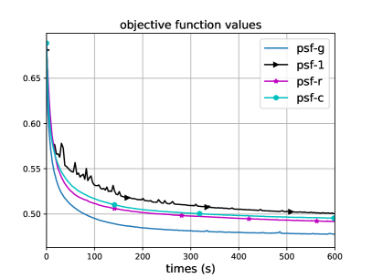
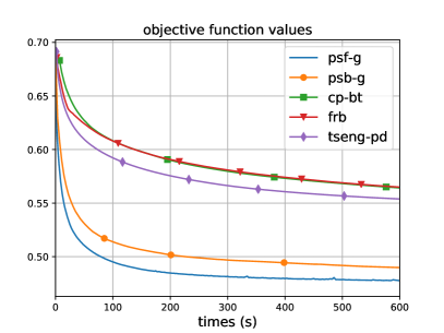
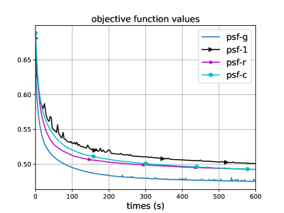
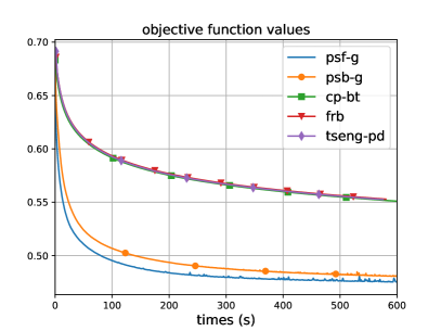
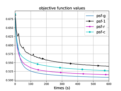
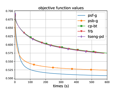
Figure 2: Objective values against wall-clock running time. Top row: $\lambda=10^{-8}$, middle row: $\lambda=10^{-6}$, bottom row: $\lambda=10^{-4}$.

- (1) Alotaibi, A., Combettes, P.L., Shahzad, N.: Solving coupled composite monotone inclusions by successive Fejér approximations of their Kuhn-Tucker set. SIAM Journal on Optimization 24(4), 2076–2095 (2014)
- (2) Bauschke, H.H., Combettes, P.L.: Convex analysis and monotone operator theory in Hilbert spaces, 2nd edn. Springer (2017)
- (3) Beck, A., Teboulle, M.: Fast gradient-based algorithms for constrained total variation image denoising and deblurring problems. IEEE Transactions on Image Processing 18(11), 2419–2434 (2009)
- (4) Boyd, S., Parikh, N., Chu, E., Peleato, B., Eckstein, J.: Distributed optimization and statistical learning via the alternating direction method of multipliers. Foundations and Trends in Machine Learning 3(1), 1–122 (2011)
- (5) Briceño-Arias, L.M., Combettes, P.L.: A monotone+ skew splitting model for composite monotone inclusions in duality. SIAM Journal on Optimization 21(4), 1230–1250 (2011)
- (6) Chambolle, A., Pock, T.: A first-order primal-dual algorithm for convex problems with applications to imaging. Journal of Mathematical Imaging and Vision 40(1), 120–145 (2011)
- (7) Combettes, P.L.: Fejér monotonicity in convex optimization. In: Encyclopedia of optimization, vol. 2, pp. 106–114. Springer Science & Business Media (2001)
- (8) Combettes, P.L., Eckstein, J.: Asynchronous block-iterative primal-dual decomposition methods for monotone inclusions. Mathematical Programming 168(1-2), 645–672 (2018)
- (9) Combettes, P.L., Pesquet, J.C.: Proximal splitting methods in signal processing. In: Fixed-point algorithms for inverse problems in science and engineering, pp. 185–212. Springer (2011)
- (10) Combettes, P.L., Pesquet, J.C.: Primal-dual splitting algorithm for solving inclusions with mixtures of composite, Lipschitzian, and parallel-sum type monotone operators. Set-Valued and variational analysis 20(2), 307–330 (2012)
- (11) Combettes, P.L., Vũ, B.C.: Variable metric forward–backward splitting with applications to monotone inclusions in duality. Optimization 63(9), 1289–1318 (2014)
- (12) Combettes, P.L., Wajs, V.R.: Signal recovery by proximal forward-backward splitting. Multiscale Modeling & Simulation 4(4), 1168–1200 (2005)
- (13) Condat, L.: A primal–dual splitting method for convex optimization involving Lipschitzian, proximable and linear composite terms. Journal of Optimization Theory and Applications 158(2), 460–479 (2013)
- (14) Davis, D., Yin, W.: A three-operator splitting scheme and its optimization applications. Set-Valued and Variational Analysis 25(4), 829––858 (2017)
- (15) Eckstein, J.: A simplified form of block-iterative operator splitting and an asynchronous algorithm resembling the multi-block alternating direction method of multipliers. Journal of Optimization Theory and Applications 173(1), 155–182 (2017)
- (16) Eckstein, J., Svaiter, B.F.: A family of projective splitting methods for the sum of two maximal monotone operators. Mathematical Programming 111(1), 173–199 (2008)
- (17) Eckstein, J., Svaiter, B.F.: General projective splitting methods for sums of maximal monotone operators. SIAM Journal on Control and Optimization 48(2), 787–811 (2009)
- (18) Eckstein, J., Yao, W.: Approximate ADMM algorithms derived from Lagrangian splitting. Computational Optimization and Applications 68(2), 363–405 (2017)
- (19) Eckstein, J., Yao, W.: Relative-error approximate versions of Douglas-Rachford splitting and special cases of the ADMM. Math. Program. 170(2), 417–444 (2018)
- (20) Iusem, A., Svaiter, B.: A variant of Korpelevich’s method for variational inequalities with a new search strategy. Optimization 42(4), 309–321 (1997)
- (21) Johnstone, P.R., Eckstein, J.: Convergence rates for projective splitting. SIAM Journal on Optimization 29(3), 1931–1957 (2019)
- (22) Komodakis, N., Pesquet, J.C.: Playing with duality: An overview of recent primal-dual approaches for solving large-scale optimization problems. IEEE Signal Processing Magazine 32(6), 31–54 (2015)
- (23) Korpelevich, G.: The extragradient method for finding saddle points and other problems. Matecon 12, 747–756 (1976)
- (24) Krasnosel’skii, M.A.: Two remarks on the method of successive approximations. Uspekhi Matematicheskikh Nauk 10(1), 123–127 (1955)
- (25) Lions, P.L., Mercier, B.: Splitting algorithms for the sum of two nonlinear operators. SIAM Journal on Numerical Analysis 16(6), 964–979 (1979)
- (26) Malitsky, Y., Pock, T.: A first-order primal-dual algorithm with linesearch. SIAM Journal on Optimization 28(1), 411–432 (2018)
- (27) Malitsky, Y., Tam, M.K.: A forward-backward splitting method for monotone inclusions without cocoercivity. arXiv preprint arXiv:1808.04162 (2018)
- (28) Mann, W.R.: Mean value methods in iteration. Proceedings of the American Mathematical Society 4(3), 506–510 (1953)
- (29) Mercier, B., Vijayasundaram, G.: Lectures on topics in finite element solution of elliptic problems. Tata Institute of Fundamental Research, Bombay (1979)
- (30) Nocedal, J.: Updating quasi-Newton matrices with limited storage. Math. Comp. 35(151), 773–782 (1980)
- (31) Pedregosa, F., Gidel, G.: Adaptive three operator splitting. Tech. Rep. 1804.02339, arXiv (2018)
- (32) Solodov, M.V., Svaiter, B.F.: A hybrid projection-proximal point algorithm. Journal of convex analysis 6(1), 59–70 (1999)
- (33) Solodov, M.V., Svaiter, B.F.: A new projection method for variational inequality problems. SIAM Journal on Control and Optimization 37(3), 765–776 (1999)
- (34) Tran-Dinh, Q., Vũ, B.C.: A new splitting method for solving composite monotone inclusions involving parallel-sum operators. Preprint 1505.07946, arXiv (2015)
- (35) Tseng, P.: A modified forward-backward splitting method for maximal monotone mappings. SIAM Journal on Control and Optimization 38(2), 431–446 (2000)
- (36) Vũ, B.C.: A splitting algorithm for dual monotone inclusions involving cocoercive operators. Advances in Computational Mathematics 38(3), 667–681 (2013)
- (37) Vũ, B.C.: A variable metric extension of the forward–backward–forward algorithm for monotone operators. Numerical Functional Analysis and Optimization 34(9), 1050–1065 (2013)
- (38) Yan, X., Bien, J.: Rare Feature Selection in High Dimensions. arXiv preprint arXiv:1803.06675 (2018)