Polyglot Semantic Parsing in APIs

Abstract

Traditional approaches to semantic parsing (SP) work by training individual models for each available parallel dataset of text-meaning pairs. In this paper, we explore the idea of polyglot semantic translation, or learning semantic parsing models that are trained on multiple datasets and natural languages. In particular, we focus on translating text to code signature representations using the software component datasets of Richardson and Kuhn (2017a, b). The advantage of such models is that they can be used for parsing a wide variety of input natural languages and output programming languages, or mixed input languages, using a single unified model. To facilitate modeling of this type, we develop a novel graph-based decoding framework that achieves state-of-the-art performance on the above datasets, and apply this method to two other benchmark SP tasks.

1 Introduction

Recent work by Richardson and Kuhn (2017a, b); Miceli Barone and Sennrich (2017) considers the problem of translating source code documentation to lower-level code template representations as part of an effort to model the meaning of such documentation. Example documentation for a number of programming languages is shown in Figure 1, where each docstring description in red describes a given function (blue) in the library. While capturing the semantics of docstrings is in general a difficult task, learning the translation from descriptions to formal code representations (e.g., formal representations of functions) is proposed as a reasonable first step towards learning more general natural language understanding models in the software domain. Under this approach, one can view a software library, or API, as a kind of parallel translation corpus for studying $\emph{text}\to\texttt{code}$ or $\texttt{code}\to\emph{text}$ translation.

1. ($en$, Java) Documentation *Returns the greater of two long values
public static long max(long a, long b)

2. ($en$, Python) Documentation

max(self, a, b): 

     ”””Compares two values numerically 

     and returns the maximum””” 

3. ($en$, Haskell) Documentation

--| ”The largest element of a non-empty structure” 

maximum :: forall z. Ord a a => t a -> a 

4. ($de$, PHP) Documentation *gibt den größeren dieser Werte zurück.
max (mixed $value1, mixed $value2)


Figure 1: Example source code documentation.

Richardson and Kuhn (2017b) extracted the standard library documentation for 10 popular programming languages across a number of natural languages to study the problem of text to function signature translation. Initially, these datasets were proposed as a resource for studying semantic parser induction Mooney (2007), or for building models that learn to translate text to formal meaning representations from parallel data. In follow-up work Richardson and Kuhn (2017a), they proposed using the resulting models to do automated question-answering (QA) and code retrieval on target APIs, and experimented with an additional set of software datasets built from 27 open-source Python projects.

As traditionally done in SP Zettlemoyer and Collins (2012), their approach involves learning individual models for each parallel dataset or language pair, e.g., ($en$, Java), ($de$, PHP), and ($en$, Haskell). Looking again at Figure 1, we notice that while programming languages differ in terms of representation conventions, there is often overlap between the functionality implemented and naming in these different languages (e.g., the max function), and redundancy in the associated linguistic descriptions. In addition, each English description (Figure 1.1-1.3) describes max differently using the synonyms greater, maximum, largest. In this case, it would seem that training models on multiple datasets, as opposed to single language pairs, might make learning more robust, and help to capture various linguistic alternatives.

With the software QA application in mind, an additional limitation is that their approach does not allow one to freely translate a given description to multiple output languages, which would be useful for comparing how different programming languages represent the same functionality. The model also cannot translate between natural languages and programming languages that are not observed during training. While software documentation is easy to find in bulk, if a particular API is not already documented in a language other than English (e.g., Haskell in $de$), it is unlikely that such a translation will appear without considerable effort by experienced translators. Similarly, many individual APIs may be too small or poorly documented to build individual models or QA applications, and will in some way need to bootstrap off of more general models or resources.

To deal with these issues, we aim to learn more general text-to-code translation models that are trained on multiple datasets simultaneously. Our ultimate goal is to build polyglot translation models (cf. Johnson et al. (2016)), or models with shared representations that can translate any input text to any output programming language, regardless of whether such language pairs were encountered explicitly during training. Inherent in this task is the challenge of building an efficient polyglot decoder, or a translation mechanism that allows such crossing between input and output languages. A key challenge is ensuring that such a decoder generates well-formed code representations, which is not guaranteed when one simply applies standard decoding strategies from SMT and neural MT (cf. Cheng et al. (2017)). Given our ultimate interest in API QA, such a decoder must also facilitate monolingual translation, or being able to translate to specific output languages as needed.

To solve the decoding problem, we introduce a new graph-based decoding and representation framework that reduces to solving shortest path problems in directed graphs. We investigate several translation models that work within this framework, including traditional SMT models and models based on neural networks, and report state-of-the-art results on the technical documentation task of Richardson and Kuhn (2017b, a). To show the applicability of our approach to more conventional SP tasks, we apply our methods to the GeoQuery domain Zelle and Mooney (1996) and the Sportscaster corpus Chen et al. (2010). These experiments also provide insight into the main technical documentation task and highlight the strengths and weaknesses of the various translation models being investigated.

2 Related Work

Our approach builds on the baseline models introduced in Richardson and Kuhn (2017b) (see also Deng and Chrupała (2014)). Their work is positioned within the broader SP literature, where traditionally SMT Wong and Mooney (2006a) and parsing Zettlemoyer and Collins (2009) methods are used to study the problem of translating text to formal meaning representations, usually centering around QA applications Berant et al. (2013). More recently, there has been interest in using neural network approaches either in place of Dong and Lapata (2016); Kočiský et al. (2016) or in combination with Misra and Artzi (2016); Jia and Liang (2016); Cheng et al. (2017) these traditional models, the latter idea we look at in this paper.

Work in NLP on software documentation has accelerated in recent years due in large part to the availability of new data resources through websites such as StackOverflow and Github (cf. Allamanis et al. (2017)). Most of this recent work focuses on processing large amounts of API data in bulk Gu et al. (2016); Miceli Barone and Sennrich (2017), either for learning longer executable programs from text Yin and Neubig (2017); Rabinovich et al. (2017), or solving the inverse problem of code to text generation Iyer et al. (2016); Richardson et al. (2017). In contrast to our work, these studies do not look explicitly at translating to target APIs, or at non-English documentation.

The idea of polyglot modeling has gained some traction in recent years for a variety of problems Tsvetkov et al. (2016) and has appeared within work in SP under the heading of multilingual SP Jie and Lu (2014); Duong et al. (2017). A related topic is learning from multiple knowledge sources or domains Herzig and Berant (2017), which is related to our idea of learning from multiple APIs. When building models that can translate between unobserved language pairs, we use the term zero-shot translation from Johnson et al. (2016).

3 Baseline Semantic Translator

Problem Formulation

Throughout the paper, we refer to target code representations as API components. In all cases, components will consist of formal representations of functions, or function signatures (e.g., long max(int a, int b)), which include a function name (max), a sequence of arguments (int a, int b), and other information such as a return value (long) and namespace (for more details, see Richardson (2018)). For a given API dataset $D=\{(\textbf{x}_{i},\textbf{z}_{i})\}_{i=1}^{n}$ of size $n$, the goal is to learn a model that can generate exactly a correct component sequence $\textbf{z}=(z_{1},..,z_{|\textbf{z}|})$, within a finite space $\mathcal{C}$ of signatures (i.e., the space of all defined functions), for each input text sequence $\textbf{x}=(x_{1},...,x_{|\textbf{x}|})$. This involves learning a probability distribution $p(\textbf{z}\mid\textbf{x})$. As such, one can think of this underlying problem as a constrained MT task.

In this section, we describe the baseline approach of Richardson and Kuhn (2017b). Technically, their approach has two components: a simple word-based translation model and task specific decoder, which is used to generate a $k$-best list of candidate component representations for a given input x. They then use a discriminative model to rerank the translation output using additional non-world level features. The goal in this section is to provide the technical details of their translation approach, which we improve in Section 4.

3.1 Word-based Translation Model

The translation models investigated in Richardson and Kuhn (2017b) use a noisy-channel formulation where $p(\textbf{z}\mid\textbf{x})\propto p(\textbf{x}\mid\textbf{z})p(\textbf{z})$ via Bayes rule. By assuming a uniform prior on output components, $p(\textbf{z})$, the model therefore involves estimating $p(\textbf{x}\mid\textbf{z})$, which under a word-translation model is computed using the following formula: $p(\textbf{x}\mid\textbf{z})=\sum_{a\in\mathcal{A}}p(\textbf{x},a\mid\textbf{z})$, where the summation ranges over the set of all many-to-one word alignments $\mathcal{A}$ from $\textbf{x}\to\textbf{z}$, with $|\mathcal{A}|$ equal to $(|\textbf{z}|+1)^{|\textbf{x}|}$. They investigate various types of sequence-based alignment models Och and Ney (2003), and find that the classic IBM Model 1 outperforms more complex word models. This model factors in the following way and assumes an independent word generation process:

$$p(\textbf{x}\mid\textbf{z})=\frac{1}{|\mathcal{A}|}\prod_{j=1}^{|\textbf{x}|}\sum_{i=0}^{|\textbf{z}|}p_{t}(x_{j}\mid z_{i})$$ (1)

where each $p_{t}$ defines a multinomial distribution over a given component term $z$ for all words $x$.

The decoding problem for the above translation model involves finding the most likely output $\hat{z}$, which requires solving an $\operatorname*{arg\,max}_{\textbf{z}}$ over Equation 1. In the general case, this problem is known to be $\mathcal{NP}$-complete for the models under consideration Knight (1999) largely due to the large space of possible predictions z. Richardson and Kuhn (2017b) avoid these issues by exploiting the finiteness of the target component search space (an idea we also pursue here and discuss more below), and describe a constrained decoding algorithm that runs in time $O(|\mathcal{C}|\log|\mathcal{C}|)$. While this works well for small APIs, it becomes less feasible when dealing with large sets of APIs, as in the polyglot case, or with more complex semantic languages typically used in SP Liang (2013).

Figure 2: A DAFSA representation for a portion of the component sequence search space $\mathcal{C}$ that includes math functions in C and Clojure, and an example path/translation (in bold): 2C numeric math ceil arg.

4 Shortest Path Framework

To improve the baseline translation approach used previously (Section 3.1), we pursue a graph based approach. Given the formulation above and the finiteness of our prediction space $\mathcal{C}$, our approach exploits the fact that we can represent the complete component search space for any set of APIs as a directed acyclic finite-state automaton (DAFSA), such as the one shown graphically in Figure 2. The underlying graph is constructed by concatenating all of the component representations for each API of interest and applying standard finite-state construction and minimization techniques Mohri (1996). Each path in the resulting compact automaton is therefore a well-formed component representation.

Using an idea from Johnson et al. (2016), we add to each component representation an artificial token that identifies the output programming language or library. For example, the two edges from the initial state $0$ in Figure 2 are labeled as 2C and 2Clojure, which identify the C and Clojure programming languages respectively. All paths starting from the right of these edges are therefore valid paths in each respective programming language. The paths starting from the initial state $0$, in contrast, correspond to all valid component representations in all languages.

Decoding reduces to the problem of finding a path for a given text input x. For example, given the input the ceiling of a number, we would want to find the paths corresponding to the component translations numeric math ceil arg (in C) and algo math ceil x (in Clojure) in the graph shown in Figure 2. Using the trick above, our setup facilitates both monolingual decoding, i.e., generating components specific to a particular output language (e.g., the C language via the path shown in bold), and polyglot decoding, i.e., generating any output language by starting at the initial state 0 (e.g., C and Clojure).

We formulate the decoding problem using a variant of the well-known single source shortest path (SSSP) algorithm for directed acyclic graphs (DAGs) (Johnson (1977)). This involves a graph $\mathcal{G}=(V,E)$ (nodes $V$ and labeled edges $E$, see graph in Figure 2), and taking an off-line topological sort of the graph’s vertices. Using a data structure $d\in\mathbb{R}^{|V|}$ (initialized as $\infty^{|V|}$, as shown in Figure 2), the standard SSSP algorithm (which is the forward update variant of the Viterbi algorithm Huang (2008)) works by searching forward through the graph in sorted order and finding for each node $v$ an incoming labeled edge $u$, with label $z$, that solves the following recurrence:

$$d(v)=\underset{(u,z):(u,v,z)\in E}{\min}\Big{\{}d(u)+w(u,v,z)\Big{\}}$$ (2)

where $d(u)$ is shortest path score from a unique source node $b$ to the incoming node $u$ (computed recursively) and $w(u,v,z)$ is the weight of the particular labeled edge. The weight of the resulting shortest path is commonly taken to be the sum of the path edge weights as given by $w$, and the output translation is the sequence of labels associated with each edge. This algorithm runs in linear time over the size of the graph’s adjacency matrix (Adj) and can be extended to find $k$ SSSPs. In the standard case, a weighting function $w$ is provided by assuming a static weighted graph. In our translation context, we replace $w$ with a translation model, which is used to dynamically generate edge weights during the SSSP search for each input x by scoring the translation between x and each edge label $z$ encountered.

Given this general framework, many different translation models can be used for scoring. In what follows, we describe two types of decoders based on lexical translation (or unigram) and neural sequence models. Technically, each decoding algorithm involves modifying the standard SSSP search procedure by adding an additional data structure $s$ to each node (see Figure 2), which is used to store information about translations (e.g., running lexical translation scores, RNN state information) associated with particular shortest paths. By using these two very different models, we can get insight into the challenges associated with the technical documentation translation task. As we show in Section 6, each model achieves varying levels of success when subjected to a wider range of SP tasks, which reveals differences between our task and other SP tasks.

4.1 Lexical Translation Shortest Path

Algorithm 1 Lexical Shortest Path Search

1:Input x of size $n$, DAG $\mathcal{G}=(V,E)$, lexical translation function $p_{t}$, source node $b$ with initial score $o$.

2:Shortest component path

3:$d[V[\mathcal{G}]]\leftarrow\infty,\pi[V[\mathcal{G}]]\leftarrow Nil,d[b]\leftarrow o$

4:$s[V[\mathcal{G}],n]\leftarrow 0.0$$\triangleright$ Shortest path sums at each node

5:for each vertex $u\geq b\in V[\mathcal{G}]$ in sorted order  do

6:     for each vertex and label $(v,z)\in\texttt{Adj}[u]$ do

7:         $\texttt{score}\leftarrow-log\big{[}\thinspace\thinspace\prod_{i}^{n}p_{t}(x_{i}\mid z)+s[u,i]$   ]

8:         if $d[v]>\texttt{score}$ then

9:              $d[v]\leftarrow\texttt{score},\pi[v]\leftarrow u$

10:              for $i$ in $1,..,n$ do$\triangleright$ Update scores

11:                  $s[v,i]\leftarrow p_{t}(x_{i}\mid z)+s[u,i]$                             

12:return FindPath$(\pi,|V|,b)$

In our first model, we use the lexical translation model and probability function $p_{t}$ in Equation 1 as the weighting function, which can be learned efficiently off-line using the EM algorithm. When attempting to use the SSSP procedure to compute this equation for a given source input x, we immediately have the problem that such a computation requires a complete component representation z Knight and Al-Onaizan (1998). We use an approximation that involves ignoring the normalizer $|\mathcal{A}|$ and exploiting the word independence assumption of the model, which allows us to incrementally compute translation scores for individual source words given output translations corresponding to shortest paths during the SSSP search.

The full decoding algorithm in shown in Algorithm 1, where the red highlights the adjustments made to the standard SSSP search as presented in Cormen et al. (2009). The main modification involves adding a data structure $s\in\mathbb{R}^{|V|\thinspace\times\thinspace|\textbf{x}|}$ (initialized as $0.0^{|V|\times|\textbf{x}|}$ at line 2) that stores a running sum of source word scores given the best translations at each node, which can be used for computing the inner sum in Equation 1. For example, given an input utterance ceiling function, $s_{6}$ in Figure 2 contains the independent translation scores for words ceiling and function given the edge label numeric and $p_{t}$. Later on in the search, these scores are used to compute $s_{7}$, which will provide translation scores for each word given the edge sequence numeric math. Taking the product over any given $s_{j}$ (as done in line 7 to get score) will give the probability of the shortest path translation at the particular point $j$. Here, the transformation into $-\log$ space is used to find the minimum incoming path. Standardly, the data structure $\pi$ can be used to retrieve the shortest path back to the source node $b$ (done via the FindPath method).

4.2 Neural Shortest Path

Our second set of models use neural networks to compute the weighting function in Equation 2. We use an encoder-decoder model with global attention Bahdanau et al. (2014); Luong et al. (2015), which has the following two components:

Encoder Model

The first is an encoder network, which uses a bi-directional recurrent neural network architecture with LSTM units Hochreiter and Schmidhuber (1997) to compute a sequence of forward annotations or hidden states $(\overrightarrow{h}_{1},...,\overrightarrow{h}_{|\textbf{x}|})$ and a sequence of backward hidden states $(\overleftarrow{h},...,\overleftarrow{h}_{|\textbf{x}|})$ for the input sequence $(x_{1},...,x_{|\textbf{x}|})$. Standardly, each word is then represented as the concatenation of its forward and backward states: $h_{j}=[\overrightarrow{h}_{j},\overleftarrow{h}_{j}]$.

Decoder Model

The second component is a decoder network, which directly computes the conditional distribution $p(\textbf{z}\mid\textbf{x})$ as follows:

$$p(\textbf{z}\mid\textbf{x})=\sum_{i=1}^{|\textbf{z}|}\log p_{\Theta}(z_{i}\mid z_{<i},\textbf{x})$$ (3)

$$p_{\Theta}(z_{i}\mid z_{<i},\textbf{x})\sim\texttt{softmax}(f(\Theta,z_{<i},\textbf{x}))$$ (4)

where $f$ is a non-linear function that encodes information about the sequence $z_{<i}$ and the input x given the model parameters $\Theta$. We can think of this model as an ordinary recurrent language model that is additionally conditioned on the input x using information from our encoder. We implement the function $f$ in the following way:

$$f(\Theta,z_{<i},\textbf{x})=\textbf{W}_{o}\eta_{i}+\textbf{b}_{o}$$ (5)

$$\eta_{i}=\texttt{MLP}(c_{i},g_{i})$$ (6)

$$g_{i}=\texttt{LSTM}_{dec}(g_{i-1},\textbf{E}^{out}_{z_{i-1}},c_{i})$$ (7)

where MLP is a multi-layer perceptron model with a single hidden layer, $\textbf{E}^{out}\in\mathbb{R}^{|\Sigma_{dec}|\times e}$ is a randomly initialized embedding matrix, $g_{i}$ is the decoder’s hidden state at step $i$, and $c_{i}$ is a context-vector that encodes information about the input x and the encoder annotations. Each context vector $c_{i}$ in turn is a weighted sum of each annotation $h_{j}$ against an attention vector $\alpha_{i,j}$, or $c_{i}=\sum_{j=1}^{|\textbf{x}|}\alpha_{i,j}h_{j}$, which is jointly learned using an additional single layered multi-layer perceptron defined in the following way:

$$\alpha_{i,j}\propto\exp(e_{i,j});\quad e_{i,j}=\texttt{MLP}(g_{i-1},h_{j})$$ (8)

Lexical Bias and Copying

In contrast to standard MT tasks, we are dealing with a relatively low-resource setting where the sparseness of the target vocabulary is an issue. For this reason, we experimented with integrating lexical translation scores using a biasing technique from Arthur et al. (2016). Their method is based on the following computation for each token $z_{i}$:

$$\texttt{bias}_{i}=\quad\quad\quad\quad\quad\quad\quad\quad\quad\quad\quad\quad\quad\quad\quad\quad$$

$$\begin{bmatrix}p_{t^{\prime}}(z_{1}\mid x_{1})&\dots&p_{t^{\prime}}(z_{1}\mid x_{|\textbf{x}|})\\ \vdots&\ddots&\vdots\\ p_{t^{\prime}}(z_{\mid\Sigma_{dec}\mid}\mid x_{1})&\dots&p_{t^{\prime}}(z_{\mid\Sigma_{dec}\mid}\mid x_{|\textbf{x}|})\end{bmatrix}\begin{bmatrix}\alpha_{i,1}\\ \vdots\\ \alpha_{i,\mid\textbf{x}\mid}\end{bmatrix}$$

The first matrix uses the inverse ($p_{t^{\prime}}$) of the lexical translation function $p_{t}$ already introduced to compute the probability of each word in the target vocabulary $\Sigma_{dec}$ (the columns) with each word in the input x (the rows), which is then weighted by the attention vector from Equation 8. $bias_{i}$ is then used to modify Equation 5 in the following way:

$$f_{bias}(\Theta,z_{<i},\textbf{x})={} \textbf{W}_{o}\eta_{i}+\textbf{b}_{o}+$$

$$\log(\texttt{bias}_{i}+\epsilon)$$

where $\epsilon$ is a hyper-parameter that helps to preserve numerical stability and biases more heavily on the lexical model when set lower.

We also experiment with the copying mechanism from Jia and Liang (2016), which works by allowing the decoder to choose from a set of latent actions, $a_{j}$, that includes writing target words according to Equation 5, as done standardly, or copying source words from x, or $\texttt{copy}[x_{i}]$ according to the attention scores in Equation 8. A distribution is then computed over these actions using a softmax function and particular actions are chosen accordingly during training and decoding.

Algorithm 2 Neural Shortest Path Search

1:Input x, DAG $\mathcal{G}$, neural parameters $\Theta$ and non-linear function $f$, beam size $l$, source node $b$ with init. score $o$.

2:Shortest component path

3:$d[V[\mathcal{G}]]\leftarrow\infty,d[b]\leftarrow o,\pi[V[\mathcal{G}]]\leftarrow Nil$

4:$s[V[\mathcal{G}]]\leftarrow Nil$$\triangleright$ Path state information

5:$s[b]\leftarrow\texttt{InitState()}$$\triangleright$ Initialize source state

6:for each vertex $u\geq b\in V[\mathcal{G}]$ in sorted order  do

7:     if $\texttt{isinf}(d[u])$ then continue      

8:     $p\leftarrow s[u]$$\triangleright$ Current state at node $u$, or $z_{<i}$

9:     $L^{1}_{[l]}\leftarrow\underset{(v_{1},...,v_{k})\in\texttt{Adj}[u]}{\operatorname*{arg\,max}}{\texttt{softmax}(f(\Theta,p,\textbf{x})})$

10:     for each vertex and label $(v,z)\in L$ do

11:         score $\leftarrow-\log p_{\Theta}(z\mid p,\textbf{x})+d[u]$

12:         if $d[v]>\texttt{score}$ then

13:              $d[v]\leftarrow\texttt{score},\pi[v]\leftarrow u$

14:              $s[v]\leftarrow\texttt{UpdateState}(p,z)$               

15:return FindPath$(\pi,|V|,b)$

Decoding and Learning

The full decoding procedure is shown in Algorithm 2, where the differences with the standard SSSP are again shown in red. We change the data structure $s$ to contain the decoder’s RNN state at each node. We also modify the scoring (line 7, which uses Equation 4) to consider only the top $l$ edges or translations at that point, as opposed to imposing a full search. When $l$ is set to 1, for example, the procedure does a greedy search through the graph, whereas when $l$ is large the procedure is closer to a full search.

In general terms, the decoder described above works like an ordinary neural decoder with the difference that each decision (i.e., new target-side word translation) is constrained (in line 7) by the transitions allowed in the underlying graph in order to ensure wellformedness of each component output. Standardly, we optimize these models using stochastic gradient descent with the objective of finding parameters $\hat{\Theta}$ that minimize the negative conditional log-likelihood of the training dataset.

4.3 Monolingual vs. Polyglot Decoding

Our framework facilitates both monolingual and polyglot decoding. In the first case, the decoder requires a graph associated with the output semantic language (more details in next section) and a trained translation model. The latter case requires taking the union of all datasets and graphs (with artificial identifier tokens) for a collection of target datasets and training a single model over this global dataset. In this setting, we can then decode to a particular language using the language identifiers or decode without specifying the output language. The main focus in this paper is investigating polyglot decoding, and in particular the effect of training models on multiple datasets when translating to individuals APIs or SP datasets.

When evaluating our models and building QA applications, it is important to be able to generate the $k$ best translations. This can easily be done in our framework by applying standard $k$ SSSP algorithms Brander and Sinclair (1995). We use an implementation of the algorithm of Yen (1971), which works on top of the SSSP algorithms introduced above by iteratively finding deviating or branching paths from an initial SSSP (more details provided in supplementary materials).

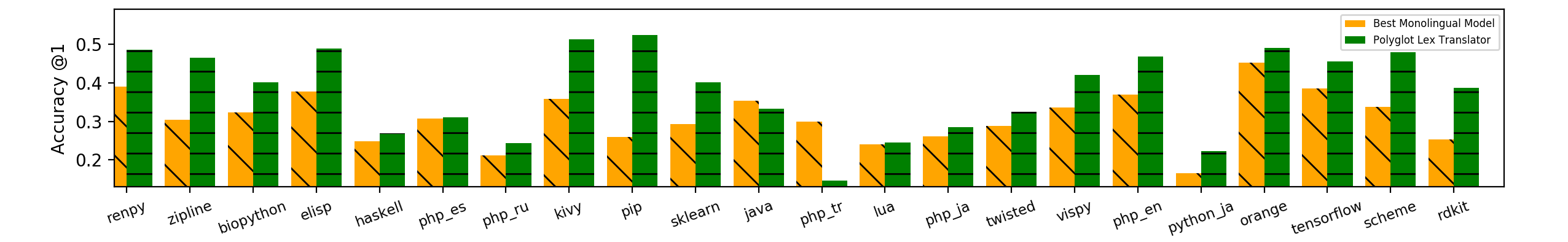
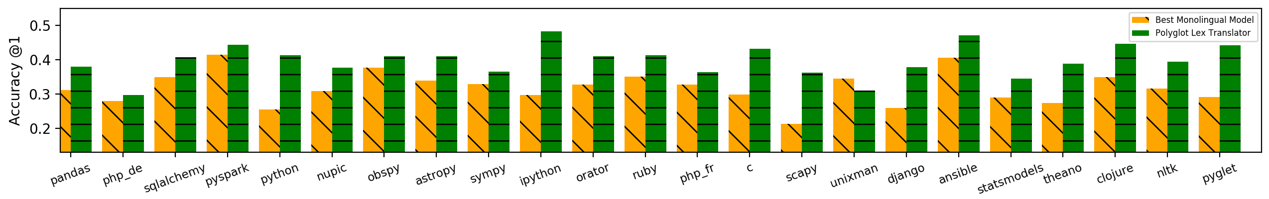
Figure 3: Test Acc@1 for the best monolingual models (in yellow/left) compared with the best lexical polyglot model (green/right) across all 45 technical documentation datasets.

5 Experiments

We experimented with two main types of resources: 45 API documentation datasets and two multilingual benchmark SP datasets. In the former case, our main objective is to test whether training polyglot models (shown as polyglot in Tables 1-2) on multiple datasets leads to an improvement when compared to training individual monolingual models (shown as monolingual in Tables 1-2). Experiments involving the latter datasets are meant to test the applicability of our general graph and polyglot method to related SP tasks, and are also used for comparison against our main technical documentation task.

5.1 Datasets

Technical API Docs

The first dataset includes the Stdlib and Py27 datasets of Richardson and Kuhn (2017b, a), which are publicly available via Richardson (2017). Stdlib consists of short description and function signature pairs for 10 programming languages in 7 languages, and Py27 contains the same type of data for 27 popular Python projects in English mined from Github. We also built new datasets from the Japanese translation of the Python 2.7 standard library, as well as the Lua stdlib documentation in a mixture of Russian, Portuguese, German, Spanish and English.

Taken together, these resources consist of 79,885 training pairs, and we experiment with training models on Stdlib and Py27 separately as well as together (shown as + more in Table 1). We use a BPE subword encoding (Sennrich et al., 2015) of both input and output words to make the representations more similar and transliterated all datasets (excluding Japanese datasets) to an 8-bit latin encoding. Graphs were built by concatenating all function representations into a single word list and compiling this list into a minimized DAFSA. For our global polyglot dataset, this resulted in a graph with 218,505 nodes, 313,288 edges, and 112,107 paths or component representations over an output vocabulary of 9,324 words.

Mixed GeoQuery and Sportscaster

We run experiments on the GeoQuery 880 corpus using the splits from Andreas et al. (2013), which includes geography queries for English, Greek, Thai, and German paired with formal database queries, as well as a seed lexicon or NP list for each language. In addition to training models on each individual dataset, we also learn polyglot models trained on all datasets concatenated together. We also created a new mixed language test set that was built by replacing NPs in 803 test examples with one or more NPs from a different language using the NP lists mentioned above (see examples in Figure 4). The goal in the last case is to test our model’s ability to handle mixed language input. We also ran monolingual experiments on the English Sportscaster corpus, which contains human generated soccer commentary paired with symbolic meaning representation produced by a simulation of four games.

For GeoQuery graph construction, we built a single graph for all languages by extracting general rule templates from all representations in the dataset, and exploited additional information and patterns using the Geobase database and the semantic grammars used in Wong and Mooney (2006b). This resulted in a graph with 2,419 nodes, 4,936 edges and 39,482 paths over an output vocabulary of 164. For Sportscaster, we directly translated the semantic grammar provided in Chen and Mooney (2008) to a DAFSA, which resulted in a graph with 98 nodes, 86 edges and 830 paths.

5.2 Experimental Setup

For the technical datasets, the goal is to see if our model generates correct signature representations from unobserved descriptions using exact match. We follow exactly the experimental setup and data splits from Richardson and Kuhn (2017b), and measure the accuracy at 1 (Acc@1), accuracy in top 10 (Acc@10), and MRR.

For the GeoQuery and Sportscaster experiments, the goal is to see if our models can generate correct meaning representations for unseen input. For GeoQuery, we follow Andreas et al. (2013) in evaluating extrinsically by checking that each representation evaluates to the same answer as the gold representation when executed against the Geobase database. For Sportscaster, we evaluate by exact match to a gold representation.

		Method	Acc@1	Acc@10	MRR
stdlib	mono.	RK Trans + rerank	29.9	69.2	43.1
2-6		Lexical SP	33.2	70.7	45.9
	poly.	Lexical SP + more	33.1	69.7	45.5
3-6		Neural SP + bias	12.1	34.3	19.5
		Neural SP + copy_bias	13.9	36.5	21.5
py27	mono.	RK Trans + rerank	32.4	73.5	46.5
2-6		Lexical SP	41.3	77.7	54.1
	poly.	Lexical SP + more	40.5	76.7	53.1
3-6		Neural SP + bias	8.7	25.5	14.2
		Neural SP + copy_bias	9.0	26.9	15.1

Table 1: Test results on the Stdlib and Py27 tasks averaged over all datasets and compared against the best monolingual results from Richardson and Kuhn (2017b, a), or RK

5.3 Implementation and Model Details

We use the Foma finite-state toolkit of Hulden (2009) to construct all graphs used in our experiments. We also use the Cython version of Dynet Neubig et al. (2017) to implement all the neural models (see supp. materials for more details).

In the results tables, we refer to the lexical and neural models introduced in Section 4 as Lexical Shortest Path and Neural Shortest Path, where models that use copying (+ copy) and lexical biasing (+ bias) are marked accordingly. We also experimented with adding a discriminative reranker to our lexical models (+ rerank), using the approach from Richardson and Kuhn (2017b), which uses additional lexical (e.g., word match and alignment) features and other phrase-level and syntax features. The goal here is to see if these additional (mostly non-word level) features help improve on the baseline lexical models.

6 Results and Discussion

		Method	Acc@1	Acc@10
		UBL Kwiatkowski et al. (2010)	74.2	–
		TreeTrans Jones et al. (2012)	76.8	–
		nHT Susanto and Lu (2017)	83.3	–
3-6 Standard Geoquery	monolingual	Lexical Shortest Path	68.6	92.4
		Lexical Shortest Path + rerank	74.2	94.1
3-6		Neural Shortest Path	73.5	91.1
		Neural Shortest Path + bias	78.0	92.8
		Neural Shortest Path + copy_bias	77.8	92.1
	polyglot	Lexical Shortest Path	67.3	92.9
		Lexical Shortest Path + rerank	75.2	94.7
3-6		Neural Shortest Path	78.0	91.4
		Neural Shortest Path + bias	78.9	91.7
		Neural Shortest Path + copy_bias	79.6	91.9
1-6 Mixed	poly.	Best Monolingual Model	4.2	18.2
		Lexical Shortest Path + rerank	71.1	94.3
		Neural Shortest Path + copy_bias	75.2	90.0
	mono.	PCFG Börschinger et al. (2011)	74.2	–
		wo-PCFG Börschinger et al. (2011)	86.0	–
3-6 Sportscaster		Lexical Shortest Path	40.3	86.8
		Lexical Shortest Path + rerank	70.3	90.2
3-6		Neural Shortest Path	81.9	94.8
		Neural Shortest Path + bias	83.4	93.9
		Neural Shortest Path + copy_bias	83.3	90.5

Table 2: Test results for the standard (above) and mixed (middle) GeoQuery tasks averaged over all languages, and results for the English Sportscaster task (below).

Technical Documentation Results

Table 1 shows the results for Stdlib and Py27. In the monolingual case, we compare against the best performing models in Richardson and Kuhn (2017b, a). As summarized in Figure 3, our experiments show that training polyglot models on multiple datasets can lead to large improvements over training individual models, especially on the Py27 datasets where using a polyglot model resulted in a nearly 9% average increase in accuracy @1. In both cases, however, the best performing lexical models are those trained only on the datasets they are evaluated on, as opposed to training on all datasets (i.e., + more). This is surprising given that training on all datasets doubles the size of the training data, and shows that adding more data does not necessarily boost performance when the additional data is from another distribution.

The neural models are strongly outperformed by all other models both in the monolingual and polyglot case (only the latter results shown), even when lexical biasing is applied. While surprising, this is consistent with other studies on low-resource neural MT Zoph et al. (2016); Östling and Tiedemann (2017), where datasets of comparable size to ours (e.g., 1 million tokens or less) typically fail against classical SMT models. This result has also been found in relation to neural AMR semantic parsing, where similar issues of sparsity are encountered Peng et al. (2017). Even by doubling the amount of training data by training on all datasets (results not shown), this did not improve the accuracy, suggesting that much more data is needed (more discussion below).

Beyond increases in accuracy, our polyglot models support zero-shot translation as shown in Figure 4, which can be used for translating between unobserved language pairs (e.g., ($es$,Clojure), ($ru$,Haskell) as shown in 1-2), or for finding related functionality across different software projects (as shown in 3). These results were obtained by running our decoder model without specifying the output language. We note, however, that the decoder can be constrained to selectively translate to any specific programming language or project (e.g., in a QA setting). Future work will further investigate the decoder’s polyglot capabilities, which is currently hard to evaluate since we do not have an annotated set of function equivalences between different APIs.

1.	Source API (stdlib): (es, PHP)	Input: Devuelve el mensaje asociado al objeto lanzado.
Output	Language: PHP	Function Translation: public string Throwable::getMessage ( void )
	Language: Java	Function Translation: public String lang.getMessage( void )
	Language: Clojure	Function Translation: (tools.logging.fatal throwable message & more)
2.	Source API (stdlib): (ru, PHP)	Input: konvertiruet stroku iz formata UTF-32 v format UTF-16.
Output	Language: PHP	Function Translation: string PDF_utf32_to_utf16 ( ... )
	Language: Ruby	Function Translation: String#toutf16 => string
	Language: Haskell	Function Translation: Encoding.encodeUtf16LE :: Text -> ByteString
3.	Source API (py): (en, stats)	Input: Compute the Moore-Penrose pseudo-inverse of a matrix.
Output	Project: sympy	Function Translation: matrices.matrix.base.pinv_solve( B, ... )
	Project: sklearn	Function Translation: utils.pinvh( a, cond=None,rcond=None,... )
	Project: stats	Function Translation: tools.pinv2( a,cond=None,rcond=None )
4.	Mixed GeoQuery (de/gr)	Input: Wie hoch liegt der höchstgelegene punkt in Αλαμπάμα?
Logical Form Translation: answer(elevation_1(highest(place(loc_2(stateid(’alabama’))))))

Figure 4: Examples of zero-shot translation when running in polyglot mode (1-3, function representations shown in a conventionalized format), and mixed language parsing (4).

Semantic Parsing Results

SP results are summarized in Table 2. In contrast, the neural models, especially those with biasing and copying, strongly outperform all other models and are competitive with related work. In the GeoQuery case, we compare against two classic grammar-based models, UBL and TreeTrans, as well as a feature rich, neural hybrid tree model (nHT). We also see that the polyglot Geo achieves the best performance, demonstrating that training on multiple datasets helps in this domain as well. In the Sportscaster case we compare against two PCFG learning approaches, the second, and best performing model (wo-PCFG) involves a grammar model that encodes complex word-order constraints.

The real advantage of training a polyglot model is shown on the results related to mixed language parsing (i.e., the middle set of results). Here we compared against the best performing monolingual English model (Best Mono. Model), which clearly does not have a way to deal with multilingual NPs. We also find the neural model to be more robust than the lexical models with reranking.

While the lexical models overall perform poorly on both tasks, the weakness of this model is particularly acute in the Sportscaster case. We found that mistakes are largely related to the ordering of arguments, which these lexical (unigram) models are blind to. That these models still perform reasonably well on the Geo task shows that such ordering issues are less of a factor in this domain.

Discussion

Having results across related SP tasks allows us to reflect on the nature of the main technical documentation task. Consistent with recent findings Dong and Lapata (2016), we show that relatively simple neural sequence models are competitive with, and in some cases outperform, traditional grammar-based SP methods on benchmark SP tasks. However, this result is not observed in our technical documentation task, in part because this problem is much harder for neural learners given the sparseness of the target data and lack of redundancy. For this reason, we believe our datasets provide new challenges for neural-based SP, and serve as a cautionary tale about the scalability and applicability of commonly used neural models to lower-resource SP problems.

In general, we believe that focusing on polyglot and mixed language decoding is not only of interest to applications (e.g, mixed language API QA) but also allows for new forms of SP evaluation that are more revealing than only translation accuracy. When comparing the accuracy of the best monolingual Geo model and the worst performing neural polyglot model, one could mistakingly think that these models have equal abilities, though the polyglot model is much more robust and general. Moving forward, we hope that our work helps to motivate more diverse evaluations of this type.

7 Conclusion

In this paper, we look at learning from multiple API libraries and datasets in the context of learning to translate text to code representations and other SP tasks. To support polyglot modeling of this type, we developed a novel graph based decoding method and experimented with various SMT and neural MT models that work in this framework. We report a mixture of positive results specific to each task and set of models using this polyglot modeling idea, some of which reveal interesting limitations of different approaches to SP. We also introduced two new API datasets, and a mixed language version of Geoquery that will be released to facilitate further work on polyglot SP.

References

- Allamanis et al. (2017) Miltiadis Allamanis, Earl T Barr, Premkumar Devanbu, and Charles Sutton. 2017. A Survey of Machine Learning for Big Code and Naturalness. arXiv preprint arXiv:1709.06182 .
- Andreas et al. (2013) Jacob Andreas, Andreas Vlachos, and Stephen Clark. 2013. Semantic parsing as machine translation. In in Proceedings of ACL-2013. pages 47–52.
- Arthur et al. (2016) Philip Arthur, Graham Neubig, and Satoshi Nakamura. 2016. Incorporating Discrete Translation Lexicons into Neural Machine Translation. arXiv preprint arXiv:1606.02006 .
- Bahdanau et al. (2014) Dzmitry Bahdanau, Kyunghyun Cho, and Yoshua Bengio. 2014. Neural Machine Translation by Jointly Learning to Align and Translate. arXiv preprint arXiv:1409.0473 .
- Berant et al. (2013) Jonathan Berant, Andrew Chou, Roy Frostig, and Percy Liang. 2013. Semantic Parsing on Freebase from Question-Answer Pairs. In in Proceedings of EMNLP-2013. pages 1533–1544.
- Börschinger et al. (2011) Benjamin Börschinger, Bevan K. Jones, and Mark Johnson. 2011. Reducing grounded learning tasks to grammatical inference. In Proceedings of EMNLP-2011. pages 1416–1425.
- Brander and Sinclair (1995) AW Brander and MC Sinclair. 1995. A Comparative Study of k-Shortest Path Algorithms. In In Proc. of 11th UK Performance Engineering Workshop.
- Chen et al. (2010) David L. Chen, Joohyun Kim, and Raymond J. Mooney. 2010. Training a Multilingual Sportscaster: Using Perceptual Context to Learn Language. Journal of Artificial Intelligence Research 37:397–435.
- Chen and Mooney (2008) David L. Chen and Raymond J. Mooney. 2008. Learning to Sportscast: A Test of Grounded Language Acquisition. In Proceedings of ICML-2008. pages 128–135.
- Cheng et al. (2017) Jianpeng Cheng, Siva Reddy, Vijay Saraswat, and Mirella Lapata. 2017. Learning Structured Natural Language Representations for Semantic Parsing. arXiv preprint arXiv:1704.08387 .
- Cormen et al. (2009) T Cormen, C Leiserson, R Rivest, and C Stein. 2009. Introduction to Algorithms. MIT Press.
- Deng and Chrupała (2014) Huijing Deng and Grzegorz Chrupała. 2014. Semantic Approaches to Software Component Retrieval with English Queries. In Proceedings of LREC-14. pages 441–450.
- Dong and Lapata (2016) Li Dong and Mirella Lapata. 2016. Language to Logical Form with Neural Attention. arXiv preprint arXiv:1601.01280 .
- Duong et al. (2017) Long Duong, Hadi Afshar, Dominique Estival, Glen Pink, Philip Cohen, and Mark Johnson. 2017. Multilingual Semantic Parsing and Code-Switching. CoNLL 2017 page 379.
- Gu et al. (2016) Xiaodong Gu, Hongyu Zhang, Dongmei Zhang, and Sunghun Kim. 2016. Deep API Learning. arXiv preprint arXiv:1605.08535 .
- Herzig and Berant (2017) Jonathan Herzig and Jonathan Berant. 2017. Neural Semantic Parsing over Multiple Knowledge-Bases. arXiv preprint arXiv:1702.01569 .
- Hochreiter and Schmidhuber (1997) Sepp Hochreiter and Jürgen Schmidhuber. 1997. Long Short-Term Memory. Neural computation 9(8).
- Huang (2008) Liang Huang. 2008. Advanced Dynamic Programming in Semiring and Hypergraph Frameworks. In Proceedings of COLING-2008 (tutorial notes).
- Hulden (2009) Mans Hulden. 2009. Foma: a Finite-State Compiler and Library. In Proceedings of EACL.
- Iyer et al. (2016) Srinivasan Iyer, Ioannis Konstas, Alvin Cheung, and Luke Zettlemoyer. 2016. Summarizing Source Code using a Neural Attention Model. In Proceedings of ACL.
- Jia and Liang (2016) Robin Jia and Percy Liang. 2016. Data Recombination for Neural Semantic Parsing. arXiv preprint arXiv:1606.03622 .
- Jie and Lu (2014) Zhanming Jie and Wei Lu. 2014. Multilingual Semantic Parsing: Parsing Multiple Languages into Semantic Representations. In COLING. pages 1291–1301.
- Johnson (1977) Donald B Johnson. 1977. Efficient Algorithms for Shortest Paths in Sparse Networks. Journal of the ACM (JACM) 24(1):1–13.
- Johnson et al. (2016) Melvin Johnson, Mike Schuster, Quoc V Le, Maxim Krikun, Yonghui Wu, Zhifeng Chen, Nikhil Thorat, Fernanda Viégas, Martin Wattenberg, Greg Corrado, et al. 2016. Google’s Multilingual Neural Machine Translation System: Enabling Zero-Shot Translation. arXiv preprint arXiv:1611.04558 .
- Jones et al. (2012) Bevan Keeley Jones, Mark Johnson, and Sharon Goldwater. 2012. Semantic Parsing with Bayesian Tree Transducers. In Proceedings of ACL-2012. pages 488–496.
- Knight (1999) Kevin Knight. 1999. Decoding Complexity in Word-Replacement Translation Models. Computational linguistics 25(4):607–615.
- Knight and Al-Onaizan (1998) Kevin Knight and Yaser Al-Onaizan. 1998. Translation with Finite-state Devices. In Proceedings of AMTA.
- Kočiský et al. (2016) Tomáš Kočiský, Gábor Melis, Edward Grefenstette, Chris Dyer, Wang Ling, Phil Blunsom, and Karl Moritz Hermann. 2016. Semantic Parsing with Semi-Supervised Sequential Autoencoders. In Proceedings of EMNLP-16. pages 1078–1087.
- Kwiatkowski et al. (2010) Tom Kwiatkowski, Luke Zettlemoyer, Sharon Goldwater, and Mark Steedman. 2010. Inducing Probabilistic CCG Grammars from Logical Form with Higher-order Unification. In Proceedings of EMNLP-2010. pages 1223–1233.
- Liang (2013) Percy Liang. 2013. Lambda Dependency-Based Compositional Semantics. arXiv preprint arXiv:1309.4408 .
- Luong et al. (2015) Minh-Thang Luong, Hieu Pham, and Christopher D Manning. 2015. Effective Approaches to Attention-Based Neural Machine Translation. arXiv preprint arXiv:1508.04025 .
- Miceli Barone and Sennrich (2017) Antonio Valerio Miceli Barone and Rico Sennrich. 2017. A Parallel Corpus of Python Functions and Documentation Strings for Automated Code Documentation and Code Generation. arXiv preprint arXiv:1707.02275 .
- Misra and Artzi (2016) Dipendra Kumar Misra and Yoav Artzi. 2016. Neural Shift-Reduce CCG Semantic Parsing. In EMNLP. pages 1775–1786.
- Mohri (1996) Mehryar Mohri. 1996. On Some Applications of Finite-State Automata Theory to Natural Language Processing. Natural Language Engineering 2(1):61–80.
- Mooney (2007) Raymond Mooney. 2007. Learning for Semantic Parsing. In Proceedings of CICLING.
- Neubig et al. (2017) Graham Neubig, Chris Dyer, Yoav Goldberg, Austin Matthews, Waleed Ammar, Antonios Anastasopoulos, Miguel Ballesteros, David Chiang, Daniel Clothiaux, Trevor Cohn, Kevin Duh, Manaal Faruqui, Cynthia Gan, Dan Garrette, Yangfeng Ji, Lingpeng Kong, Adhiguna Kuncoro, Gaurav Kumar, Chaitanya Malaviya, Paul Michel, Yusuke Oda, Matthew Richardson, Naomi Saphra, Swabha Swayamdipta, and Pengcheng Yin. 2017. Dynet: The Dynamic Neural Network Toolkit. arXiv preprint arXiv:1701.03980 https://github.com/clab/dynet.
- Och and Ney (2003) Franz Josef Och and Hermann Ney. 2003. A Systematic Comparison of Various Statistical Alignment Models. Computational linguistics 29(1):19–51.
- Östling and Tiedemann (2017) Robert Östling and Jörg Tiedemann. 2017. Neural Machine Translation for Low-resource Languages. arXiv preprint arXiv:1708.05729 .
- Peng et al. (2017) Xiaochang Peng, Chuan Wang, Daniel Gildea, and Nianwen Xue. 2017. Addressing the Data Sparsity Issue in Neural AMR Parsing. Proceedings of ACL .
- Rabinovich et al. (2017) Maxim Rabinovich, Mitchell Stern, and Dan Klein. 2017. Abstract Syntax Networks for Code Generation and Semantic Parsing. In Proceedings of ACL.
- Richardson (2017) Kyle Richardson. 2017. Code-Datasets. https://github.com/yakazimir/Code-Datasets.
- Richardson (2018) Kyle Richardson. 2018. A Language for Function Signature Representations. arXiv preprint arXiv:1804.00987 .