Spin-orbital-lattice entangled states in cubic $d^{1}$ double perovskites

Abstract

Interplay of spin-orbit coupling and vibronic coupling on heavy $d^{1}$ site of cubic double perovskites is investigated by ab initio calculations. The stabilization energy of spin-orbital-lattice entangled states is found comparable to or larger than the exchange interactions, suggesting the presence of Jahn-Teller dynamics in the systems. In Ba₂YMoO₆, the pseudo Jahn-Teller coupling enhances the mixing of the ground and excited spin-orbit multiplet states, which results in strong temperature dependence of effective magnetic moments. The entanglement of the spin and lattice degrees of freedom induces a strong magneto-elastic response. This multiferroic effect is at the origin of the recently reported breaking of local point symmetry accompanying the development of magnetic ordering in Ba₂NaOsO₆.

I Introduction

The geometrically frustrated systems with strong spin-orbit coupling on metal sites are of great interest in the context of unconventional electronic phases Witczak-Krempa et al. (2014); Rau et al. (2016). The double perovskites containing heavy $d^{1}$ metal ions are candidates for spin liquid systems, the reason for which they have been intensively investigated Stitzer et al. (2002); Cussen et al. (2006); Erickson et al. (2007); Xiang and Whangbo (2007); de Vries et al. (2010); Aharen et al. (2010a); Carlo et al. (2011); Steele et al. (2011); de Vries et al. (2013); Coomer and Cussen (2013); Qu et al. (2013); Gangopadhyay and Pickett (2015); Marjerrison et al. (2016a); Xu et al. (2016); Ahn et al. (2017); Lu et al. (2017); Liu et al. (2018). Although the interplay of spin and orbital degrees of freedom has been widely studied theoretically Chen et al. (2010); Dodds et al. (2011); Ishizuka and Balents (2014); Natori et al. (2016, 2017); Romhányi et al. (2017); Svoboda et al. , the understanding on the role of lattice degrees of freedom in these systems is lacking. In cubic $d^{1}$ double perovskite Ba₂YMoO₆, in spite of four-fold degeneracy of the local ground multiplet ($\Gamma_{8}$ or effective $J=\frac{3}{2}$), the Jahn-Teller (JT) distortion Jahn (1938) has not been observed in neutron diffraction measurements down to 2.7 K, which was called “violation of the JT theorem” Aharen et al. (2010a). Similarly, the x-ray diffraction shows that cubic symmetry of Ba${}_{2}A$OsO₆ ($A=$ Li, Na) Stitzer et al. (2002) is retained even at 5 K Erickson et al. (2007), while recent NMR spectra of Ba₂NaOsO₆ suggest the development of “broken local point symmetry” around and below Curie temperature ($\approx 10$ K) Liu et al. (2018); Lu et al. (2017). The absence of the clear-cut JT distortion is most likely explained by either quenching of the JT effect or the presence of the dynamical JT effect. The signs for the latter are seen, for example, in alkali-doped fullerides Chibotaru (2005); Iwahara and Chibotaru (2013, 2015) and various metal compounds Krimmel et al. (2005); Nakatsuji et al. (2012); Kamazawa et al. (2017); Nirmala et al. (2017). Since the JT effect can give nontrivial influence on electronic properties, the knowledge of its relevance at local metal sites is indispensable for understanding the nature of these materials.

In this work, on the example of three cubic $d^{1}$ double perovskites (Ba${}_{2}A$OsO₆, $A=$ Li, Na, and Ba₂YMoO₆), the local electronic properties generated by the interplay of spin-orbit interaction and vibronic coupling is studied. With the use of coupling parameters derived ab initio, the spin-orbital-lattice coupled states were accurately calculated. The dynamical JT stabilization comparable to or larger than Curie-Weiss constants indicates the persistence of vibronic dynamics in the crystals. The analysis of the local magnetic moment and response to the magnetic field reveals the reasons for the large increase of effective moment with temperature in Ba₂YMoO₆ and for the local symmetry breaking in Ba₂NaOsO₆.

II Electronic and vibronic model for $d^{1}$ systems

The electronic structure of a $d^{1}$ metal ion at octahedral site is described by ligand field $\hat{H}_{\text{LF}}$, spin-orbit interaction $\hat{H}_{\text{SO}}$ and vibronic coupling $\hat{H}_{\text{JT}}$:

$$\hat{H} = \hat{H}_{\text{LF}}+\hat{H}_{\text{SO}}+\hat{H}_{0}+\hat{H}_{\text{JT}}+\hat{H}_{\text{Zee}},$$ (1)

where, $\hat{H}_{0}$ is the Hamiltonian for harmonic oscillation, and $\hat{H}_{\text{Zee}}$ is the Zeeman interaction in applied magnetic field $\bm{B}$. The typical energy scales of $\hat{H}_{\text{LF}}$, $\hat{H}_{\text{SO}}$, $\hat{H}_{\text{JT}}$, and $\hat{H}_{\text{Zee}}$ under $|\bm{B}|\approx$ 10 T are several eV, 0.1 eV, 0.01 eV, and $10^{-4}$-$10^{-3}$ eV, respectively, and should be treated in this order.

The ligand field $\hat{H}_{\text{LF}}$ splits the atomic $d$ level into $e_{g}$ and $t_{2g}$, the latter being stabilized in octahedral environment Sugano et al. (1970). Due to the large ligand-field splitting, the low-energy states are well described in the space of $t_{2g}^{1}$ electron configurations. Since the orbital angular momentum on sites $\hat{\bm{l}}$ is not quenched, the spin-orbit coupling is operative already in the first order Kotani (1960); Sugano et al. (1970):

$$\hat{H}_{\text{SO}}=\lambda_{\text{SO}}\tilde{\bm{l}}\cdot\hat{\bm{s}}.$$ (2)

Here, $\lambda_{\text{SO}}>0$ is spin-orbit coupling parameter, $\tilde{\bm{l}}$ is $\tilde{l}=1$ effective orbital angular momentum operator of the $t_{2g}$ orbitals, and $\hat{\bm{s}}$ is the electron spin. $\tilde{\bm{l}}$ behaves as $-\hat{\bm{l}}_{p}$, where $\hat{\bm{l}}_{p}$ is the orbital angular momentum for $p$ orbitals Kotani (1960); Sugano et al. (1970). The spin-orbit coupling $\hat{H}_{\text{SO}}$ splits the six-fold $t_{2g}^{1}$ configurations into $\Gamma_{7}$ ($J=\frac{1}{2}$) and $\Gamma_{8}$ ($J=\frac{3}{2}$) multiplets Koster et al. (1963). The latter is the ground state separated from the former by $\frac{3}{2}\lambda_{\text{SO}}$.

Because of the unquenched orbital momentum, the magnetic moment on the metal sites becomes

$$\hat{\bm{m}} = -\mu_{\text{B}}\left(\langle l\rangle\tilde{\bm{l}}+g_{e}\hat{\bm{s}}\right),$$ (3)

where, $\mu_{\text{B}}$ is Bohr magneton, $\langle l\rangle$ is the expectation value of $\hat{\bm{l}}$, and $g_{e}$ is the electron’s $g$-factor. Since $\tilde{\bm{l}}$ is opposite to $\hat{\bm{l}}_{p}$, the orbital and spin contributions partially cancel each other Kotani (1949, 1960); Sugano et al. (1970). This cancellation is almost complete in the atomic limit, $\langle l\rangle=1$, while it is not in crystals because of covalency effects ($\langle l\rangle<1$).

The $t_{2g}$ orbitals also couple to the $e_{g}$ and $t_{2g}$ lattice vibrations Jahn and Teller (1937); Bersuker and Polinger (1989); Kaplan and Vekhter (1995):

$$\hat{H}_{\text{JT}} = \sum_{k}\sum_{n\Lambda\lambda}\sum_{\Lambda_{1},\Lambda_{2}\cdots\Lambda_{k}}\frac{1}{k!}v^{\Lambda_{1}\Lambda_{2}\cdots\Lambda_{k}}_{n\Lambda}$$ (4)

$$\times \{\hat{Q}_{\Lambda_{1}}\otimes\hat{Q}_{\Lambda_{2}}\otimes\cdots\otimes\hat{Q}_{\Lambda_{k}}\}_{n\Lambda\lambda}\hat{\tau}_{\Lambda\lambda}.$$

Here, $\Lambda$ ($\Lambda_{i}$) is $e_{g}$ or $t_{2g}$, $\lambda$ is its component, $n$ distinguishes the repeated representation, $\hat{Q}_{\Lambda\lambda}$ is the (mass-weighted) normal coordinate, $\{\hat{Q}_{\Lambda_{1}}\otimes\hat{Q}_{\Lambda_{2}}\otimes\cdots\otimes\hat{Q}_{\Lambda_{k}}\}_{\Lambda\lambda}$ is the symmetrized product of coordinates, $v^{\Lambda_{1}\Lambda_{2}\cdots\Lambda_{k}}_{n\Lambda}$ is the $k$-th order orbital vibronic coupling parameter, and $\hat{\tau}_{\Lambda\lambda}$ are the matrices of Clebsch-Gordan coefficients.

For the details of the model Hamiltonian, see Appendix A.

Table 1: Spin-orbit coupling parameter $\lambda_{\text{SO}}$ (meV), orbital angular momenta $\langle l\rangle$, vibrational frequency $\omega_{\Lambda}$ (meV) and vibronic coupling parameters $v^{\Lambda_{1}\cdots\Lambda_{k}}_{n\Lambda}$ (a.u.). (1),(2) for $\langle l\rangle$ stand for post HF and DFT values, respectively.

	Ba2LiOsO6	Ba2NaOsO6	Ba2YMoO6
$\lambda_{\text{SO}}$	379.9	384.5	88.1
$\langle l\rangle$ (1)	0.772	0.779	0.859
$\langle l\rangle$ (2)	0.551	0.562	0.643
$\omega_{E}$	99.10	100.94	100.50
$\omega_{T_{2}}$	50.37	49.43	46.52
$v_{E}$	$-3.2998\times 10^{-4}$	$-2.6436\times 10^{-4}$	$1.0199\times 10^{-4}$
$v_{T_{2}}$	$0.4963\times 10^{-4}$	$0.4945\times 10^{-4}$	$0.7334\times 10^{-4}$
$v^{EE}_{E}$	$-1.6604\times 10^{-5}$	$-1.2693\times 10^{-5}$	$0.0821\times 10^{-5}$
$v^{T_{2}T_{2}}_{E}$	$-0.0850\times 10^{-5}$	$-0.0842\times 10^{-5}$	$-0.0646\times 10^{-5}$
$v^{T_{2}T_{2}}_{T_{2}}$	$-0.0011\times 10^{-5}$	$-0.0006\times 10^{-5}$	$0.0002\times 10^{-5}$
$v^{ET_{2}}_{T_{2}}$	$-0.0388\times 10^{-5}$	$-0.0289\times 10^{-5}$	$0.0248\times 10^{-5}$
$v^{EEE}_{A_{1}}$	$0.1151\times 10^{-6}$	$0.1032\times 10^{-6}$	$0.0009\times 10^{-6}$
$v^{EEE}_{E}$	$2.7380\times 10^{-6}$	$2.0917\times 10^{-6}$	$0.0290\times 10^{-6}$
$v^{EEEE}_{A_{1}}$	$-0.3158\times 10^{-7}$	$-0.2011\times 10^{-7}$	$0.0112\times 10^{-7}$
$v^{EEEE}_{1E}$	$2.5417\times 10^{-7}$	$1.6786\times 10^{-7}$	$-0.0362\times 10^{-7}$
$v^{EEEE}_{2E}$	$0.6240\times 10^{-7}$	$0.4204\times 10^{-7}$	$-0.0004\times 10^{-7}$

III Ab initio derivation of coupling parameters

The spin-orbit $\lambda_{\text{SO}}$ and vibronic $v^{\Lambda_{1}\cdots\Lambda_{k}}_{n\Lambda}$ coupling parameters were derived from the cluster calculations with post Hartree-Fock (HF) methods, while $\langle l\rangle$’s were extracted by both (1) post HF and (2) density functional theory (DFT) calculations (see Appendices B.1 and B.2). The obtained parameters are listed in Table 1.

The vibronic coupling in Ba${}_{2}A$OsO₆ is stronger than in Ba₂YMoO₆. Particularly, the nonlinear vibronic coupling to the $e_{g}$ modes is about 10-100 times stronger in the former compounds. Moreover, the vibronic coupling parameters of Ba${}_{2}A$OsO₆ differ from each other. The strength of the vibronic coupling is determined by overlap between the $t_{2g}$ orbital with the distribution of the vibronic operator. The former depends on the type of $d$ orbital ($4d$ or $5d$) and also environment such as metal-oxygen bond length , resulting in different vibronic coupling parameters.

In all compounds, the expectation value of the orbital angular momentum, $\langle l\rangle$, is reduced from unity due to the delocalization of the $t_{2g}$ electron over ligands. As expected, the DFT values are smaller by 25-30 % than post HF values since the latter underestimates metal-ligand covalency. The present DFT value of $\langle l\rangle$ for Ba₂NaOsO₆ is close to the previous calculation, 0.536 Ahn et al. (2017). The spin-orbit coupling parameters $\lambda_{\text{SO}}$ from the ab initio calculations are also in good agreement with previous calculations Xu et al. (2016). However, as in the case of $\langle l\rangle$, $\lambda_{\text{SO}}$ may be overestimated by post HF calculations. Since both $\langle l\rangle$ and $\lambda_{\text{SO}}$ are mainly contributed by the $d$ metal orbitals, the covalent reduction of the latter should be similar to the former.

(a)
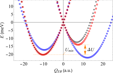
(b)		(c)

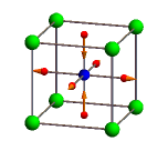
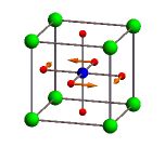
Figure 1: The APES along the $e_{g}\theta$ distortion for Ba₂NaOsO₆ (a), JT distortions for Os (b) and Mo (c) compounds. In (a) the red squares and gray filled circles indicate the APES with and without pseudo JT coupling, respectively, and the blue open circles the APES of linear JT model with pseudo JT coupling. In (b,c), the orange arrows show the direction of the displacements of oxygen atoms at the minima of APES.

Table 2: The position of one of the minima (a.u.) and energy (meV). $\delta l_{\text{max}}$ indicates the largest displacement of oxygen atom under JT deformation, and $U_{\text{min}}$ and $\Delta U$ the JT stabilization energy and the energy barrier between the minima and saddle points, respectively [see Fig. 1].

	Ba2LiOsO6	Ba2NaOsO6	Ba2YMoO6
$Q_{E\theta}$	$-12.29$	$-10.24$	1.42
$Q_{T_{2}\zeta}$	0.00	0.00	11.46
$\delta l_{\text{max}}$	0.022	0.018	0.018
$U_{\text{min}}$	$-32.22$	$-20.31$	$-4.84$
$\Delta U$	10.86	6.27	0.67

IV Jahn-Teller effect

IV.1 Static Jahn-Teller deformation

The derived parameters show that the energy scales for the multiplet splitting and vibrational frequencies $\omega_{\Lambda}$ are comparable, particularly in the case of Ba₂YMoO₆. This makes relevant the pseudo JT effect between $\Gamma_{7}$ and $\Gamma_{8}$ multiplets, along with JT effect in each of them. Indeed, the adiabatic potential energy surfaces (APES) along the JT distortion with and without pseudo JT coupling show non-negligible differences: the APES of $\Gamma_{8}\otimes e_{g}$ JT model (gray circles) is modified (red squares) even in the case of Ba${}_{2}A$OsO₆ with large $\lambda_{\text{SO}}$ [Fig. 1(a)]. Thus, for the adequate description of $d^{1}$ site, the consideration of the full $(\Gamma_{7}\oplus\Gamma_{8})\otimes(e_{g}\oplus t_{2g})$ JT coupling is essential. Fig. 1(a) also shows the unexpectedly strong effect of nonlinear vibronic coupling: the positions of the minima and saddle point of the APES within linear model (blue circles) are inverted by nonlinear coupling (red squares).

The global minima and saddle points of the APES were investigated as in simpler case of $\Gamma_{8}\otimes(e_{g}\oplus t_{2g})$ JT problem Liehr (1963) (for details, see SM ). The results are summarized in Table 2. The static JT distortions for Ba${}_{2}A$OsO₆ develop only along the $e_{g}$ mode [Fig. 1(b)]. The JT stabilization energies $|U_{\text{min}}|$ are 32.2 and 20.3 meV and the energy barriers $\Delta U$ between the minima and the saddle points in the bottom of the APES are only 10.9 and 6.3 meV for $A=$ Li and Na, respectively [see for $A=$ Na Fig. 1(a)]. On the contrary, in Ba₂YMoO₆ the $t_{2g}$ distortion is dominant [Fig. 1(c)]. The stabilization energy is only 4.8 meV Note (2) and the energy barrier at the trigonal point ($Q_{T_{2}\xi}=Q_{T_{2}\eta}=Q_{T_{2}\zeta}$) is about 0.7 meV.

In all materials, the largest shifts $\delta l_{\text{max}}$ of oxygen atom by the static JT deformation were obtained about 0.02 Å which is larger than the experimental resolution , which at a glance seems to be contradictory to the absence of the symmetry lowering in the structural data. However, because of the small warping of the trough $\Delta U$, the dynamical Jahn-Teller effect Bersuker and Polinger (1989); Kaplan and Vekhter (1995), which causes the delocalization of the nuclear wave function over the trough, has to be fully taken into account.

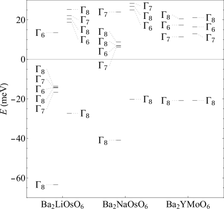
Figure 2: Low-energy vibronic levels in double perovskites (meV). Left and right columns for each compound are the vibronic levels without and with nonlinear vibronic coupling. The ground energy without vibronic coupling is taken as zero of energy.

IV.2 Spin-orbital-lattice entangled states

The vibronic eigenstates of the $(\Gamma_{7}\oplus\Gamma_{8})\otimes(e_{g}\oplus t_{2g})$ JT system have spin-orbital-lattice entangled form:

$$|\Psi_{\alpha\Lambda M}\rangle = \sum_{\Gamma=\Gamma_{7},\Gamma_{8}}\sum_{N}|\Gamma N\rangle\otimes|\psi_{\Gamma N,\alpha\Lambda M}\rangle,$$ (5)

where, $\alpha$ is the principal quantum number, $|\Gamma N\rangle$ is the multiplet state, and $|\psi_{\Gamma N,\alpha\Lambda M}\rangle$ is the nuclear part. The latter is expanded into the eigenstates of harmonic oscillators Kahn and Kettle (1972, 1975); Iwahara et al. (2017). The vibronic states (5) were obtained by numerical diagonalization of the JT Hamiltonian (see Appendix B.4).

Fig. 2 shows the vibronic levels without and with nonlinear vibronic coupling for each system. In Ba${}_{2}A$OsO₆, the nonlinear vibronic coupling significantly destabilizes the linear vibronic states, which is explained by the rise of the minima of APES and reduced magnitude of distortion at the minima [Fig. 1(a)] . The resultant dynamical JT stabilizations are several times larger than the exchange interactions measured by Curie-Weiss constants $\Theta$ ($|\Theta|=$ 3.5 meV for $A=$ Li and 0.9-2.8 meV for $A=$ Na Stitzer et al. (2002); Erickson et al. (2007)). Moreover, a rather weak intersite elastic interaction is expected because OsO₆ octahedrons have no common ligand atoms. The absence of clear static cooperative JT effect (or orbital ordering) Erickson et al. (2007) is explained by its destruction by the unquenched JT dynamics, as is also the case in fullerides Iwahara and Chibotaru (2013). The presence of the JT dynamics means that the phase of the materials should be described in terms of the spin-orbital-lattice entangled states instead of spin or spin-orbit coupled states. Thus, for example, the low-temperature ordered phase Stitzer et al. (2002) is not simple magnetic one but that of spin-orbital-lattice entangled states. The impact of the difference on the physical properties will be discussed in Sec. V.2.

In the case of Ba₂YMoO₆, the energy gain by the JT dynamics amounts to as much as three times the static JT energy (as usual in weak JT regime Bersuker and Polinger (1989)). The dynamical JT stabilization is comparable in magnitude to the reported $\Theta$’s ($|\Theta|$ ranges from 7.8 to 18.9 meV Cussen et al. (2006); Aharen et al. (2010a); de Vries et al. (2010, 2013); Qu et al. (2013). see Table 3), implying non-negligible contribution of the JT dynamics to the low-energy states as discussed above. The first excited states arise at ca 30 meV above the ground one (Fig. 2), which should be put in correspondence to the excitation at ca 28 meV observed in inelastic neutron scattering measurements Carlo et al. (2011). The presence of the JT dynamics does not contradict the temperature evolution of the infrared spectra which was attributed to the classical JT distortion at low temperature Qu et al. (2013). Indeed, a similar temperature dependence of infrared spectra of fullerides was explained on the basis of dynamical JT effect Matsuda et al. .

(a)

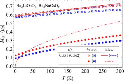
(b)

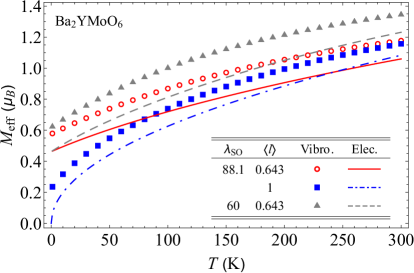
Figure 3: Effective magnetic moments $M_{\text{eff}}$ as function of temperature for (a) Os and (b) Mo compounds. The meaning of the symbols or lines is given in corresponding insets. “Vibro.” and “Elec.” stand for $M_{\text{eff}}$ calculated for dynamical JT states and for pure electronic multiplet states, respectively, and $\langle l\rangle$ (also $\lambda_{\text{SO}}$ for Mo system) is the value used for the simulation. (a) The red circles, solid and dot dashed lines are for Ba₂LiOsO₆, and the blue squares and dashed line are for Ba₂NaOsO₆.

Table 3: Theoretical and experimental effective magnetic moments $M_{\text{eff}}$ ($\mu_{\text{B}}$) and Curie-Weiss temperature $\Theta$ (meV). $T$ (K) indicates the temperature for the simulation or measurements.

	$M_{\text{eff}}$	$\Theta$	$T$	Method	Ref.
— High $T$ —
Ba2LiOsO6	0.707	-	300	Theor. (Vibro.)	Present
	0.733	$-3.5$	150-300	$\chi$	Stitzer et al. (2002)
Ba2NaOsO6	0.658	-	300	Theor. (Vibro.)	Present
	0.677	$-2.8$	150-300	$\chi$	Stitzer et al. (2002)
	0.596-0.647	$-0.9$ - $-1.3$	75-200	$\chi$	Erickson et al. (2007)
Ba2YMoO6	1.351	-	300	Theor. (Vibro.)	Present
	1.231	-	300	Theor. (Elec.)	Present
	1.34	$-7.8$	220-300	$\chi$	Cussen et al. (2006)
	1.41	$-13.8$	150-300	$\chi$	de Vries et al. (2010)
	1.72	$-18.9$	150-300	$\chi$	Aharen et al. (2010a)
	1.44	$-12.3$	160-390	$\chi$	de Vries et al. (2013)
	1.52	$-14.8$	150-300	$\chi$	Qu et al. (2013)
— Low $T$ —
Ba2LiOsO6	0.595	-	0	Theor. (Vibro.)	Present
Ba2NaOsO6	0.569	-	0	Theor. (Vibro.)	Present
	$\approx$ 0.6	-	$\lesssim 10$	NMR	Lu et al. (2017)
Ba2YMoO6	0.624	-	0	Theor. (Vibro.)	Present
	0.462	-	0	Theor. (Elec.)	Present
	0.53	-	$<$ 40	NMR	Aharen et al. (2010a)
	0.59	-	$<$ 25	$\chi$	de Vries et al. (2013)
	0.57	-	$<$ 25	$\chi$	Qu et al. (2013)

V Magnetic properties

In the present systems, the vibronic states (5) inherit the paramagnetic properties from the spin-orbit multiplets. Particularly, because of the entanglement, the lattice degrees of freedom becomes also relevant to the magnetism. Below, two aspects are investigated.

V.1 Effective magnetic moment

The effective magnetic moment $M_{\text{eff}}$ derived from the magnetic susceptibility $\chi$ at high temperature ($T>|\Theta|$) is expected to be close to that of a single $d^{1}$ site because the influence of intersite interactions in this case can be neglected. The temperature dependence of $M_{\text{eff}}$ was calculated with (points) and without (lines) dynamical JT effect (Fig. 3). At $T=0$ K, $M_{\text{eff}}$ arises from the $\Gamma_{8}$ vibronic states only, and as temperature rises it grows due to Van Vleck’s second order contribution Kotani (1949, 1960). The vibronic coupling influences $M_{\text{eff}}$ in two ways: (i) JT coupling to $\Gamma_{8}$ multiplet modifies (often reduces) the matrix element of the electronic operator Child and Longuet-Higgins (1961); Ham (1968); Iwahara et al. (2017) and (ii) pseudo JT coupling mixes the $\Gamma_{7}$ and $\Gamma_{8}$ multiplets. In the present case, the admixture of the $\Gamma_{7}$ multiplet with large magnetic moment leads to the enhancement of $M_{\text{eff}}$.

In the case of Ba${}_{2}A$OsO₆, due to the strong $\hat{H}_{\text{SO}}$, the Van Vleck contribution is small and the temperature dependence of $M_{\text{eff}}$ is weak [Fig. 3(a)]. The theoretical values with DFT $\langle l\rangle$ are in good agreement with the experimental data both at low and high temperature: $M_{\text{eff}}\approx 0.6\mu_{\text{B}}$ at $T\approx 0$ K Lu et al. (2017) and 0.60-0.68$\mu_{\text{B}}$ at high-$T$ Stitzer et al. (2002); Erickson et al. (2007) for Ba₂NaOsO₆ and 0.73$\mu_{\text{B}}$ at high-$T$ for Ba₂LiOsO₆ Stitzer et al. (2002). As widely accepted Aharen et al. (2010a); Gangopadhyay and Pickett (2015); Xu et al. (2016); Ahn et al. (2017), the $d$-$p$ hybridization of Os and O atoms enlarges electronic $M_{\text{eff}}$ (compare the data for the DFT-derived $\langle l\rangle$ and the atomic value). The JT dynamics slightly quenches the variation of $M_{\text{eff}}$ [Fig. 3(a)].

On the other hand, in Ba₂YMoO₆, the pseudo JT coupling plays a crucial role to enhance $M_{\text{eff}}$ [Fig. 3(b)]. At $T=0$ K, $M_{\text{eff}}$ amounts to 0.6$\mu_{\text{B}}$, which is in line with NMR 0.53$\mu_{\text{B}}$ Aharen et al. (2010a) and low-$T$ susceptibility 0.57-0.59$\mu_{\text{B}}$ de Vries et al. (2013); Qu et al. (2013), and it rapidly grows with $T$. Taking into account the covalency effect on both $\lambda_{\text{SO}}$ and $\langle l\rangle$ (gray triangles), $M_{\text{eff}}$ at $T\approx 300$ K reaches the experimental values (1.3-1.5$\mu_{\text{B}}$ Cussen et al. (2006); de Vries et al. (2010, 2013); Qu et al. (2013)).

(a)	(b)
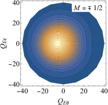
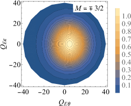
(c)

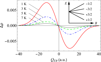
Figure 4: (a), (b) $\rho_{\Gamma_{8}M}(Q_{\theta},Q_{\epsilon})$ for $M=\mp\frac{1}{2}$ and $\mp\frac{3}{2}$, respectively, and (c) the temperature evolution of the distribution of vibronic states for Ba₂NaOsO₆. In (a), (b), the contour lines are drawn from 0 with increment of 1/20. In (c), the distribution with respect to averaged one $\Delta\rho$ is shown under applied field of $|\bm{B}|=15$ T. The inset shows the Zeeman splitting of the $\Gamma_{8}$ vibronic state. For the description of $\Delta\rho$, see Appendix B.6.

V.2 Spin-orbital-lattice entanglement driven magneto-elastic response

A peculiarity of the present systems is that the Zeeman splitting is accompanied by the variation of the $Q_{\Lambda\lambda}$ distribution in the ground $\Gamma_{8}$ vibronic state,

$$\rho_{\Gamma_{8}M}(\bm{Q})=\langle\Psi_{\Gamma_{8}M}|\bm{Q}\rangle\langle\bm{Q}|\Psi_{\Gamma_{8}M}\rangle,$$ (6)

where, $\bm{Q}$ is a set of normal coordinates. Under $\bm{B}\parallel[001]$ the ground $\Gamma_{8}$ level split as in the inset of Fig. 4(c). In the case of Os compounds, slight localization at the minima in the APES is observed for $|\Psi_{\Gamma_{8},\mp\frac{1}{2}}\rangle$, and around the saddle point for $|\Psi_{\Gamma_{8},\mp\frac{3}{2}}\rangle$ [see for the case of Ba₂NaOsO₆ Fig. 4(a), (b)]. Thus, with the increase of temperature, the center of the distribution $\rho$ shifts from the minima of APES to the symmetric point [Fig. 1(c). See for the definition of $\rho$ Appendix B.6].

The temperature evolution of $\rho$ must be related to the observation of the “broken local point symmetry” in Ba₂NaOsO₆ Lu et al. (2017); Liu et al. (2018). The expectation value of the JT distortion is reduced by the JT dynamics, and it is consistent with the expected small JT deformation in the NMR study as well as x-ray data Erickson et al. (2007). Besides the applied field, the exchange interaction between $d^{1}$ centers enhances the Zeeman splitting in the presence of magnetic order, which would cause the reduction of the magnetic entropy to $k_{\text{B}}\ln 2$ Erickson et al. (2007). Thus, the ordering in Ba₂NaOsO₆ Lu et al. (2017) is not a conventional orbital ordering with classical (static) JT distortions but an ordering of spin-orbital-lattice entangled states.

Contrary to the Os compounds, in Ba₂YMoO₆ no magnetic order develops down to 50 mK de Vries et al. (2013). Despite the stronger exchange interaction Cussen et al. (2006); Aharen et al. (2010a); de Vries et al. (2010, 2013); Qu et al. (2013) than in Ba${}_{2}A$OsO₆, the absence of the ordering hinders the large Zeeman splitting of vibronic levels, and hence, the dynamical JT effect develops as supported by neutron diffraction data Aharen et al. (2010a) and sustains the magnetic entropy of $k_{\text{B}}\ln 4$ observed by muon spin resonance de Vries et al. (2010).

VI Conclusion

The local spin-orbital-lattice entangled states of three cubic $d^{1}$ double perovskites were derived based on the first principle approach. The gain of the energy of the ground coupled states is larger than (Ba${}_{2}A$OsO₆) or comparable to (Ba₂YMoO₆) the corresponding Curie-Weiss constants, suggesting the presence of dynamical JT effect in these materials. Due to the mixing with spin degrees of freedom, the vibronic states respond strongly to the magnetic field. Thus, the first excited vibronic level at $\approx 30$ meV in Ba₂YMoO₆ suggests its relevance to the magnetic excitations measured in inelastic neutron scattering. In this compound, the vibronic coupling involving both $\Gamma_{8}$ and $\Gamma_{7}$ multiplets gives rise to strong temperature dependence of the effective magnetic moment. In Ba${}_{2}A$OsO₆, the entanglement gives rise to magneto-elastic response where a small static component of the dynamical JT deformation accompanies the Zeeman splitting, which explains the “breaking of local point symmetry”.

The relevance of the spin-orbital-lattice entanglement is expected in other cubic $d^{1}$ Cussen et al. (2006); Coomer and Cussen (2013); Marjerrison et al. (2016a) and $d^{2}$ double perovskites Yamamura et al. (2006); Aharen et al. (2010b); Thompson et al. (2014); Marjerrison et al. (2016b); Feng et al. (2016), and also in other types of cubic crystals such as $5d^{1}$ Ta chlorides persisting cubic symmetry down to low temperature Ishikawa et al. . For the complete understanding of the unconventional magnetic phases of the family of cubic double perovskites containing heavy transition metal, concomitant treatment of the vibronic and magnetic interactions is found to be crucial. The ordering of the spin-orbital-lattice entangled states would be a new direction towards unconventional multifunctional materials.

Appendix A Derivation of the model Hamiltonian

Here, the transformation of the model Hamiltonian for $t_{2g}^{1}$ ion in an octahedral environment into the one in the basis of spin-orbit coupled states is shown in detail. In this section, the operators for the spin-orbital decoupled and coupled states by lower and upper cases, respectively, the subscript $g$ of the representations is omitted in the equations for simplicity, and the coordinate axes of the $d^{1}$ system are chosen to correspond to $C_{4}$ axes.

According to the selection rule for the $t_{2g}$ orbitals,

$$t_{2g}\otimes t_{2g}=a_{1g}\oplus e_{g}\oplus\{t_{1g}\}\oplus t_{2g},$$ (7)

the $t_{2g}$ orbitals have unquenched orbital angular momenta (time-odd $t_{1g}$ operator) and also couple to the $a_{1g}$, $e_{g}$ and $t_{2g}$ vibrational modes (Fig. 5). In Eq. (7), the curly bracket indicates that the representation is antisymmetric.

(a) $e_{g}\theta$	(b) $e_{g}\epsilon$	(c) $t_{2g}\zeta$

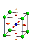
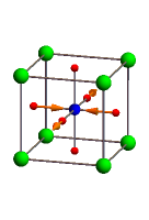
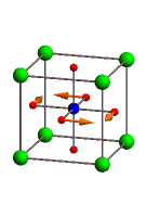
Figure 5: Symmetrized mass-weighted normal vibrations. (a) $E_{g}\theta$, (b) $E_{g}\epsilon$, (c) $T_{2g}\zeta$.

A.1 Electronic states

The presence of the unquenched orbital angular momenta indicates the spin-orbit coupling acts on $t_{2g}^{1}$ configurations in the first order of perturbation. Projecting the orbital angular momentum operator for the $d$ orbitals into the space of $t_{2g}$ orbitals, we obtain

$$\hat{\bm{l}} = \langle l\rangle\tilde{\bm{l}},$$ (8)

where, the reduction of the orbital angular momentum by the covalency effect is included in $\langle l\rangle$, the components of $\tilde{\bm{l}}$ are written as follows Kotani (1960); Sugano et al. (1970):

$$\tilde{l}_{x} = \begin{pmatrix}0&0&0\\ 0&0&i\\ 0&-i&0\end{pmatrix},\quad\tilde{l}_{y}=\begin{pmatrix}0&0&-i\\ 0&0&0\\ i&0&0\end{pmatrix},$$

$$\quad\tilde{l}_{z} = \begin{pmatrix}0&i&0\\ -i&0&0\\ 0&0&0\end{pmatrix},$$ (9)

in the order of the electronic basis $|t_{2}\xi\rangle$, $|t_{2}\eta\rangle$, $|t_{2}\zeta\rangle$. $\xi,\eta,\zeta$ indicate the basis of $t_{2g}$ representation which transform as $yz$, $zx$, $xy$, respectively, under symmetry operation of $O_{h}$ group.

Due to the spin-orbit coupling, $\hat{h}_{\text{SO}}=\lambda_{\text{SO}}\tilde{\bm{l}}\cdot\hat{\bm{s}}$, $t_{2g}^{1}$ configurations split into spin-orbit multiplets Koster et al. (1963):

$$t_{2}\otimes\Gamma_{6}=\Gamma_{7}\oplus\Gamma_{8}.$$ (10)

$\Gamma_{6}$ is the irreducible representation of electron spin state. Since each representation appears only once in the right hand side, the spin-orbit coupled states are determined by using Clebsch-Gordan coefficients as Koster et al. (1963)

$$\left|\Gamma_{7},-\frac{1}{2}\right\rangle = -\frac{i}{\sqrt{3}}|t_{2}\xi,\uparrow\rangle-\frac{1}{\sqrt{3}}|t_{2}\eta,\uparrow\rangle+\frac{i}{\sqrt{3}}|t_{2}\zeta,\downarrow\rangle,$$

$$\left|\Gamma_{7},+\frac{1}{2}\right\rangle = -\frac{i}{\sqrt{3}}|t_{2}\xi,\downarrow\rangle+\frac{1}{\sqrt{3}}|t_{2}\eta,\downarrow\rangle-\frac{i}{\sqrt{3}}|t_{2}\zeta,\uparrow\rangle,$$

$$\left|\Gamma_{8},-\frac{3}{2}\right\rangle = -\frac{i}{\sqrt{6}}|t_{2}\xi,\downarrow\rangle+\frac{1}{\sqrt{6}}|t_{2}\eta,\downarrow\rangle+i\sqrt{\frac{2}{3}}|t_{2}\zeta,\uparrow\rangle,$$

$$\left|\Gamma_{8},-\frac{1}{2}\right\rangle = \frac{i}{\sqrt{2}}|t_{2}\xi,\uparrow\rangle-\frac{1}{\sqrt{2}}|t_{2}\eta,\uparrow\rangle,$$

$$\left|\Gamma_{8},+\frac{1}{2}\right\rangle = -\frac{i}{\sqrt{2}}|t_{2}\xi,\downarrow\rangle-\frac{1}{\sqrt{2}}|t_{2}\eta,\downarrow\rangle,$$

$$\left|\Gamma_{8},+\frac{3}{2}\right\rangle = \frac{i}{\sqrt{6}}|t_{2}\xi,\uparrow\rangle+\frac{1}{\sqrt{6}}|t_{2}\eta,\uparrow\rangle+i\sqrt{\frac{2}{3}}|t_{2}\zeta,\downarrow\rangle.$$

With the use of the spin-orbit coupled basis, Eq. (LABEL:Eq:Gamma78), the magnetic moment (3) in Zeeman Hamiltonian, the matrix forms of the pseudo orbital and spin angular momentum operators are given as

$$\hat{L}_{x} = \begin{pmatrix}0&-\frac{2}{3}&\frac{1}{3\sqrt{2}}&0&\frac{1}{\sqrt{6}}&0\\ -\frac{2}{3}&0&0&-\frac{1}{\sqrt{6}}&0&-\frac{1}{3\sqrt{2}}\\ \frac{1}{3\sqrt{2}}&0&0&\frac{1}{\sqrt{3}}&0&-\frac{2}{3}\\ 0&-\frac{1}{\sqrt{6}}&\frac{1}{\sqrt{3}}&0&0&0\\ \frac{1}{\sqrt{6}}&0&0&0&0&\frac{1}{\sqrt{3}}\\ 0&-\frac{1}{3\sqrt{2}}&-\frac{2}{3}&0&\frac{1}{\sqrt{3}}&0\\ \end{pmatrix},$$

$$\hat{L}_{y} = \begin{pmatrix}0&-\frac{2i}{3}&\frac{i}{3\sqrt{2}}&0&-\frac{i}{\sqrt{6}}&0\\ \frac{2i}{3}&0&0&-\frac{i}{\sqrt{6}}&0&\frac{i}{3\sqrt{2}}\\ -\frac{i}{3\sqrt{2}}&0&0&\frac{i}{\sqrt{3}}&0&\frac{2i}{3}\\ 0&\frac{i}{\sqrt{6}}&-\frac{i}{\sqrt{3}}&0&0&0\\ \frac{i}{\sqrt{6}}&0&0&0&0&\frac{i}{\sqrt{3}}\\ 0&-\frac{i}{3\sqrt{2}}&-\frac{2i}{3}&0&-\frac{i}{\sqrt{3}}&0\\ \end{pmatrix},$$

$$\hat{L}_{z} = \begin{pmatrix}\frac{2}{3}&0&0&0&0&-\frac{\sqrt{2}}{3}\\ 0&-\frac{2}{3}&-\frac{\sqrt{2}}{3}&0&0&0\\ 0&-\frac{\sqrt{2}}{3}&-\frac{1}{3}&0&0&0\\ 0&0&0&-1&0&0\\ 0&0&0&0&1&0\\ -\frac{\sqrt{2}}{3}&0&0&0&0&\frac{1}{3}\end{pmatrix},$$ (12)

and

$$\hat{S}_{x} = \begin{pmatrix}0&-\frac{1}{6}&\frac{1}{3\sqrt{2}}&0&\frac{1}{\sqrt{6}}&0\\ -\frac{1}{6}&0&0&-\frac{1}{\sqrt{6}}&0&-\frac{1}{3\sqrt{2}}\\ \frac{1}{3\sqrt{2}}&0&0&-\frac{1}{2\sqrt{3}}&0&\frac{1}{3}\\ 0&-\frac{1}{\sqrt{6}}&-\frac{1}{2\sqrt{3}}&0&0&0\\ \frac{1}{\sqrt{6}}&0&0&0&0&-\frac{1}{2\sqrt{3}}\\ 0&-\frac{1}{3\sqrt{2}}&\frac{1}{3}&0&-\frac{1}{2\sqrt{3}}&0\\ \end{pmatrix},$$

$$\hat{S}_{y} = \begin{pmatrix}0&-\frac{i}{6}&\frac{i}{3\sqrt{2}}&0&-\frac{i}{\sqrt{6}}&0\\ \frac{i}{6}&0&0&-\frac{i}{\sqrt{6}}&0&\frac{i}{3\sqrt{2}}\\ -\frac{i}{3\sqrt{2}}&0&0&-\frac{i}{2\sqrt{3}}&0&-\frac{i}{3}\\ 0&\frac{i}{\sqrt{6}}&\frac{i}{2\sqrt{3}}&0&0&0\\ \frac{i}{\sqrt{6}}&0&0&0&0&-\frac{i}{2\sqrt{3}}\\ 0&-\frac{i}{3\sqrt{2}}&\frac{i}{3}&0&\frac{i}{2\sqrt{3}}&0\\ \end{pmatrix},$$

$$\hat{S}_{z} = \begin{pmatrix}\frac{1}{6}&0&0&0&0&-\frac{\sqrt{2}}{3}\\ 0&-\frac{1}{6}&-\frac{\sqrt{2}}{3}&0&0&0\\ 0&-\frac{\sqrt{2}}{3}&\frac{1}{6}&0&0&0\\ 0&0&0&\frac{1}{2}&0&0\\ 0&0&0&0&-\frac{1}{2}&0\\ -\frac{\sqrt{2}}{3}&0&0&0&0&-\frac{1}{6}\end{pmatrix},$$ (13)

respectively. The basis is in the same order as Eq. (LABEL:Eq:Gamma78). The spin-orbit, $\hat{h}_{\text{SO}}=\lambda_{\text{SO}}\tilde{\bm{l}}\cdot\hat{\bm{s}}$, and Zeeman, $\hat{h}_{\text{Zee}}=-\hat{\bm{m}}\cdot\bm{B}$, Hamiltonian matrices in the coupled basis are obtained by simply replacing the $\tilde{\bm{l}}$ and $\hat{\bm{s}}$ by $\hat{\bm{L}}$ and $\hat{\bm{S}}$, respectively.

A.2 Vibronic coupling

The $t_{2g}$ orbital couples to $a_{1g}$, $e_{g}$ and $t_{2g}$ vibrations (7). We take the $O_{h}$ structure which is fully relaxed with respect to the $a_{g}$ normal mode as reference structure. The totally symmetric part contains harmonic and anharmonic potentials:

$$\hat{h}_{A_{1}} = \sum_{\gamma=\theta,\epsilon}\frac{\omega_{E}^{2}}{2}\hat{Q}_{E\gamma}^{2}+\sum_{\gamma=\xi,\eta,\zeta}\frac{\omega_{T_{2}}^{2}}{2}\hat{Q}_{T_{2}\gamma}^{2}$$ (14)

$$+ \sum_{\gamma=\theta,\epsilon}\frac{v_{A_{1}}^{EEE}}{3!}\{\hat{Q}_{E}\otimes\hat{Q}_{E}\otimes\hat{Q}_{E}\}_{A_{1}}$$

$$+ \sum_{\gamma=\theta,\epsilon}\frac{v_{A_{1}}^{EEEE}}{4!}\{\hat{Q}_{E}\otimes\hat{Q}_{E}\otimes\hat{Q}_{E}\otimes\hat{Q}_{E}\}_{A_{1}}.$$

Here, $\omega_{\Gamma}$ is the frequency for $\Gamma$ mode ($\Gamma=E,T_{2}$). The symmetrized products are shown below. The basis of $e_{g}$ representation expressed by $\theta$ and $\epsilon$ transform as $(-x^{2}-y^{2}+2z^{2})/\sqrt{6}$ and $(x^{2}-y^{2})/\sqrt{2}$, respectively, under symmetry operations.

The vibronic couplings with the $e_{g}$ and $t_{2g}$ modes induce the Jahn-Teller effect. The linear term is given by

$$\hat{h}_{\text{LJT}} = \sum_{\gamma=\theta,\epsilon}v_{E}\hat{Q}_{E\gamma}\hat{\tau}_{E\gamma}+\sum_{\gamma=\xi,\eta,\zeta}v_{T_{2}}\hat{Q}_{T_{2}\gamma}\hat{\tau}_{T_{2}\gamma}.$$ (15)

Here, $v_{\Gamma}$ are the linear orbital vibronic coupling parameters, and $\hat{\bm{\tau}}$ are matrices of Clebsch-Gordan coefficients:

$$\hat{\tau}_{E\theta} = \begin{pmatrix}-\frac{1}{2}&0&0\\ 0&-\frac{1}{2}&0\\ 0&0&1\end{pmatrix},\quad\hat{\tau}_{E\epsilon}=\begin{pmatrix}\frac{\sqrt{3}}{2}&0&0\\ 0&-\frac{\sqrt{3}}{2}&0\\ 0&0&0\end{pmatrix},$$

$$\hat{\tau}_{T_{2}\xi} = \begin{pmatrix}0&0&0\\ 0&0&\frac{1}{\sqrt{2}}\\ 0&\frac{1}{\sqrt{2}}&0\\ \end{pmatrix},\quad\hat{\tau}_{T_{2}\eta}=\begin{pmatrix}0&0&\frac{1}{\sqrt{2}}\\ 0&0&0\\ \frac{1}{\sqrt{2}}&0&0\\ \end{pmatrix},$$

$$\hat{\tau}_{T_{2}\zeta} = \begin{pmatrix}0&\frac{1}{\sqrt{2}}&0\\ \frac{1}{\sqrt{2}}&0&0\\ 0&0&0\\ \end{pmatrix}.$$ (16)

The phase factors of the the Jahn-Teller active modes are chosen as shown in Fig. 5.

Transforming the electronic basis from the spin-orbital decoupled states into the coupled states (LABEL:Eq:Gamma78), $\hat{\bm{\tau}}$’s in $\hat{h}_{\text{LJT}}$ become

$$\hat{T}_{E\theta} = \begin{pmatrix}0&0&0&0&0&\frac{1}{\sqrt{2}}\\ 0&0&-\frac{1}{\sqrt{2}}&0&0&0\\ 0&-\frac{1}{\sqrt{2}}&\frac{1}{2}&0&0&0\\ 0&0&0&-\frac{1}{2}&0&0\\ 0&0&0&0&-\frac{1}{2}&0\\ \frac{1}{\sqrt{2}}&0&0&0&0&\frac{1}{2}\end{pmatrix},$$

$$\hat{T}_{E\epsilon} = \begin{pmatrix}0&0&0&-\frac{1}{\sqrt{2}}&0&0\\ 0&0&0&0&\frac{1}{\sqrt{2}}&0\\ 0&0&0&0&\frac{1}{2}&0\\ -\frac{1}{\sqrt{2}}&0&0&0&0&\frac{1}{2}\\ 0&\frac{1}{\sqrt{2}}&\frac{1}{2}&0&0&0\\ 0&0&0&\frac{1}{2}&0&0\\ \end{pmatrix},$$

$$\hat{T}_{T_{2}\xi} = \begin{pmatrix}0&0&-\frac{i}{2}&0&\frac{i}{2\sqrt{3}}&0\\ 0&0&0&-\frac{i}{2\sqrt{3}}&0&\frac{i}{2}\\ \frac{i}{2}&0&0&\frac{i}{\sqrt{6}}&0&0\\ 0&\frac{i}{2\sqrt{3}}&-\frac{i}{\sqrt{6}}&0&0&0\\ -\frac{i}{2\sqrt{3}}&0&0&0&0&-\frac{i}{\sqrt{6}}\\ 0&-\frac{i}{2}&0&0&\frac{i}{\sqrt{6}}&0\\ \end{pmatrix},$$

$$\hat{T}_{T_{2}\eta} = \begin{pmatrix}0&0&-\frac{1}{2}&0&-\frac{1}{2\sqrt{3}}&0\\ 0&0&0&-\frac{1}{2\sqrt{3}}&0&-\frac{1}{2}\\ -\frac{1}{2}&0&0&\frac{1}{\sqrt{6}}&0&0\\ 0&-\frac{1}{2\sqrt{3}}&\frac{1}{\sqrt{6}}&0&0&0\\ -\frac{1}{2\sqrt{3}}&0&0&0&0&-\frac{1}{\sqrt{6}}\\ 0&-\frac{1}{2}&0&0&-\frac{1}{\sqrt{6}}&0\\ \end{pmatrix},$$

$$\hat{T}_{T_{2}\zeta} = \begin{pmatrix}0&0&0&-\frac{i}{\sqrt{3}}&0&0\\ 0&0&0&0&-\frac{i}{\sqrt{3}}&0\\ 0&0&0&0&-\frac{i}{\sqrt{6}}&0\\ \frac{i}{\sqrt{3}}&0&0&0&0&-\frac{i}{\sqrt{6}}\\ 0&\frac{i}{\sqrt{3}}&\frac{i}{\sqrt{6}}&0&0&0\\ 0&0&0&\frac{i}{\sqrt{6}}&0&0\\ \end{pmatrix}.$$ (17)

Replacing $\hat{\bm{\tau}}$ in $\hat{h}_{\text{LJT}}$ with $\hat{\bm{T}}$, we obtain $\hat{H}_{\text{LJT}}$.

The non-linear vibronic Hamiltonian is derived in the same manner:

$$\hat{h}_{\text{NLJT}} = \sum_{\gamma=\theta,\epsilon}\frac{v_{E}^{EE}}{2!}\{\hat{Q}_{E}\otimes\hat{Q}_{E}\}_{E\gamma}\hat{\tau}_{E\gamma}$$

$$+ \sum_{\gamma=\theta,\epsilon}\frac{v_{E}^{T_{2}T_{2}}}{2!}\{\hat{Q}_{T_{2}}\otimes\hat{Q}_{T_{2}}\}_{E\gamma}\hat{\tau}_{E\gamma}$$

$$+ \sum_{\gamma=\xi,\eta,\zeta}\frac{v_{T_{2}}^{T_{2}T_{2}}}{2!}\{\hat{Q}_{T_{2}}\otimes\hat{Q}_{T_{2}}\}_{T_{2}\gamma}\hat{\tau}_{T_{2}\gamma}$$

$$+ \sum_{\gamma=\xi,\eta,\zeta}\frac{v_{T_{2}}^{ET_{2}}}{2!}\{\hat{Q}_{E}\otimes\hat{Q}_{T_{2}}\}_{T_{2}\gamma}\hat{\tau}_{T_{2}\gamma}$$

$$+ \sum_{\gamma=\theta,\epsilon}\frac{v_{E}^{EEE}}{3!}\{\hat{Q}_{E}\otimes\hat{Q}_{E}\otimes\hat{Q}_{E}\}_{E\gamma}\hat{\tau}_{E\gamma}$$

$$+ \sum_{n=1,2}\sum_{\gamma=\theta,\epsilon}\frac{v_{nE}^{EEEE}}{4!}\{\hat{Q}_{E}\otimes\hat{Q}_{E}\otimes\hat{Q}_{E}\otimes\hat{Q}_{E}\}_{nE\gamma}\hat{\tau}_{E\gamma}.$$

Here, only the terms treated in this work are written. By the same transformation as $\hat{h}_{\text{LJT}}$, we obtain $\hat{H}_{\text{NLJT}}$.

The symmetrized products of the coordinates appearing in Eqs. (14) and (LABEL:Eq:hNLJT) are calculated as follows. The symmetrized quadratic coordinates are in general calculated as

$$\{\hat{Q}_{\Lambda_{1}}\otimes\hat{Q}_{\Lambda_{2}}\}_{\Lambda\lambda} = \sum_{\lambda_{1}\lambda_{2}}\hat{Q}_{\Lambda_{1}\lambda_{1}}\hat{Q}_{\Lambda_{2}\lambda_{2}}$$ (19)

$$\times \langle\Lambda_{1}\lambda_{1}\Lambda_{2}\lambda_{2}|(\Lambda_{1}\Lambda_{2})\Lambda\lambda\rangle.$$

Here, $\langle\Lambda_{1}\lambda_{1}\Lambda_{2}\lambda_{2}|(\Lambda_{1}\Lambda_{2})\Lambda\lambda\rangle$ is Clebsch-Gordan coefficient tabulated in Ref. Koster et al. (1963). The explicit form of the symmetrized products of our interests are

$$\{\hat{Q}_{E}\otimes\hat{Q}_{E}\}_{A} = \frac{1}{\sqrt{2}}\left(\hat{Q}_{E\theta}^{2}+\hat{Q}_{E\epsilon}^{2}\right),$$

$$\{\hat{Q}_{T_{2}}\otimes\hat{Q}_{T_{2}}\}_{A} = \frac{1}{\sqrt{3}}\left(\hat{Q}_{T_{2}\xi}^{2}+\hat{Q}_{T_{2}\eta}^{2}+\hat{Q}_{T_{2}\zeta}^{2}\right),$$

$$\{\hat{Q}_{E}\otimes\hat{Q}_{E}\}_{E\theta} = -\frac{1}{\sqrt{2}}\left(\hat{Q}_{E\theta}^{2}-\hat{Q}_{E\epsilon}^{2}\right),$$

$$\{\hat{Q}_{E}\otimes\hat{Q}_{E}\}_{E\epsilon} = \sqrt{2}\hat{Q}_{E\theta}\hat{Q}_{E\epsilon},$$

$$\{\hat{Q}_{T_{2}}\otimes\hat{Q}_{T_{2}}\}_{E\theta} = -\frac{1}{\sqrt{6}}\left(\hat{Q}_{T_{2}\xi}^{2}+\hat{Q}_{T_{2}\eta}^{2}-2\hat{Q}_{T_{2}\zeta}^{2}\right),$$

$$\{\hat{Q}_{T_{2}}\otimes\hat{Q}_{T_{2}}\}_{E\epsilon} = \frac{1}{\sqrt{2}}\left(\hat{Q}_{T_{2}\xi}^{2}-\hat{Q}_{T_{2}\eta}^{2}\right),$$

$$\{\hat{Q}_{T_{2}}\otimes\hat{Q}_{T_{2}}\}_{T_{2}\xi} = \sqrt{2}\hat{Q}_{T_{2}\eta}\hat{Q}_{T_{2}\zeta},$$

$$\{\hat{Q}_{T_{2}}\otimes\hat{Q}_{T_{2}}\}_{T_{2}\eta} = \sqrt{2}\hat{Q}_{T_{2}\zeta}\hat{Q}_{T_{2}\xi},$$

$$\{\hat{Q}_{T_{2}}\otimes\hat{Q}_{T_{2}}\}_{T_{2}\zeta} = \sqrt{2}\hat{Q}_{T_{2}\xi}\hat{Q}_{T_{2}\eta},$$

$$\{\hat{Q}_{E}\otimes\hat{Q}_{T_{2}}\}_{T_{2}\xi} = \left(-\frac{1}{2}\hat{Q}_{E\theta}+\frac{\sqrt{3}}{2}\hat{Q}_{E\epsilon}\right)\hat{Q}_{T_{2}\xi},$$

$$\{\hat{Q}_{E}\otimes\hat{Q}_{T_{2}}\}_{T_{2}\eta} = \left(-\frac{1}{2}\hat{Q}_{E\theta}-\frac{\sqrt{3}}{2}\hat{Q}_{E\epsilon}\right)\hat{Q}_{T_{2}\eta},$$

$$\{\hat{Q}_{E}\otimes\hat{Q}_{T_{2}}\}_{T_{2}\zeta} = \hat{Q}_{E\theta}\hat{Q}_{T_{2}\zeta},$$ (20)

for quadratic terms. The cubic products can be calculated by using Eq. (19) twice. The cubic terms of our interest are calculated as follows:

$$\{\hat{Q}_{E}\otimes\{\hat{Q}_{E}\otimes\hat{Q}_{E}\}_{E}\}_{A_{1}} = \frac{1}{2}\left(-\hat{Q}_{E\theta}^{3}+3\hat{Q}_{E\theta}\hat{Q}_{E\epsilon}^{2}\right),$$

$$\{\hat{Q}_{E}\otimes\{\hat{Q}_{E}\otimes\hat{Q}_{E}\}_{E}\}_{E\theta} = \frac{1}{2}\hat{Q}_{E\theta}\left(\hat{Q}_{E\theta}^{2}+\hat{Q}_{E\epsilon}^{2}\right),$$

$$\{\hat{Q}_{E}\otimes\{\hat{Q}_{E}\otimes\hat{Q}_{E}\}_{E}\}_{E\theta} = \frac{1}{2}\hat{Q}_{E\epsilon}\left(\hat{Q}_{E\theta}^{2}+\hat{Q}_{E\epsilon}^{2}\right).$$ (21)

The fourth order terms for the $E$ mode are calculated as

$$\{\hat{Q}_{E}\otimes\hat{Q}_{E}\otimes\hat{Q}_{E}\otimes\hat{Q}_{E}\}_{A_{1}} = \{\hat{Q}_{E}\otimes\hat{Q}_{E}\}_{A_{1}}^{2}=\frac{1}{2}\left(\hat{Q}_{E\theta}^{2}+\hat{Q}_{E\epsilon}^{2}\right)^{2},$$

$$\{\hat{Q}_{E}\otimes\hat{Q}_{E}\otimes\hat{Q}_{E}\otimes\hat{Q}_{E}\}_{1E\theta} = \{\hat{Q}_{E}\otimes\hat{Q}_{E}\}_{A_{1}}\{\hat{Q}_{E}\otimes\hat{Q}_{E}\}_{E\theta}=-\frac{1}{2}\left(\hat{Q}_{E\theta}^{2}-\hat{Q}_{E\epsilon}^{2}\right)\left(\hat{Q}_{E\theta}^{2}+\hat{Q}_{E\epsilon}^{2}\right),$$

$$\{\hat{Q}_{E}\otimes\hat{Q}_{E}\otimes\hat{Q}_{E}\otimes\hat{Q}_{E}\}_{1E\epsilon} = \{\hat{Q}_{E}\otimes\hat{Q}_{E}\}_{A_{1}}\{\hat{Q}_{E}\otimes\hat{Q}_{E}\}_{E\epsilon}=\hat{Q}_{E\theta}\hat{Q}_{E\epsilon}\left(\hat{Q}_{E\theta}^{2}+\hat{Q}_{E\epsilon}^{2}\right),$$

$$\{\hat{Q}_{E}\otimes\hat{Q}_{E}\otimes\hat{Q}_{E}\otimes\hat{Q}_{E}\}_{2E\theta} = \{\{\hat{Q}_{E}\otimes\hat{Q}_{E}\}_{E}\otimes\{\hat{Q}_{E}\otimes\hat{Q}_{E}\}_{E}\}_{E\theta}=-\frac{1}{2\sqrt{2}}\left(\hat{Q}_{E\theta}^{4}+\hat{Q}_{E\epsilon}^{4}-6\hat{Q}_{E\theta}^{2}\hat{Q}_{E\epsilon}^{2}\right),$$

$$\{\hat{Q}_{E}\otimes\hat{Q}_{E}\otimes\hat{Q}_{E}\otimes\hat{Q}_{E}\}_{2E\epsilon} = \{\{\hat{Q}_{E}\otimes\hat{Q}_{E}\}_{E}\otimes\{\hat{Q}_{E}\otimes\hat{Q}_{E}\}_{E}\}_{E\epsilon}=-\sqrt{2}\left(\hat{Q}_{E\theta}^{2}-\hat{Q}_{E\epsilon}^{2}\right)\hat{Q}_{E\theta}\hat{Q}_{E\epsilon}.$$ (22)

Appendix B Computational details

B.1 Ab initio Method

The electronic and vibronic coupling parameters were derived from the cluster calculations with post Hartree-Fock (HF) methods and $\langle l\rangle$’s were extracted with density functional theory (DFT) calculations. The clusters were generated from the experimental crystal structures Aharen et al. (2010a); Stitzer et al. (2002) retaining the $O_{h}$ symmetry. In the post HF calculations, the $d^{1}$ metal ion and the nearest six oxygen atoms were treated ab initio with ANO-RCC-VQZP basis functions and the surrounding 280 atoms were replaced by ab initio embedding model potential (AIMP) Seijo and Barandiarán (1999). The atomic bielectronic integrals were calculated using Cholesky decomposition with threshold $1\times 10^{-9}$ $E_{h}$. Inversion symmetry was employed in all calculations.

All ab initio calculations were carried out with Molcas 8.0 program Aquilante et al. (2016) and were of complete-active-space self-consistent-field (CASSCF)/extended multi-state complete active space second-order perturbation theory (XMS-CASPT2) Granovsky (2011); Shiozaki et al. (2011)/spin-orbit restricted-active-space state-interaction (SO-RASSI) type. The active space of all CASSCF calculations included seven electrons in six orbitals. Three orbitals are $4d$ or $5d$ orbitals and other three orbitals are of ligand $\pi$-type. Three roots were optimized at the CASSCF level, and then XMS-CASPT2 were done on the 3 roots from CASSCF. In XMS-CASPT2 calculations, IPEA shift was set to 0, while IMAG shift was set to 0.1. SO-RASSI calculations mixed the roots obtained from XMS-CASPT2 by spin-orbit coupling. The scalar relativistic effects were included in the basis set.

B.2 DFT Method

The clusters for the DFT calculations contain 89 atoms which are treated explicitly with def2-TZVP basis set and def2/J auxiliary basis sets. DFT calculations were done with hybrid functional B3LYP with RIJCOSX approximation. The basis function contains the scalar relativistic effects. For the DFT calculations, ORCA 4.0.0.2 Neese (2012) was used. For the SCF, condition “TightSCF” is used. The grid for density was “Grid5”.

B.3 Calculations of electronic and vibronic coupling parameters

The spin-orbit coupling parameters $\lambda_{\text{SO}}$ were obtained from the ab initio multiplet levels, $E_{\Gamma_{7}}-E_{\Gamma_{8}}=\frac{3}{2}\lambda_{\text{SO}}$. The expectation values of orbital angular momentum $\langle l\rangle$ were calculated by using ab initio or DFT wave functions at $O_{h}$ structure. In the latter case, the orbital angular momentum matrices in the atomic orbital basis were calculated using Molpro 2012.1 Werner et al. (2012).

The frequencies and vibronic parameters were derived by fitting the ab initio ${}^{2}T_{2g}$ adiabatic potential energy surface (APES) to the $t_{2g}\otimes(e_{g}\oplus t_{2g})$ model vibronic Hamiltonian SM . The step of deformation is $\Delta Q=0.5$ a.u. The unit of $k$-th order vibronic coupling parameter is $E_{h}/(m_{e}a_{0}^{2})^{k/2}$, where, $E_{h}$ is Hartree, $m_{e}$ is electron mass and $a_{0}$ is Bohr radius.

B.4 Numerical diagonalization of vibronic Hamiltonian

The $(\Gamma_{7}\oplus\Gamma_{8})\otimes(e_{g}\oplus t_{2g})$ JT Hamiltonians for the $d^{1}$ systems were numerically diagonalized with the derived parameters. The nuclear part of the vibronic state [Eq. 5] is expressed as

$$|\psi_{\Gamma M,\alpha\Lambda\lambda}\rangle = \sum_{n_{\theta},n_{\epsilon},n_{\xi},n_{\eta},n_{\zeta}}|\bm{n}\rangle\psi_{\Gamma M\bm{n},\alpha\Lambda\lambda},$$ (23)

where, $|\bm{n}\rangle=|n_{\theta},n_{\epsilon},n_{\xi},n_{\eta},n_{\zeta}\rangle$ ($n_{\gamma}\geq 0$) are the eigenstates of $\hat{H}_{0}$, and the coefficient $\psi_{\Gamma M\bm{n},\alpha\Lambda\lambda}$ is defined by $\langle\bm{n}|\psi_{\Gamma M,\alpha\Lambda\lambda}\rangle$. The vibronic basis $|\Gamma\gamma\rangle\otimes|\bm{n}\rangle$ are truncated as

$$0\leq\sum_{\gamma}n_{\gamma}\leq 9.$$ (24)

The diagonalization of the dynamical JT Hamiltonian matrix was done in two steps. First, the linear JT Hamiltonian matrices,

$$\hat{H}^{(1)} = \hat{H}_{\text{SO}}+\sum_{\Gamma\gamma}\frac{\hat{P}_{\Gamma\gamma}^{2}}{2}+\hat{H}_{A_{1}}+\hat{H}_{\text{LJT}},$$ (25)

were diagonalized using Lapack (ZHEEV). Then, using the lowest 1000 linear vibronic states as the basis, the nonlinear JT Hamiltonian matrices,

$$\hat{H}^{(2)} = \hat{H}^{(1)}+\hat{H}_{\text{NLJT}},$$ (26)

were calculated and diagonalized.

B.5 Effective magnetic moment

The effective magnetic moments were calculated within pure electronic (Elec.) and vibronic (Vibro.) models. The model Hamiltonians for these two cases are $\hat{H}_{\text{SO}}+\hat{H}_{\text{Zee}}$ and $\hat{H}^{(2)}+\hat{H}_{\text{Zee}}$, respectively, where, $\hat{H}^{(2)}$ corresponds to Eq. (26). The magnetic field $\bm{B}$ was applied along the $z$ axis, $\bm{B}=(0,0,B)$. The magnetic moments were calculated by

$$M_{\text{eff}}=\sqrt{3k_{\text{B}}T\chi(T)},$$ (27)

where $\chi(T)$ is the magnetic susceptibility, $\chi(T)=\beta^{-1}{\partial^{2}\ln Z(T,B)}/{\partial B^{2}}|_{B\rightarrow 0}$, $\beta=1/(k_{\text{B}}T)$, and $Z(T,B)$ is the distribution function. In both cases, the Van Vleck’s contribution is directly included in the energy levels.

B.6 Distribution of vibronic states under Zeeman splitting

At low temperature such that only the ground $\Gamma_{8}$ vibronic levels are occupied, the spatial distribution of the vibronic state is calculated as

$$\rho(\bm{Q},\bm{B},T) = \frac{\sum_{M}\rho_{\Gamma_{8}M}(\bm{Q})e^{-E_{\Gamma_{8}M}(\bm{B})\beta}}{\sum_{M}e^{-E_{\Gamma_{8}M}(\bm{B})\beta}},$$ (28)

where, the sum is over the ground $\Gamma_{8}$ vibronic states, and $E_{\Gamma_{8}M}(\bm{B})$ is the Zeeman split vibronic level. The difference of the distribution $\Delta\rho$ in Fig. 1(c) is defined by

$$\Delta\rho(\bm{Q},\bm{B},T) = \rho(\bm{Q},\bm{B},T)-\bar{\rho}(\bm{Q}),$$ (29)

where, $\bar{\rho}$ is the averaged density over the ground vibronic states $M$, $\bar{\rho}=\sum_{M}\rho_{\Gamma_{8}M}/4$.

References

- Witczak-Krempa et al. (2014) W. Witczak-Krempa, G. Chen, Y. B. Kim, and L. Balents, “Correlated quantum phenomena in the strong spin-orbit regime,” Annu. Rev. Condens. Matter Phys. 5, 57 (2014).
- Rau et al. (2016) J. G. Rau, E. K.-H. Lee, and H.-Y. Kee, “Spin-Orbit Physics Giving Rise to Novel Phases in Correlated Systems: Iridates and Related Materials,” Annu. Rev. Condens. Matter Phys. 7, 195 (2016).
- Stitzer et al. (2002) K. E. Stitzer, M. D. Smith, and H.-C. zur Loye, “Crystal growth of Ba2MOsO6 (M = Li, Na) from reactive hydroxide fluxes,” Solid State Sci. 4, 311 (2002).
- Cussen et al. (2006) E. J. Cussen, D. R. Lynham, and J. Rogers, “Magnetic Order Arising from Structural Distortion: Structure and Magnetic Properties of Ba2LnMoO6,” Chem. Mater. 18, 2855 (2006).
- Erickson et al. (2007) A. S. Erickson, S. Misra, G. J. Miller, R. R. Gupta, Z. Schlesinger, W. A. Harrison, J. M. Kim, and I. R. Fisher, “Ferromagnetism in the Mott Insulator Ba2NaOsO6,” Phys. Rev. Lett. 99, 016404 (2007).
- Xiang and Whangbo (2007) H. J. Xiang and M.-H. Whangbo, “Cooperative effect of electron correlation and spin-orbit coupling on the electronic and magnetic properties of ,” Phys. Rev. B 75, 052407 (2007).
- de Vries et al. (2010) M. A. de Vries, A. C. Mclaughlin, and J.-W. G. Bos, “Valence Bond Glass on an fcc Lattice in the Double Perovskite ,” Phys. Rev. Lett. 104, 177202 (2010).
- Aharen et al. (2010a) T. Aharen, J. E. Greedan, C. A. Bridges, A. A. Aczel, J. Rodriguez, G. MacDougall, G. M. Luke, T. Imai, V. K. Michaelis, S. Kroeker, H. Zhou, C. R. Wiebe, and L. M. D. Cranswick, “Magnetic properties of the geometrically frustrated antiferromagnets, La2LiMoO6 and Ba2YMoO6, with the B-site ordered double perovskite structure: Evidence for a collective spin-singlet ground state,” Phys. Rev. B 81, 224409 (2010a).
- Carlo et al. (2011) J. P. Carlo, J. P. Clancy, T. Aharen, Z. Yamani, J. P. C. Ruff, J. J. Wagman, G. J. Van Gastel, H. M. L. Noad, G. E. Granroth, J. E. Greedan, H. A. Dabkowska, and B. D. Gaulin, “Triplet and in-gap magnetic states in the ground state of the quantum frustrated fcc antiferromagnet Ba2YMoO6,” Phys. Rev. B 84, 100404(R) (2011).
- Steele et al. (2011) A. J. Steele, P. J. Baker, T. Lancaster, F. L. Pratt, I. Franke, S. Ghannadzadeh, P. A. Goddard, W. Hayes, D. Prabhakaran, and S. J. Blundell, “Low-moment magnetism in the double perovskites Ba2OsO6 (),” Phys. Rev. B 84, 144416 (2011).
- de Vries et al. (2013) M. A. de Vries, J. O. Piatek, M. Misek, J. S. Lord, H. M. Rønnow, and J.-W. G. Bos, “Low-temperature spin dynamics of a valence bond glass in Ba2YMoO6,” New J. Phys. 15, 043024 (2013).
- Coomer and Cussen (2013) F. C. Coomer and E. J. Cussen, “Structural and magnetic properties of Ba2LuMoO6: a valence bond glass,” J. Phys. Condens. Matter 25, 082202 (2013).
- Qu et al. (2013) Z. Qu, Y. Zou, S. Zhang, L. Ling, L. Zhang, and Y. Zhang, “Spin-phonon coupling probed by infrared transmission spectroscopy in the double perovskite Ba2YMoO6,” J. Appl. Phys. 113, 17E137 (2013).
- Gangopadhyay and Pickett (2015) S. Gangopadhyay and W. E. Pickett, “Spin-orbit coupling, strong correlation, and insulator-metal transitions: The J ferromagnetic Dirac-Mott insulator Ba2NaOsO6,” Phys. Rev. B 91, 045133 (2015).
- Marjerrison et al. (2016a) C. A. Marjerrison, C. M. Thompson, G. Sala, D. D. Maharaj, E. Kermarrec, Y. Cai, A. M. Hallas, M. N. Wilson, T. J. S. Munsie, G. E. Granroth, R. Flacau, J. E. Greedan, B. D. Gaulin, and G. M. Luke, “Cubic Re6+ (5) Double Perovskites, Ba2MgReO6, Ba2ZnReO6, and Ba2Y2/3ReO6: Magnetism, Heat Capacity, SR, and Neutron Scattering Studies and Comparison with Theory,” Inorg. Chem. 55, 10701 (2016a).
- Xu et al. (2016) L. Xu, N. A Bogdanov, A. Princep, P. Fulde, J. van den Brink, and L. Hozoi, “Covalency and vibronic couplings make a nonmagnetic ion magnetic,” npj Quantum Mater. 1, 16029 (2016).
- Ahn et al. (2017) K.-H. Ahn, K. Pajskr, K.-W. Lee, and J. Kuneš, “Calculated -factors of double perovskites and ,” Phys. Rev. B 95, 064416 (2017).
- Lu et al. (2017) L. Lu, M. Song, W. Liu, A. P. Reyes, P. Kuhns, H. O. Lee, I. R. Fisher, and V. F. Mitrović, “Magnetism and local symmetry breaking in a Mott insulator with strong spin orbit interactions,” Nat. Commun. 8, 14407 (2017).
- Liu et al. (2018) W. Liu, R. Cong, A. P. Reyes, I. R. Fisher, and V. F. Mitrović, “Nature of lattice distortions in the cubic double perovskite ,” Phys. Rev. B 97, 224103 (2018).
- Chen et al. (2010) G. Chen, R. Pereira, and L. Balents, “Exotic phases induced by strong spin-orbit coupling in ordered double perovskites,” Phys. Rev. B 82, 174440 (2010).
- Dodds et al. (2011) T. Dodds, T.-P. Choy, and Y. B. Kim, “Interplay between lattice distortion and spin-orbit coupling in double perovskites,” Phys. Rev. B 84, 104439 (2011).
- Ishizuka and Balents (2014) H. Ishizuka and L. Balents, “Magnetism in double perovskites with strong spin-orbit interactions,” Phys. Rev. B 90, 184422 (2014).
- Natori et al. (2016) W. M. H. Natori, E. C. Andrade, E. Miranda, and R. G. Pereira, “Chiral Spin-Orbital Liquids with Nodal Lines,” Phys. Rev. Lett. 117, 017204 (2016).
- Natori et al. (2017) W. M. H. Natori, M. Daghofer, and R. G. Pereira, “Dynamics of a quantum spin liquid,” Phys. Rev. B 96, 125109 (2017).
- Romhányi et al. (2017) J. Romhányi, L. Balents, and G. Jackeli, “Spin-Orbit Dimers and Noncollinear Phases in Cubic Double Perovskites,” Phys. Rev. Lett. 118, 217202 (2017).
- (26) C. Svoboda, M. Randeria, and N. Trivedi, “Orbital and spin order in spin-orbit coupled and double perovskites,” arXiv:1702.03199 [cond-mat.str-el] .
- Jahn (1938) H. A. Jahn, “Stability of Polyatomic Molecules in Degenerate Electronic States. II. Spin Degeneracy,” Proc. R. Soc. Lond. A 164, 117 (1938).
- Chibotaru (2005) L. F. Chibotaru, “Spin-Vibronic Superexchange in Mott-Hubbard Fullerides,” Phys. Rev. Lett. 94, 186405 (2005).
- Iwahara and Chibotaru (2013) N. Iwahara and L. F. Chibotaru, “Dynamical Jahn-Teller Effect and Antiferromagnetism in ,” Phys. Rev. Lett. 111, 056401 (2013).
- Iwahara and Chibotaru (2015) N. Iwahara and L. F. Chibotaru, “Dynamical Jahn-Teller instability in metallic fullerides,” Phys. Rev. B 91, 035109 (2015).
- Krimmel et al. (2005) A. Krimmel, M. Mücksch, V. Tsurkan, M. M. Koza, H. Mutka, and A. Loidl, “Vibronic and Magnetic Excitations in the Spin-Orbital Liquid State of ,” Phys. Rev. Lett. 94, 237402 (2005).
- Nakatsuji et al. (2012) S. Nakatsuji, K. Kuga, K. Kimura, R. Satake, N. Katayama, E. Nishibori, H. Sawa, R. Ishii, M. Hagiwara, F. Bridges, T. U. Ito, W. Higemoto, Y. Karaki, M. Halim, A. A. Nugroho, J. A. Rodriguez-Rivera, M. A. Green, and C. Broholm, “Spin-orbital short-range order on a honeycomb-based lattice,” Science 336, 559 (2012).
- Kamazawa et al. (2017) K. Kamazawa, M. Ishikado, S. Ohira-Kawamura, Y. Kawakita, K. Kakurai, K. Nakajima, and M. Sato, “Interaction of spin-orbital-lattice degrees of freedom: Vibronic state of the corner-sharing-tetrahedral frustrated spin system by dynamical Jahn-Teller effect,” Phys. Rev. B 95, 104413 (2017).
- Nirmala et al. (2017) R. Nirmala, K.-H. Jang, H. Sim, H. Cho, J. Lee, N.-G. Yang, S. Lee, R. M. Ibberson, K. Kakurai, M. Matsuda, S.-W. Cheong, V. V. Gapontsev, S. V. Streltsov, and J.-G. Park, “Spin glass behavior in frustrated quantum spin system CuAl2O4 with a possible orbital liquid state,” J. Phys. Condens. Matter 29, 13LT01 (2017).
- Sugano et al. (1970) S. Sugano, Y. Tanabe, and H. Kamimura, Multiplets of Transition-Metal Ions in Crystals (Academic Press, New York, 1970).
- Kotani (1960) M. Kotani, “Properties of -Electrons in Complex Salts. Part I Paramagnetism of Complex Salts,” Prog. Theor. Phys. Suppl. 14, 1 (1960).
- Koster et al. (1963) G. F. Koster, J. O. Dimmock, R. G. Wheeler, and H. Statz, Properties of the thirty-two point groups (MIT press, Massachusetts, 1963).
- Kotani (1949) M. Kotani, “On the Magnetic Moment of Complex Ions. (I),” J. Phys. Soc. Jpn. 4, 293 (1949).
- Jahn and Teller (1937) H. A. Jahn and E. Teller, “Stability of polyatomic molecules in degenerate electronic states - I—Orbital degeneracy,” Proc. R. Soc. Lond. A 161, 220 (1937).
- Bersuker and Polinger (1989) I. B. Bersuker and V. Z. Polinger, Vibronic Interactions in Molecules and Crystals (Springer-Verlag, Berlin and Heidelberg, 1989).
- Kaplan and Vekhter (1995) M. D. Kaplan and B. G. Vekhter, Cooperative Phenomena in Jahn-Teller Crystals (Plenum Press, New York and London, 1995).
- Note (1) The Os-O distance in Ba2LiOsO6 is longer by 0.019 Å than that in Ba2NaOsO6.
- Liehr (1963) A. D. Liehr, “Topological aspects of the conformational stability problem. Part I. Degenerate electronic states,” J. Phys. Chem. 67, 389 (1963).
- (44) See Supplemental Materials for the fitting of the APES, the analysis of the static JT effect, the vibronic levels.
- Note (2) The present static JT stabilization energies are larger by 1.5-3 times for BaOsO6 and 10 times smaller for Ba2YMoO6 than the previous ab initio values obtained by the “-axis-only compression” (10, 15, and 40 meV, respectively) Xu et al. (2016). There are two reasons for the discrepancy. (i) According to Fig. 2b in Ref. Xu et al. (2016), the “-axis-only compression” is a linear combination of and modes. Since the experimental crystal structure is not fully relaxed in the sense of ab initio treatment, the contribution from the mode is included in the stabilization energy after the mode. (ii) Relatively large numerical noise might modify the calculated vibronic coupling parameters due to the large deviation of the ab initio energy from their fitting curve (Fig. 2c in Ref. Xu et al. (2016)).
- Note (3) The resolution of neutron scattering measurement of Ba2YMoO6 at 2.7 K is 0.2 % of the lattice constant ( Å) and that of the room-temperature x-ray scatteringdata is half of it Aharen et al. (2010a). In NMR measurement, the distortion of Ba2NaOsO6 is expected between 0.002-0.066 Å Lu et al. (2017).
- Kahn and Kettle (1972) O. Kahn and S. F. A. Kettle, “Influence du couplage vibronique sur le paramagnétisme d’un complexe cubique dans l’état électronique ,” Theor. chim. acta 27, 187 (1972).
- Kahn and Kettle (1975) O. Kahn and S. F. A. Kettle, “Vibronic coupling in cubic complexes,” Mol. Phys. 29, 61 (1975).
- Iwahara et al. (2017) N. Iwahara, V. Vieru, L. Ungur, and L. F. Chibotaru, “Zeeman interaction and Jahn-Teller effect in the multiplet,” Phys. Rev. B 96, 064416 (2017).
- Note (4) The latter leads to the mixing of the excited linear vibronic states into the ground one. The ground states mainly consist of the ground linear vibronic states (87.2 % for Ba2LiOsO6 and 93.5 % for Ba2NaOsO6) and the excited ones involving 2-4 vibrational excitations at 46.9 and 78.1 meV, respectively (9.8 % and 5.2 %).
- (51) Y. Matsuda, N. Iwahara, K. Tanigaki, and L. F. Chibotaru, “Manifestation of vibronic dynamics in infrared spectra of Mott insulating fullerides,” arXiv:1805.07753 [cond-mat.str-el] .
- Child and Longuet-Higgins (1961) M. S. Child and H. C. Longuet-Higgins, “Studies of the Jahn-Teller effect III. The rotational and vibrational spectra of symmetric-top molecules in electronically degenerate states,” Phil. Trans. R. Soc. A 254, 259 (1961).
- Ham (1968) F. S. Ham, “Effect of Linear Jahn-Teller Coupling on Paramagnetic Resonance in a State,” Phys. Rev. 166, 307 (1968).
- Note (5) NMR probes local properties whereas the magnetic susceptibility reflects the macroscopic properties. Thus, the effect of the surroundings might be included in the low- values from .
- Yamamura et al. (2006) K. Yamamura, M. Wakeshima, and Y. Hinatsu, “Structural phase transition and magnetic properties of double perovskites Ba2CaO6 ( W, Re, Os),” J. Solid State Chem. 179, 605 (2006).
- Aharen et al. (2010b) T. Aharen, J. E. Greedan, C. A. Bridges, A. A. Aczel, J. Rodriguez, G. MacDougall, G. M. Luke, V. K. Michaelis, S. Kroeker, C. R. Wiebe, H. Zhou, and L. M. D. Cranswick, “Structure and magnetic properties of the geometrically frustrated double perovskites and ,” Phys. Rev. B 81, 064436 (2010b).
- Thompson et al. (2014) C. M. Thompson, J. P. Carlo, R. Flacau, T. Aharen, I. A. Leahy, J. R. Pollichemi, T. J. S. Munsie, T. Medina, G. M. Luke, J. Munevar, S. Cheung, T. Goko, Y. J. Uemura, and J. E. Greedan, “Long-range magnetic order in the 5 double perovskite Ba2CaOsO6: comparison with spin-disordered Ba2YReO6,” J. Phys. Condens. Matter 26, 306003 (2014).
- Marjerrison et al. (2016b) C. A. Marjerrison, C. M. Thompson, A. Z. Sharma, A. M. Hallas, M. N. Wilson, T. J. S. Munsie, R. Flacau, C. R. Wiebe, B. D. Gaulin, G. M. Luke, and J. E. Greedan, “Magnetic ground states in the three double perovskites from Néel order to its suppression,” Phys. Rev. B 94, 134429 (2016b).
- Feng et al. (2016) H. L. Feng, S. Calder, M. P. Ghimire, Y.-H. Yuan, Y. Shirako, Y. Tsujimoto, Y. Matsushita, Z. Hu, C.-Y. Kuo, L. H. Tjeng, T.-W. Pi, Y.-L. Soo, J. He, M. Tanaka, Y. Katsuya, M. Richter, and K. Yamaura, “: A Dirac-Mott insulator with ferromagnetism near 100 K,” Phys. Rev. B 94, 235158 (2016).
- (60) H. Ishikawa, T. Takayama, R. K. Kremer, J. Nuss, R. Dinnebier, K. Kitagawa, K. Ishii, and H. Takagi, “Ordering of hidden pseudo-dipolar moments in spin-orbital entangled 5 Ta chlorides,” arXiv:1807.08311 [cond-mat.str-el] .
- Seijo and Barandiarán (1999) L. Seijo and Z. Barandiarán, “Computational Modelling of the Magnetic Properties of Lanthanide Compounds,” in Computational Chemistry: Reviews of Current Trends, Vol. 4, edited by J. Leszczynski (World Scientific, Singapore, 1999) pp. 55–152.
- Granovsky (2011) A. A. Granovsky, “Extended multi-configuration quasi-degenerate perturbation theory: The new approach to multi-state multi-reference perturbation theory,” J. Chem. Phys. 134, 214113 (2011).
- Shiozaki et al. (2011) T. Shiozaki, W. Győrffy, P. Celani, and H.-J. Werner, “Extended multi-state complete active space second-order perturbation theory: Energy and nuclear gradients,” J. Chem. Phys. 135, 081106 (2011).
- Aquilante et al. (2016) F. Aquilante, J. Autschbach, R. K. Carlson, L. F. Chibotaru, M. G. Delcey, L. De Vico, I. Fdez. Galván, N. Ferré, L. M. Frutos, L. Gagliardi, M. Garavelli, A. Giussani, C. E. Hoyer, G. Li Manni, H. Lischka, D. Ma, P.-Å. Malmqvist, T. Müller, A. Nenov, M. Olivucci, T. B. Pedersen, D. Peng, F. Plasser, B. Pritchard, M. Reiher, I. Rivalta, I. Schapiro, J. Segarra-Martí, M. Stenrup, D. G. Truhlar, L. Ungur, A. Valentini, S. Vancoillie, V. Veryazov, V. P. Vysotskiy, O. Weingart, F. Zapata, and R. Lindh, “Molcas 8: New capabilities for multiconfigurational quantum chemical calculations across the periodic table,” J. Comput. Chem. 37, 506 (2016).
- Neese (2012) F. Neese, “The ORCA program system,” Comput. Mol. Sci. 2, 73 (2012).
- Werner et al. (2012) H.-J. Werner, P. J. Knowles, G. Knizia, F. R. Manby, and M. Schütz, “Molpro: a general-purpose quantum chemistry program package,” Comput. Mol. Sci. 2, 242 (2012).