PyGOM — A Python Package for Simplifying Modelling with Systems of Ordinary Differential Equations

Abstract

Ordinary Differential Equations (ODE) are used throughout science where the capture of rates of change in states is sought. While both pieces of commercial and open software exist to study such systems, their efficient and accurate usage frequently requires deep understanding of mathematics and programming. The package we present here, PyGOM, seeks to remove these obstacles for models based on ODE systems. We provide a simple interface for the construction of such systems backed by a comprehensive and easy to use tool–box. This tool–box implements functions to easily perform common operations for ODE systems such as solving, parameter estimation, and stochastic simulation. The package source is freely available and organized in a way that permits easy extension. With both the algebraic and numeric calculations performed automatically (but still accessible), the end user is freed to focus on model development.

Introduction

In this paper we introduce a Python package, PyGOM (Python Generic ODE Model, pygom in code); a toolbox for modeling with Ordinary Differential Equations (ODEs). This package enables the user to define models made from systems of ODEs in a mathematically intuitive manner that makes interactive investigation simple. Once defined, such a system may be solved and used to provide realizations with either parameter or jump process stochasticity. Parameters, complete with calculations of confidence intervals, may be easily estimated from data. This package is designed to make the construction, parametrization, manipulation, visualization and solving of ODE based models as uncomplicated as possible for the end user.

PyGOM’s was initially created so that during disease outbreaks the models presented in the literature may be rapidly and rigorously validated in the absence of source code. Disease outbreaks of international concern such as the West–African Ebola epidemic [30, 31], Middle–East Respiratory Syndrome [5] or the 2009 Influenza A H1N1 pandemic [10] cause a great many papers to be produced and the political decision making process demands a speedy and robust scientific analysis of these so that mitigation and emergency response operations may be performed. PyGOM has grown far beyond this genesis to become a general toolkit for working with ODE systems in the many places they occur.

Although PyGOM has its roots deep in epidemiology modeling, we recognize that the application of ODE is vast, and different communities have developed their own way of distributing existing models. Notably SBML [18] and CellML [22] have significant followings and translation between the two is possible [27]. PyGOM has the ability to read and write simple SBML documents and there are plans to extend the package to accommodate the full set of features.

ODEs are differential equations with a function or functions containing a single independent variable and its derivatives. The term “ordinary” is used to distinguish these equations from partial differential equations where there can be more than one independent variable. ODEs can be written in the general form of

$$\frac{dx}{dt}=f(x)$$

ODEs are used across all scientific disciplines as they are a natural way to describe change and rates of change of quantities in a precise and concise mathematical form. As such ODEs are a well studied area and we refer interested readers to [19, 28, 25] for introductory textbooks or [7, 14, 15] for the more advanced topics.

Differential equations may be coupled into systems. Such systems of ODEs are used extensively across all numerical sciences to model physical systems and processes. For example, most compartmental models may be formulated as systems of ODEs. Solving these ODEs and ODE systems can be broadly split into Initial Value Problems (IVP) and Boundary Value Problems (BVP). As solving a BVP can be viewed as parameter estimation in IVP, our focus is solely on IVP within this package.

Modeling using ODEs is a relatively mature area, resulting in the existence of commercial software such as APMonitor [16], MATLAB and many others. However, restrictive licensing and cost considerations limit their accessibility and inhibit their use in the wider ecosystem of open–source analytic tools. This is particularly acute in High Performance Computing environments where per–CPU cost becomes rapidly restrictive. Indeed, even trial–to–paid toolboxes like PotterWheel [21] or free ones such as Systems Biology Toolbox [26] still require MATLAB. Other alternatives such as Sundials [17] provides a C interface, and are exceptional in terms of computation speed but are not friendly when models are being rapidly developed and tested.

Performance of our program is platform dependent as the type of compilation that can be achieved for the functions will differ between machines. The time required to perform one function evaluation is typically reduced to a quarter of what is required of pure Python code such as PySCeS. A function evaluation here can be say the $f(x)$, $\nabla_{x}f(x)$ or other related information.

With PyGOM we sought to address these limitations by producing a complete system that allows the rapid design, prototyping and use of such ODE models. We harness the many capabilities of Python and its packages — the fast prototyping ability of a dynamic programming language, manipulation of algebraic expressions, the ability to compile these expressions to static programming languages during run–time for performance, running model realizations in parallel and good visualization tools — while keeping the interface simple and intuitive. The software itself is accessible to all under an Open Source license, freeing it to be used without restriction on desktops, cloud systems and even in High Performance Computing environments.

Overview

The amount of existing software focused on ODE modeling is vast and ever expanding. Nearly all are created with a particular focus, tailored to the creators’ field of expertise. Given the fast moving pace of the software development world, to make a sound comparison with all existing software is impossible. Instead, we quickly walk through the key feature set of PyGOM here with further exposition in later sections.

With the initial motivation stemming from evaluation of models during disease outbreaks, the design and feature set is catered towards epidemiology. More concretely, we were faced with tasks such as performing sanity checks on models and calculating simple information such as basic reproduction number (R0). This can be challenging given different ways of describing systems of equations.

PyGOM has the capability to decompose the model from the ODE form into individual transitions which can then be used to perform stochastic simulation or model verification. Various analyses can then be performed on the transitions; in terms of algebraic manipulation or numerical evaluation if the parameters are known.

In the event that the parameters of a model are not known, estimating them from data is also possible. For convenience, PyGOM has the capability to read EpiJSON data [9] directly, providing a more robust data interchange than free text formats.

Reporting the point estimate of parameters with epidemiological meaning such as the incubation period can be misleading. Multiple ways of obtaining confidence intervals (CI) on parameter estimates are provided in the package. They have been designed to be easy to use such that a CI can be routinely reported. We demonstrate the functions later in this paper to show the work flow; from parameter estimation to generating the corresponding confidence intervals using convenient artificial data. Further examples and details are available in the package documentation.

Using Python as a development platform permits the end user to develop a model dynamically. In particular it eases the construction of multi–type models such as the SIS model (later section). This is because we can generate the set of states using list comprehension

⬇

>>> types = [’v’,’h’]

>>> state = [x+’_’+i for x in [’I’,’S’] for i in types]

[’S_v’, ’S_h’, ’I_v’, ’I_h’]

and changing types to say country name or age group is trivial. Vector notation may also be used in PyGOM.

Basic usage

As an introduction to PyGOM we use the standard SIR compartmental model [2]. A block diagram of this model is presented in Fig. 1.

This consists of three disease states: susceptible ($S$), infectious ($I$) and Recovered ($R$) and three parameters: infection rate ($\beta$), recovery rate ($\gamma$) and total population ($N$). The total population is usually omitted from the SIR model definition, but it is convenient to include it here for demonstration purposes. The model is defined through the following two transitions

$$S\to I =\beta SI/N$$

$$I\to R =\gamma I.$$

For simplicity we have not used birth or death processes here but the inclusion of such mechanisms in a model is possible and they will be introduced later. Below we define this system from first principles. However, we have provided a set of commonly used models in PyGOM’s common_models module and within this module a predefined version of the SIR model may be found. Greater detail on these models within the module has been provided in the supplementary material.

Figure 1: A block diagram of the very simple SIR disease model used in examples throughout this paper. This model contains three states: susceptible (S), infectious (I) and recovered (R) with transition between these states controlled by two parameters: the infection rate ($\beta$) and the recovery rate ($\gamma$).

Model construction

To construct this model we begin by importing the PyGOM package and defining these transitions with the first in the more expressive form:

⬇

>>> from pygom import Transition, TransitionType

>>> sir_t1 = Transition(origin=’S’,

destination=’I’,

equation=’beta*S*I/N’,

transition_type=TransitionType.T)

>>> sir_t2 = Transition(’I’, ’gamma*I’, ’T’, ’R’)

We now need to define the states and parameters in this model. These are simply defined as lists.

⬇

>>> states = [’S’, ’I’, ’R’]

>>> params = [’beta’, ’gamma’, ’N’]

No further information is required to define the SIR model. We may now initialize and verify the model. The initialized class will convert the equations provided in the Transition objects into algebraic form using the sympy[29] package. Our classes automatically translate the equations from symbolic to numerical form by run–time compilation. Significant differences in performance may be observed depending on the setup of the machine on which PyGOM is being used. In particular, the availability of FORTRAN and C compilers.

⬇

>>> from pygom import DeterministicOde

>>> model = DeterministicOde(states,

params,

transition=[sir_t1, sir_t2])

>>> model.get_ode_eqn()

Matrix([

[ -I*S*beta/N],

[I*(S*beta/N-gamma)],

[ I*gamma]])

The equations returned by get_ode_eqn() correspond to the states and their order as defined in states. In addition, to show the output in English we provide print_ode(). By default this displays the system in symbolic form but by changing the input argument of latex_output to True, the corresponding equations in latex form will be shown instead. This is to eliminate the need to type out the equations again at a later date. Further information, such as the Jacobian and gradient for the system of ODEs, are provided by PyGOM through the model object and may be obtained using the get_jacobian_eqn() and get_grad_eqn() methods respectively.

⬇

>>> model.get_jacobian_eqn()

Matrix([

[-I*beta/N, -S*beta/N, 0],

[ I*beta/N, -gamma + S*beta/N, 0],

[ 0, gamma, 0]])

>>> model.get_grad_eqn()

Matrix([

[-I*S/N, 0, I*S*beta/N**2],

[ I*S/N, -I, -I*S*beta/N**2],

[ 0, I, 0]])

Alternatively, we can also define the SIR model via a set of explicit ODEs. We omit the details here as the setup is similar to the vector–host model shown later.

⬇

>>> ode1 = Transition(origin=’S’,

equation=’-beta*S*I/N’,

transition_type=TransitionType.ODE)

>>> ode2 = Transition(’I’, ’beta*S*I/N-gamma*I’,

TransitionType.ODE)

>>> ode3 = Transition(’R’, ’gamma*I’, ’ODE’)

>>> model = DeterministicOde(states,

params,

ode=[ode1, ode2, ode3])

Solving the model

The most common use of an ODE is to generate a solution for an IVP. That is, given an initial time point $t_{0}$ and corresponding observation $x(t_{0})$, a set of solutions is found for some time $\mathbf{t}=\left[t_{1},\ldots,t_{n}\right]$. An analytical solution is attainable when $f(x)$ is linear, otherwise a numerical integration is required. We refer to such solution as a deterministic. To test a system’s linearity we simply ask the ODE object

⬇

>>> model.linear_ode()

False

That this is False comes as no surprise as we know the SIR model is non–linear. The following example is taken from [2]. We define the values of the parameters and the initial conditions as preparation for the evaluation of the IVP. It is important to note at this point that the numeric values of the states need to be set in the correct order against the list of states, which is the same as defined when the model was created.

⬇

>>> N = 7781984.0

>>> init_state = [0.065*N,123*(5.0/30.0),0.0]

>>> param_eval = [(’beta’, 3.6), (’gamma’, 0.2), (’N’,N)]

We are usually interested in how the states within the model change over time. First we used the Python package numpy’s linspace function to create an evenly spaced time vector between $t=0$ and $t=150$. We then inform the model object of the initial conditions and parameter values, and finally solve the problem using the model’s integrate function

⬇

>>> import numpy as np

>>> t = np.linspace(0, 150, 100)

>>> model.initial_values = (init_state, t[0])

>>> model.parameters = param_eval

>>> solution = model.integrate(t[1:])

Alternative integrators

Internally PyGOM makes use of the integrators provided by the SciPy package and provides a simple interface to this functionality. As SciPy make use of odepack, the de facto standard, the speed of the integration is only dependent on each function call. However the methods chosen by PyGOM’s internal integrator may not be suitable for all possible ODE systems. By using the exposed methods of the model object, namely ode and Jacobian, we allow end users to use any integration algorithm of their choice. The two aforementioned methods take two input arguments $(x,t)$ the state and time respectively. All the available methods exported from the model also have a complement, the same function name with a ‘T’ appended to the end which take the same arguments but in the reverse order. As an example, to perform the same analysis as the internal integrate function using SciPy’s standard numerical integrator, odeint we would do the following

⬇

>>> from scipy.integrate import odeint

>>> sol_ext = odeint(model.ode, init_state, t[1:])

Plotting a model

To simplify visualization of an initialized ODE system we supply the plot() function. This takes advantage of matplotlib to display the results in a compact manner

⬇

>>> model.plot()

If more control of plotting is required then the values of the states may be taken from the solution object to produce graphs such as Fig. 2. This figure was produced using the same method as PyGOM’s internal plot function and only differs from the result of PyGOM’s plot() in the naming of the axes. However, as the values are available, any graphing program could have been used.

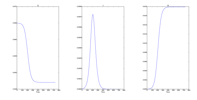
Figure 2: Solution of a simple SIR model

Epidemiology focused features

PyGOM can decompose a set of ODEs into individual transitions between states and birth/death processes. Consider a simple vector–host SIS model [2]

$$S_{h}^{\prime} =\lambda_{h}+\mu_{h}S_{h}-\beta_{h}S_{h}I_{v}+\gamma I_{h}$$

$$S_{v}^{\prime} =\lambda_{v}+\mu_{v}S_{v}-\beta_{v}S_{v}I_{h}$$

$$I_{h}^{\prime} =\beta_{h}S_{h}I_{v}-(\mu_{h}+\gamma)I_{h})$$

$$I_{v}^{\prime} =\beta_{v}S_{v}I_{h}-\mu_{v}I_{v},$$

under Lagrange’s notation. This can be entered into PyGOM as

⬇

>>> from pygom import SimulateOde, Transition as T

>>> state = [’S_v’, ’S_h’, ’I_v’, ’I_h’]

>>> param = [’beta_v’, ’beta_h’, ’mu_v’, ’mu_h’,

’lambda_v’, ’lambda_h’, ’gamma’]

>>> t1 = T(’S_h’, ’lambda_h-mu_h*S_h-beta_h*S_h*I_v+gamma*I_h’)

>>> t2 = T(’S_v’, ’lambda_v-mu_v*S_v-beta_v*S_v*I_h’)

>>> t3 = T(’I_h’, ’beta_h*S_h*I_v-(mu_h+gamma)*I_h’)

>>> t4 = T(’I_v’, ’beta_v*S_v*I_h-mu_v*I_v’)

>>> ode = SimulateOde(state, param, ode=[t1,t2,t3,t4])

where the last line initializes the model. Some of the standard operations such as simulating the ODE can be performed and will be discussed later.

We show how an R0 can be obtained by calling the corresponding methods, given the disease states as per the second line below.

⬇

>>> from pygom.model.epi_analysis import R0

>>> ode = ode.get_unrolled_obj()

>>> R0(ode, [’I_v’,’I_h’])

sqrt(beta_h*beta_v*lambda_h*lambda_v/(mu_h*(gamma+mu_h)))/Abs(mu_v)

The R0 value above has already made the substitution for the states using the disease free equilibrium (DFE). Algebraic expression for the DFE can be obtained on its own, and the output would have been numerical instead of symbolic if the parameter values were available. Note that the ode object has been replaced in the first line and is now composed of transitions between states and birth/death processes. We can visualize the model or perform manipulation (such as deleting a death process) with this new object.

In depth usage

Transitions and the transition object

Fundamental to setting up a model is to correctly define the set of ODEs that are to be built into the system. Within PyGOM these are defined using the Transition object defined in the transition module. The construction of such an object takes a number arguments but the four most important ones are:

1. The origin state (origin)

2. An equation, as a string, that defines the process (equation)

3. The type of transition (transition_type)

4. The destination state (destination)

When constructing a Transition object, two arguments are required with two optional arguments: transition_type, destination, defaulting to an ’ode’ and None. While we have only showed a transition between two states, both the origin and destination can accommodate multiple states to represent transitions like $A+A\rightarrow B+C$. In the example above we showed that the SIR model could be constructed using either the equations of the transition between states using a Transition with type T, or by defining the ODEs that control the states using a transition of type ODE. Two further types of transitions are possible, birth and death processes, which are types B and D respectively. These add to or remove from a state without a source or destination state.

Defining the model through a class structure is no more difficult than say MATLAB or Python in their plain equation form. Although some of the code samples shown here appear to be more cumbersome when compared to simply writing it out in other programming languages, this only holds when trying to define the model using different types of transitions. It can be seen above that an end user can almost view it as writing the model as they would in MATLAB, by replacing the equality sign with initialization of Transition object.

All birth and death processes can be added to the model at any time, given that the corresponding parameters exist in the model object. Below, in the first six commands, we add three birth/death processes to the original SIR model, add the additional birth rate parameter and redefine the time–line. These operations and setting the value of the new parameters can be done without referring to information previously defined. The last line of the code simply recomputes the solution given our new system, and the corresponding plot in Fig. 3.

⬇

>>> bdList = [Transition(origin=’S’,

equation=’B’,

transition_type=TransitionType.B),

Transition(origin=’S’,

equation=’mu*S’,

transition_type=TransitionType.D),

Transition(origin=’I’,

equation=’mu*I’,

transition_type=TransitionType.D)]

>>> B = 126372.0/365.0

>>> t = np.linspace(0,35*365,10001)

>>> model.param_list = [’B’, ’mu’]

>>> model.birth_death_list = bdList

>>> model.parameters = {’B’:B,’mu’:B/N}

>>> solution = model.integrate(t[1::])

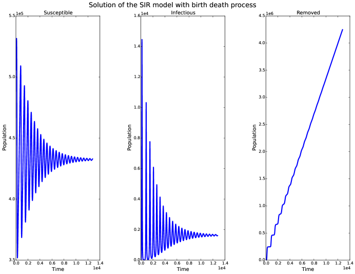
Figure 3: Solution of the SIR model over time with birth death processes that induce oscillations

An important point to consider is how the information regarding the construction of ODEs is provided to DeterministicOde at initialization. For ODEs the transition list is provided to the ode argument, for transitions to the transition argument and for birth and deaths it is to the birth_death argument. DeterministicOde will raise an error if an incorrectly typed transition is presented to these arguments. PyGOM has been constructed in this way to capture common errors in model specification and to help ensure that transitions are defined carefully. An ODE system may be constructed with a mixture of transition types so long as the transitions are placed in the correct list.

Stochastic simulation

There are situations when we are less interested in just a single deterministic solution to a model with given parameters, but in a set of possible realizations given the variation and uncertainty in many natural systems. In such cases, we are interested in the stochastic behavior of a model. There are two common ways to introduce stochasticity to a model

1. Take parameter values as realizations from a random process.

2. Drive changes between states using a probabilistic jump process.

PyGOM is capable of generating realizations for either of these two scenarios. Moreover, the manner in which a model is defined changes very little from the deterministic case already discussed. If the library dask is installed, PyGOM will automatically generate realizations in parallel.

Parameter stochasticity

When we wish to use the first type of stochasticity our parameter values are drawn from an underlying distribution. For the SIR model to be biologically meaningful it is clear that both $\beta$ and $\gamma$ must be non–negative, so it would seem natural to use the gamma distribution. Some of the more commonly used distributions are provided within the utilR sub–package, where we have used the R language [24] naming conventions for the distribution names and input argument. Users are free to use functions from scipy’s stats sub–module or any other arbitrary function that is callable with the number of realizations as the first input argument followed by the distribution parameters.

We define a stochastic model in a very similar way to the previous models, indeed we can reuse the setup for the deterministic model defined above

⬇

>>> from pygom import SimulateOde

>>> modelS = SimulateOde(states,

params,

transition=[sir_t1, sir_t2])

Now we define and set the parameters. We can use a mix of stochastic and non–stochastic parameters, if required, as shown below, where the total population $N$ is a constant in this case and the birth and death processes from above have been removed. Here we define the parameters in a Python dictionary (d). Each parameter in the model is a key in this dictionary with the value either as a constant or as a tuple containing the generating function and a dictionary with the generating function’s attributes

⬇

>>> from pygom.utilR import rgamma

>>> d = dict()

>>> d[’beta’] = (rgamma, {’shape’:3600.0, ’rate’:1000.0})

>>> d[’gamma’] = (rgamma, {’shape’:1000.0, ’rate’:5000.0})

>>> d[’N’] = N

>>> modelS.parameters = d

>>> init_state = [int(i) for i in init_state]

>>> modelS.initial_values = (init_state, t[0])

We generate 10 realizations (iteration=10) from this model as an example and ask for the full output of the simulations via full_output=True

⬇

>>> Ymean, Yall = modelS.simulate_param(t,

iteration=10,

full_output=True)

The output from this simulation will be a tuple with the first element containing the sample mean and the second a list of solutions. Here we have simply split the tuple on assignment into Ymean and Yall. The values in the Yall variable permit the user to construct an empiric predictive interval and, by plotting the values in the Yall variable, we may visualize the results of the simulation as in Fig. 4.

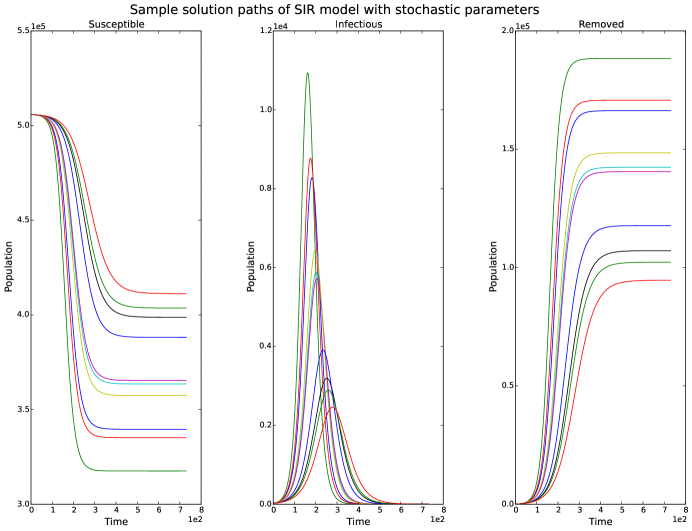
Figure 4: Results, by compartment, of 10 realizations of a stochastic SIR model

Jump processes or master equation stochasticity

Compared to the example above where we assume that movements between states are small and continuous, in this method of introducing stochasticity to an ODE system we assume that movements between states are discrete, termed jumps. More concretely, the probability of a move for transition $j$ is governed by an exponential distribution such that

$$\Pr(\textnormal{process $j$ jump within time }\tau)=\lambda_{j}e^{-\lambda_{j}\tau}$$

where $\lambda_{j}$ is the rate of transition for process $j$ and $\tau$ the time elapsed after current time $t$. In chemistry and physics this known as a master equation model. Greater detail of these systems and their solutions may be found in [12]. We first reset the parameters so that they are fixed rather than stochastic

⬇

>>> modelS.parameters = param_eval

>>> t_jump = np.linspace(0,100,50)

We then perform a set of jump process simulations, this is similar to parameter stochasticity simulation, differing only in the name of the method invoked

⬇

>>> simX, simT =modelS.simulate_jump(t_jump,

iteration=10,

full_output=True)

As before we can use the result variables with a graphics package to produce a visualization of these simulations as in Fig. 5. Simulation results are approximate as they are performed using the $\tau$–Leap algorithm [3] by default, with the options of obtaining an exact simulation [11] if desired.

Here we have “zoomed” into a section of the time points compared to previous Figures. This is because the jumps occur on a much smaller time scale, and indeed both the S and R state appears to be smooth with discontinuity observed in only the I state.

Unlike any of the previous models a jump process model is able to produce simulations where the disease is completely eliminated from the model before the disease has run its full course (all members of the ‘I’ compartment moved to ‘R’ before more individuals become infected). You can see the result of this in Fig. 5 as the horizontal lines at the top of the susceptible graph and at the bottom of the removed graph.

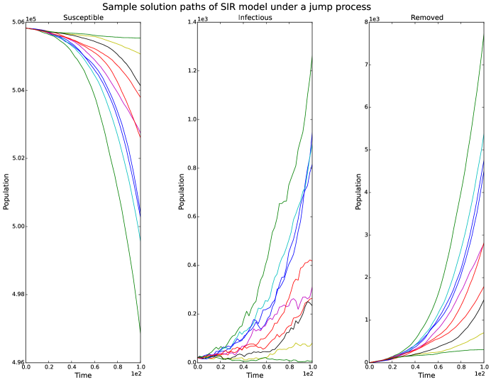
Figure 5: Ten simulated paths under a continuous time Markov process.

Parameter estimation and testing model fit

Given an observational data set relating to a system being modeled we may wish either to test an ODE based model to see how well it fits the data or use the data to estimate the parameter values within the system. Were we to have a set of $n$ observations $y_{i}$ at specific time points $t_{i}$, $i=1,\ldots,n$ we would require a function that measures the disparity between this data and the model, a loss function. Within PyGOM we have implemented the most common loss functions in the ode_loss module. Of particular note is the square loss (squared error) $\left\|\mathbf{y}-\hat{\mathbf{y}}\right\|^{2}$ function which we use in the following examples. Square loss is also the simplest and most commonly used loss function. PyGOM also provides parametric loss functions via the Poisson and Normal distributions.

All our loss functions come with the ability to return the cost, amount of loss incurred with respect to the data, as well as the residuals which are essential to post–estimate analysis such as tests for normality and autocorrelation. These loss classes take multivariate observations, i.e. $\mathbf{y}$ is a matrix of size $\left[n\times k\right]$ where $n$ is the number of observations and $k$ the number of targeted states. Furthermore, under the square or normal loss functions, it is possible to set weights on the observations. The weights may be scalar or vector, with size equal to the number of targeted states or observations.

Parameter estimation is a non–linear optimization problem which has been tackled by both deterministic and stochastic estimation methods [1]. That is, we seek a set of parameter values that minimize the loss function. Our focus here is on obtaining the derivatives information as they are central in deterministic methods, and have been shown to be useful in the stochastic setting such as Monte Carlo Markov chain [13].

We reuse the SIR model above, but this time initialized using the pre–defined version in the common_models sub–module of PyGOM. Note how easy it is to use a completely different set of parameters, and with the corresponding $x_{0}$ and $\mathbf{t}$, we are ready to solve the IVP. The solution given fixed parameters can be viewed as observational data with perfect information. Here, we scale the solution of the R states by a random multiplier to ensure that the problem is non–trivial and take the result as our observed data

⬇

>>> from pygom import SquareLoss, common_models

>>> model = common_models.SIR({’beta’:0.5,’gamma’:1.0/3.0})

>>> init_state = [1,1.27e-6,0]

>>> model.initial_values = (init_state, t_jump[0])

>>> solution = model.integrate(t_jump[1:])

>>> y = solution[1:, -1]

>>> y = y * (0.90 + np.random.rand(len(y))/5.0)

Using this pseudo–data, the ODE object, our time and initial state vectors, we now construct a square loss object with an initial guess for the parameters $\beta$ and $\gamma$, in theta below.

⬇

>>> theta = [0.5,0.5]

>>> obj_sir = SquareLoss(theta=theta,

ode=model,

x0=init_state,

t0=t_jump[0],

t=t_jump[1:],

y=y,

state_name=[’R’])

In the example above we are looking at the entire parameter set (both $\beta$ and $\gamma$) but only through values observed in the ’R’ state. However, it is perfectly possible to target only specific parameters instead of the full set by specifying them through target_param and to include other state values through state_name.

We are going to put some constraints on the parameter space where we think the optimal parameter value may lie. This is necessary for the SIR model because the parameters must be non–negative, as per model definition. So, we bound the value for both parameters to between $0$ and $2$. These bounds are specified in the same order as the parameters were constructed above.

⬇

>>> bounds = [(0.0, 2.0), (0.0, 2.0)]

In the following example we use the default optimization method from scipy.optimize, with the gradient obtained from forward sensitivity

⬇

>>> from scipy.optimize import minimize

>>> theta_hat = minimize(fun=obj_sir.cost,

jac=obj_sir.sensitivity,

x0=[0.5, 0.5],

bounds=bounds)

In the result object the x gives the estimated parameter values. Here the estimates were $\beta=0.48427416,\gamma=0.31797725$.

To visualize the goodness–of–fit a plot method has been implemented within the loss function class. This may be invoked by simply calling the plot() method. Fig. 6 was generating using this convenience method which plots the observed values against the solutions generated by the best–fit parameters

⬇

>>> obj_sir.plot()

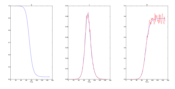
Figure 6: An example of the plot method from our loss classes. The red line is the observational data and the blue in all panels are the simulated paths with parameters as fitted.

Derivative Information

As seen above we made use of the loss function’s gradient when estimating the unknown parameters. PyGom’s loss functions provide two ways to calculate this gradient: sensitivity and adjoint, see 2.2 and 2.3 of [6] for details. The gradient function by default is a synonym for sensitivity. Substituting adjoint in place of sensitivity in the optimization above only has impact on the computational speed, which depends on the properties of the ODEs and we refer interested readers to [20, 6].

⬇

>>> S = obj_sir.sensitivity(theta)

>>> A = obj_sir.adjoint(theta)

Additionally, Hessian information is also available via hessian. The Hessian for a non–linear problem is not guaranteed to be a positive semi–definite matrix, hence certain algorithms such as the Levenberg–Marquardt algorithm only uses the approximation of the Hessian $\boldsymbol{H}\approx\boldsymbol{J}^{\top}\boldsymbol{J}$ where $\boldsymbol{J}$ is the Jacobian. This is also available via

⬇

>>> J = obj_sir.jac(theta)

Note that when $y$ is a multivariate observation, the return by residual is a matrix and jac is a matrix with $np$ (number of observations $\times$ number of parameters) columns. If the approximation is required instead of just the Jacobian, it can be obtained using

⬇

>>> JTJ = obj_sir.jtj(theta)

Confidence Interval of Estimated Parameters

After obtaining the best fit value for a parameter, it is natural to report both the point estimate and the confidence level at a given $\alpha$ (the false positive or Type I error rate, typically $5\%$). Within PyGOM we provide several methods to calculate such a confidence interval and describe three in detail below.

Asymptotic

The simplest method of calculating a confidence interval is to invoke the normality argument and use the Fisher information of the likelihood [4]. From the Cramér–Rao inequality we know that

$$\textnormal{Var}(\hat{\theta})\geq\frac{1}{I(\theta)}$$

where $I(\theta)$ is the Fisher information, which we take as the Hessian. The normality comes from invoking the central limit theorem. Obtaining an estimate of this confidence interval with PyGOM is as simple as defining our significance level $\alpha$, calculating our fit and determining the interval.

⬇

>>> from pygom import confidence_interval as ci

>>> alpha = 0.05

>>> xLower, xUpper = ci.asymptotic(obj=obj_sir,

alpha=alpha,

theta=theta_hat[’x’])

>>> print(xLower)

[ 0.21941127 0.07131115]

>>> print(xUpper)

[ 0.74913705 0.56464335]

The xLower and xUpper objects now contain the lower and upper bounds for the parameters. As before with the fits, the parameter order is the same as was specified when the model was created.

Profile and Geometric likelihood

Another approach to calculating the confidence intervals is to take each parameter individually, treating the remaining parameters as nuisance variables, hence the term profile. We provide a function within the confidence_interval module to obtain such an estimate, profile. The solving of the system of equations for profile likelihood requires only Newton like steps, possibly with correction terms as per [32]. However, this is usually hard or even impossible for ODE systems because the likelihood is not monotonic either side of the central parameter estimate. This is typically caused by a lack of observations, and is therefore not an issue which an end user is able to address. In the face of this we provide an alternative way to generate a result similar to profile likelihood using the geometric structure of the likelihood. We follow the method in [23], which involves solving a set of differential equations. The confidence interval is obtained by solving an IVP from $t=0$ to $1$ and is all handled internally via the geometric() function in PyGOM’s confidence_interval module. A more in–depth exposition of these types of likelihood estimation is provided in the supplementary material in S4.

⬇

>>> xLGeometric, xUGeometric = ci.geometric(

obj=obj_sir,

alpha=alpha,

theta=theta_hat[’x’])

>>> print(xLGeometric)

[ 0.21371156 0.05306822]

>>> print(xUGeometric)

[ 0.97617977 0.77965589]

Bootstrap confidence intervals

Bootstrap estimation [8] is a widely favored technique for estimating confidence intervals. There exist many implementations of bootstrap. A semi–parametric method seems to be the most logical choice within the context of ODEs (even when the assumptions are violated at times). When we say semi-parametric, we mean the exchange of errors between the observations. Let our raw error be

$$\varepsilon_{i}=y_{i}-\hat{y}_{i}$$

where $\hat{y}_{i}$ will be the prediction under $\hat{\boldsymbol{\theta}}$ in our model. Then we construct a new set of observations via

$$y_{i}^{\ast}=\hat{y}_{i}+\varepsilon^{\ast},\quad\varepsilon^{\ast}\sim\mathcal{F},$$

with $\mathcal{F}$ being the empirical distribution of the raw errors. As with the previous confidence interval methods bootstrap from the confidence_interval module will calculate this type of confidence interval.

⬇

>>> xLBootstrap, xUBootstrap = ci.bootstrap(obj=obj_sir,

alpha=alpha,

theta=theta_hat[’x’],

iteration=100,

lb=bounds_arr[:,0],

ub=bounds_arr[:,1])

>>> print(xLBootstrap)

[ 0.47400253 0.30820995]

>>> print(xUBootstrap)

[ 0.49925899 0.33143419]

The bounds should be specified whenever possible because they are used when estimating the parameters for all of the bootstrap samples. An error will be returned and terminate the whole process whenever the estimation process is not successful. All the bootstrap estimates can be obtained by setting full_output=True, and they can be used to compute the bias, tail effects and for tests of the normality assumption. If desired, a simultaneous confidence interval can also be approximated empirically. Note however that because we are using a semi–parametric method here, if the model specification is wrong then the resulting information is also wrong. The confidence interval will still have the normal approximation guarantee if the number of samples is large. As bootstrap confidence intervals follow an empiric distribution we do not expect them to match those produced by the parametric types. In this case, because the error in the observation is extremely small we find that the confidence interval is narrower.

The PyGOM package

Availability and Installation

The source code for this package is available on GitHub and through the Python Package Index (PyPI). As such, it may be easily installed via pip: pip install pygom

Dependencies

Our package depends on most of the core SciPy libraries. This includes SciPy, Numpy, Matplotlib and Sympy. Additional dependencies may be required, which depends on the level of functionality the end user desires. For example, parallel stochastic simulation occurs if dask has been installed, and displaying transition diagrams requires graphviz.

Conclusion

To summarize, PyGOM is designed to simplify the construction of ODE based models, with a bias towards modeling epidemiology that can: decomposing a set of ODEs, obtaining epidemic related measures such as R0, perform parameter estimation with high quality confidence intervals. This package is free and will always be free. Generic operations found for all types of ODE modeling are available and plans to appeal to a wider audience by say integrating with the SBML specification are underway.

Our intention was to make the definition of ODE based model systems easy while maintaining rigor within that definition. This was to allow the rapid assessment of published model systems and results in the absence of source code. PyGOM has grown beyond that original idea into a comprehensive toolbox which includes tools that make common operations on such systems, such as solving for a series of time–points or fitting parameters to data, simple. In addition to this software, within the common_models module we have collected and implemented many common reference ODE systems as a foundation for the user to construct new models or fit canonical models to new data. To aid the newcomer to PyGOM, in addition to this paper included with the package there is an extensive manual for PyGOM with further worked examples.

From the outset, the PyGOM package has been designed to be modular and extensible. Starting with a small core of useful abilities, this modular architecture has allowed new functionality to be added to the package without requiring adjustments to existing code. Its modularity also helps keep the code maintainable and comprehensible. Planned enhancements to the package will seek to account for non–identifiability when parameter values are being estimated and further assistance in the algebraic analysis of the ODE system.

As a system published under an Open License with the code freely available to all, PyGOM fits well into the ever–expanding universe of Open Source analysis tools. This openness permits the data–scientist to use PyGOM in conjunction with other analysis libraries within Python as well as more widely with other open–source tools such as those in R; and in environments ranging from single machines through to large clusters and machine clouds.

By making common operations easy for the end user, we free them to use the knowledge of their domain to construct and explore ODE–based model systems without needing complex or esoteric computer code, leaving to the computer the tedious tasks of book keeping and mathematical transformation. Even amongst professional mathematicians and modelers PyGOM greatly simplifies and speeds up the modeling process as it provides tools that allow easy construction of robust work–flows, with validation and visualization aids built in. Together these features allow the user to concentrate on the model.

References

- [1] Julio R. Banga, Carmen G. Moles, and Antonio A. Alonso. Global Optimization of Bioprocesses using Stochastic and Hybrid Methods. In C. A. Floudas and Panos Pardalos, editors, Frontiers in Global Optimization, number 74 in Nonconvex Optimization and Its Applications, pages 45–70. Springer US, 2004.
- [2] Fred Brauer, Pauline van den Driessche, and Jianhong Wu. Mathematical Epidemiology. Springer Berlin Heidelberg, 2008.
- [3] Yang Cao, Daniel T. Gillespie, and Linda R. Petzold. Efficient step size selection for the tau-leaping simulation method. The Journal of chemical physics, 124(4):044109, January 2006.
- [4] George Casella and Roger L. Berger. Statistical Inference. Duxbury Press, 2 edition, 2001.
- [5] Simon Cauchemez, Christophe Fraser, Maria D. Van Kerkhove, Christl A. Donnelly, Steven Riley, Andrew Rambaut, Vincent Enouf, Sylvie van der Werf, and Neil M. Ferguson. Middle East respiratory syndrome coronavirus: quantification of the extent of the epidemic, surveillance biases, and transmissibility. The Lancet. Infectious Diseases, 14(1):50–56, January 2014.
- [6] Guy Chavent. Nonlinear Least Squares for Inverse Problems: Theoretical Foundations and Step-by-Step Guide for Applications. Springer Netherlands, 2010.
- [7] Earl E. Coddington. Theory of Ordinary Differential Equations. Krieger Pub Co, 1984.
- [8] A. C. Davison and D. V. Hinkley. Bootstrap Methods and Their Applications. Cambridge University Press, Cambridge, 1997. ISBN 0-521-57391-2.
- [9] Thomas J. R. Finnie, Andy South, Ana Bento, Ellie Sherrard-Smith, and Thibaut Jombart. EpiJSON: A unified data-format for epidemiology. Epidemics, 15:20–26, June 2016.
- [10] C. Fraser, C. A Donnelly, S. Cauchemez, W. P Hanage, M. D Van Kerkhove, T. D Hollingsworth, J. Griffin, R. F Baggaley, H. E Jenkins, E. J Lyons, et al. Pandemic potential of a strain of influenza A (H1n1): early findings. Science, 324(5934):1557, 2009.
- [11] Daniel T. Gillespie. Exact stochastic simulation of coupled chemical reactions. The Journal of Physical Chemistry, 81(25):2340–2361, 1977.
- [12] Daniel T. Gillespie. Stochastic simulation of chemical kinetics. Annual review of physical chemistry, 58:35–55, January 2007.
- [13] Mark Girolami and Ben Calderhead. Riemann manifold Langevin and Hamiltonian Monte Carlo methods. Journal of the Royal Statistical Society: Series B (Statistical Methodology), 73(2):123–214, 2011.
- [14] Ernst Hairer, S P Nørsett, and Gerhard Wanner. Solving Ordinary Differential Equations I: Nonstiff Problems. Springer Berlin Heidelberg, 2 edition, 1993.
- [15] Ernst Hairer and Gerhard Wanner. Solving Ordinary Differential Equations II: Stiff and Differential-Algebraic Problems. Springer Berlin Heidelberg, 2 edition, 1996.
- [16] John D. Hedengren, Reza Asgharzadeh Shishavan, Kody M. Powell, and Thomas F. Edgar. Nonlinear modeling, estimation and predictive control in apmonitor. Computers & Chemical Engineering, 70:133–148, November 2014.
- [17] Alan C. Hindmarsh, Peter N. Brown, Keith E. Grant, Steven L. Lee, Radu Serban, Dan E. Shumaker, and Carol S. Woodward. SUNDIALS. ACM Transactions on Mathematical Software, 31(3):363–396, September 2005.
- [18] M. Hucka, A. Finney, H. M. Sauro, H. Bolouri, J. C. Doyle, H. Kitano, and the rest of the SBML Forum, A. P. Arkin, B. J. Bornstein, D. Bray, A. Cornish-Bowden, A. A. Cuellar, S. Dronov, E. D. Gilles, M. Ginkel, V. Gor, I. I. Goryanin, W. J. Hedley, T. C. Hodgman, J.-H. Hofmeyr, P. J. Hunter, N. S. Juty, J. L. Kasberger, A. Kremling, U. Kummer, N. Le Novére, L. M. Loew, D. Lucio, P. Mendes, E. Minch, E. D. Mjolsness, Y. Nakayama, M. R. Nelson, P. F. Nielsen, T. Sakurada, J. C. Schaff, B. E. Shapiro, T. S. Shimizu, H. D. Spence, J. Stelling, K. Takahashi, M. Tomita, J. Wagner, and J. Wang. The systems biology markup language (SBML): a medium for representation and exchange of biochemical network models. Bioinformatics, 19(4):524–531, January 2003.
- [19] John Denholm Lambert. Computational methods in ordinary differential equations. Wiley-Blackwell, 1973.
- [20] Shengtai Li, Linda R. Petzold, and Wenjie Zhu. Sensitivity analysis of differential algebraic equations: A comparison of methods on a special problem. Applied Numerical Mathematics, 32(2):161–174, February 2000.
- [21] Thomas Maiwald and Jens Timmer. Dynamical modeling and multi-experiment fitting with potterswheel. Bioinformatics (Oxford, England), 24(18):2037–43, September 2008.
- [22] Andrew K. Miller, Justin Marsh, Adam Reeve, Alan Garny, Randall Britten, Matt Halstead, Jonathan Cooper, David P. Nickerson, and Poul F. Nielsen. An overview of the CellML API and its implementation. BMC Bioinformatics, 11:178, 2010.
- [23] Suresh H. Moolgavkar and David J. Venzon. Confidence regions for parameters of the proportional hazards model: A simulation study. Scandinavian Journal of Statistics, 14(1):43–56, 1987.
- [24] R Core Team. R: A Language and Environment for Statistical Computing. R Foundation for Statistical Computing, Vienna, Austria, 2014.
- [25] James C. Robinson. An Introduction to Ordinary Differential Equations. Cambridge University Press, 2004.
- [26] Henning Schmidt and Mats Jirstrand. Systems biology toolbox for matlab: a computational platform for research in systems biology. Bioinformatics (Oxford, England), 22(4):514–5, February 2006.
- [27] Lucian P. Smith, Erik Butterworth, James B. Bassingthwaighte, and Herbert M. Sauro. SBML and CellML translation in Antimony and JSim. Bioinformatics, 30(7):903–907, January 2014.
- [28] K. A. Stroud and Dexter Booth. Differential Equations. Industial Press, 2004.
- [29] SymPy Development Team. SymPy: Python library for symbolic mathematics, 2014.
- [30] WHO Ebola Response Team. Ebola Virus Disease in West Africa — The First 9 Months of the Epidemic and Forward Projections. New England Journal of Medicine, 371(16):1481–1495, October 2014.
- [31] WHO Ebola Response Team. West African Ebola Epidemic after One Year — Slowing but Not Yet under Control. New England Journal of Medicine, 372(6):584–587, February 2015.
- [32] D. J. Venzon and S. H. Moolgavkar. A method for computing profile-likelihood-based confidence intervals. Journal of the Royal Statistical Society. Series C (Applied Statistics), 37(1):87–94, 1988.