On the Keldysh Problem of Flutter Suppression

Abstract

This work is devoted to the Keldysh model of flutter suppression and rigorous approaches to its analysis. To solve the stabilization problem in the Keldysh model we use an analog of direct Lyapunov method for differential inclusions. The results obtained here are compared with the results of Keldysh obtained by the method of harmonic balance (describing function method), which is an approximate method for analyzing the existence of periodic solutions. The limitations of the use of describing function method for the study of systems with dry friction and stationary segment are demonstrated.

1 INTRODUCTION

The notion of flutter is traced back to the work of Lanchester [1], where torsional vibrations of the tail of Handley Page 0/400 biplane bomber were described. Flutter is a self-excited oscillation, often destructive, wherein energy is absorbed from the airstream; it is a complex phenomenon that must in general be completely eliminated by design or prevented from occurring within the flight envelope [2]. In the work by Parhomovsky and Popov [3] it is remarked that about 150 crashes of new models of aircrafts caused by flutter happened in German aviation during 1935-1943, while in the Soviet Union the works of M.V. Keldysh and his scientific school in TsAGI allowed to avoid the numerous accidents that accompanied the development of aviation. In this work we revisit the work by M.Keldysh on the flutter suppression by dampers with a nonlinear characteristic, published in 1944 [4].

2 KELDYSH PROBLEM ON THE FLUTTER SUPPRESSION

Follow [4], first we consider the suppression of flutter for a model with one degree of freedom

$$J\ddot{x}+kx=(-\lambda+h)\dot{x}-\varphi(\dot{x}),\quad\varphi(\dot{x})=(\Phi+\kappa\dot{x}^{2}){\rm sign}(\dot{x}),$$ (1)

where $J>0$ — the moment of inertia, $k>0$ — stiffness, $h\dot{x}$ — an excitation force proportional to the angular velocity $\dot{x}$, $f(\dot{x})=\lambda\dot{x}+\varphi(\dot{x})$ — nonlinear characteristic of hydraulic damper with dry friction, $\Phi$ — the dry friction coefficient, $\lambda>0$ and $\kappa>0$ — parameters of the hydraulic damper. Following the mechanical sense, Keldysh defined ${\rm sign}(0)$ as a value from $[-\Phi,\Phi]$ and, thus, the discontinuous differential equation (1) has a segment of equilibria (stationary segment).

Let $\mu=\lambda-h.$ Using the describing function method (DFM, harmonic balance), which had been well developed by 1944 [5], Keldysh formulated the following result:

1. If

   $$-2.08\sqrt{\Phi\kappa}<\mu,$$ (2)

   then all trajectories of (1) converge to the stationary segment;

2. If

   $$\mu<-2.08\sqrt{\Phi\kappa},$$ (3)

   then there are two periodic trajectories (limit cycles) $\approx a_{\pm}\cos(\omega t)$ with amplitudes

   $$a_{\pm}(\mu)=\frac{3}{8\kappa}\sqrt{\frac{J}{k}}\bigg{(}\pi(\mu)\pm\sqrt{\pi^{2}(\mu)^{2}-\frac{32}{3}\kappa\Phi}\bigg{)}.$$

   Other trajectories behave as follows. The trajectories, emerging from infinity, tend to the external limit cycle. The domain between two limit cycles is filled with trajectories unwinding from the internal (unstable) limit cycle and winding onto external (stable) limit cycle. The stability domain bounded by the internal limit cycle is filled with trajectories tending to one of the possible equilibrium on the stationary segment.

It is well known that the classical DFM is only an approximate method which gives the information on the frequency and amplitude of periodic orbits and, in general, may lead to wrong conclusions about the existence of periodic orbits. In his paper [4] Keldysh wrote: “we do not give a rigorous mathematical proof …, we construct a number of conclusions on intuitive considerations …”.

Nowadays we can apply rigorous analytical and reliable numerical methods, which have been developed from 1944 till now: theory of differential inclusions (see, e.g. [16, 17]); direct Lyapunov method and frequency methods (see, e.g. [18, 17, 19]); numerical algorithms for solving differential inclusions (see, e.g. [20, 21, 22]). Follow the theory of differential inclusion, for the model (1) we consider the discontinuity manifold: $S=\{\dot{x}\!:\ \dot{x}=0\}$ on the phase space $(x,\dot{x})$, define $\varphi(\dot{x})$ on $S$ as the set $[-\Phi,+\Phi]$, and get differential inclusion

$$J\ddot{x}+kx+\mu\dot{x}\in-\hat{\varphi}(\dot{x}),\quad\hat{\varphi}(\dot{x})=\left\{\begin{array}[]{lc}\varphi(\dot{x})&\dot{x}\neq 0,\cr[-\Phi,+\Phi]&\dot{x}=0.\end{array}\right.$$ (4)

The solutions of (4) are considered in the sense of Filippov [16]. Remark that here solutions cannot slide on the discontinuity manifold $S$, but can tend to the stationary segment:

$$\Lambda=\{\ -\Phi/k\leq x\leq\Phi/k,\dot{x}=0\}\subset S,$$

or pierce the manifold $S\backslash\Lambda$.

Theorem 1. If

$$-2\sqrt{\Phi\kappa}<\mu,$$ (5)

then any solution of (4) converges to the stationary segment $\Lambda$.

Proof sketch. Consider Lyapunov function

$$V(x,\dot{x})=\frac{1}{2}(J\dot{x}^{2}+kx^{2}).$$

Since $\dot{x}\varphi(\dot{x})>0$ for $\dot{x}\neq 0$, we have

$$\dot{V}(x,\dot{x})=-\mu\dot{x}^{2}-\dot{x}\varphi(\dot{x})<0,\quad\forall\dot{x}\notin S.$$

The equality $V(x(t),\dot{x}(t))\equiv{\rm const}$ can hold only for $x\in\Lambda$. By the analog direct Lyapunov method for differential inclusions [17, Lemma 1.5, p.58] we get the assertion of the theorem. $\blacksquare$

Thus, rigorous analytical estimate (5) is close to Keldysh’s estimate of the global stability region (2): $\delta_{0}=2\sqrt{\Phi\kappa}<2.8\sqrt{\Phi\kappa}=\delta_{K}.$

Next, we consider Keldysh’s estimate of the bounded stability region (3) and demonstrate the difficulties of the DFM application to the systems with dry friction and stationary segment. To simplify numerical simulation of (4) we use the following transformations: $x\to\frac{J}{\kappa}x,t\to t\frac{\sqrt{J}}{\sqrt{k}}\ \Rightarrow\ J=1,k=1,\kappa=1.$

Fig. 1 shows qualitative behavior of trajectories on the phase space in the case of multistability and coexistence of two limit cycles for $\mu<-\delta_{K}$. Here the external limit cycle is a hidden attractor and corresponds to the flutter. The basin of attraction of the stationary segment $[-\Phi,\Phi]$ is bounded by the internal unstable limit cycle. When the harmonic approximation $a_{-}\cos(t)$ of the unstable limit cycle has the amplitude $a_{-}<\Phi$, the stiffness of the model in vicinity of the ends of the stationary segment complicates the modeling (the right subfigure of Fig. 1).

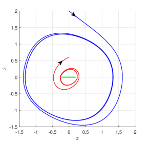
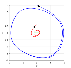
Figure 1: Numerical experiment with $\Phi=0.2$. Outer trajectory winds onto stable limit cycle, inner trajectory unwinds from unstable limit cycle and winds onto the stable limit cycle (hidden attractor). Left subfigure: $\mu\!=\!-1.3967\delta_{\!K}\!\!:a_{+}(\mu)\!>\!\!>\!a_{-}(\mu)\!>\!\Phi$. Right subfigure: $\mu\!=\!-1.7847\delta_{\!K}\!\!:a_{+}(\mu)\!>\!\!>\!\Phi\!>\!a_{-}(\mu)$.

Fig. 2 shows the bifurcation of collision of the external limit cycle and the stationary segment. In this numerical experiment both limit cycles have disappeared, while Keldysh’s estimate (3) holds.

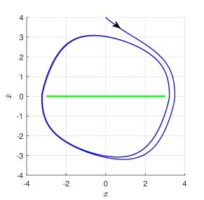
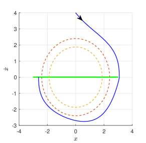
Figure 2: Numerical experiment with $\Phi\!=\!3$. Left subfigure: $\mu=-1.0713\delta_{K}$, $a_{+}(\mu)\gtrapprox\Phi>a_{-}(\mu)$; outer trajectory winds onto stable limit cycle, internal unstable limit cycle is not revealed numerically (due to stiffness). Right subfigure: $\mu=-1.0076\delta_{K}$, $\Phi\gtrapprox a_{+}(\mu)>a_{-}(\mu)$ (dash circles); outer trajectory approaches the stationary segment, both limit cycles have disappeared.

Thus, Keldysh’s estimate of the stability domain may be far from the numerical estimates.

3 CONCLUSIONS

Similar model with two degrees of freedom, considered by Keldysh in his paper [4], can be rigorously studied in the same way. For this case, the existence of the Lyapunov function and stability in large can be effectively proved by special frequency criteria [23]. Nowadays the study of stability in large and oscillations for modern aircrafts is also motivated by such problems as pilot induced oscillations and actuator saturations (see, e.g. surveys [24, 25] and references within). A terrifying illustration of such effects is the YF-22 crash in April 1992 and Gripen crash in August 1993 [26, 27]. In these regards, in the work [28] it is written that “since stability in simulations does not imply stability of the physical control system, stronger theoretical understanding is required”.

4 ACKNOWLEDGMENTS

Authors would like to thank Olga F. Radzivill (TsAGI Library), Boris R. Andrievsky (IPME RAS). This work was supported by the grant NSh-2858.2018.1 for the Leading Scientific Schools of Russia (2018-2019).

References

- Lanchester [1916] F. Lanchester, Torsional vibrations of the tail of an aeroplane (Aeronautical. Research Committee, Reports and Memoranda, 1916) , pp. 457–460.
- Garrick and Reed [1981] I. Garrick and W. Reed, Journal of Aircraft 18, 897–912 (1981).
- Parhomovsky and Popov [1971] Y. Parhomovsky and L. Popov, Tr. TsAGI (in Russian) II, 4–7 (1971).
- Keldysh [1944] M. Keldysh, Tr. TsAGI (in Russian) 557, 26–37 (1944).
- Krylov and Bogolyubov [1937] N. Krylov and N. Bogolyubov, Introduction to non-linear mechanics (in Russian) (AN USSR, Kiev, 1937) (English transl: Princeton Univ. Press, 1947).
- Aizerman [1949] M. A. Aizerman, Uspekhi Mat. Nauk (in Russian) 4, 187–188 (1949).
- Kalman [1957] R. E. Kalman, Transactions of ASME 79, 553–566 (1957).
- Bragin et al. [2011] V. Bragin, V. Vagaitsev, N. Kuznetsov, and G. Leonov, Journal of Computer and Systems Sciences International 50, 511–543 (2011).
- Leonov and Kuznetsov [2013] G. Leonov and N. Kuznetsov, International Journal of Bifurcation and Chaos 23 (2013), 10.1142/S0218127413300024, art. no. 1330002.
- Leonov et al. [2014] G. Leonov, N. Kuznetsov, M. Kiseleva, E. Solovyeva, and A. Zaretskiy, Nonlinear Dynamics 77, 277–288 (2014).
- Leonov et al. [2015] G. Leonov, N. Kuznetsov, M. Yuldashev, and R. Yuldashev, IEEE Transactions on Circuits and Systems–I: Regular Papers 62, 2454–2464 (2015).
- Kuznetsov [2016] N. Kuznetsov, Lecture Notes in Electrical Engineering 371, 13–25 (2016) .
- Dudkowski et al. [2016] D. Dudkowski, S. Jafari, T. Kapitaniak, N. Kuznetsov, G. Leonov, and A. Prasad, Physics Reports 637, 1–50 (2016).
- Kuznetsov et al. [2017] N. Kuznetsov, G. Leonov, M. Yuldashev, and R. Yuldashev, Commun Nonlinear Sci Numer Simulat 51, 39–49 (2017).
- Leonov et al. [2017] G. Leonov, N. Kuznetsov, M. Kiseleva, and R. Mokaev, Differential Equations 53, 1671–1697 (2017).
- Filippov [1988] A. F. Filippov, Differential equations with discontinuous right-hand sides (Kluwer, Dordrecht, 1988).
- Gelig, Leonov, and Yakubovich [1978] A. Gelig, G. Leonov, and V. Yakubovich, Stability of Nonlinear Systems with Nonunique Equilibrium (in Russian) (Nauka, 1978) (English transl: Stability of Stationary Sets in Control Systems with Discontinuous Nonlinearities, 2004, World Scientific).
- Lurie and Postnikov [1944] A. I. Lurie and V. N. Postnikov, Applied Mathematics and Mechanics (in Russian) 8, 246–248 (1944).
- Leonov, Ponomarenko, and Smirnova [1996] G. Leonov, D. Ponomarenko, and V. Smirnova, Frequency-Domain Methods for Nonlinear Analysis. Theory and Applications (World Scientific, Singapore, 1996).
- Aizerman and Pyatnitskiy [1974] M. Aizerman and E. Pyatnitskiy, Automation and Remote Control (in Russian) 7, 33–47, 8, 39–61 (1974).
- Dontchev and Lempio [1992] A. Dontchev and F. Lempio, SIAM Review 34, 263–294 (1992).
- Piiroinen and Kuznetsov [2008] P. T. Piiroinen and Y. A. Kuznetsov, ACM Transactions on Mathematical Software (TOMS) 34, p. 13 (2008).
- Leonov and Kuznetsov [2018] G. Leonov and N. Kuznetsov, Doklady Physics (2018), submitted.
- Leonov et al. [2012] G. Leonov, B. Andrievskii, N. Kuznetsov, and A. Pogromskii, Differential equations 48, 1700–1720 (2012).
- Andrievsky, Kuznetsov, and Leonov [2017] B. Andrievsky, N. Kuznetsov, and G. Leonov, Journal of Computer and Systems Sciences International 56, 455–470 (2017).
- Dornheim [1992] M. Dornheim, Aviation Week and Space Technology 137, 53–54 (1992).
- Shifrin [1993] C. Shifrin, Aviation Week and Space Technology 139, 78–79 (1993).
- Lauvdal, Murray, and Fossen [1997] T. Lauvdal, R. Murray, and T. Fossen, “Stabilization of integrator chains in the presence of magnitude and rate saturations: a gain scheduling approach,” in Proc. IEEE Control and Decision Conference, Vol. 4 (1997) , pp. 4404–4005.