Table Based Detection of Degenerate Predicates in Free Space Construction

Abstract.

The key to a robust and efficient implementation of a computational geometry algorithm is an efficient algorithm for detecting degenerate predicates. We study degeneracy detection in constructing the free space of a polyhedron that rotates around a fixed axis and translates freely relative to another polyhedron. The structure of the free space is determined by the signs of univariate polynomials, called angle polynomials, whose coefficients are polynomials in the coordinates of the vertices of the polyhedra. Every predicate is expressible as the sign of an angle polynomial $f$ evaluated at a zero $t$ of an angle polynomial $g$. A predicate is degenerate (the sign is zero) when $t$ is a zero of a common factor of $f$ and $g$. We present an efficient degeneracy detection algorithm based on a one-time factoring of every possible angle polynomial. Our algorithm is 3500 times faster than the standard algorithm based on greatest common divisor computation. It reduces the share of degeneracy detection in our free space computations from 90% to 0.5% of the running time.

1. Introduction

An implementation of a computational geometry algorithm is robust if for every input the combinatorial output is correct and the numerical output is accurate. The challenge is to implement the predicates in the algorithms: the signs of algebraic expressions whose variables are input parameters. A predicate is degenerate if its sign is zero. A nondegenerate predicate can usually be evaluated quickly, using machine arithmetic. However, detecting that a predicate is degenerate requires more costly computation.

We present research in degeneracy detection. Prior research mainly addresses degeneracy due to nongeneric input, such as the signed area of a triangle with collinear vertices. Such degeneracy is easily eliminated by input perturbation [3]. We address predicates, which we call identities, that are degenerate for all choices of the input parameters. One example is the signed area of a triangle $pab$ with $p$ the intersection point of line segments $ab$ and $cd$, which is identical to zero when $p$ is replaced by its definition in terms of the input. This identity occurs when constructing the convex hull of the intersection of two polygons. Figure 1 shows generic polygons $abc$ and $defgh$ that intersect at points $\{p_{1},\ldots,p_{6}\}$. The convex hull algorithm encounters an identity when it evaluates the signed area of any three of $\{p_{1},p_{2},p_{3},p_{4}\}$. Triangulating the intersection of two polygons involves similar identities.

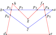
(a)	(b)	(c)

Figure 1. (a) Polygons, (b) intersection, and (c) convex hull.

Identities are common when the output of one algorithm is the input to another. The second algorithm evaluates polynomials (the signed area in our example) on arguments (the $p_{i}$ in our example) that are derived from input parameters by the first algorithm. When these algebraic expressions are rational, the identities are amenable to polynomial identity detection [9]. We are interested in identities involving more general algebraic expressions.

There are two general approaches to identity detection (Sec. 2). One [1] uses software integer arithmetic, computer algebra, and root separation bounds to detect all degenerate predicates, including identities. The second adds identity detection logic to computational geometry algorithms. In the convex hull example, this logic checks if three points lie on a single input segment. The first approach can greatly increase the running time of the software and the second approach can greatly increase the software development time.

We present a new approach to identity detection that avoids the high running time of numerical identity detection and the long development time of identity detection logic. The approach applies to a class of computational geometry algorithms with a common set of predicates. We write a program that enumerates and analyzes the predicates. The predicates are represented by algebraic expressions with canonical variables. The hull example requires 24 canonical variables for the coordinates of the at most 12 input points that define the three arguments of the signed area. When implementing the algorithms, we match their arguments against the canonical variables and use the stored analysis to detect identities.

We apply this approach in constructing the free space of a polyhedron $R$ that rotates around a fixed axis and translates freely relative to a polyhedron $O$ (Secs. 3 and 8). For example, $R$ models a drone helicopter and $O$ models a warehouse. The configuration of $R$ is specified by its position and its rotation angle. The configuration space is the set of configurations. The free space is the subset of the configuration space where the interiors of $R$ and $O$ are disjoint. Robust and efficient free space construction software would advance motion planning, part layout, assembly planning, and mechanical design.

The structure of the free space is determined by the configurations where $R$ has four contacts with $O$. A contact is determined by a vertex of $O$ and a facet of $R$, a facet of $O$ and a vertex of $R$, or an edge of $O$ and an edge of $R$. The angle (under a rational parameterization) of a configuration with four contacts is a zero of a univariate polynomial of degree 6, which we call an angle polynomial, whose coefficients are polynomials in the 48 coordinates of the 16 vertices of the 4 contacts. Every predicate in free space construction is expressible as the sign of an angle polynomial $f$ evaluated at a zero $t$ of an angle polynomial $g$ (Sec. 4). A predicate is degenerate when $t$ is a zero of a common factor $h$ of $f$ and $g$. It is an identity when $h$ corresponds to a common factor of $f$ and $g$ considered as multivariate polynomials in $t$ and in the vertex coordinates.

Neither prior identity detection approach is practical. Detecting an identity as a zero of the greatest common divisor of $f$ and $g$ is slow (Sec. 9). Devising identity detection logic for every predicate is infeasible because there are over 450,000,000 predicates and 13,000 identities (Sec. 7.4). We present an efficient identity detection algorithm (Sec. 6) based on a one-time analysis of the angle polynomials (Sec. 7).

We enumerate the angle polynomials using canonical variables for the vertex coordinates. Working in the monomial basis is impractical because many of the angle polynomials have over 100,000 terms. Instead, we represent angle polynomials with a data structure, called an a-poly, that is a list of sets of vertices (Sec. 5). The enumeration yields 1,000,000 a-polys, which we reduce to the 30,000 representatives of an equivalence relation that respects factorization. We construct a table of factors for the equivalence class representatives in one CPU-day on a workstation.

We factor an angle polynomial by looking up the factors of its representative in the table and substituting its vertex coordinates for the canonical variables. We use the factoring algorithm to associate each zero of an angle polynomial $g$ with an irreducible factor $h$. Before evaluating a predicate at $t$, we factor its angle polynomial $f$. The predicate is an identity if $h$ is one of the factors. Our algorithm is 3500 times faster than computing greatest common divisors. It reduces the share of degeneracy detection in our free space computations from 90% to 0.5% of the running time (Sec. 9). Sec. 10 provides guidelines for applying table-based identity detection to other domains.

2. Prior work

Identity detection is the computational bottleneck in prior work by Hachenberger [2] on computing the Minkowski sum of two polyhedra. He partitions the polyhedra into convex components and forms the union of the Minkowski sums of the components. Neighboring components share common, collinear, or coplanar features, resulting in many identities in the union operations. Detecting the identities via the numerical approach (using CGAL) dominates the running time.

Mayer et al [5] partially compute the free space of a convex polyhedron that rotates around a fixed axis and translates freely relative to a convex obstacle. They report no identity detection problems. Identities can be detected using one rule: all polynomials generated from a facet of one polyhedron and an edge of the other are the same up to sign and hence their zeros are identical. These polynomials correspond to our type I predicates for general polyhedra (Sec. 8).

We address identities in four prior works. We [4] compute polyhedral Minkowski sums orders of magnitude faster than Hachenberger by using a convolution algorithm, which has fewer identities, and by detecting identities with special case logic. We [6] compute free spaces of planar parts bounded by circular arcs and line segments. The number of identities is small, but the proof of completeness is lengthy. We [7] compute free spaces of polyhedra where $R$ translates in the $xy$ plane and rotates around the $z$ axis. The identity detection logic is retrospectively confirmed using our new approach. There are 816 equivalence classes with 290 in the basis versus 30,564 and 15,306 for the 4D configuration space (Sec. 7).

Finally, we [8] find placements for three polyhedra that translate in a box. The algorithm performs a sequence of ten Minkowski sums and Boolean operations, resulting in many identities. One implementation handles the identities as special cases. A second implementation prevents identities with a polyhedron approximation algorithm that rounds and perturbs the output of each step. The former is twice as fast as the latter and is exact, but took months to develop and lacks a completeness proof.

3. Free space

This section begins our treatment of free space construction. The polyhedra $R$ and $O$ have triangular facets. Without loss of generality, we use the $z$ axis as the axis of rotation. We represent the rotation angle using a rational parameterization of the unit circle. A configuration $c$ of $R$ is a rotation parameter $t$ and a translation vector $d$, denoted $c=(t,d)$. It maps a point $p$ to the point $c(p)=d+\Theta(t)p$ with

$$\Theta(t)p=\left(\frac{(1-t^{2})p_{x}-2tp_{y}}{1+t^{2}},\frac{2tp_{x}+(1-t^{2})p_{y}}{1+t^{2}},p_{z}\right).$$ (1)

A point set $P$ maps to $c(P)=\{c(p)\mid p\in P\}$. The free space is $\{c\mid O\cap c(R)=\emptyset\}$.

The boundary of the free space consists of contact configurations $c$ at which the boundaries of $c(R)$ and $O$ intersect but not the interiors. The generic contacts are a vertex $r_{k}$ of $R$ on a facet $o_{h}o_{i}o_{j}$ of $O$, a vertex $o_{h}$ of $O$ on a facet $r_{i}r_{j}r_{k}$ of $R$, and an edge $o_{h}o_{i}$ of $O$ tangent to an edge $r_{j}r_{k}$ of $R$. The boundary has faces of dimension $k=0$ through $k=3$. A face of dimension $k$ consists of configurations where $4-k$ contacts occur.

A necessary condition for contact is that the four vertices of the two features are coplanar, so their tetrahedron has zero volume. We substitute the vertices—applying $c$ to those from $R$—into the volume formula $(q-p)\times(u-p)\cdot(v-p)/6$ to obtain a contact expression. We substitute Eq. (1), multiply by 6, and clear the denominator of $1+t^{2}$ to obtain a contact polynomial, denoted $o_{h}o_{i}o_{j}-r_{k}$, $o_{h}-r_{i}r_{j}r_{k}$, or $o_{h}o_{i}-r_{j}r_{k}$ (Table 1).

Table 1. Contact polynomials.

denotation	contact expression	with
$o_{h}o_{i}o_{j}-r_{k}$	$d\cdot u+u\cdot\Theta(t)r_{k}-u\cdot o_{j}$	$u=(o_{i}-o_{j})\times(o_{h}-o_{j})$
$o_{h}-r_{i}r_{j}r_{k}$	$d\cdot\Theta(t)u+u\cdot r_{k}-o_{h}\cdot\Theta(t)u$	$u=(r_{i}-r_{k})\times(r_{j}-r_{k})$
$o_{h}o_{i}-r_{j}r_{k}$	$d\cdot(u\times\Theta(t)v)+u\cdot\Theta(t)w+(u\times o_{i})\cdot\Theta(t)v$	$u=o_{h}-o_{i}$, $v=r_{j}-r_{k}$, $w=r_{j}\times r_{k}$

Computing the common zeros of four contact polynomials is a core task in free space construction. The polynomials have the form $k_{i1}d_{x}+k_{i2}d_{y}+k_{i3}d_{z}+k_{i4}=0$ where the $k_{ij}$ are polynomials in $t$. They have a common zero at $t=t_{0}$ if the determinant $|k_{ij}|$ is zero and the matrix $[k_{ij}]$ has a nonzero 3-by-3 left minor. We construct the faces of the free space boundary with a sweep algorithm whose events are zeros of these determinants (Sec. 8). Moreover, the vertices are common zeros of contact polynomials, as we explain next.

Figure 2 depicts a zero of the contact polynomials $p_{1}=o_{0}o_{1}o_{2}-r_{1}$, $p_{2}=o_{1}o_{2}o_{3}-r_{1}$, $p_{3}=o_{0}-r_{0}r_{1}r_{2}$, and $p_{4}=o_{0}-r_{0}r_{1}r_{3}$. For this to be a vertex, $c(r_{0})c(r_{2})$ cannot pierce $o_{0}o_{1}o_{2}$ or else the interiors of $O$ and $c(R)$ would intersect. The edge/facet piercing test uses the signs of five contact polynomials, including $o_{0}o_{1}o_{2}-r_{0}$. The $p_{1}$ and $p_{2}$ contacts imply that $c(r_{1})$ is on the line of $o_{1}o_{2}$. The $p_{3}$ and $p_{4}$ contacts imply that $o_{0}$ is on the line of $c(r_{0})c(r_{1})$. Since the line of $c(r_{0})c(r_{1})$ shares two points with the plane of $o_{0}o_{1}o_{2}$, they are coplanar, $c(r_{0})$ is in this plane, and so $o_{0}o_{1}o_{2}-r_{0}$ is identically zero. This identity resembles the signed area identities (Sec. 1) in that a polynomial is evaluated on arguments that are derived from the input. However, we cannot apply polynomial identity detection [9] because the arguments are not rational functions of the input but rather the zeros of polynomials whose coefficients are rational functions of the input.

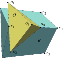
Figure 2. Identity in free space vertex predicate: $r_{0}$ is in the plane of $o_{0}o_{1}o_{2}$.

4. Predicates

An angle polynomial is a polynomial in $t$ that is used in free space construction. We show that every predicate is expressible as the sign of an angle polynomial $f$ evaluated at a zero of an angle polynomial $g$. The only exception is the sign of a contact polynomial $p$ evaluated at a common zero $c$ of contact polynomials $\{p_{1},p_{2},p_{3},p_{4}\}$. We express this form like the other predicates by constructing a polynomial $f$ such that $p(c)=0$ iff $f(t_{0})=0$ as follows.

Let $f$ be the determinant of $\{p_{i},p_{j},p_{k},p\}$, with $\{p_{i},p_{j},p_{k}\}$, $1\leq i<j<k\leq 4$, having a non-zero left 3-by-3 minor at $t=t_{0}$. If $f(t_{0})=0$, $\{p_{i},p_{j},p_{k},p\}$ are linearly dependent in $d$ at $t=t_{0}$, so $p$ is a linear combination of $\{p_{i},p_{j},p_{k}\}$ and $p(c)=0$. If $p(c)=0$, $\{p_{i},p_{j},p_{k},p\}$ must be linearly dependent at $t=t_{0}$ because $p_{i}(c)=p_{j}(c)=p_{k}(c)=0$ and hence $f(t_{0})=0$.

A degenerate predicate has a polynomial $f$ such that $f(t_{0})=0$ for $t=t_{0}$ a zero of $g$. In other words, $f$ and $g$ have a common factor $h$ and $h(t_{0})=0$. This degeneracy is an identity if $h$ results from a common factor of $f$ and $g$ considered as multivariate polynomials in $t$ and in the canonical vertex coordinates. We make such common factor detection fast by enumerating the canonical polynomials, factoring them, and storing the results in a table.

5. Angle polynomials

We represent an angle polynomial with an a-poly: a list of elements of the form $L_{O}-L_{R}$ with $L_{O}$ and $L_{R}$ lists of vertices of $O$ and of $R$ in increasing index order. Elements are in order of increasing $|L_{O}|+|L_{R}|$, then increasing $|L_{O}|$, then increasing vertex index (lexicographically). There are three kinds of a-polys.

The first kind represents the angle polynomials at whose zeros four contacts can occur. It has three types of elements. A 1-contact denotes a contact polynomial. A 2-contact $o_{h}-r_{i}r_{j}$ denotes 1-contacts $o_{h}-r_{i}r_{j}r_{k}$ and $o_{h}-r_{i}r_{j}r_{l}$ that jointly constrain $o_{h}$ to the line $r_{i}r_{j}$; likewise $o_{h}o_{i}-r_{j}$. A 3-contact $o_{h}-r_{i}$ denotes three polynomials whose zeros are the configurations where the two vertices coincide. A list of elements that together denote four polynomials comprises an a-poly.

The second kind represents an angle polynomial that is zero when an edge of one polyhedron and two edges of the other polyhedron are parallel to a common plane. It has three elements of types $o_{i}o_{j}-$ and $-r_{i}r_{j}$, for example $(o_{1}o_{2}-,-r_{1}r_{2},-r_{4}r_{5})$. However, if the two edges share a vertex, we contract $(o_{h}o_{i}-,-r_{j}r_{k},-r_{j}r_{l})$ to $(o_{h}o_{i}-r_{j}r_{k}r_{l})$, corresponding to an edge parallel to a facet. Likewise, $(o_{h}o_{i}o_{j}-r_{k}r_{l})$. The third kind corresponds to the 3-by-3 left minor (Sec. 3): the $d$-coefficients of three contact polynomials. The $d$-coefficients of $o_{i}o_{j}o_{k}-r_{l}$ and $o_{i}-r_{i}r_{j}r_{k}$ do not depend on $r_{l}$ and $o_{i}$, hence the elements are of type $o_{i}o_{j}o_{k}-$, $-r_{i}r_{j}r_{k}$, or $o_{h}o_{i}-r_{j}r_{k}$.

The derivation of the angle polynomials from their a-polys is as follows.

Four 1-contacts

The contact expressions (Table 1) have the form $d\cdot n+k$. The vectors $n$ have the form $a$, $\Theta(t)a$, or $a\times\Theta(t)b$ and the summands of the scalar $k$ have the form $a\cdot b$ or $a\cdot\Theta(t)b$ with $a$ and $b$ constant vectors. The angle polynomial is the numerator of

$$\left|\begin{array}[]{cccc}n_{1x}&n_{1y}&n_{1z}&k_{1}\\ n_{2x}&n_{2y}&n_{2z}&k_{2}\\ n_{3x}&n_{3y}&n_{3z}&k_{3}\\ n_{4x}&n_{4y}&n_{4z}&k_{4}\end{array}\right|.$$

Expanding in terms of minors using the last column, $k_{1}$ has minor $n_{2}\cdot(n_{3}\times n_{4})$. Using the formula, $u\times(v\times w)=(u\cdot w)v-(u\cdot v)w$, each minor reduces to a sum of terms of the form $a\cdot b$, $a\cdot\Theta(t)b$, or $(a\cdot\Theta(t)b)(c\cdot\Theta(t)d)$. Applying equation (1) and clearing the denominator reduces $k_{1}$, $k_{2}$, and $k_{3}$ to quadratics in $t$ and reduces the minors to quartics in $t$, so the angle polynomial has degree 6.

One 2-contact and two 1-contacts

For a 2-contact $o_{i}o_{j}-r_{k}$, $c(r_{k})=d+\Theta(t)r_{k}$ is on the line of $o_{i}o_{j}$, so $d$ is on the line through $o_{i}-\Theta(t)r_{k}$ and $o_{j}-\Theta(t)r_{k}$. We intersect this line with the planes of the other two contact polynomials. We express the line as $\lambda u+v$ with $u=o_{j}-o_{i}$ and $v=o_{j}-\Theta(t)r_{k}$, compute the values $\lambda_{i}=-(n_{i}\cdot v+k_{i})/(n_{i}\cdot u)$ where the line intersects the two planes $n_{i}\cdot p+k_{i}$, set $\lambda_{1}=\lambda_{2}$, and cross multiply to obtain a quartic angle polynomial. Similarly 2-contact $o_{i}-r_{j}r_{k}$ corresponds to a line with $u=\Theta(t)(r_{j}-r_{k})$ and $v=o_{i}-\Theta(t)r_{j}$.

Two 2-contacts

The expression is the signed volume of the four points that define the lines of the 2-contacts, which yields a quartic angle polynomial. Figure 2 illustrates this situation.

One 3-contact and one 1-contact

For a 3-contact $o_{i}-r_{j}$, $o_{i}=d+\Theta(t)r_{j}$. We substitute $d=o_{i}-\Theta(t)r_{j}$ into the 1-contact polynomial to obtain a quadratic angle polynomial.

Other kinds

The second, $(-r_{i_{1}}r_{j_{1}},-r_{i_{2}}r_{j_{2}},o_{i_{3}}o_{j_{3}}-)$ and $(-r_{i_{1}}r_{j_{1}},o_{i_{2}}o_{j_{2}}-,o_{i_{3}}o_{j_{3}}-)$, has expressions that yield quadratic angle polynomials $\Theta(t)((r_{j_{1}}-r_{i_{1}})\times(r_{j_{2}}-r_{i_{2}}))\cdot(o_{j_{3}}-o_{i_{3}})$ and $\Theta(t)(r_{j_{1}}-r_{i_{1}})\cdot((o_{j_{2}}-o_{i_{2}})\times(o_{j_{3}}-o_{i_{3}}))$. The second has expression $(n_{1}\times n_{2})\cdot n_{3}$, where $o_{i}o_{j}o_{k}-$ has normal $n=(o_{j}-o_{i})\times(o_{k}-o_{i})$, $-r_{i}r_{j}r_{k}$ has normal $n=\Theta(t)((r_{j}-r_{i})\times(r_{k}-r_{i}))$, and $o_{h}o_{i}-r_{j}r_{k}$ has normal $n=(o_{i}-o_{h})\times\Theta(t)(r_{k}-r_{j})$. The third has the same polynomials as the quartic minor polynomials above in the four 1-contacts case.

6. Factoring

This section gives an algorithm for factoring angle polynomials represented as a-polys. Two a-polys are equivalent if a vertex bijection maps one to the other. The bijection maps a factorization of one to a factorization of the other. The factoring algorithm uses a table that contains the factorization of a representative a-poly from each equivalence class. Sec. 7 explains how we constructed this table. It is available in the web directory http://www.cs.miami.edu/~vjm/robust/identity.

Identity detection requires that an irreducible polynomial be denoted by a unique a-poly, so one can detect if different a-polys have a common factor. One problem is that nonequivalent a-polys can denote the same polynomial. We solve this problem by selecting the factors in the table from a minimal subset of the equivalence classes that we call basis classes. A second problem is that equivalent a-polys can denote the same polynomial. This problem is so rare that we can record all the basis a-polys that generate a factor, called its factor set, and select a unique one during factoring. The factoring algorithm maps an input a-poly to the representative of its equivalence class, obtains the factor sets of the representative from the table, and applies the inverse map to obtain sets of a-polys in the variables of the input a-poly. To achieve uniqueness, it selects the lexicographical minimum from each set, using a vertex order that we indicate by the $o$ and $r$ indices.

6.1. Mapping an a-poly to its representative

The mapping algorithm generates the permutations of the input a-poly such that the elements remain increasing in $|L_{O}|+|L_{R}|$ then in $|L_{O}|$ (but disregarding the lexicographical order of vertex indices). For each permuted contact list, it assigns each vertex an indicator: a bit string in which a 1 in position $k$ indicates that the vertex appears in the $k$th element. It labels a permutation with its $O$ vertex indicators in decreasing order followed by its $R$ vertex indicators in decreasing order. It selects the permutation with the largest label, replaces the $i$th $O$ vertex in indicator order by the canonical vertex $o_{i}$, and likewise for the $R$ vertices and $r_{i}$. If two vertices have the same indicator, both orders yield the same output because the indices of an a-poly are placed in increasing order.

For example, in a-poly $(o_{27}-r_{22}r_{66}r_{86},o_{43}-r_{22}r_{66}r_{86},o_{27}o_{51}-r_{15}r_{86},o_{27}o_{43}-r_{75}r_{86})$, $o_{27}$ has indicator $1011$, and the indicator list is 1011,0101,0010;1111,1100,1100,0010,0001. The permutations swap the first two and/or last two elements. Swapping the last two yields the maximal indicator list 1011,0110,0001;1111,1100,1100,0010,0001 and the representative $(o_{0}-r_{0}r_{1}r_{2},o_{1}-r_{0}r_{1}r_{2},o_{0}o_{1}-r_{0}r_{3},o_{0}o_{2}-r_{0}r_{4})$. In the table, this representative has factor sets $\{(o_{0}o_{1}-r_{0}r_{1}r_{2})\}$ and $\{(-o_{0}o_{1}o_{2},o_{0}o_{1}-r_{0}r_{3},o_{0}o_{2}-r_{0}r_{4})\}$. The inverse vertex mapping yields the factors $(o_{27}o_{43}-r_{22}r_{66}r_{86})$ and $(-r_{22}r_{66}r_{86},o_{27}o_{43}-r_{75}r_{86},o_{27}o_{51}-r_{15}r_{86})$.

6.2. Uniqueness

Fig. 3 illustrates how a-polys can have the same polynomial. The 1-contacts $o_{0}o_{1}-r_{0}r_{1}$, $o_{0}o_{1}-r_{2}r_{3}$, and $o_{0}o_{1}o_{2}-r_{4}$ determine the angle parameter $t$ because they are invariant under translation parallel to $o_{0}o_{1}$. Translating $R$ parallel to $o_{0}o_{1}$ until one element becomes a 2-contact yields an a-poly $C_{i}$ that is zero at the same $t$ values. If $r_{0}r_{1}$ hits $o_{0}$, $C_{1}=(o_{0}-r_{0}r_{1},o_{0}o_{1}-r_{2}r_{3},o_{0}o_{1}o_{2}-r_{4})$ (Fig. 3b) and if $r_{2}r_{3}$ hits $o_{1}$, $C_{2}=(o_{1}-r_{2}r_{3},o_{0}o_{1}-r_{0}r_{1},o_{0}o_{1}o_{2}-r_{4})$. These a-polys are equivalent under the map from $C_{1}$ to $C_{2}$: $o_{0}\rightarrow o_{1}$, $o_{1}\rightarrow o_{0}$, $o_{2}\rightarrow o_{2}$, $r_{0}\rightarrow r_{2}$, $r_{1}\rightarrow r_{3}$, $r_{2}\rightarrow r_{0}$, $r_{3}\rightarrow r_{1}$, $r_{4}\rightarrow r_{4}$. There are also $C_{3}$ and $C_{4}$ where $r_{0}r_{1}$ hits $o_{1}$ or $r_{2}r_{3}$ hits $o_{0}$ and $C_{5}=(o_{0}o_{2}-r_{4},o_{0}o_{1}-r_{0}r_{1},o_{0}o_{1}-r_{2}r_{3})$ and $C_{6}=(o_{1}o_{2}-r_{4},o_{0}o_{1}-r_{0}r_{1},o_{0}o_{1}-r_{2}r_{3})$ where $r_{4}$ hits $o_{0}o_{2}$ or $o_{1}o_{2}$. $C_{5}$ and $C_{6}$ are not equivalent to $C_{1}$, $C_{2}$, $C_{3}$, and $C_{4}$ because their first element has two $O$ vertices, not one.

(a)	(b)

Figure 3. Equivalent a-polys: (a) translation parallel to $o_{0}o_{1}$ preserves circled contacts $o_{0}o_{1}-r_{0}r_{1}$, $o_{0}o_{1}-r_{2}r_{3}$, and $o_{0}o_{1}o_{2}-r_{4}$; (b) a-poly $(o_{0}-r_{0}r_{1},o_{0}o_{1}-r_{2}r_{3},o_{0}o_{1}o_{2}-r_{4})$.

The a-poly $(o_{1}-r_{0}r_{1}r_{2},o_{0}o_{1}-r_{3}r_{4},o_{0}o_{1}-r_{5}r_{6},o_{o}o_{1}o_{2}-r_{7})$ maps to the representative $(o_{0}-r_{0}r_{1}r_{2},o_{0}o_{1}-r_{3}r_{4},o_{0}o_{1}-r_{5}r_{6},o_{o}o_{1}o_{2}-r_{7})$ with factor sets $\{(o_{0}o_{1}-r_{0}r_{1}r_{2})\}$ and

$$\{(o_{0}-r_{3}r_{4},o_{0}o_{1}-r_{5}r_{6},o_{0}o_{1}o_{2}-r_{7}),(o_{0}-r_{5}r_{6},o_{0}o_{1}-r_{3}r_{4},o_{0}o_{1}o_{2}-r_{7}),$$

$$(o_{1}-r_{3}r_{4},o_{0}o_{1}-r_{5}r_{6},o_{0}o_{1}o_{2}-r_{7}),(o_{1}-r_{5}r_{6},o_{0}o_{1}-r_{3}r_{4},o_{0}o_{1}o_{2}-r_{7})\}$$

because the second factor is equivalent to $C_{1},\ldots,C_{4}$. Its factor set does not contain a-polys equivalent to $C_{5}$ and $C_{6}$ because their class is not in the basis. The inverse map (in this case swapping $o_{0}$ and $o_{1}$) results in factor sets $\{(o_{0}o_{1}-r_{0}r_{1}r_{2})\}$ and

$$\{(o_{1}-r_{3}r_{4},o_{0}o_{1}-r_{5}r_{6},o_{0}o_{1}o_{2}-r_{7}),(o_{1}-r_{5}r_{6},o_{0}o_{1}-r_{3}r_{4},o_{0}o_{1}o_{2}-r_{7}),$$

$$(o_{0}-r_{3}r_{4},o_{0}o_{1}-r_{5}r_{6},o_{0}o_{1}o_{2}-r_{7}),(o_{0}-r_{5}r_{6},o_{0}o_{1}-r_{3}r_{4},o_{0}o_{1}o_{2}-r_{7})\}.$$

The algorithm selects the (minimal) third element $(o_{0}-r_{3}r_{4},o_{0}o_{1}-r_{5}r_{6},o_{0}o_{1}o_{2}-r_{7})$ of the second set as the second factor.

7. Constructing the table of factors

This section explains how we enumerate the a-poly equivalence classes (Sec. 7.1), factor the class representatives and select a basis (Sec. 7.2), and construct the table of factors (Sec. 7.3). The factoring algorithm is probabilistic and depends on the completeness assumption that the factors of a-polys are a-polys. If this assumption were false, the algorithm would have failed. We verify the table to a high degree of certainty using standard techniques for testing polynomial identities (Sec. 7.4).

7.1. Equivalence classes

We enumerate the a-poly classes as follows. Let $a_{i}$, $b_{i}$, $c_{i}$, $d_{i}$, $e_{i}$, and $f_{i}$ denote vertices and define $s_{i}=\{a_{i}-d_{i}\}$, $t_{i}=\{a_{i}-d_{i}e_{i},a_{i}b_{i}-d_{i}\}$, $u_{i}=\{a_{i}-d_{i}e_{i}f_{i},a_{i}b_{i}-d_{i}e_{i},a_{i}b_{i}c_{i}-d_{i}\}$, $v_{i}=\{a_{i}b_{i}-c_{i}d_{i}e_{i},a_{i}b_{i}c_{i}-d_{i}e_{i}\}$, $w_{i}=\{-a_{i}b_{i},a_{i}b_{i}-\}$, $x_{i}=\{-a_{i}b_{i}c_{i},a_{i}b_{i}-c_{i}d_{i},a_{i}b_{i}c_{i}-\}$. We generate the a-polys that are lists of $k$-contacts with the sets $s_{1}\times{}u_{2}$ (a 3-contact and a 1-contact), $t_{1}\times{}t_{2}$ (two 2-contacts), $t_{1}\times{}u_{2}\times{}u_{3}$ (a 2-contact and two 1-contacts), and $u_{1}\times{}u_{2}\times{}u_{3}\times{}u_{4}$ (four 1-contacts). We generate the other kinds of a-polys with the sets $v_{1}$ (edge parallel to facet), $w_{1}\times{}w_{2}\times{}w_{3}$ (edges parallel to plane), and $x_{1}\times{}x_{2}\times{}x_{3}$ (3-by-3 left minor). For each element of each set, we assign $O$ vertices to the $a_{i},b_{i},c_{i}$ in every possible manner. Starting from $o_{0}$, we assign increasing indices to the vertices of an edge or a facet. We assign $R$ vertices to $d_{i},e_{i},f_{i}$ likewise. The highest index is 11.

For example, $s_{1}\times{}u_{2}=\{(a_{1}-d_{1},a_{2}-d_{2}e_{2}f_{2}),(a_{1}-d_{1},a_{2}b_{2}-d_{2}e_{2}),(a_{1}-d_{1},a_{2}b_{2}c_{2}-d_{2})\}$. We must set $a_{1}=o_{0}$. We can set $a_{2}=o_{0}$ or $a_{2}=o_{1}$ because $a_{2}$ is in a different feature, and then assign increasing indices to $b_{2}$ and $c_{2}$. Similarly for $d_{1}$, $d_{2}$, $e_{2}$, and $f_{2}$. The results are
$\{(o_{0}-r_{0},o_{0}-r_{0}r_{1}r_{2}),(o_{0}-r_{0},o_{1}-r_{0}r_{1}r_{2}),(o_{0}-r_{0},o_{0}-r_{1}r_{2}r_{3}),(o_{0}-r_{0},o_{1}-r_{1}r_{2}r_{3}),$
  $(o_{0}-r_{0},o_{0}o_{1}-r_{0}r_{1}),(o_{0}-r_{0},o_{1}o_{2}-r_{0}r_{1}),(o_{0}-r_{0},o_{0}o_{1}-r_{1}r_{2}),(o_{0}-r_{0},o_{1}o_{2}-r_{1}r_{2}),$
  $(o_{0}-r_{0},o_{0}o_{1}o_{2}-r_{0}),(o_{0}-r_{0},o_{1}o_{2}o_{3}-r_{0}),(o_{0}-r_{0},o_{0}o_{1}o_{2}-r_{1}),(o_{0}-r_{0},o_{1}o_{2}o_{3}-r_{1})\}$.

The enumeration yields about one million a-polys. Generating their representatives (Sec. 6) and removing duplicates yields 30,564 equivalence class representatives.

7.2. Basis classes

We factor the representatives probabilistically. We replace the canonical coordinates of $o_{0},\ldots,o_{11}$ and $r_{0},\ldots,r_{11}$ with random integers, construct the resulting univariate integer polynomials, and factor them with Mathematica. An irreducible univariate implies that the canonical polynomial is irreducible; the converse is true with high probability.

An a-poly depends on a vertex if its univariate changes when the coordinates of the vertex are assigned different random integers. For example, $(o_{0}o_{1}-r_{0},o_{2}-r_{1}r_{2}r_{3},o_{2}-r_{1}r_{2}r_{4})$ does not depend on $r_{3}$ and $r_{4}$ because $o_{2}-r_{1}r_{2}r_{3}$ and $o_{2}-r_{1}r_{2}r_{4}$ can be replaced by $o_{2}-r_{1}r_{2}$: $o_{2}$ in contact with $r_{1}r_{2}r_{3}$ and $r_{1}r_{2}r_{4}$ is equivalent to $o_{2}$ in contact with $r_{1}r_{2}$. An a-poly is complete if it depends on all of its vertices. An angle polynomial is contiguous if it depends on $o_{0},o_{1},\ldots,o_{l}$ and $r_{0},r_{1},\ldots,r_{m}$ for some $l$ and $m$. A complete representative is also contiguous because we assign vertices to the indicators contiguously (Sec. 6).

We select a basis of complete, contiguous, and irreducible a-polys, represented by the representatives of their classes. (We prove that such a basis exists by verifying the table of factors (Sec. 7.4).) We construct a map $I$ from the univariate of each basis a-poly to the set of basis a-polys that generate it. In the Sec. 6.2 example, $C_{1}$ is in the basis and generates a univariate $p$. The equivalent a-polys $C_{2}$, $C_{3}$, and $C_{4}$ also generate $p$, so $I(p)=\{C_{1},C_{2},C_{3},C_{4}\}$. Although $C_{5}$ and $C_{6}$ also generate $p$, they are not in $I(p)$ because they belong to another (necessarily non-basis) equivalence class.

The algorithm visits each representative $\rho$. If $\rho$ is complete and its univariate $p$ is irreducible but $I(p)=\emptyset$, the algorithm adds $\rho$ to the basis representatives, permutes its vertices in every way, calculates the univariate $u$ for each resulting a-poly $a$, and adds $a$ to the set $I(u)$.

The condition $I(p)=\emptyset$ prevents adding an a-poly to the basis whose univariate is already generated by a member of a basis class. For example, $\rho_{1}=(-r_{0}r_{1}r_{2},-r_{0}r_{3}r_{4},o_{0}o_{1}-r_{0}r_{5})$ is assigned to the basis. Later, $\rho_{2}=(o_{0}-r_{0}r_{1},o_{0}-r_{2}r_{3}r_{4},o_{0}o_{1}-r_{2}r_{5})$ is complete and has an irreducible univariate that is generated by $(-r_{0}r_{1}r_{2},-r_{2}r_{3}r_{4},o_{0}o_{1}-r_{2}r_{5})$, which is a permutation of $\rho_{1}$. Since every permutation of $\rho_{1}$ is in $I$, $\rho_{2}$ is not assigned to the basis.

7.3. Factor table

The factor table provides a list of factor sets for each representative. For a basis representative $\rho$ with univariate $p$, the list is $\langle I(p)\rangle$. If $\rho$ is not in the basis, we process each factor $f$ of $p$ as follows.

1) Determine which vertices $f$ depends on. Randomly change a vertex of $\rho$, generate the new univariate, and factor it. If $f$ is not a factor, it depends on the vertex.

2) Rename the vertices of $\rho$ to obtain a $\rho^{\prime}$ for which the factor $f^{\prime}$ that corresponds to $f$ is contiguous. Let $f$ depend on $o_{i_{0}},o_{i_{1}},\ldots,o_{i_{m^{\prime}}}$ and $r_{j_{0}},r_{j_{1}},\ldots,r_{j_{n^{\prime}}}$ but not on $o_{i_{m^{\prime}+1}},o_{i_{m^{\prime}+2}},\ldots,o_{i_{m}}$ and $r_{j_{n^{\prime}+1}},r_{j_{n^{\prime}+2}},\ldots,r_{j_{n}}$. Substitute $o_{i_{k}}\rightarrow o_{k}$ for $k=1,\ldots,m$ and $r_{i_{k}}\rightarrow r_{k}$ for $k=1,\ldots,n$.

3) Find the factor $f^{\prime}$ of $\rho^{\prime}$ that depends on $o_{0},\ldots,o_{m^{\prime}}$ and $r_{0},\ldots,r_{n^{\prime}}$, and has the same degree as $f$. (This factor is unique; otherwise, we would consider every match.)

4) Look up $I(f^{\prime})$ and invert the vertex substitution to obtain a factor set.

For example, the univariate of $\rho=(o_{0}o_{1}-r_{0}r_{1},o_{2}o_{3}o_{4}-r_{2},o_{2}o_{3}o_{4}-r_{3},o_{5}o_{6}o_{7}-r_{4})$ has a factor $f$ that depends on all its variables and a quadratic factor $g$ that depends on $o_{2},o_{3},o_{4},r_{2},r_{3}$. The factor set of $f$ is $I(f)=\{(o_{2}o_{3}o_{4}-,o_{5}o_{6}o_{7}-,o_{0}o_{1}-r_{0}r_{1})\}$. To obtain the factor set of $g$, substitute ${o_{2},o_{3},o_{4},o_{0},o_{1},r_{2},r_{3},r_{0},r_{1}}\rightarrow{o_{0},o_{1},o_{2},o_{3},o_{4},r_{0},r_{1},r_{2},r_{3}}$. The quadratic factor $g^{\prime}$ of $\rho^{\prime}=(o_{3}o_{4}-r_{2}r_{3},o_{0}o_{1}o_{2}-r_{0},o_{0}o_{1}o_{2}-r_{1},o_{5}o_{6}o_{7}-r_{4})$ depends on $o_{0}o_{1}o_{2}$ and $r_{0}r_{1}$, and $I(g^{\prime})=\{(o_{0}o_{1}o_{2}-r_{0}r_{1})\}$. Inverting the vertex substitution yields the second factor set of $\rho$: $\{(o_{2}o_{3}o_{4}-r_{2}r_{3})\}$.

To save space, we do not add entries to $I$ corresponding to permutations of basis representatives with degree-6 univariates because they cannot be proper factors. To test if $\rho$ with irreducible degree-6 univariate $p$ is in the basis, we generate the permutations of $\rho$ and their univariates. If none has an entry in $I$, $\rho$ is in the basis, and we add an entry for $p$ to $I$. If the univariate $p^{\prime}$ of a permutation has an entry in $I$, the sole factor set of $\rho$ is the result of applying the inverse of the permutation to $I(p^{\prime})$.

7.4. Analysis

Out of 30,564 representatives, 15,306 are basis, 991 are constant, 3840 are irreducible but non-basis, 8263 have two factors (including 260 squares), and 2164 have three factors (including 6 cubes). Since a predicate is an a-poly evaluated on a zero of a basis polynomial, we listed $450,000,000\approx 30,564\cdot 15,306$ predicates in the introduction. Likewise, we stated the number of identities as $13,000\approx 1\cdot 3840+2\cdot 8263+3\cdot 2164$ ways of evaluating a non-basis polynomial on the zero of a factor. Of the irreducible representative polynomials, 363 have two basis a-polys, 50 have three, 194 have four, and 194 have six.

Each factorization $f_{1}f_{2}\cdots f_{m}|f$ is equivalent to a polynomial identity $f-af_{1}f_{2}\cdots f_{m}=0$ for some constant $a$. Instead of analyzing the probability of failure of the algorithm, we verify the identities probabilistically using Schwartz’s lemma [9]. We use random 20-bit values modulo a prime $p$. The first substitution determines $a$ and the rest verify the identity. Verifying all 15,258 factorizations once takes 2 seconds and 10 minutes of verification reduces the probability of an error to below $10^{-1000}$. This also constitutes a probabilistic proof of the completeness assumption.

The running time for factor table construction was one CPU day. All but one CPU hour was spent generating the permutations of the degree-six irreducible polynomials to test if they are in the basis. The worst case is four contacts between $O$ vertices and $R$ facets or vice versa, which have about 70 billion permutations. The tests all succeeded, so perhaps we could have avoided this cost by proving a theorem.

8. Contact set subdivision

We continue our discussion of free space with an algorithm for constructing the faces of its boundary. The contact set of a vertex/facet or edge/edge pair is the set of configurations where the two features are in contact. We construct the subdivision of a contact set induced by the other contact sets. Each predicate used in the construction has the same zero set as an a-poly, so identity detection applies. The remaining (and substantial) step in free space construction is to stitch the faces into a boundary representation of the free cells.

Contact sets

The contact set for a triangle $o_{h}o_{i}o_{j}$ of $O$ and a vertex $r_{k}$ of $R$ is the set of configurations $c=(t,d)$ such that $c(r_{k})=d+\Theta(t)r_{k}$ lies on $o_{h}o_{i}o_{j}$. Hence, $d$ lies on the triangle $o_{h}-\Theta(t)r_{k},o_{i}-\Theta(t)r_{k},o_{j}-\Theta(t)r_{k}$. This triangle is a cross-section of the contact set whose vertices are rational functions of $t$. Similarly, the contact set for $o_{h}$ and $r_{i}r_{j}r_{k}$ is the parameterized triangle $o_{h}-\Theta(t)r_{i},o_{h}-\Theta(t)r_{j},o_{h}-\Theta(t)r_{k}$, and the contact set for $o_{h}o_{i}$ and $r_{j}r_{k}$, is the parameterized parallelogram $o_{h}-\Theta(t)r_{j},o_{h}-\Theta(t)r_{k},o_{i}-\Theta(t)r_{j},o_{i}-\Theta(t)r_{k}$.

Contact facets

We are only interested in the portion of a contact set that is on the boundary of the free space. A necessary condition is that the interiors of $O$ and $c(R)$ are disjoint in a neighborhood of their point of contact. A contact facet is the restriction of a contact set to the intervals of $t$ values where this condition holds. We express the condition in terms of the signs of a-polys (ignoring the vertex index order rule), hence the intervals are bounded by zeros of a-polys. For $o_{h}o_{i}o_{j}$ and $r_{k}$, $(o_{h}o_{i}o_{j}-r_{k}r_{l})$ must be positive for every edge $r_{k}r_{l}$; likewise for $o_{h}$ and $r_{i}r_{j}r_{k}$. For $o_{h}o_{i}$ and $r_{j}r_{k}$, let $o_{h}o_{i}$ be incident on the triangles $o_{h}o_{i}m_{1}$ and $o_{i}o_{h}m_{2}$, let $r_{j}r_{k}$ be incident on the triangles $r_{j}r_{k}n_{1}$ and $r_{k}r_{j}n_{2}$, and let $s_{x}$ and $t_{x}$ be the signs of $(o_{h}o_{i}m_{x}-r_{j}r_{k})$ and $(o_{h}o_{i}-r_{j}r_{k}n_{x})$ for $x=1,2$. The interiors are locally disjoint if $s_{1}=s_{2}=-t_{1}=-t_{2}$.

The parameterized edges of a contact facet are called contact facet edges and are in the zero sets of 2-contacts. The parameterized vertices are called contact facet vertices and are in the zero sets of 3-contacts.

Contact facet subdivision

At a fixed $t$, each contact facet (triangle or parallelogram) is intersected and subdivided by other contact facets. The intersection of two facets is called an FF-edge, and the intersection of a facet edge and a facet is called an EF-vertex. The endpoints of an FF-edges are facet vertices or EF-vertices. Two FF-edges intersect at an FFF-vertex, the intersection of three facets.

Structure changes

The subdivision of a contact facet by other contact facets is continuous in $t$, except for four types of structure changes. I. Facets appear or disappear at the bounds of their intervals. II. FF-edges appear or disappear when a facet vertex hits a facet or when two facet edges intersect. In Fig. 4, the FF-edge $vw$ appears when the facet vertex $a$ hits the facet $def$ or when the facet edges $ac$ and $de$ intersect. III. FFF-vertices appear or disappear when a facet edge $e$ hits an FF-edge, and two EF-vertices swap position on $e$. In Fig. 5, the EF-vertices $j$ and $k$ swap on the facet edge $df$ when it hits the FF-edge $gi$, and the FFF-vertex $x$ appears. IV. The FFF-vertices of four facets swap position along their FF-edges when the facets intersect at a vertex. In Fig. 6, three facets intersect $abcd$ in FF-edges $ps$, $qt$, and $ur$, FFF-vertices $i$ and $j$ swap on $ur$, $j$ and $k$ swap on $qt$, and $i$ and $k$ swap on $ps$.

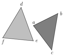
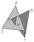
(a)
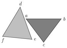
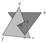
(b)

Figure 4. Type II structure changes: (a) vertex–facet, (b) edge–edge.

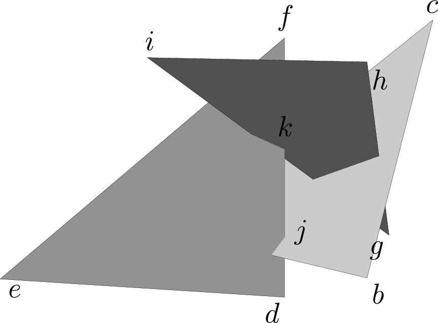
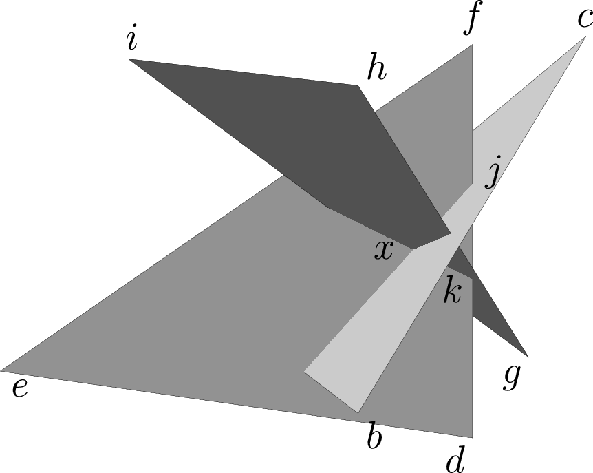
Figure 5. Type III structure change.

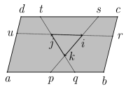
Figure 6. Type IV structure change.

Structure change a-polys

Structure changes occur at zeros of a-polys. The Type I facet interval a-polys are discussed above. Fig. 7 describes the a-polys of the other types.

IIa	a) zero distance from a facet vertex to the plane of a facet.
	b) 3-contact of vertex, 1-contact of facet.
IIb	a) zero volume of the tetrahedron defined by two facet edges.
	b) 2-contact of each edge.
III	a) zero distance from an EF-vertex to the plane of a facet.
	b) 2-contact of EF-vertex edge, 1-contact of EF-vertex facet, 1-contact of facet.
IV	a) zero distance between two FFF-vertices along an FF-edge.
	b) 1-contact of each facet (four in all) incident on the FFF-vertices.

Figure 7. Structure change conditions (a) and a-polys (b).

Sweep algorithm

We construct the subdivision of a contact set by constructing the subdivision of each contact facet at its initial $t$ value, sweeping along its $t$ interval, computing the $t$ values where the subdivision undergoes structure changes, and updating the structure. The sweep state is the ordered list of EF-vertices along each contact edge, the set of interior EF-vertices, the set of FF-edges, and the ordered list of FFF-vertices along each FF-edge. The sweep events are the angles where 1) EF-vertices and 2) FF-edges appear or disappear (at a Type I or II structure change) 3) an internal EF-vertex hits an FF-edge (III), 4) two EF-vertices swap on a contact edge (III), or 5) two FFF vertices swap on an FF-edge (IV). FFF-vertices can appear and disappear at events 2, 3 or 4. Events 1 and 2 are calculated before the sweep, event 3 is calculated at a 1 or 2 event, and events 4 and 5 are calculated when two vertices become adjacent on an edge. To calculate event 3, compute the zeros of its a-poly (Fig. 7III). When sweeping through each zero, check if the FF-edge and EF-vertex exist at that angle and evaluate predicates at that angle to determine if the EF-vertex hits the line of the FF-edge between its current endpoints, and if so, where in the list of FFF-vertices the new one should be inserted. Similarly for 4 and 5.

Handling identities

Each predicate has the same zero set as an a-poly. For example, testing if a contact edge pierces a contact facet involves testing an (endpoint) contact vertex vs. the contact facet. The associated a-poly contains the vertex 3-contact and the facet 1-contact. Before evaluating a predicate at an event angle, we check for identity. An identity results from evaluating the predicate at a parameter $t$ that is a zero of a $k\geq 1$ repeated irreducible factor of the a-poly of the predicate. We replace the sign of the predicate with the sign of its $k$th derivative, evaluated using automatic differentiation. The derivative gives the sign of the predicate value immediately after the event, as required by the sweep algorithm.

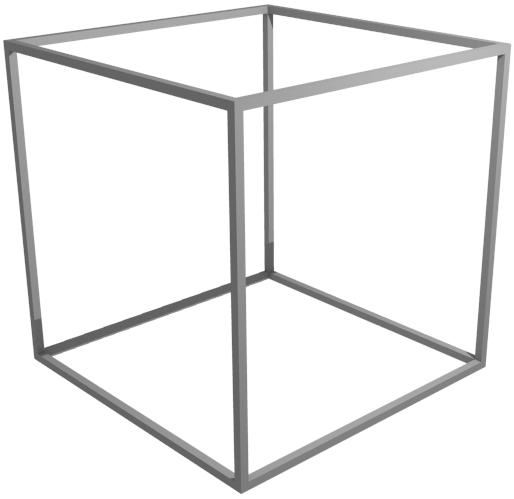
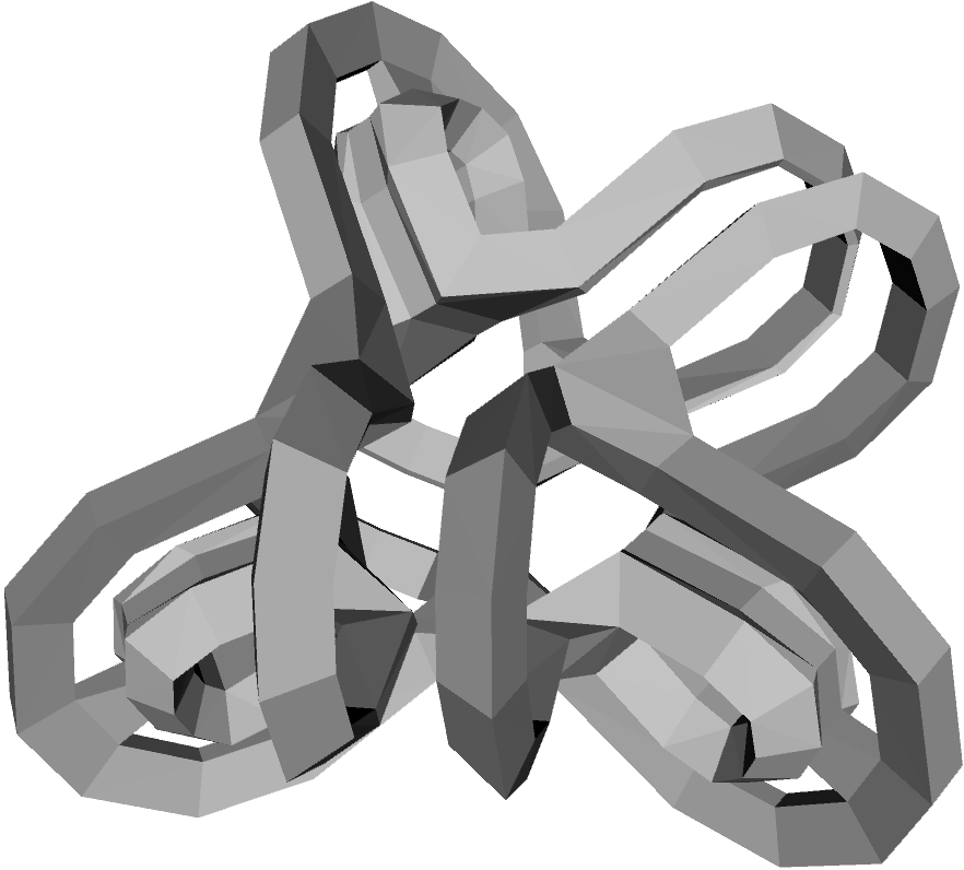
frame: 40 vertices and 96 facets	knot: 480 vertices and 992 facets
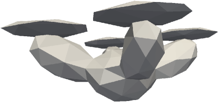
simple: 18 vertices and 32 facets	drone: 189 vertices and 374 facets

Figure 8. Sweep Inputs. Actual frame and knot are large enough for simple and drone to fly through.

9. Results

We measure the running time of predicate evaluation using the factoring algorithm (Sec. 6) for identity detection and compare it to using the greatest common divisor (GCD) for degeneracy detection.

We compute the GCD with Euclid’s algorithm. The main step is polynomial division. We compute the degree of a remainder by finding its nonzero coefficient of highest degree. If the sign of a coefficient is ambiguous in double precision interval arithmetic, we evaluate modulo several 32-bit primes and invoke the Chinese Remainder Theorem (CRT). The a-polys have degree at most 9 in the input coordinates (Sec. 5). The leading coefficient is at most degree 9 in the polynomial coefficients. Hence, CRT requires $\lceil{9\cdot 9\cdot 53/32}\rceil=135$ modulo evaluations. If they are all zero, the coefficient is zero. This analysis assumes that all inputs have the same exponent field and can be replaced by their 53-bit integer mantissas.

In our first set of tests, we selected 100,000 representatives at random and instantiated them on a pool of 12 $O$ vertices and 12 $R$ vertices with random coordinates in $(-1,1)$. We factored the univariates of these a-polys, isolated the zeros of the factors, and stored them in a red-black tree.

Let $t_{h}$ be the $i$th largest real zero of $h$, a factor of a random a-poly $g$. When inserting $t_{h}$ into the tree, it must be compared to prior zeros, such as the $j$th zero $t_{e}$ of $e$, a factor of $f$. If $e=h$ and $i=j$, then $t_{h}=t_{e}$. To measure the running time of the identity detection algorithm (Sec. 6), we add an unnecessary test if $g(t_{e})$ is an identity. This ensures identity tests on random polynomials with both possible answers. Adding these 9,660,759 identity tests (221,252 positive) increases the running time from 6.6 seconds to 18.1 seconds, giving an average identity detection time of 1.2 microseconds.

To test the GCD approach, we drop factoring and the equality test, and replace each polynomial $f$ with its square-free form $f/{\mathrm{GCD}}(f,f^{\prime})$. If the comparison of zeros $t_{f}$ of $f$ and $t_{g}$ of $g$ is ambiguous in double precision, we run the following degeneracy test on $g(t_{f})$. Set $h\leftarrow{\mathrm{GCD}}(f,g)$ and $e=f/h$. If $e(t_{f})$ is unambiguously nonzero, $g(t_{f})$ must be zero. If $e(t_{f})$ and $g(t_{f})$ are both ambiguous, redo these steps with more precision. The additional time was 376 seconds for 81264 degeneracy tests, for an average time of 4627 microseconds. To be sure that $t_{f}=t_{g}$ and not some other zero of $g$, we must check that its comparison with other zeros is unambiguous, so the true cost of the GCD method is even higher.

In the second set of tests, we ran a sweep algorithm (Sec. 8) on the polyhedra shown in Fig. 8. Table 2 shows the average running times for sweeping a facet using factor-based identity detection and GCD degeneracy detection. We sweep either all the facets (tests 1-3) or a large random sample over all angles (test 4).

Table 2. Sweep algorithm: $f$ total number of contact facets, $t_{\mathrm{fac}}$ and $t_{\mathrm{GCD}}$ average running time in seconds for sweeping a facet with our identity detection and GCD-based degeneracy detection.

	$O$	$R$	$f$	$t_{\mathrm{fac}}$	$t_{\mathrm{GCD}}$	$t_{\mathrm{GCD}}/t_{\mathrm{fac}}$
1	frame	simple	2196	0.021	0.533	25.33
2	frame	drone	18812	0.148	2.093	14.13
3	knot	simple	23419	0.023	0.651	27.24
4	knot	drone	235789	0.037	0.857	23.26

The first tests indicate that factor-based identity detection is 3500 times faster than GCD-based degeneracy detection. The sweep tests show that the effect of this improvement entails a factor of 14 speedup in sweep time. Since identity detection is sped up by 3500, factor-based identity detection uses less that 0.5% of the overall running time, versus 90% for GCD-based degeneracy detection.

10. Discussion

We have shown that looking up the factors of an a-poly is much faster than polynomial algebra for zero detection. As an additional advantage, factorization provides a unique representation of each algebraic number as the $i$th zero of an irreducible polynomial.

In future work, we will extend the sweep algorithm to completely construct the subdivision of a contact set. We are missing the surfaces that bound the cells and their nesting order. We will construct a connected component of the free space boundary by visiting the neighboring contact facets, computing their subdivisions, and so on. All the predicates are angle polynomials evaluated at zeros of angle polynomials.

For efficient free space boundary construction, we must eliminate irrelevant contact facets from consideration and must eliminate irrelevant sweep angles for relevant contact facets. One strategy is to construct a polyhedral inner and outer approximation of $R$ as it sweeps through a small angle. For that angle range, the boundary of the rotational free space lies between the boundaries of the translational free spaces of the approximations. We can use our fast polyhedral Minkowski sum software [4] to generate approximations of the rotational free space boundary for a set of angle intervals covering the unit circle. We see no reason that sweeping a relevant facet should have fewer identities than sweeping an irrelevant facet, and so fast identity detection should provide the same speedup as observed in Sec. 9.

We conclude that our identity detection algorithm is useful for the drone–warehouse problem. But does the technique generalize to other domains? We discuss three challenges.

Factor table construction (Sec. 7) depends on the property that the set of polynomials is closed under factorization. What if this is not true for some alternate class of polynomials? We would realize that something was missing when factor table construction failed due to unmatched univariates. We would then analyze the failure to uncover the missing polynomials. (This is how we discovered the three-edge parallel-feature a-polys.) The new polynomials might also have had unmatched factors. However, the process of adding missing factor polynomials must converge because factoring reduces degree.

Representative generation (Sec. 6) depends strongly on the a-poly representation. However, the approach should generalize. A predicate has symmetries on its inputs that leave it alone or flip its sign. Two invocations of a predicate function (with repeated inputs) are isomorphic if one can get from one to the other by applying those symmetries and reindexing inputs. A representative is the isomorphism class member that is lexicographically minimal.

Generalizing the matching of factors to prior classes for table generation would greatly increase the running time because it uses enumeration of permutations. In free space construction for $R$ with $d$ degrees of freedom, the computational complexity is $(3d!)d^{2}$, which would balloon to 80,000 years for $d=6$ (unconstrained rotation and translation). We could use the “Birthday paradox” to match two polynomials by generating the square root of the number of permutations for each one and finding a collision, reducing the running time by a factor of $\sqrt{3d!}$ to less than a day. Moreover, these enumerations can be tested in parallel.

Greater complexity might also increase the time required to construct a representative (Sec. 6) for identity detection, but this cost can be reduced by using a subset of the symmetry group and increasing the size of the lookup table. For example, if we did not reorder the elements, the table size would be 134,082, and if we did not reorder the left and right columns either, it would be 972,806. These tables are easy to generate from the minimal table, and both are reasonable for current RAM sizes.

References

- [1] Cgal, Computational Geometry Algorithms Library. http://www.cgal.org.
- [2] Peter Hachenberger. Exact Minkowski sums of polyhedra and exact and efficient decomposition of polyhedra into convex pieces. Algorithmica, 55:329–345, 2009.
- [3] Dan Halperin. Controlled perturbation for certified geometric computing with fixed-precision arithmetic. In ICMS, pages 92–95, 2010.
- [4] Min-Ho Kyung, Elisha Sacks, and Victor Milenkovic. Robust polyhedral Minkowski sums with GPU implementation. Computer-Aided Design, 67–68:48–57, 2015.
- [5] Naama Mayer, Efi Fogel, and Dan Halperin. Fast and robust retrieval of Minkowski sums of rotating convex polyhedra in 3-space. Computer-Aided Design, 43(10):1258–1269, 2011.
- [6] Victor Milenkovic, Elisha Sacks, and Steven Trac. Robust free space computation for curved planar bodies. IEEE Transactions on Automation Science and Engineering, 10(4):875–883, 2013.
- [7] Elisha Sacks, Nabeel Butt, and Victor Milenkovic. Robust free space construction for a polyhedron with planar motion. Computer-Aided Design, 90C:18–26, 2017.
- [8] Elisha Sacks and Victor Milenkovic. Robust cascading of operations on polyhedra. Computer-Aided Design, 46:216–220, January 2014.
- [9] J. T. Schwartz. Fast probabilistic algorithms for verification of polynomial identities. Journal of the ACM, 27(4):701–717, 1980.