TBD: Benchmarking and Analyzing Deep Neural Network Training

Abstract

The recent popularity of deep neural networks (DNNs) has generated a lot of research interest in performing DNN-related computation efficiently. However, the primary focus is usually very narrow and limited to (i) inference – i.e. how to efficiently execute already trained models and (ii) image classification networks as the primary benchmark for evaluation.

Our primary goal in this work is to break this myopic view by (i) proposing a new benchmark for DNN training, called TBD, that uses a representative set of DNN models that cover a wide range of machine learning applications: image classification, machine translation, speech recognition, object detection, adversarial networks, reinforcement learning, and (ii) by performing an extensive performance analysis of training these different applications on three major deep learning frameworks (TensorFlow, MXNet, CNTK) across different hardware configurations (single-GPU, multi-GPU, and multi-machine). TBD currently covers six major application domains and eight different state-of-the-art models. We present a new toolchain for performance analysis for these models that combines the targeted usage of existing performance analysis tools, careful selection of new and existing metrics and methodologies to analyze the results, and utilization of domain specific characteristics of DNN training. We also build a new set of tools for memory profiling in all three major frameworks; much needed tools that can finally shed some light on precisely how much memory is consumed by different data structures (weights, activations, gradients, workspace) in DNN training. By using our tools and methodologies, we make several important observations and recommendations on where the future research and optimization of DNN training should be focused.

1 Introduction

The availability of large datasets and powerful computing resources has enabled a new type of artificial neural networks—deep neural networks (DNNs [55, 19])—to solve hard problems such as image classification, machine translation, and speech processing [63, 52, 15, 54, 98, 94]. While this recent success of DNN-based learning algorithms has naturally attracted a lot of attention, the primary focus of researchers especially in the systems and computer architecture communities is usually on inference—i.e. how to efficiently execute already trained models, and image classification (which is used as the primary benchmark to evaluate DNN computation efficiency).

While inference is arguably an important problem, we observe that efficiently training new models is becoming equally important as machine learning is applied to an ever growing number of domains, e.g., speech recognition [15, 100], machine translation [18, 69, 91], automobile industry [21, 57], and recommendation systems [34, 53]. But researchers currently lack comprehensive benchmarks and profiling tools for DNN training. In this paper, we present a new benchmark for DNN training, called TBD, that uses a representative set of DNN models covering a broad range of machine learning applications: image classification, machine translation, speech recognition, adversarial networks, reinforcement learning. TBD also incorporates an analysis toolchain for performing detailed resource and performance profiling of these models, including the first publicly available tool for profiling memory usage on major DNN frameworks. Using TBD we perform a detailed performance analysis on how these different applications behave on three DNN training frameworks (TensorFlow [10], MXNet [24], CNTK [102]) across different hardware configurations (single-GPU, multi-GPU, and multi-machine) gaining some interesting insights.

	Image Classification Only	Broader (include non-CNN workloads)
Training	[29][35][37][56][61][62][83][90][95]	[10][22][58][66][75][77][99]
Inference	[12][13][14][25][28][37][39][42][61] [67][68][74][81][86][87][88][90] [103][104]	[10][38][46][51][60][75]

Table 1: The table above shows a categorization of major computer architecture and systems conference papers (SOSP, OSDI, NSDI, MICRO, ISCA, HPCA, ASPLOS) since 2014. These papers are grouped by their focus along two dimensions: Training versus Inference and Algorithmic Breadth. There are more papers which optimize inference over training (25 vs. 16, 4 papers aim for both training and inference). Similarly more papers use image classification as the only application for evaluation (26 vs. 11).

TBD’s benchmark suite and analysis toolchain is driven by the motivation to address three main challenges:

1. Training differs significantly from inference. The algorithmic differences between training and inference lead to many differences in requirements for the underlying systems and hardware architecture. First, backward pass and weight updates, operations unique to training, need to save/stash a large number of intermediate results in GPU memory, e.g., outputs of the inner layers called feature maps or activations [83]. This puts significant pressure on the memory subsystem of modern DNN accelerators (usually GPUs) – in some cases the model might need tens of gigabytes of main memory [83]. In contrast, the memory footprint of inference is significantly smaller, in the order of tens of megabytes [47], and the major memory consumers are model weights rather than feature maps. Second, training usually proceeds in waves of mini-batches, a set of inputs grouped and processed in parallel [43, 101]. Mini-batching helps in avoiding both overfitting and under utilization of GPU’s compute parallelism. Thus, throughput is the primary performance metric of concern in training. Compared to training, inference is computationally less taxing and is latency sensitive.

2. Workload diversity. Deep learning has achieved state-of-the-art results in a very broad range of application domains. Yet most existing evaluations of DNN performance remain narrowly focused on just image classification as their benchmark application, and convolutional neural networks (CNNs) remain the most widely-used models for systems/architecture researchers (Table 1). As a result, many important non-CNN models have not received much attention, with only a handful of papers evaluating non-CNNs such as recurrent neural networks [10, 60, 51]. Papers that cover unsupervised learning or deep reinforcement learning are extremely rare. The computational characteristics of image classification models are very different from these networks, thus motivating a need for a broader benchmark suite for DNN training. Furthermore, given the rapid pace of innovation across the realms of algorithms, systems, and hardware related to deep learning, such benchmarks risk being quickly obsolete if they don’t change with time.

3. Identifying bottlenecks. It is not obvious which hardware resource is the critical bottleneck that typically limits training throughput, as there are multiple plausible candidates. Typical convolutional neural networks (CNNs) are usually computationally intensive, making computation one of the primary bottlenecks in single GPU training. Efficiently using modern GPUs (or other hardware accelerators) requires training with large mini-batch sizes. Unfortunately, as we will show later in Section 4.2, for some workloads (e.g., RNNs, LSTMs) this requirement can not be satisfied due to capacity limitations of GPU main memory (usually 8–16GBs). Training DNNs in a distributed environment with multiple GPUs and multiple machines, brings with it yet another group of potential bottlenecks, network and interconnect bandwidths, as training requires fast communication between many CPUs and GPUs (see Section 4.5). Even for a specific model, implementation and hardware setup pinpointing whether performance is bounded by computation, memory, or communication is not easy due to limitations of existing profiling tools. Commonly used tools (e.g., vTune [80], nvprof [9], etc.) have no domain-specific knowledge about the algorithm logic, can only capture some low-level information within their own scopes, and usually cannot perform analysis on full application executions with huge working set sizes. Furthermore, no tools for memory profiling are currently available for any of the major DNN frameworks.

Our paper makes the following contributions.

• TBD, a new benchmark suite. We create a new benchmark suite for DNN training that currently covers six major application domains and eight different state-of-the-art models. The applications in this suite are selected based on extensive conversations with ML developers and users from both industry and academia. For all application domains we select recent models capable of delivering state-of-the-art results. We will open-source our benchmarks suite later this year and intend to continually expand it with new applications and models based on feedback and support from the community.

• Tools to enable end-to-end performance analysis. We develop a toolchain for end-to-end analysis of DNN training. To perform such analysis, we perform piecewise profiling by targeting specific parts of training using existing performance analysis tools, and then merge and analyze them using domain-specific knowledge of DNN training. As part of the toolchain we also built new memory profiling tools for the three major DNN frameworks we considered: TensorFlow [10], MXNet [24], and CNTK [102]. Our memory profilers can pinpoint how much memory is consumed by different data structures during training (weights, activations, gradients, workspace etc.), thus enabling developer to make easy data-driven decisions for memory optimizations.

• Findings and Recommendations. Using our benchmark suite and analysis tools, we make several important observations and recommendations on where the future research and optimization of DNNs should be focused. We include a few examples here: (1) We find that the training of state-of-the-art RNN models is not as efficient as for image classification models, because GPU utilization for RNN models is 2–3$\times$ lower than for most other benchmark models. (2) We find that GPU memory is often not utilized efficiently, the strategy of exhausting GPU memory capacity with large mini-batch provides limited benefits for a wide range of models. (3) We also find that the feature maps, the output of the DNN intermediate layers, consume 70–90% of the total memory footprint for all our benchmark models. This is a significant contrast to inference, where footprint is dominated by the weights. These observations suggest several interesting research directions, including efficient RNN layer implementations and memory footprint reduction optimizations with the focus on feature maps.

The TBD benchmark suite and the accompanying measurement toolchain, and insights derived from them will aid researchers and practitioners in computer systems, computer architecture, and machine learning to determine where to target their optimizations efforts within each level in the DNN training stack: (i) applications and their corresponding models, (ii) currently used libraries (e.g., cuDNN), and (iii) hardware that is used to train these models. We also hope that our paper will instigate additional follow-up work within the Sigmetrics community aimed at providing DNN research with a more rigorous foundation rooted in measurements and benchmarking.

In the rest of this paper, we first provide some background on DNN training, both single-GPU and distributed training (with multiple GPUs and multiple machines) in Section 2. We then present our methodology, explaining which DNN models we selected to be included in our benchmark suite and why, and describing our measurement framework and tools to analyze the performance of these models (Section 3). We then use our benchmark and measurement framework to derive observations and insights about these models’ performance and resource characteristics in Section 4. We conclude the paper with a description of related work in Section 5 and a summary of our work in Section 6.

2 Background

2.1 Deep Neural Network Training and Inference

A neural network can be seen as a function which takes data samples as inputs, and outputs certain properties of the input samples (Figure 1). Neural networks are made up of a series of layers of neurons. Neurons across layers are connected, and layers can be of different types such as fully-connected, convolutional, pooling, recurrent, etc. While the edges connecting neurons across layers are weighted, each layer can be considered to have its own set of weights. Each layer applies a mathematical transformation to its input. For example, a fully-connected layer multiplies intermediate results computed by its preceding/upstream layer (input) by its weight matrix, adds a bias vector, and applies a non-linear function (e.g., sigmoid) to the result; this result is then used as the input to its following/downstream layer. The intermediate results generated by each layer are often called feature maps. Feature maps closer to the output layer generally represent higher order features of the data samples. This entire layer-wise computation procedure from input data samples to output is called inference.

A neural network needs to be trained before it can detect meaningful properties corresponding to input data samples. The goal of training is to find proper weight values for each layer so that the network as a whole can produce desired outputs. Training a neural network is an iterative algorithm, where each iteration consists of a forward pass and a backward pass. The forward pass is computationally similar to inference. For a network that is not fully trained, the inference results might be very different from ground truths labels. A loss function measures the difference between the predicted value in the forward pass and the ground truth. Similar to the forward pass, computation in the backward pass also proceeds layer-wise, but in an opposite direction. Each layer uses errors from its downstream layers and feature maps generated in the forward pass to compute not only errors to its upstream layers according to the chain rule [84] but also gradients of its internal weights. The gradients are then used for updating the weights. This process is known as the gradient descent algorithm, used widely to train neural networks.

Figure 1: Feed-forward and Back-propagation

As modern training dataset are extremely large, it is expensive to use the entire set of the training data in each iteration. Instead, a training iteration randomly samples a mini-batch from the training data, and uses this mini-batch as input. The randomly sampled mini-batch is a stochastic approximation to the full batch. This algorithm is called stochastic gradient descent (SGD) [64]. The size of the mini-batch is a crucial parameter which greatly affects both the training performance and the memory footprint.

2.2 GPUs and Distributed Training via Data Parallelism

While the theoretical foundations of neural networks have a long history, it is only relatively recently the people realized the power of deep neural networks. This is because to fully train a neural network on a CPU is extremely time-consuming [89]. The first successful deep neural network [63] that beat all competitors in image classification task in 2012, was trained using two GTX 580 GPUs [8] in six days instead of months of training on CPUs. One factor that greatly limits the size of the network is the amount of tolerable training time. Since then, almost all advanced deep learning models are trained using either GPUs or some other type of hardware accelerators [60, 44].

One way to further speed up the neural network training is to parallelize the training procedure and deploy the parallelized procedure in a distributed environment. A simple and effective way to do so is called data parallelism [36]. It lets each worker train a single network replica. In an iteration, the input mini-batch is partitioned into $n$ subsets, one for each worker. Each worker then takes this subset of the mini-batch, performs the forward and backward passes respectively, and exchanges weight updates with all other workers.

Another way to parallelize the computation is by using model parallelism [97], an approach used when the model’s working set is too large to fit in the memory of a single worker. Model parallel training splits the workload of training a complete model across the workers; each worker trains only a part of the network. This approach requires careful workload partitioning to achieve even load-balancing and low communication overheads. The quality of workload partitioning in model parallelism depends highly on DNN architecture. Unlike model parallelism, data parallelism is simpler to get right and is the predominant method of parallel training. In this paper we limit our attention to data parallel distributed training.

2.3 DNN Frameworks and Low-level Libraries

DNN frameworks and low-level libraries are designed to simplify the life of ML programmers and to help them to efficiently utilize existing complex hardware. A DNN framework (e.g., TensorFlow or MXNet) usually provides users with compact numpy/matlab-like matrix APIs to define the computation logic, or a configuration format, that helps ML programmers to specify the topology of their DNNs layer-by-layer. The programming APIs are usually bounded with the popular high-level programming languages such as Python, Scala, and R. A framework transforms the user program or configuration file into an internal intermediate representation (e.g., dataflow graph representation [10, 24, 20]), which is a basis for backend execution including data transfers, memory allocations, and low-level CPU function calls or GPU kernel invocations. The invoked low-level functions are usually provided by libraries such as cuDNN [27], cuBLAS [4], MKL [96], and Eigen [6]. These libraries provide efficient implementations of basic vector and multi-dimension matrix operations (some operations are NN-specific such as convolutions or poolings) in C/C++ (for CPU) or CUDA (for GPU). The performance of these libraries will directly affect the overall training performance.

3 Methodology

Application	Model	Number of Layers	Dominant Layer	Frameworks	Dataset
Image classification	ResNet-50 [63]	50 (152 max)	CONV	TensorFlow, MXNet, CNTK	ImageNet1K [85]
	Inception-v3 [92]	42
Machine translation	Seq2Seq [91]	5	LSTM	TensorFlow, MXNet	IWSLT15 [23]
	Transformer [94]	12	Attention	TensorFlow
Object detection	Faster R-CNN [82]	101	CONV	TensorFlow, MXNet	Pascal VOC 2007 [41]
Speech recognition	Deep Speech 2 [15]	9	RNN	MXNet	LibriSpeech [72]
Adversarial learning	WGAN [45]	14+14	CONV	TensorFlow	Downsampled ImageNet [31]
Deep reinforcement learning	A3C [70]	4	CONV	MXNet	Atari 2600

Table 2: Overview of Benchmarks, including the models and datasets used, number and major layer types, and frameworks with available implementations.

Dataset	Number of Samples	Size	Special
ImageNet1K	1.2million	3x256x256 per image	N/A
IWSLT15	133k	20-30 words long per sentence	vocabulary size of 17188
Pascal VOC 2007	5011	around 500x350	12608 annotated objects
LibriSpeech	280k	1000 hours	N/A
Downsampled ImageNet	1.2million	3x64x64 per image	N/A
Atari 2600	N/A	4x84x84 per image	N/A

Table 3: Training Datasets

3.1 Application and Model Selection

Based on a careful survey of existing literature and in-depth discussions with machine learning researchers and industry developers at several institutions (Google, Microsoft, and Nvidia) we identified a diverse set of interesting application domains, where deep learning has been emerging as the most promising solution: image classification, object detection, machine translation, speech recognition, generative adversarial nets, and deep reinforcement learning. While this is the set of applications we will include with the first release of our open-source benchmark suite, we expect to continuously expand it based on community feedback and contributions and to keep up with advances of deep learning in new application domains.

Table 2 summarizes the models and datasets we chose to represent the different application domains. When selecting the models, our emphasis has been on picking the most recent models capable of producing state-of-the-art results (rather than for example classical models of historical significance). The reasons are that these models are the most likely to serve as building blocks or inspiration for the development of future algorithms and also often use new types of layers, with new resource profiles, that are not present in older models. Moreover, the design of models is often constrained by hardware limitations, which will have changed since the introduction of older models.

3.1.1 Image Classification

Image classification is the archetypal deep learning application, as this was the first domain where a deep neural network (AlexNet [63]) proved to be a watershed, beating all prior traditional methods. In our work, we use two very recent models, Inception-v3 [92] and Resnet [52], which follow a structure similar to AlexNet’s CNN model, but improve accuracy through novel algorithm techniques that enable extremely deep networks.

3.1.2 Object Detection

Object detection applications, such as face detection, are another popular deep learning application and can be thought of as an extension of image classification, where an algorithm usually first breaks down an image into regions of interest and then applies image classification to each region. We choose to include Faster R-CNN [82], which achieves state-of-the-art results on the Pascal VOC datasets [41]. A training iteration consists of the forward and backward passes of two networks (one for identifying regions and one for classification), weight sharing and local fine-tuning. The convolution stack in a Faster R-CNN network is usually a standard image classification network, in our work a 101-layer ResNet.

In the future, we plan to add YOLO9000 [79], a network recently proposed for the real-time detection of objects, to our benchmark suite. It can perform inference faster than Faster R-CNN, however at the point of writing its accuracy is still lagging and its implementations on the various frameworks is not quite mature enough yet.

3.1.3 Machine Translation

Unlike image processing, machine translation involves the analysis of sequential data and typically relies on RNNs using LSTM cells as its core algorithm. We select NMT[98] and Sockeye[54], developed by the TensorFlow and Amazon Web Service teams, respectively, as representative RNN-based models in this area. We also include an implementation of the recently introduced [94] Transformer model, which achieves a new state-of-the-art in translation quality using attention layers as an alternative to recurrent layers.

3.1.4 Speech Recognition

Deep Speech 2 [15] is an end-to-end speech recognition model from Baidu Research. It is able to accurately recognize both English and Mandarin Chinese, two very distant languages, with a unified model architecture and shows great potential for deployment in industry. The Deep Speech 2 model contains two convolutional layers, plus seven regular recurrent layers or Gate Recurrent Units (GRUs), different from the RNN models in machine translation included in our benchmark suite, which use LSTM layers.

3.1.5 Generative Adversarial Networks

A generative adversarial network (GAN) trains two networks, one generator network and one discriminator network. The generator is trained to generate data samples that mimic the real samples, and the discriminator is trained to distinguish whether a data sample is genuine or synthesized. GANs are used, for example, to synthetically generate photographs that look at least superficially authentic to human observers.

While GANs are powerful generative models, training a GAN suffers from instability. The WGAN [17] is a milestone as it makes great progress towards stable training. Recently Gulrajani et al. [45] proposes an improvement based on the WGAN to enable stable training on a wide range of GAN architectures. We include this model into our benchmark suite as it is one of the leading DNN algorithms in the unsupervised learning area.

3.1.6 Deep Reinforcement Learning

Deep neural networks are also responsible for recent advances in reinforcement learning, which have contributed to the creation of the first artificial agents to achieve human-level performance across challenging domains, such as the game of Go and various classical computer games. We include the A3C algorithm [70] in our benchmark suite, as it has become one of the most popular deep reinforcement learning techniques, surpassing the DQN training algorithms [71], and works in both single and distributed machine settings. A3C relies on asynchronously updated policy and value function networks trained in parallel over several processing threads.

3.2 Framework Selection

There are many open-source DNN frameworks, such as TensorFlow [10], Theano [20], MXNet [24], CNTK [102], Caffe [59], Chainer [93], Torch [32], Keras [30], PyTorch [76]. Each of them applies some generic high-level optimizations (e.g., exploiting model parallelism using dataflow computation, overlapping computation with communication) and some unique optimizations of their own (e.g., different memory managers and memory allocation strategies, specific libraries to perform efficient computation of certain DNN layer types). Most of these frameworks share similar code structure, and provide either declarative or imperative high-level APIs. The computation of forward and backward passes is performed by either existing low-level libraries (e.g., cuBLAS, cuDNN, Eigen, MKL, etc.) or using their own implementations. For the same neural network model trained using different frameworks, the invoked GPU kernels (normally the major part of the computation) are usually functionally the same. This provides us with a basis to compare, select, and analyze the efficiency of different frameworks.

As there is not one single framework that has emerged as the dominant leader in the field and different framework-specific design choices and optimizations might lead to different results, we include several frameworks in our work. In particular, we choose TensorFlow [10], MXNet [24], and CNTK [102], as all three platforms have a large number of active users, are actively evolving, have many of the implementations for the models we were interested in, and support hardware acceleration using single and multiple GPUs.

3.3 Training Benchmark Models

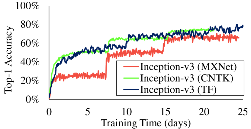
(a) Inception-v3

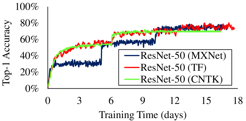
(b) ResNet-50

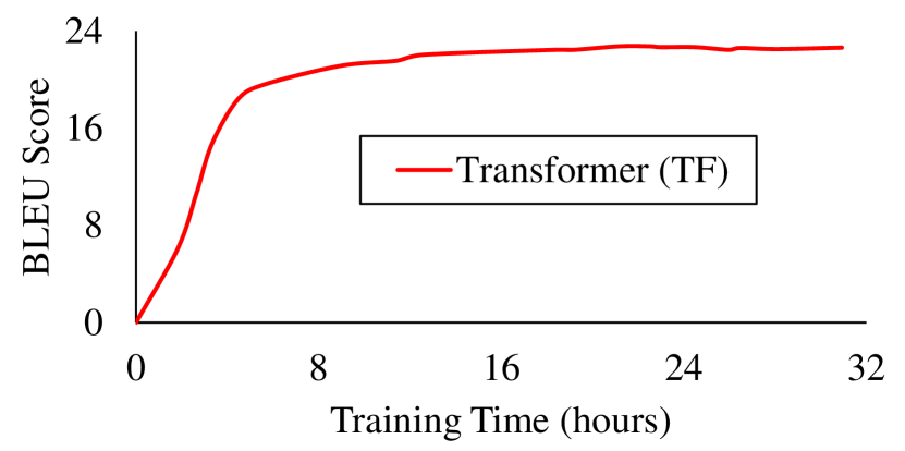
(c) Transformer

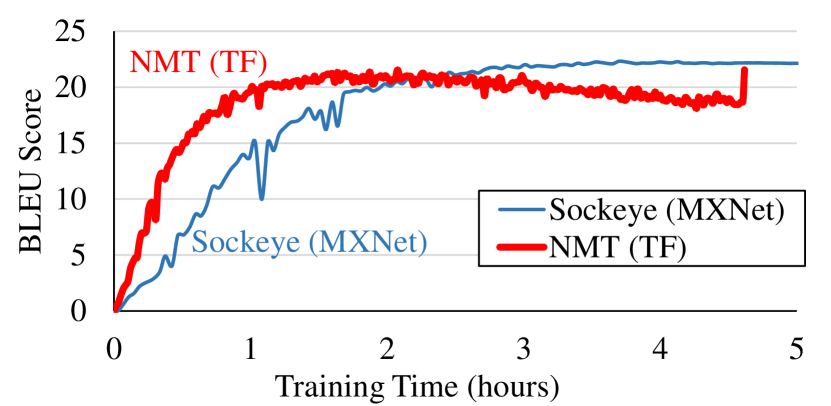
(d) Seq2Seq

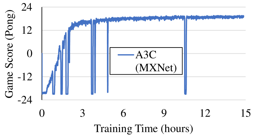
(e) A3C

Figure 2: The model accuracy during the training for different models.

To ensure that the results we obtain from our measurements are representative we need to verify that the training process for each model results in classification accuracy comparable to state of the art results published in the literature. To achieve this, we train the benchmark models in our suite until they converge to some expected accuracy rate (based on results from the literature).

Figure 2 shows the classification accuracy observed over time for five representative models in our benchmark suite, Inception-v3, ResNet-50, Seq2Seq, Transformer, and A3C, when trained on the single Quadro P4000 GPU hardware configuration described in Section 4. We observe that the training outcome of all models matches results in the literature. For the two image classification models (Inception-v3 and ResNet-50) the Top-1 classification accuracy reaches 75–80% and the the Top-5 accuracy is above 90%, both in agreement with previously reported results for these models  [52]. The accuracy of the machine translation models is measured using the BLEU score [73] metric, and we trained our model to achieve a BLEU score of around 20. For reinforcement learning, since the models are generally evaluated by Atari games, the accuracy of the A3C model is directly reflected by the score of the corresponding game. The A3C curve we show in this figure is from the Atari Pong game and matches previously reported results for that game (19–20) [70]. The training curve shape for different implementations of the same model on different frameworks can vary, but most of them usually converge to similar accuracy at the end of training.

3.4 Performance Analysis Framework and Tools

In this section we describe our analysis toolchain. This toolchain is designed to help us understand for each of the benchmarks, where the training time goes, how well the hardware resources are utilized and how to efficiently improve training performance.

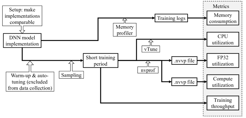
Figure 3: Analysis Pipeline

3.4.1 Making implementations comparable across frameworks

Implementations of the same model on different frameworks might vary in a few aspects that can impact performance profiling results. For example, different implementations might have hard-coded values for key hyper-parameters (e.g., learning rate, momentum, dropout rate, weight decay) in their code. To make sure that benchmarking identifies model-specific performance characteristics, rather than just implementation-specific details, we first adapt implementations of the same model to make them comparable across platforms. Besides making sure that all implementations run using the same model hyper-parameters, we also ensure that they define the same network, i.e. the same types and sizes of corresponding layers and layers are connected in the same way. Moreover, we make sure that the key properties of the training algorithm are the same across implementations. This is important for models, such as Faster R-CNN [82], where there are four different ways in which the training algorithm can share the internal weights.

3.4.2 Accurate and time-efficient profiling via sampling

The training of a deep neural network can take days or even weeks making it impractical to profile the entire training process. Fortunately, as the training process is an iterative algorithm and almost all the iterations follow the same computation logic, we find that accurate results can be obtained via sampling only for a short training period (on the order of minutes) out of the full training run. In our experiments, we sample 50-1000 iterations and collect the metrics of interest based on these iterations.

To obtain representative results, care must be taken when choosing the sample interval to ensure that the training process has reached stable state. Upon startup, a typical training procedure first goes through a warm-up phase (initializing for example the data flow graph, allocating memory and loading data) and then spends some time auto-tuning various parameters (e.g., system hyper-parameters, such as matrix multiplication algorithms, workspace size). Only after that the system enters the stable training phase for the remainder of the execution. While systems do not explicitly indicate when they enter the stable training phase, our experiments show that the warm-up and auto-tuning phase can be easily identified in measurements. We see that throughput stabilizes after several hundred iterations (a few thousand iterations in the case of Faster R-CNN). The sample time interval is then chosen after throughput has stabilized.

3.4.3 Relevant metrics

Below we describe the metrics we collect as part of the profiling process.

$\bullet$ Throughput: Advances in deep neural networks have been tightly coupled to the availability of compute resources capable of efficiently processing large training data sets. As such, a key metric when evaluating training efficiency is the number of input data samples that is being processed per second. We refer to this metric as throughput. Throughput is particularly relevant in the case of DNN training, since training, unlike inference, is not latency sensitive.

For the speech recognition model we slightly modify our definition of throughput. Due to the large variations in lengths among the audio data samples, we use the total duration of audio files processed per second instead of the number of files. The lengths of data samples also varies for machine translation models, but the throughput of these models is still stable so we use the throughput determined by simple counting for them.

$\bullet$GPU Compute Utilization: The GPU is the workhorse behind DNN training, as it is the unit responsible for executing the key operations involved in DNN training (broken down into basic operations such as vector and matrix operations). Therefore, for optimal throughput, the GPU should be busy all the time. Low utilization indicates that throughput is limited by other resources, such as CPU or data communication, and further improvement can be achieved by overlapping CPU runtime or data communication with GPU execution.

We define GPU Compute Utilization as the fraction of time that the GPU is busy (i.e. at least one of its typically many cores is active):

$$\text{GPU utilization}=\frac{\text{GPU active time}\times 100}{\text{total elapsed time}}\%$$ (1)

$\bullet$ FP32 utilization: We also look at GPU utilization from a different angle, measuring how effectively the GPU’s resources are being utilized while the GPU is active. More specifically, the training of DNNs is typically performed using single-precision floating point operations (FP32), so a key metric is how well the GPU’s compute potential for doing floating point operations is utilized. We compare the number of FP32 instructions the GPU actually executes while it is active to the maximal number of FP32 instructions it can theoretically execute during this time, to determine what percentage of its floating point capacity is utilized. More precisely, if a GPU’s theoretical peak capacity across all its cores is $FLOPS_{peak}$ single-precision floating point operations per second, we observe the actual number of floating point operations executed during a period of $T$ seconds that the GPU is active, to compute FP32 utilization as follows:

$$\text{FP32 utilization}=\frac{\text{actual flop count during T}\times 100}{FLOPS_{peak}\times T}\%$$ (2)

The FP32 utilization gives us a way to calculate the theoretical upper bound of performance improvements one could achieve by a better implementation. For example, an FP32 utilization of 50% indicates that we can increase throughput by up to 2x if we manage to increase the FP32 utilization up to 100%.

In addition to looking at the aggregate FP32 utilization across all cores, we also measure the per-core FP32 utilization for individual kernels, to identify the kernels with long duration, but low utilization. These kernels should be optimized with high priority.

$\bullet$ CPU utilization: While most of the training is typically performed on the GPU, the CPU is also involved, for example, to execute the framework frontends, launch GPU kernels, and transfer the data between CPU and GPU. We report CPU utilization as the average utilization across all cores:

$$\text{CPU utilization}=\frac{\sum_{c}{\text{total active time of core c}}\times 100}{\text{CPU core count}\times\text{total elapsed time}}\%$$ (3)

The ratio between the cumulative active time across all cores and total elapsed time is reported by vTune, so CPU utilization can be directly computed from there.

$\bullet$ Memory consumption: In addition to compute cycles, the amount of available physical memory has become a limiting factor in training large DNNs. In order to optimize memory usage during DNN training, it is important to understand where the memory goes, i.e. what data structures occupy most of the memory. Unfortunately, there are no open-source tools currently available for existing frameworks that can provide this analysis. Hence we build our own memory profilers for three main frameworks (TensorFlow, MXNet, and CNTK). We will open source these tools together with our benchmarks, as we expect them to be useful to others in developing and analyzing their models.

When building our memory profiler we carefully inspect how the different DNN frameworks in our benchmark allocate their memory and identify the data structures that are the main consumers of memory. We observe that most data structures are allocated before the training iterations start for these three frameworks. Each of the data structures usually belongs to one of the three types: weights, weight gradients and feature maps (similarly to prior works [83]). These data structures are allocated statically. In addition, a framework might allocate some workspace as a temporary container for intermediate results in a kernel function, which gives us another type of data structure. The allocation of workspace can be either static, before the training iterations, or dynamic, during the training iterations. We observe that in MXNet, data structures other than workspace are allocated during the training iterations (usually for the momentum computation) as well. We assign these data structures to a new type called ”dynamic”. As memory can be allocated and released during the training, we measure the memory consumption by the maximal amount of memory ever allocated for each type.

4 Evaluation

In this section, we use the methodology and framework described in the previous section for a detailed performance evaluation and analysis of the models in our TBD benchmark suite.

4.1 Experimental Setup

We use Ubuntu 16.04 OS, TensorFlow v1.3, MXNet v0.11.0, CNTK v2.0, with CUDA 8 and cuDNN 6. All of our experiments are carried out on a 16-machine cluster, where each node is equipped with a Xeon 28-core CPU and one to four NVidia Quadro P4000 GPUs. Machines are connected with both Ethernet and high speed Infiniband (100 Gb/sec) network cards.

As different GPU models provide a tradeoff between cost, performance, area and power, it is important to understand how different GPUs affect the key metrics in DNN training. We therefore also repeat a subset of our experiments using a second type of GPU, the NVidia TITAN Xp GPU. Table 4 compares the technical specifications of the two GPUs in our work. We show the comparative throughput and comparisons of our metrics between TITAN Xp and P4000 in Section 4.3.

	Titan Xp	Quadro P4000	Intel Xeon E5-2680
Multiprocessors	30	14
Core Count	3840	1792	28
Max Clock Rate (MHz)	1582	1480	2900
Memory Size (GB)	12	8	128
LLC Size (MB)	3	2	35
Memory Bus Type	GDDR5X	GDDR5	DDR4
Memory BW (GB/s)	547.6	243	76.8
Bus Interafce	PCIe 3.0	PCIe 3.0
Memory Speed (MHz)	5705	3802	2400

Table 4: Hardware specifications

4.2 Performance Analysis

As previously explained, our analysis will focus on a set of key metrics: throughput, GPU and CPU compute utilization, FP32 utilization, as well as a memory consumption breakdown.

Since one of the aspects that makes our work unique is the breadth in application domains, models and frameworks covered by our TBD benchmark suite we will pay particular attention to how the above metrics vary across applications, models and frameworks.

Moreover, we will use our setup to study the effects of a key hyper-parameter, the mini-batch size, on our metrics. It has been shown that to achieve high training throughput with the power of multiple GPUs using data parallelism, one must increase the mini-batch size, and additional work needs to be done on model parameters such as learning rate to preserve the training accuracy [43, 101]. In the single-GPU case, it is often assumed that larger mini-batch size will translate to higher GPU utilization, but the exact effects of varying mini-batch size are not well understood. In this work, we use our setup to quantify in detail how mini-batch size affects key performance metrics.

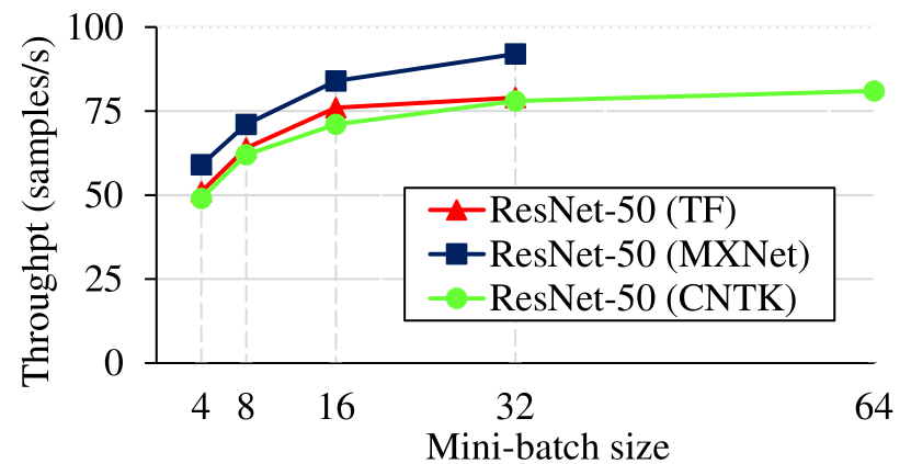
(a) ResNet-50

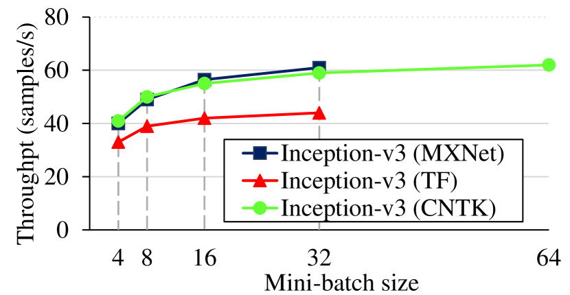
(b) Inception-v3

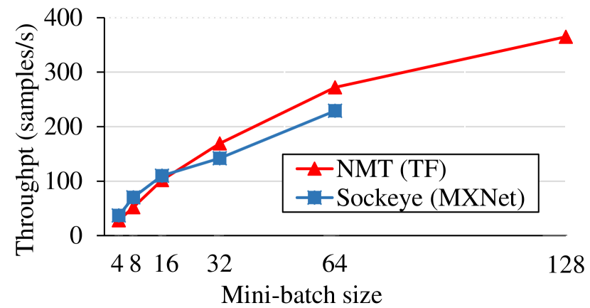
(c) Seq2Seq

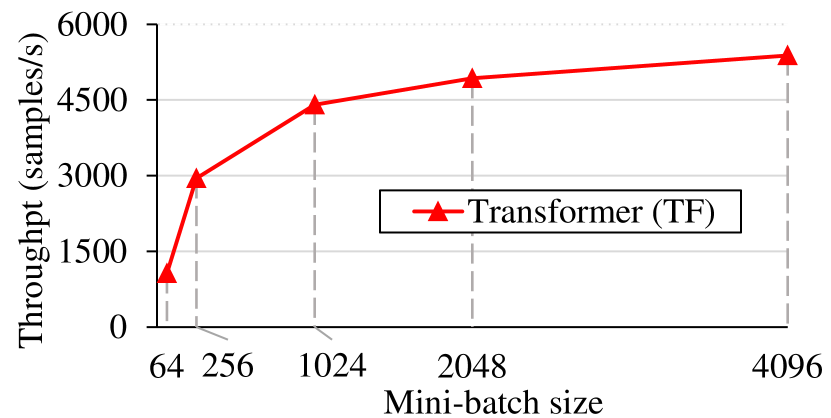
(d) Transformer

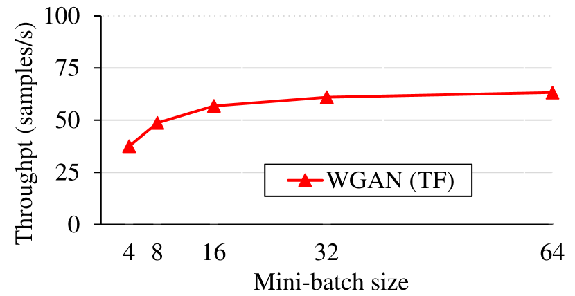
(e) WGAN

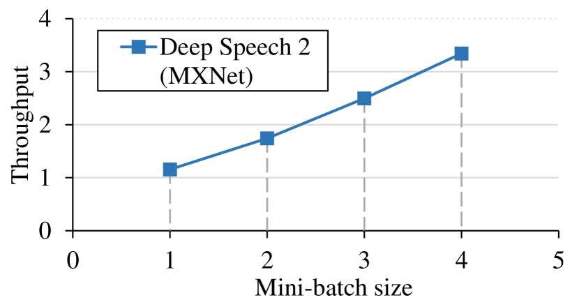
(f) Deep Speech 2

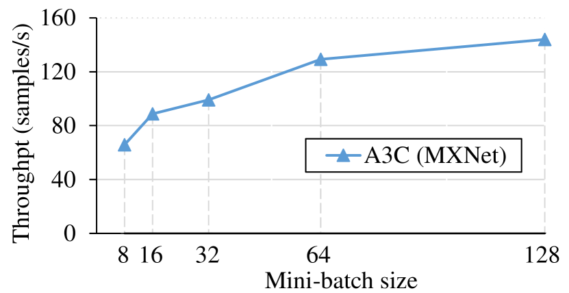
(g) A3C

Figure 4: DNN training throughput for different models on multiple mini-batch sizes.

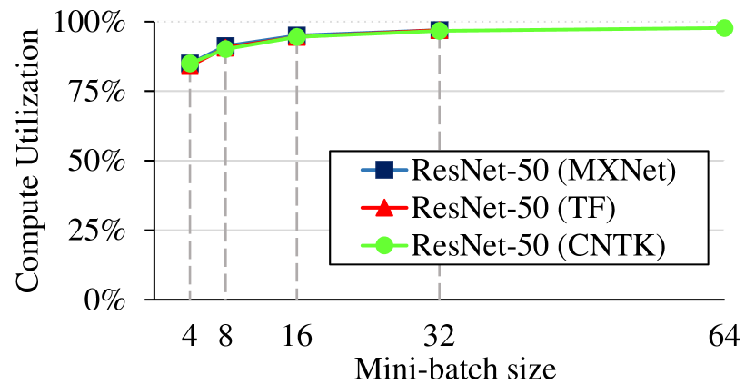
(a) ResNet-50

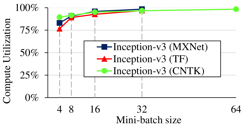
(b) Inception-v3

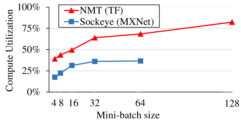
(c) Seq2Seq

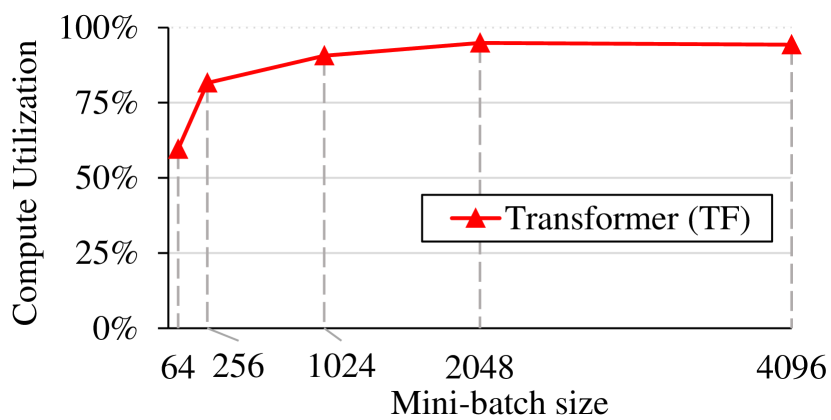
(d) Transformer

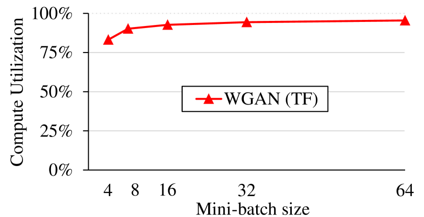
(e) WGAN

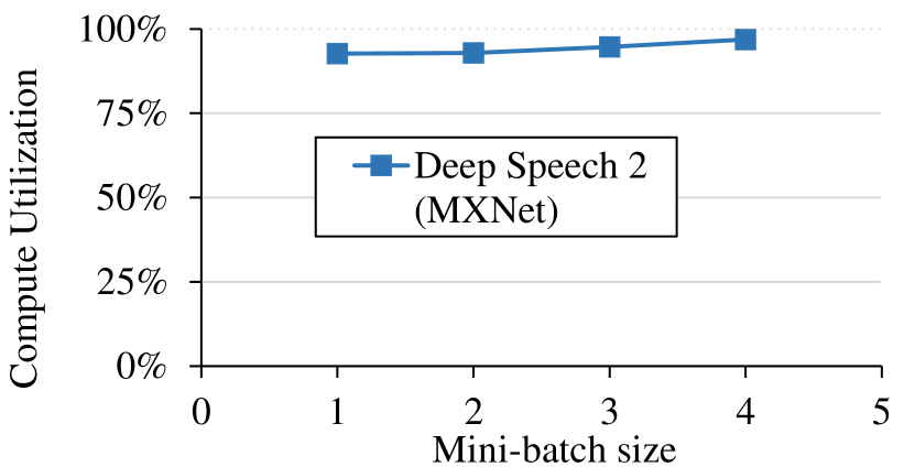
(f) Deep Speech 2

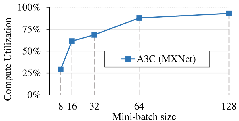
(g) A3C

Figure 5: GPU compute utilization for different models on multiple mini-batch sizes.

4.2.1 Throughput

Figure 4 shows the average training throughput for different models from the TBD suite when varying the mini-batch size (the maximum mini-batch size is limited by the GPU memory capacity). For Faster R-CNN, the number of images processed per iteration is fixed to be just one on a single GPU, hence we do not present a separate graph for Faster R-CNN. Both TensorFlow and MXNet implementations achieve a throughput of 2.3 images per second for Faster R-CNN. We make the following three observations from this figure.

Observation 1: Performance increases with the mini-batch size for all models. As we expected, the larger the mini-batch size, the higher the throughput for all models we study. We conclude that to achieve high training throughput on a single GPU, one should aim for a reasonably high mini-batch size, especially for non-convolutions models. We explain this behavior as we analyze the GPU and FP32 utilization metrics later in this section.

Observation 2: The performance of RNN-based models is not saturated within the GPU’s memory constraints. The relative benefit of further increasing the mini-batch size differs a lot between different applications. For example, for the NMT model increasing mini-batch size from 64 to 128 increases training throughput by 25%, and the training throughput of Deep Speech 2 scales almost linearly. These two models’ throughput (and hence performance) is essentially limited by the GPU memory capacity and we do not see any saturation point for them while increasing the mini-batch size. In contrast, other models also benefit from higher mini-batch size, but after certain saturation point these benefits are limited. For example, for the Inception-v3 model going from batch size of 16 to 32 has less than 10% in throughput improvement for implementations on all three frameworks.

Observation 3: Application diversity is important when comparing performance of different frameworks. We find that the results when comparing performance of models on different frameworks can greatly vary for different applications, and hence using a diverse set of applications in any comparisons of frameworks is important. For example, we observe that for image classification the MXNet implementations of both models (ResNet-50 and Inception-v3) perform generally better than the corresponding TensorFlow implementations, but at the same time, for machine translation the TensorFlow implementation of Seq2Seq (NMT) performs significalty better than its MXNet counterpart (Sockeye. TensorFlow also utilizes the GPU memory better than MXNet for Seq2Seq models so that it can be trained with a maximum mini-batch size of 128, while MXNet can only be trained with a maximum mini-batch of 64 (both limited by 8GB GPU memory). For the same memory budget, it allows TensorFlow achieve higher throughput, 365 samples per second, vs. 229 samples per second for MXNet. We conclude that there is indeed a signficant diversity on how different frameworks perform on different models, making it extremely important to study a diverse set of applications (and models) as we propose in our benchmark pool.

4.2.2 GPU Compute Utilization

Figure 5 shows the GPU compute utilization, the amount of time GPU is busy running some kernels (as formally defined by 3 in Section 3) for different benchmarks as we change the mini-batch size. Again, for Faster R-CNN, only batch of one is possible, and TensorFlow implementation achieves a relatively high compute utilization of 89.4% and the MXNet implementation achieves 90.3%. We make the following two observations from this figure.

Observation 4: The mini-batch size should be large enough to keep the GPU busy. Similar to our observation 1 about throughput, the larger the mini-batch size, the longer the duration of individual GPU kernel functions and the better the GPU compute utilization, as the GPU spends more time doing computations rather than invoking and finishing small kernels. While large mini-batch sizes also increase the overhead of data transfers, our results show that this overhead is usually efficiently parallelized with the computation.

Observation 5: The GPU compute utilization is low for LSTM-based models. Non-RNN models and Deep Speech 2 that uses regular RNN cells (not LSTM) usually reach very high utilization with large batches, around 95% or higher. Unfortunately, LSTM-based models (NMT, Sockeye) cannot drive up GPU utilization significantly, even with maximim mini-batch sizes. This means that, in general, these models do not utilize the available GPU hardware resources well, and further research should be done in how to optimize LSTM cells on GPUs. Moreover, it is important to notice that the low compute utilization problem is specific to the layer type, but not the application – the Transformer model also used in machine translation does not suffer from low compute utilization as it uses different (non-RNN) layer called Attention.

4.2.3 GPU FP32 utilization

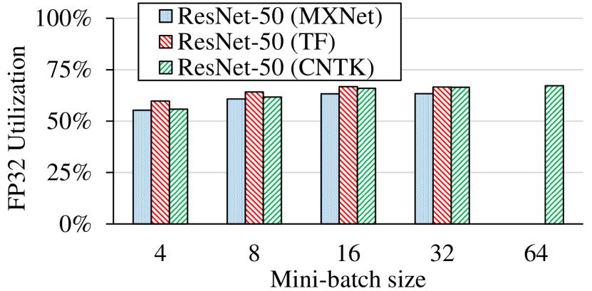
(a) ResNet-50

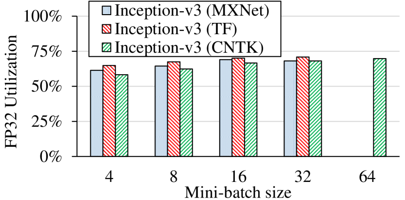
(b) Inception-v3

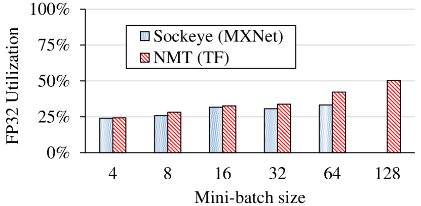
(c) Seq2Seq

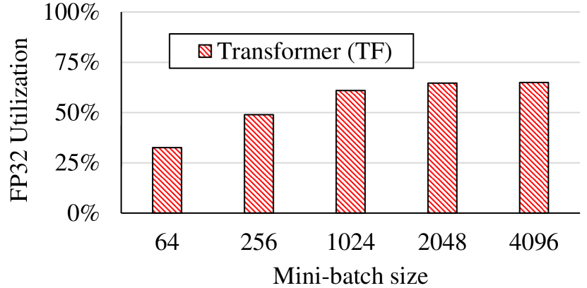
(d) Transformer

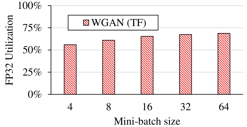
(e) WGAN

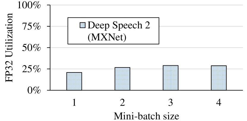
(f) Deep Speech 2

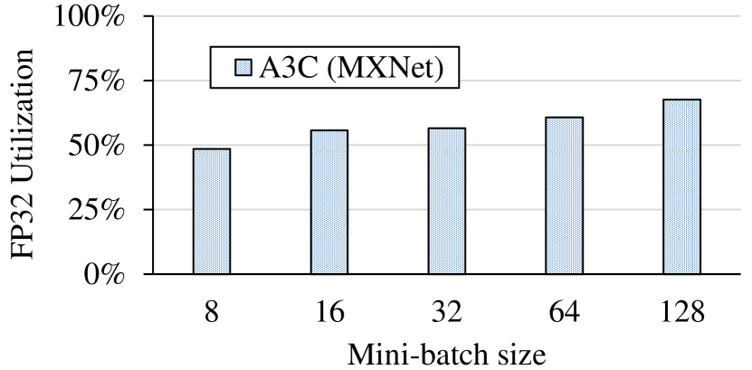
(g) A3C

Figure 6: GPU FP32 utilization for different models on multiple mini-batch sizes.

Figure 6 shows the GPU FP32 utilization (formally defined by 2 in Section 3) for different benchmarks as we change the mini-batch size (until memory capacity permits). For Faster R-CNN, the MXNet/TensforFlow implementations achieve an average utilization of 70.9%/58.9% correspondingly. We make three major observations from this figure.

Observation 6: The mini-batch size should be large enough to exploit the FP32 computational power of GPU cores. As expected, we observe that large mini-batch sizes also improve GPU FP32 utilization for all benchmarks we study. We conclude that both the improved FP32 utilization (Observation 6) and GPU utilization (Observation 4) are key contributors to the increases in overall throughput with the mini-batch size (Observation 1).

Observation 7: RNN-based models have low GPU FP32 utilization. Even with the maximum mini-batch size possible (on a single GPU), the GPU FP32 utilization of the two RNN-based models (Seq2Seq and Deep Speech 2, Figure 6(c) and Figure 6(f), respectively) are much lower than for other non-RNN models. This clearly indicates the potential of designing more efficient RNN layer implementations used in TensforFlow and MXNet, and we believe further research should be done to understand the sources of these inefficiences. Together with Observation 5 (low GPU utilization for LSTM-based models) this observation explains why in Observation 2 we do not observe throughput saturation for RNN-based models even for very large mini-batches.

Observation 8: There exists kernels with long duration, but low FP32 utilization even for highly optimized models. The previous observation might have brought up the question why average FP32 utilizations are so low, even for extremely optimized CNN models. In this observation we provide an answer: Different kernels vary greatly in their FP32 utilizations, and even optimized models have long-running kernels with low utilization. Table 5 and Table 6 show the five most important kernels with the FP32 utilization lower than average (for ResNet-50 model on TensorFlow and MXNet). We observe that the cuDNN batch normalization kernels (have bn part in their names) are the major source of inefficiency with FP32 utilizations more than 20% below the average. Note that this observation is true for implementations on different frameworks. If we want to get further progress in improving DNN training performance on GPUs, these kernels are the top candidates for acceleration.

Duration	Utilization	Kernel Name
8.36%	30.0%	magma_lds128_sgemm_kernel…
5.53%	42.3%	cudnn::detail::bn_bw_1C11_kernel_new…
4.65%	46.3%	cudnn::detail::bn_fw_tr_1C11_kernel_new…
3.12%	20.0%	Eigen::internal::EigenMetaKernel…
2.48%	40.0%	tensorflow::BiasNHWCKernel…

Table 5: Longest 5 kernels with utilization level below the average (ResNet-50, mini-batch size 32, TensorFlow)

Duration	Utilization	Kernel Name
9.43%	30.0%	cudnn::detail::bn_bw_1C11_kernel_new…
7.96%	42.3%	cudnn::detail::bn_fw_tr_1C11_kernel_new…
5.14%	46.3%	cudnn::detail::activation_bw_4d_kernel…
3.52%	20.0%	cudnn::detail::activation_fw_4d_kernel…
2.85%	40.0%	_ZN5mxnet2op8mxnet_op20mxnet_generic_kernel…

Table 6: Longest 5 kernels with FP32 utilization below the average (ResNet-50, mini-batch size 32, MXNet)

4.2.4 CPU Utilization

The results of our analysis of CPU utilization are presented in Figure 7.

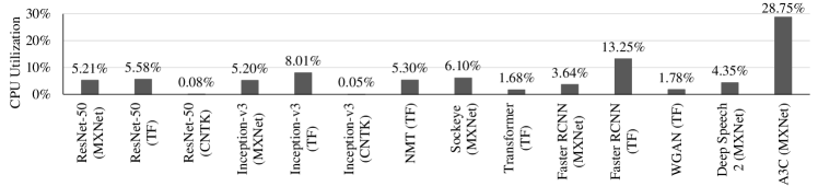
Figure 7: Average CPU utilization for different models.

Observation 9: CPU utilization is low in DNN training. We observe that for all our models the CPU utilization is very low, less than 15% for all but one model, less than 8% for all but two models. For our CPU machines with 28 cores, this means that on average less than 2 cores are usually busy. We believe that future research should look into how to make CPUs more useful for DNN training. For example, they can be used to compute layers that cannot benefit from the massive GPU compute power, such as batch normalization.

4.3 Hardware Sensitivity

The results presented so far, were based on experiments with the Quadro P4000 GPU. In this section we are interested in seeing how the performance of DNN training will depend on the hardware used. Toward this end we compare the training throughput, GPU utilization, and FP32 utilization for several of our models: ResNet-50, Inception-v3, and Seq2Seq on P4000 GPU and the more powerful Titan Xp GPU. For throughput comparison, we normalized each model result to the throughput of less powerfull P4000 card. We make the following observation from this figure.

Observation 10: More advanced GPUs should be accompanied by better systems designs and more efficient low-level libraries. Titan Xp usually helps improving the training throughput (except for Sockeye), however the computation power of Titan Xp is not well-utilized. Both the GPU and the FP32 utilizations of Titan Xp appear to be worse than those of P4000. Hence we conclude that although Titan Xp is more computationally powerful (more multiprocessors, CUDA cores, and bandwidth, see Table 4), the proper utilization of these resources requires a more careful design of existing GPU kernel functions, libraries (e.g., cuDNN), and algorithms that can efficiently exploit these resources.

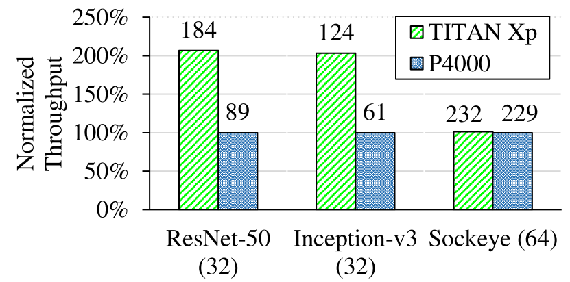
(a) MXNet

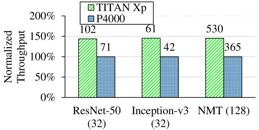
(b) TensorFlow

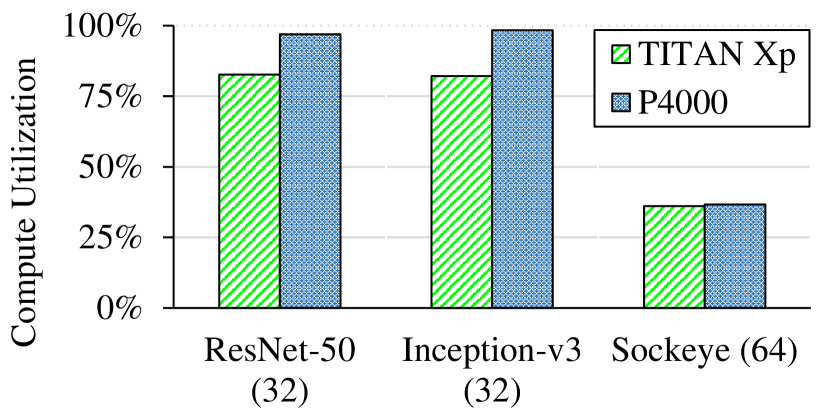
(c) MXNet

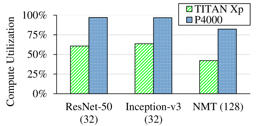
(d) TensorFlow

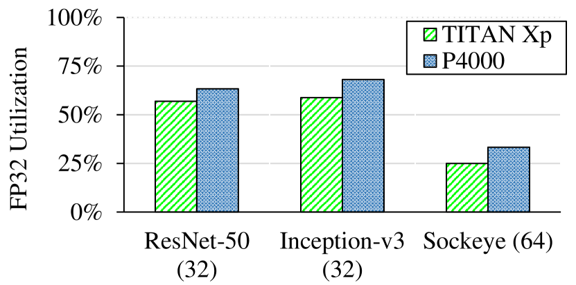
(e) MXNet

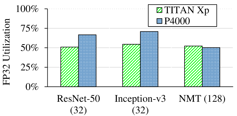
(f) TensorFlow

Figure 8: Throughput, Compute Utilization, FP32 Utilization comparison between P4000 and Titan Xp for different benchmarks.

4.4 Memory Profiling

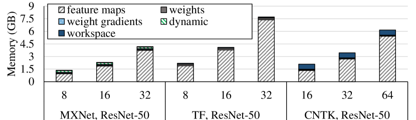
(a) ResNet-50

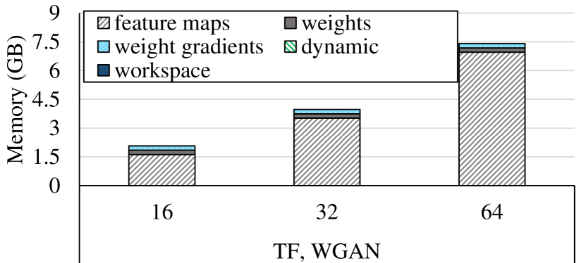
(b) WGAN

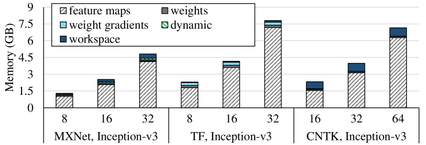
(c) Inception-v3

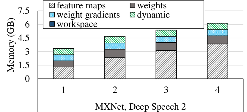
(d) Deep Speech 2

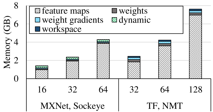
(e) Seq2Seq

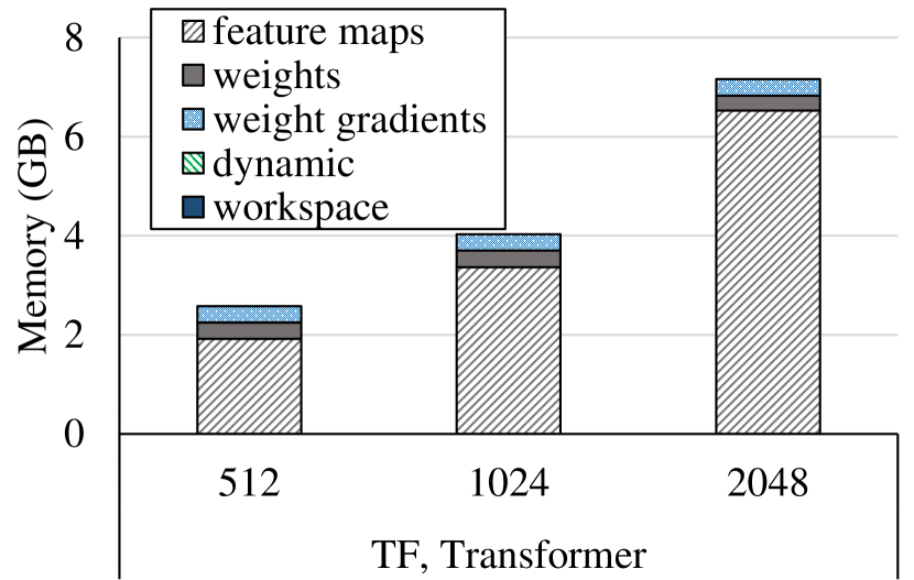
(f) Transformer

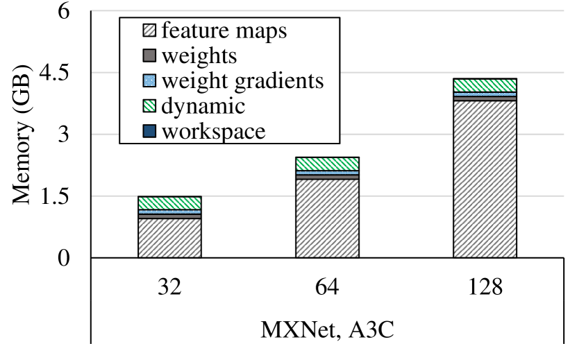
(g) A3C

Figure 9: GPU memory usage breakdown for different models on multiple mini-batch sizes.

As we have previously shown, the throughput (and hence the performance) of DNN training can be significantly bottlenecked by the available GPU memory. Figure 9 shows the result of our analysis where the memory is separated in five categories: weights, gradient weights, feature maps, dynamic, and workspace. Where appropriate, we vary the size of the mini-batch (shown in parentheses). The Faster R-CNN model results are similar to image classification models, but only support one batch size (hence we do not plot them in a separate graph).

Observation 11: Feature maps are the dominant consumers of memory. It turns out that feature maps (intermediate layer outpus) are the dominant part of the memory consumption, rather than weights, which are usually the primary focus of memory optimization for inference. The total amount of memory consumed by feature maps ranges from 62% in Deep Speech 2 to 89% in ResNet-50 and Sockeye. Hence any optimization that wants to reduce the memory footprint of training should, first of all, focus on feature maps. This is an interesting observation also because it expands on the results reported in the only prior work reporting on memory consumption breakdown for DNN training by Rhu et al. [83]. They look at CNN training only and find that weights are only responsible for a very small portion of the total memory footprint. We extend this observation outside of CNNs, but also observe that there are models (e.g., Deep Speech 2) where weights are equally important.

Observation 12: Simply exhausting GPU memory with large mini-batch size might be inefficient. The memory consumption of feature maps scales almost linearly with the mini-batch size. From observation 11, we know that reducing the mini-batch size can dramatically reduce the overall memory consumption needed for training. Based on observation 1, we also know that the side-effect of throughput loss while reducing the mini-batch size can be acceptable (for non-RNN models) until you do not go below saturation point. One can use the additional GPU memory for larger workspace (can be used for faster implementation of matrix multiplications or convolutions) and deeper models (e.g., ResNet-102 vs. ResNet-50).

4.5 Multi-GPU and Multi-Machine Training

Training large DNNs can be done faster when multiple GPUs and/or multiple machines are used. This is usually achieved by using data parallelism, where mini-batches are split between individual GPUs and the results are then merged, for example, using the parameter server approach [66]. But in order to realize the computational potential of multiple GPUs the comminication channels between them need to have sufficient bandwidth to exchange proper weight updates. In our work, we decide to analyze the performance scalability of DNN training using multiple GPUs and multiple machines. We use the ResNet-50 model on MXNet to perform this analysis. Figure 10 shows the results of our experiment. *M stands for the number of machines, and *G for the number of GPUs.

Observation 13: Network bandwidth must be large enough for good scalability. We observe that going from the one machine (1M1G) to the two machine (2M1G (ethernet)) coniguration the performance degrades significantly. This is because DNN training requires constant synchronization between GPUs in distributed training. Hence faster networking is required to improve the situation (the 2M1G (infiniband) coniguration has 100Gb/s IniniBand Mellanox networking). In contrast, DNN training on a single machine with multiple GPUs (1M1G, 1M2G, 1M4G) scales reasonably well as PCIe 3.0 gives enough bandwidth (16 GB/s)s. In summary, this suggests that networking bandwidth is critical for performance of distributed training and different techniques (in both software and hardware) should be applied to either reduce the amount of data sent or increase the available bandwidth.

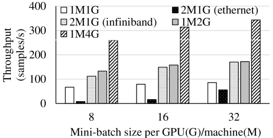
Figure 10: ResNet-50 on MXNet with multiple GPUs/machines.

5 Related Work

There are only a handful of existing open-source DNN benchmark projects, each with a focus that is very different from our work. ConvNet [3], CNN-benchmarks [2] and Shaohuai et al. [89] focus exclusively on convolutional network models mainly for image classification based on the ImageNet data, with the only exception being one LSTM network in  [89]. In contrast the goal of our work is a benchmark that covers a wide range of models and applications, beyond just CNNs and image classification.

DeepBench [5] is an open-source project from Baidu Research, which is targeted at a lower level in the deep learning stack than our work: rather than working with implementations of deep learning models and frameworks, it instead benchmarks the performance of individual lower level operations (e.g. matrix multiplication) as implemented in libraries used by various frameworks and directly executed against the underlying hardware.

The Eyeriss project [1] presents evaluations of a few DNN processors [26, 46] on hardware metrics for several convolutional networks, but their work is focused on inference, while ours targets training.

Among existing work, Fathom [11] is probably the one closest to our own, as it also focuses on training and more than a single application (machine translation, speech recognition and reinforcement learning). However, their focus is on micro-architectural aspects of execution, breaking down training time into time spent on the various operation types (e.g. matrix multiplication). In contrast, our benchmark pool focuses on system level aspects of execution such as throughput, hardware utilization, and memory consumption profiling. Moreover, Fathom is based on only one framework (TensorFlow), does not consider distributed training and uses models that are somewhat out-dated by now.

Driven by the achievements of DNN algorithms and the availability of large datasets, many frameworks [10, 20, 24, 102, 59, 93, 32, 30, 76] were recently proposed for users to easily develop new DNN models for different application domains. These frameworks provide high-level numpy-like APIs or layer-wise configuration files to promote programmability. They are also able to make use of modern hardware accelerators (especially GPUs) to speed up the DNN training process. In our work, we use three of these frameworks: TensorFlow [10], MXNet [24], and CNTK [102], but we envision to add more frameworks with more models as we keep developing our benchmark pool and based on the feedback we expect from both academia and industry.

Due to the complexity of DNN computations, ML developers usually need additional profiling tools to understand the training performance characteristics. Some frameworks have their own profiling tools embedded. For example, MXNet allows users to see the timeline for individual layers. However, this layer-level representation hides details inside a layer computation, and provide little information about efficiency of GPU computation. We therefore use the NVIDIA profiling tool called nvprof [9], which enables detailed performance information for each GPU kernel. It also shows a timeline of both CPU and GPU activities at the function/kernel level. Another end-to-end profiling tool we use is the Intel VTune [80] Amplifier. It provides detailed analysis of CPU performance (e.g., identifies the “hotspots”, where the application spends a lot of time) and also supports the metrics we need. At the same time, we can not use these tools directly on the full training process due to memory and time limits, and has to adopt these tools for our need as described in Section 3.

To exploit the GPU computation power and to reduce the programming effort, there are several GPU libraries that provide efficient implementation of basic operations on vectors and multi-dimension matrices. The most notable examples include cuDNN [27] and cuBLAS [4] by NVIDIA, MKL [96] by Intel, and Eigen [6]. NVIDIA also provides the NCCL library [7] which implements multi-GPU and multi-node communication primitives to reduce communication overhead among GPUs. These libraries are widely employed by most mainstream deep learning frameworks and the three frameworks we use in this work (TensorFlow, MXNet, and CNTK). These libraries greatly affect the overall training performance, and hence are an important target of performance analysis and tuning.

Multiple techniques are proposed to reduce the memory usage of DNN, including network pruning [49, 65, 50, 47, 48], parameter quantizing or precision reducing [47, 16, 40, 33, 78].

These are extremely useful for inference since they are very effective in reducing the memory footprint of weights, which enables DNN inference in mobile environment. Rhu et al. [83] has shown that for the state-of-the-art CNN training, weights are only responsible for a very small portion of total memory footprint. We extend this observation outside of CNNs, but also show that there are models (e.g., Deep Speech 2) where weights are equally important. Algorithms designed for training DNN with quantized values [33, 48, 40] suffer from accuracy loss for state-of-the-art models on large datasets. Rhu et al. [83] develops a new mechanism which uses CPU memory as a temporary container for feature maps, which greatly reduces the memory footprint of DNN training.

They also developed a tool to show the GPU memory usage for different data structures, but, unfortunately, this tool is not available outside of NVIDIA. In this work, we aim to build efficient memory profilers that will be available to a wider community as we open source them.

6 Conclusion

In this work, we proposed a new benchmark suite for DNN training, called TBD, that covers a wide range of machine applications from image classification and machine translation to reinforcement learning. TBD consists of eight state-of-the-art DNN models implemented on major deep learning frameworks such as TensorFlow, MXNet, and CNTK. We used these models to perform extensive performance analysis and profiling to shed light on efficiency of DNN training for different hardware configurations (single-/multi-GPU and multi-machine). We developed a new tool chain for end-to-end analysis of DNN training that includes (i) piecewise profiling of specific parts of training using existing performance analysis tools, and (ii) merging and analyzing the results from these tools using the domain-specific knowledge of DNN training. Additionally, we built new memory profiling tools specifically for DNN training for all three major frameworks. These useful tools can precisely characterize where the memory consumption (one of the major bottlenecks in training DNNs) goes and how much memory is consumed by key data structures (weights, activations, gradients, workspace). By using our tools and methodologies, we made several important observations and recommendations on where the future research and optimization of DNN training should be focused. We hope that our TBD benchmark suite, tools, methodologies, and observations will be useful for a large number of ML developers and systems designers in making their DNN training process efficient.

References

- [1] Benchmarking dnn processors. http://eyeriss.mit.edu/benchmarking.html.
- [2] cnn-benchmarks. https://github.com/jcjohnson/cnn-benchmarks.
- [3] convnet-benchmarks. https://github.com/soumith/convnet-benchmarks.
- [4] cublas. http://docs.nvidia.com/cuda/cublas/index.html.
- [5] Deepbench. https://github.com/baidu-research/DeepBench.
- [6] Eigen: A c++ linear algebra library. http://eigen.tuxfamily.org/index.php?title=Main_Page.
- [7] Nvidia collective communications library (nccl). https://developer.nvidia.com/nccl.
- [8] Nvidia geforce gtx 580. https://www.geforce.com/hardware/desktop-gpus/geforce-gtx-580.
- [9] Nvidia visual profiler’s user guide. http://docs.nvidia.com/cuda/profiler-users-guide/index.html.
- [10] Martín Abadi, Paul Barham, Jianmin Chen, Zhifeng Chen, Andy Davis, Jeffrey Dean, Matthieu Devin, Sanjay Ghemawat, Geoffrey Irving, Michael Isard, et al. Tensorflow: A system for large-scale machine learning. In OSDI, volume 16, pages 265–283, 2016.
- [11] Robert Adolf, Saketh Rama, Brandon Reagen, Gu-Yeon Wei, and David Brooks. Fathom: reference workloads for modern deep learning methods. In Workload Characterization (IISWC), 2016 IEEE International Symposium on, pages 1–10. IEEE, 2016.
- [12] Jorge Albericio, Alberto Delmás, Patrick Judd, Sayeh Sharify, Gerard O’Leary, Roman Genov, and Andreas Moshovos. Bit-pragmatic deep neural network computing. In Proceedings of the 50th Annual IEEE/ACM International Symposium on Microarchitecture, pages 382–394. ACM, 2017.
- [13] Jorge Albericio, Patrick Judd, Tayler Hetherington, Tor Aamodt, Natalie Enright Jerger, and Andreas Moshovos. Cnvlutin: ineffectual-neuron-free deep neural network computing. In Computer Architecture (ISCA), 2016 ACM/IEEE 43rd Annual International Symposium on, pages 1–13. IEEE, 2016.
- [14] Manoj Alwani, Han Chen, Michael Ferdman, and Peter Milder. Fused-layer cnn accelerators. In Microarchitecture (MICRO), 2016 49th Annual IEEE/ACM International Symposium on, pages 1–12. IEEE, 2016.
- [15] Dario Amodei, Sundaram Ananthanarayanan, Rishita Anubhai, Jingliang Bai, Eric Battenberg, Carl Case, Jared Casper, Bryan Catanzaro, Qiang Cheng, Guoliang Chen, et al. Deep speech 2: End-to-end speech recognition in english and mandarin. In International Conference on Machine Learning, pages 173–182, 2016.
- [16] Sajid Anwar, Kyuyeon Hwang, and Wonyong Sung. Fixed point optimization of deep convolutional neural networks for object recognition. In Acoustics, Speech and Signal Processing (ICASSP), 2015 IEEE International Conference on, pages 1131–1135. IEEE, 2015.
- [17] Martin Arjovsky, Soumith Chintala, and Léon Bottou. Wasserstein gan. arXiv preprint arXiv:1701.07875, 2017.
- [18] Dzmitry Bahdanau, Kyunghyun Cho, and Yoshua Bengio. Neural machine translation by jointly learning to align and translate. arXiv preprint arXiv:1409.0473, 2014.
- [19] Yoshua Bengio, Pascal Lamblin, Dan Popovici, and Hugo Larochelle. Greedy layer-wise training of deep networks. In Advances in neural information processing systems, pages 153–160, 2007.
- [20] James Bergstra, Olivier Breuleux, Frédéric Bastien, Pascal Lamblin, Razvan Pascanu, Guillaume Desjardins, Joseph Turian, David Warde-Farley, and Yoshua Bengio. Theano: A cpu and gpu math compiler in python. In Proc. 9th Python in Science Conf, pages 1–7, 2010.
- [21] Mariusz Bojarski, Davide Del Testa, Daniel Dworakowski, Bernhard Firner, Beat Flepp, Prasoon Goyal, Lawrence D Jackel, Mathew Monfort, Urs Muller, Jiakai Zhang, et al. End to end learning for self-driving cars. arXiv preprint arXiv:1604.07316, 2016.
- [22] Mahdi Nazm Bojnordi and Engin Ipek. Memristive boltzmann machine: A hardware accelerator for combinatorial optimization and deep learning. In High Performance Computer Architecture (HPCA), 2016 IEEE International Symposium on, pages 1–13. IEEE, 2016.
- [23] Mauro Cettolo, Jan Niehues, Sebastian Stüker, Luisa Bentivogli, Roldano Cattoni, and Marcello Federico. The iwslt 2015 evaluation campaign. In IWSLT 2015, International Workshop on Spoken Language Translation, 2015.
- [24] Tianqi Chen, Mu Li, Yutian Li, Min Lin, Naiyan Wang, Minjie Wang, Tianjun Xiao, Bing Xu, Chiyuan Zhang, and Zheng Zhang. Mxnet: A flexible and efficient machine learning library for heterogeneous distributed systems. arXiv preprint arXiv:1512.01274, 2015.
- [25] Yu-Hsin Chen, Joel Emer, and Vivienne Sze. Eyeriss: A spatial architecture for energy-efficient dataflow for convolutional neural networks. In Computer Architecture (ISCA), 2016 ACM/IEEE 43rd Annual International Symposium on, pages 367–379. IEEE, 2016.
- [26] Yu-Hsin Chen, Tushar Krishna, Joel S Emer, and Vivienne Sze. Eyeriss: An energy-efficient reconfigurable accelerator for deep convolutional neural networks. IEEE Journal of Solid-State Circuits, 52(1):127–138, 2017.
- [27] Sharan Chetlur, Cliff Woolley, Philippe Vandermersch, Jonathan Cohen, John Tran, Bryan Catanzaro, and Evan Shelhamer. cudnn: Efficient primitives for deep learning. arXiv preprint arXiv:1410.0759, 2014.
- [28] Ping Chi, Shuangchen Li, Cong Xu, Tao Zhang, Jishen Zhao, Yongpan Liu, Yu Wang, and Yuan Xie. Prime: A novel processing-in-memory architecture for neural network computation in reram-based main memory. In Proceedings of the 43rd International Symposium on Computer Architecture, pages 27–39. IEEE Press, 2016.
- [29] Trishul M Chilimbi, Yutaka Suzue, Johnson Apacible, and Karthik Kalyanaraman. Project adam: Building an efficient and scalable deep learning training system. In OSDI, volume 14, pages 571–582, 2014.
- [30] François Chollet et al. Keras. https://github.com/fchollet/keras, 2015.
- [31] Patryk Chrabaszcz, Ilya Loshchilov, and Frank Hutter. A downsampled variant of imagenet as an alternative to the cifar datasets. arXiv preprint arXiv:1707.08819, 2017.
- [32] Ronan Collobert, Koray Kavukcuoglu, and Clément Farabet. Torch7: A matlab-like environment for machine learning. In BigLearn, NIPS workshop, number EPFL-CONF-192376, 2011.
- [33] Matthieu Courbariaux, Yoshua Bengio, and Jean-Pierre David. Binaryconnect: Training deep neural networks with binary weights during propagations. In Advances in neural information processing systems, pages 3123–3131, 2015.
- [34] Paul Covington, Jay Adams, and Emre Sargin. Deep neural networks for youtube recommendations. In Proceedings of the 10th ACM Conference on Recommender Systems, pages 191–198. ACM, 2016.
- [35] Christopher De Sa, Matthew Feldman, Christopher Ré, and Kunle Olukotun. Understanding and optimizing asynchronous low-precision stochastic gradient descent. In Proceedings of the 44th Annual International Symposium on Computer Architecture, pages 561–574. ACM, 2017.
- [36] Jeffrey Dean, Greg Corrado, Rajat Monga, Kai Chen, Matthieu Devin, Mark Mao, Andrew Senior, Paul Tucker, Ke Yang, Quoc V Le, et al. Large scale distributed deep networks. In Advances in neural information processing systems, pages 1223–1231, 2012.
- [37] Caiwen Ding, Siyu Liao, Yanzhi Wang, Zhe Li, Ning Liu, Youwei Zhuo, Chao Wang, Xuehai Qian, Yu Bai, Geng Yuan, et al. C ir cnn: accelerating and compressing deep neural networks using block-circulant weight matrices. In Proceedings of the 50th Annual IEEE/ACM International Symposium on Microarchitecture, pages 395–408. ACM, 2017.
- [38] Zidong Du, Daniel D Ben-Dayan Rubin, Yunji Chen, Liqiang He, Tianshi Chen, Lei Zhang, Chengyong Wu, and Olivier Temam. Neuromorphic accelerators: A comparison between neuroscience and machine-learning approaches. In Proceedings of the 48th International Symposium on Microarchitecture, pages 494–507. ACM, 2015.
- [39] Zidong Du, Robert Fasthuber, Tianshi Chen, Paolo Ienne, Ling Li, Tao Luo, Xiaobing Feng, Yunji Chen, and Olivier Temam. Shidiannao: Shifting vision processing closer to the sensor. In ACM SIGARCH Computer Architecture News, volume 43, pages 92–104. ACM, 2015.
- [40] Steve K Esser, Rathinakumar Appuswamy, Paul Merolla, John V Arthur, and Dharmendra S Modha. Backpropagation for energy-efficient neuromorphic computing. In Advances in Neural Information Processing Systems, pages 1117–1125, 2015.
- [41] Mark Everingham, Luc Van Gool, Christopher KI Williams, John Winn, and Andrew Zisserman. The pascal visual object classes (voc) challenge. International journal of computer vision, 88(2):303–338, 2010.
- [42] Mingyu Gao, Jing Pu, Xuan Yang, Mark Horowitz, and Christos Kozyrakis. Tetris: Scalable and efficient neural network acceleration with 3d memory. In Proceedings of the Twenty-Second International Conference on Architectural Support for Programming Languages and Operating Systems, pages 751–764. ACM, 2017.
- [43] Priya Goyal, Piotr Dollár, Ross Girshick, Pieter Noordhuis, Lukasz Wesolowski, Aapo Kyrola, Andrew Tulloch, Yangqing Jia, and Kaiming He. Accurate, large minibatch sgd: Training imagenet in 1 hour. arXiv preprint arXiv:1706.02677, 2017.
- [44] Yijin Guan, Zhihang Yuan, Guangyu Sun, and Jason Cong. Fpga-based accelerator for long short-term memory recurrent neural networks. In Design Automation Conference (ASP-DAC), 2017 22nd Asia and South Pacific, pages 629–634. IEEE, 2017.
- [45] Ishaan Gulrajani, Faruk Ahmed, Martin Arjovsky, Vincent Dumoulin, and Aaron C Courville. Improved training of wasserstein gans. In Advances in Neural Information Processing Systems, pages 5769–5779, 2017.
- [46] Song Han, Xingyu Liu, Huizi Mao, Jing Pu, Ardavan Pedram, Mark A Horowitz, and William J Dally. Eie: efficient inference engine on compressed deep neural network. In Proceedings of the 43rd International Symposium on Computer Architecture, pages 243–254. IEEE Press, 2016.
- [47] Song Han, Huizi Mao, and William J Dally. Deep compression: Compressing deep neural networks with pruning, trained quantization and huffman coding. arXiv preprint arXiv:1510.00149, 2015.
- [48] Song Han, Jeff Pool, John Tran, and William Dally. Learning both weights and connections for efficient neural network. In Advances in neural information processing systems, pages 1135–1143, 2015.
- [49] Stephen José Hanson and Lorien Y Pratt. Comparing biases for minimal network construction with back-propagation. In Advances in neural information processing systems, pages 177–185, 1989.
- [50] Babak Hassibi and David G Stork. Second order derivatives for network pruning: Optimal brain surgeon. In Advances in neural information processing systems, pages 164–171, 1993.
- [51] Johann Hauswald, Yiping Kang, Michael A Laurenzano, Quan Chen, Cheng Li, Trevor Mudge, Ronald G Dreslinski, Jason Mars, and Lingjia Tang. Djinn and tonic: Dnn as a service and its implications for future warehouse scale computers. In ACM SIGARCH Computer Architecture News, volume 43, pages 27–40. ACM, 2015.
- [52] Kaiming He, Xiangyu Zhang, Shaoqing Ren, and Jian Sun. Deep residual learning for image recognition. In Proceedings of the IEEE conference on computer vision and pattern recognition, pages 770–778, 2016.
- [53] Xiangnan He, Lizi Liao, Hanwang Zhang, Liqiang Nie, Xia Hu, and Tat-Seng Chua. Neural collaborative filtering. In Proceedings of the 26th International Conference on World Wide Web, pages 173–182. International World Wide Web Conferences Steering Committee, 2017.
- [54] Felix Hieber, Tobias Domhan, Michael Denkowski, David Vilar, Artem Sokolov, Ann Clifton, and Matt Post. Sockeye: A toolkit for neural machine translation. arXiv preprint arXiv:1712.05690, 2017.
- [55] Geoffrey E Hinton, Simon Osindero, and Yee-Whye Teh. A fast learning algorithm for deep belief nets. Neural computation, 18(7):1527–1554, 2006.
- [56] Kevin Hsieh, Aaron Harlap, Nandita Vijaykumar, Dimitris Konomis, Gregory R Ganger, Phillip B Gibbons, and Onur Mutlu. Gaia: Geo-distributed machine learning approaching lan speeds. In NSDI, pages 629–647, 2017.
- [57] Brody Huval, Tao Wang, Sameep Tandon, Jeff Kiske, Will Song, Joel Pazhayampallil, Mykhaylo Andriluka, Pranav Rajpurkar, Toki Migimatsu, Royce Cheng-Yue, et al. An empirical evaluation of deep learning on highway driving. arXiv preprint arXiv:1504.01716, 2015.
- [58] Yu Ji, YouHui Zhang, ShuangChen Li, Ping Chi, CiHang Jiang, Peng Qu, Yuan Xie, and WenGuang Chen. Neutrams: Neural network transformation and co-design under neuromorphic hardware constraints. In Microarchitecture (MICRO), 2016 49th Annual IEEE/ACM International Symposium on, pages 1–13. IEEE, 2016.
- [59] Yangqing Jia, Evan Shelhamer, Jeff Donahue, Sergey Karayev, Jonathan Long, Ross Girshick, Sergio Guadarrama, and Trevor Darrell. Caffe: Convolutional architecture for fast feature embedding. In Proceedings of the 22nd ACM international conference on Multimedia, pages 675–678. ACM, 2014.
- [60] Norman P Jouppi, Cliff Young, Nishant Patil, David Patterson, Gaurav Agrawal, Raminder Bajwa, Sarah Bates, Suresh Bhatia, Nan Boden, Al Borchers, et al. In-datacenter performance analysis of a tensor processing unit. In Proceedings of the 44th Annual International Symposium on Computer Architecture, pages 1–12. ACM, 2017.
- [61] Patrick Judd, Jorge Albericio, Tayler Hetherington, Tor M Aamodt, and Andreas Moshovos. Stripes: Bit-serial deep neural network computing. In Microarchitecture (MICRO), 2016 49th Annual IEEE/ACM International Symposium on, pages 1–12. IEEE, 2016.
- [62] Duckhwan Kim, Jaeha Kung, Sek Chai, Sudhakar Yalamanchili, and Saibal Mukhopadhyay. Neurocube: A programmable digital neuromorphic architecture with high-density 3d memory. In Computer Architecture (ISCA), 2016 ACM/IEEE 43rd Annual International Symposium on, pages 380–392. IEEE, 2016.
- [63] Alex Krizhevsky, Ilya Sutskever, and Geoffrey E Hinton. Imagenet classification with deep convolutional neural networks. In Advances in neural information processing systems, pages 1097–1105, 2012.
- [64] Yann LeCun, Léon Bottou, Yoshua Bengio, and Patrick Haffner. Gradient-based learning applied to document recognition. Proceedings of the IEEE, 86(11):2278–2324, 1998.
- [65] Yann LeCun, John S Denker, and Sara A Solla. Optimal brain damage. In Advances in neural information processing systems, pages 598–605, 1990.
- [66] Mu Li, David G Andersen, Jun Woo Park, Alexander J Smola, Amr Ahmed, Vanja Josifovski, James Long, Eugene J Shekita, and Bor-Yiing Su. Scaling distributed machine learning with the parameter server. In OSDI, volume 1, page 3, 2014.
- [67] Robert LiKamWa, Yunhui Hou, Julian Gao, Mia Polansky, and Lin Zhong. Redeye: analog convnet image sensor architecture for continuous mobile vision. In Proceedings of the 43rd International Symposium on Computer Architecture, pages 255–266. IEEE Press, 2016.
- [68] Wenyan Lu, Guihai Yan, Jiajun Li, Shijun Gong, Yinhe Han, and Xiaowei Li. Flexflow: A flexible dataflow accelerator architecture for convolutional neural networks. In High Performance Computer Architecture (HPCA), 2017 IEEE International Symposium on, pages 553–564. IEEE, 2017.
- [69] Minh-Thang Luong, Hieu Pham, and Christopher D Manning. Effective approaches to attention-based neural machine translation. arXiv preprint arXiv:1508.04025, 2015.
- [70] Volodymyr Mnih, Adria Puigdomenech Badia, Mehdi Mirza, Alex Graves, Timothy Lillicrap, Tim Harley, David Silver, and Koray Kavukcuoglu. Asynchronous methods for deep reinforcement learning. In International Conference on Machine Learning, pages 1928–1937, 2016.
- [71] Volodymyr Mnih, Koray Kavukcuoglu, David Silver, Andrei A Rusu, Joel Veness, Marc G Bellemare, Alex Graves, Martin Riedmiller, Andreas K Fidjeland, Georg Ostrovski, et al. Human-level control through deep reinforcement learning. Nature, 518(7540):529, 2015.
- [72] Vassil Panayotov, Guoguo Chen, Daniel Povey, and Sanjeev Khudanpur. Librispeech: an asr corpus based on public domain audio books. In Acoustics, Speech and Signal Processing (ICASSP), 2015 IEEE International Conference on, pages 5206–5210. IEEE, 2015.
- [73] Kishore Papineni, Salim Roukos, Todd Ward, and Wei-Jing Zhu. Bleu: a method for automatic evaluation of machine translation. In Proceedings of the 40th annual meeting on association for computational linguistics, pages 311–318. Association for Computational Linguistics, 2002.
- [74] Angshuman Parashar, Minsoo Rhu, Anurag Mukkara, Antonio Puglielli, Rangharajan Venkatesan, Brucek Khailany, Joel Emer, Stephen W Keckler, and William J Dally. Scnn: An accelerator for compressed-sparse convolutional neural networks. In Proceedings of the 44th Annual International Symposium on Computer Architecture, pages 27–40. ACM, 2017.
- [75] Jongse Park, Hardik Sharma, Divya Mahajan, Joon Kyung Kim, Preston Olds, and Hadi Esmaeilzadeh. Scale-out acceleration for machine learning. In Proceedings of the 50th Annual IEEE/ACM International Symposium on Microarchitecture, pages 367–381. ACM, 2017.
- [76] Adam Paszke, Sam Gross, Soumith Chintala, Gregory Chanan, Edward Yang, Zachary DeVito, Zeming Lin, Alban Desmaison, Luca Antiga, and Adam Lerer. Automatic differentiation in pytorch. 2017.
- [77] Kexin Pei, Yinzhi Cao, Junfeng Yang, and Suman Jana. Deepxplore: Automated whitebox testing of deep learning systems. In Proceedings of the 26th Symposium on Operating Systems Principles, pages 1–18. ACM, 2017.
- [78] Mohammad Rastegari, Vicente Ordonez, Joseph Redmon, and Ali Farhadi. Xnor-net: Imagenet classification using binary convolutional neural networks. In European Conference on Computer Vision, pages 525–542. Springer, 2016.
- [79] Joseph Redmon and Ali Farhadi. Yolo9000: better, faster, stronger. arXiv preprint arXiv:1612.08242, 2016.
- [80] James Reinders. Vtune performance analyzer essentials. Intel Press, 2005.
- [81] Ao Ren, Zhe Li, Caiwen Ding, Qinru Qiu, Yanzhi Wang, Ji Li, Xuehai Qian, and Bo Yuan. Sc-dcnn: Highly-scalable deep convolutional neural network using stochastic computing. In Proceedings of the Twenty-Second International Conference on Architectural Support for Programming Languages and Operating Systems, pages 405–418. ACM, 2017.
- [82] Shaoqing Ren, Kaiming He, Ross Girshick, and Jian Sun. Faster r-cnn: Towards real-time object detection with region proposal networks. In Advances in neural information processing systems, pages 91–99, 2015.
- [83] Minsoo Rhu, Natalia Gimelshein, Jason Clemons, Arslan Zulfiqar, and Stephen W Keckler. vdnn: Virtualized deep neural networks for scalable, memory-efficient neural network design. In Microarchitecture (MICRO), 2016 49th Annual IEEE/ACM International Symposium on, pages 1–13. IEEE, 2016.
- [84] David E Rumelhart, Geoffrey E Hinton, and Ronald J Williams. Learning representations by back-propagating errors. nature, 323(6088):533, 1986.
- [85] Olga Russakovsky, Jia Deng, Hao Su, Jonathan Krause, Sanjeev Satheesh, Sean Ma, Zhiheng Huang, Andrej Karpathy, Aditya Khosla, Michael Bernstein, Alexander C. Berg, and Li Fei-Fei. ImageNet Large Scale Visual Recognition Challenge. International Journal of Computer Vision (IJCV), 115(3):211–252, 2015.
- [86] Ali Shafiee, Anirban Nag, Naveen Muralimanohar, Rajeev Balasubramonian, John Paul Strachan, Miao Hu, R Stanley Williams, and Vivek Srikumar. Isaac: A convolutional neural network accelerator with in-situ analog arithmetic in crossbars. In Proceedings of the 43rd International Symposium on Computer Architecture, pages 14–26. IEEE Press, 2016.
- [87] Hardik Sharma, Jongse Park, Divya Mahajan, Emmanuel Amaro, Joon Kyung Kim, Chenkai Shao, Asit Mishra, and Hadi Esmaeilzadeh. From high-level deep neural models to fpgas. In Microarchitecture (MICRO), 2016 49th Annual IEEE/ACM International Symposium on, pages 1–12. IEEE, 2016.
- [88] Yongming Shen, Michael Ferdman, and Peter Milder. Maximizing cnn accelerator efficiency through resource partitioning. arXiv preprint arXiv:1607.00064, 2016.
- [89] Shaohuai Shi, Qiang Wang, Pengfei Xu, and Xiaowen Chu. Benchmarking state-of-the-art deep learning software tools. In Cloud Computing and Big Data (CCBD), 2016 7th International Conference on, pages 99–104. IEEE, 2016.
- [90] Linghao Song, Xuehai Qian, Hai Li, and Yiran Chen. Pipelayer: A pipelined reram-based accelerator for deep learning. In High Performance Computer Architecture (HPCA), 2017 IEEE International Symposium on, pages 541–552. IEEE, 2017.
- [91] Ilya Sutskever, Oriol Vinyals, and Quoc V Le. Sequence to sequence learning with neural networks. In Advances in neural information processing systems, pages 3104–3112, 2014.
- [92] Christian Szegedy, Vincent Vanhoucke, Sergey Ioffe, Jon Shlens, and Zbigniew Wojna. Rethinking the inception architecture for computer vision. In Proceedings of the IEEE Conference on Computer Vision and Pattern Recognition, pages 2818–2826, 2016.
- [93] Seiya Tokui, Kenta Oono, Shohei Hido, and Justin Clayton. Chainer: a next-generation open source framework for deep learning. In Proceedings of workshop on machine learning systems (LearningSys) in the twenty-ninth annual conference on neural information processing systems (NIPS), volume 5, 2015.
- [94] Ashish Vaswani, Noam Shazeer, Niki Parmar, Jakob Uszkoreit, Llion Jones, Aidan N Gomez, Łukasz Kaiser, and Illia Polosukhin. Attention is all you need. In Advances in Neural Information Processing Systems, pages 6000–6010, 2017.
- [95] Swagath Venkataramani, Ashish Ranjan, Subarno Banerjee, Dipankar Das, Sasikanth Avancha, Ashok Jagannathan, Ajaya Durg, Dheemanth Nagaraj, Bharat Kaul, Pradeep Dubey, et al. Scaledeep: A scalable compute architecture for learning and evaluating deep networks. In Proceedings of the 44th Annual International Symposium on Computer Architecture, pages 13–26. ACM, 2017.
- [96] Endong Wang, Qing Zhang, Bo Shen, Guangyong Zhang, Xiaowei Lu, Qing Wu, and Yajuan Wang. Intel math kernel library. In High-Performance Computing on the Intel® Xeon Phi, pages 167–188. Springer, 2014.
- [97] Minjie Wang, Tianjun Xiao, Jianpeng Li, Jiaxing Zhang, Chuntao Hong, and Zheng Zhang. Minerva: A scalable and highly efficient training platform for deep learning. In NIPS Workshop, Distributed Machine Learning and Matrix Computations, 2014.
- [98] Yonghui Wu, Mike Schuster, Zhifeng Chen, Quoc V Le, Mohammad Norouzi, Wolfgang Macherey, Maxim Krikun, Yuan Cao, Qin Gao, Klaus Macherey, et al. Google’s neural machine translation system: Bridging the gap between human and machine translation. arXiv preprint arXiv:1609.08144, 2016.
- [99] Wencong Xiao, Jilong Xue, Youshan Miao, Zhen Li, Cheng Chen, Ming Wu, Wei Li, and Lidong Zhou. Tux2: Distributed graph computation for machine learning. In NSDI, pages 669–682, 2017.
- [100] Wayne Xiong, Jasha Droppo, Xuedong Huang, Frank Seide, Mike Seltzer, Andreas Stolcke, Dong Yu, and Geoffrey Zweig. The microsoft 2016 conversational speech recognition system. In Acoustics, Speech and Signal Processing (ICASSP), 2017 IEEE International Conference on, pages 5255–5259. IEEE, 2017.
- [101] Yang You, Zhao Zhang, C Hsieh, James Demmel, and Kurt Keutzer. Imagenet training in minutes. CoRR, abs/1709.05011, 2017.
- [102] Dong Yu, Adam Eversole, Mike Seltzer, Kaisheng Yao, Zhiheng Huang, Brian Guenter, Oleksii Kuchaiev, Yu Zhang, Frank Seide, Huaming Wang, et al. An introduction to computational networks and the computational network toolkit. Microsoft Technical Report MSR-TR-2014–112, 2014.
- [103] Jiecao Yu, Andrew Lukefahr, David Palframan, Ganesh Dasika, Reetuparna Das, and Scott Mahlke. Scalpel: Customizing dnn pruning to the underlying hardware parallelism. In Proceedings of the 44th Annual International Symposium on Computer Architecture, pages 548–560. ACM, 2017.
- [104] Shijin Zhang, Zidong Du, Lei Zhang, Huiying Lan, Shaoli Liu, Ling Li, Qi Guo, Tianshi Chen, and Yunji Chen. Cambricon-x: An accelerator for sparse neural networks. In Microarchitecture (MICRO), 2016 49th Annual IEEE/ACM International Symposium on, pages 1–12. IEEE, 2016.