Filters for anisotropic wavelet decompositions

Abstract

Like the continous shearlet transform and their relatives, discrete transformations based on the interplay between several filterbanks with anisotropic dilations provide a high potential to recover directed features in two and more dimensions. Due to simplicity, most of the directional systems constructed so far were using prediction–correction methods based on interpolatory subdivision schemes. In this paper, we give a simple but effective construction for QMF (quadrature mirror filter) filterbanks which are the discrete object between orthogonal wavelet analysis. We also characterize when the filterbank gives rise to the existence of refinable functions and hence wavelets and give a generalized shearlet construction for arbitrary dimensions and arbitrary scalings for which the filterbank construction ensures the existence of an orthogonal wavelet analysis.

1 Introduction

The problem of constructing multivariate orthonormal wavelet bases has been under investigation for a long time, as many applications, for example image or volume processing, require an $s$-dimensional setting with $s>1$. The easiest way of proceeding is to consider “separable” bases, which are simply tensor products of univariate wavelets. This corresponds to the case where the underlying scaling matrix is diagonal. However, such an approach has the drawback of providing little flexibility in manipulating the data since it privileges features aligned with the coordinate axis directions. On the other hand, more recent approaches like shearlets have been successful in even detecting directional singularities by means of anisotropic scaling.

The most general approach for such discrete methods is to consider any expansive scaling matrix in $\mathbb{Z}^{s\times s}$, thus mapping the integer lattice into an integer sub-lattice. However, in such a case, the standard techniques used in the univariate setting cannot be used any more. In fact, not only a Daubechies-like approach for constructing scaling functions fails in more than one dimension, but even in the case when such an orthonormal scaling function is given, the construction of the corresponding wavelets is far from straightforward and relies on intricate algebraic principles, cf. [1, 2].

In this paper we propose an approach to the construction of all the filters associated with an orthonormal wavelet system which extends tensor product constructions to arbitrary scaling matrices. It relies on a Smith factorization of the scaling matrix, already used in [3] for the realization of bivariate interpolatory wavelet filters, and offers the possibility for any easy extension of univariate filters associated to a general scaling factor. While this approach allows us to realize quadrature mirror filters (QMF) for any expansive scaling matrix, the existence of the corresponding scaling and wavelet functions, defining a multiresolution analysis, is more subtle and only holds with additional assumptions on the scaling matrix. We will, however, prove a condition through the convergence of the associated subdivision scheme with respect to a different scaling matrix.

The main motivation for such a construction is the realization of multiple multiresolution analyses (MMRA), where several scaling matrices are involved that possess anisotropic and directional components, thus making them useful in contexts where it is needed to process data with directed lower dimensional features. The idea behind an MMRA is that, at each step of the filterbank decomposition, different scaling matrices and filters are chosen from a finite dictionary. This approach generalizes the discrete shearlet transform from [4], which considered only products of parabolic scaling and shears as scaling matrices. We specifically propose a concept of a generalized shearlet system with arbitrary dilations for which it is easy to construct related orthogonal filter banks that lead to an MMRA, making use of anisotropic diagonal matrices and shears of codimension $1$. We prove that such a choice provides slope resolution, that is the property of recovering hyperplanes of codimension $1$ by applying appropriate combinations of the dilation matrices to a fixed reference hyperplane.

2 Notation and basic facts

We denote by $\ell(\mathbb{Z}^{s})$ the space of all sequences, i.e., all functions from $\mathbb{Z}^{s}$ to $\mathbb{R}$, and by $\ell_{p}(\mathbb{Z}^{s})$ those sequences with finite $p$–norm

$$\|c\|_{p}=\left(\sum_{\alpha\in\mathbb{Z}^{s}}|c(\alpha)|^{p}\right)^{1/p},\qquad 1\leq p\leq\infty.$$

Extending these norms consistently to $p=0,\infty$ as

$$\|c\|_{0}=\#\left\{\alpha\in\mathbb{Z}^{s}:c(\alpha)\neq 0\right\}\qquad\text{and}\qquad\|c\|_{\infty}=\sup_{\alpha\in\mathbb{Z}^{s}}|c(\alpha)|,$$

we particularly use $\ell_{0}(\mathbb{Z}^{s})$ for the subspace of finitely supported sequences. To $a\in\ell_{0}(\mathbb{Z}^{s})$ we associate the symbol

$$a^{\sharp}(z):=\sum_{\alpha\in\mathbb{Z}^{s}}a(\alpha)\,z^{\alpha},\qquad z\in\mathbb{C}_{*}^{s}:=\left(\mathbb{C}\setminus\{0\}\right)^{s}$$

which is a multivariate Laurent polynomial. For a given integer matrix $\Theta\in\mathbb{Z}^{s\times s}$, we define the dilation operator $D_{\Theta}:\ell(\mathbb{Z}^{s})\to\ell(\mathbb{Z}^{s})$ by $c\mapsto c(\Theta\cdot)$.

An integer matrix $\Xi\in\mathbb{Z}^{s\times s}$ is called expansive or scaling matrix if all of its eigenvalues are greater than one in modulus, or, equivalently, of $\|\Xi^{-n}\|\to 0$ as $n\to\infty$ in some matrix norm. Such a scaling matrix maps the integer lattice $\mathbb{Z}^{s}$ to the sub-lattice $\Xi\mathbb{Z}^{s}$. It is well–known that $\mathbb{Z}^{s}$ can be reconstructed as shifted sub-lattices,

$$\mathbb{Z}^{s}=\bigcup_{\xi\in\mathbb{Z}^{s}_{\Xi}}\xi+\Xi\mathbb{Z}^{s},\qquad\mathbb{Z}^{s}_{\Xi}=\mathbb{Z}^{s}/\Xi\mathbb{Z}^{s}=\Xi[0,1)^{s}\cap\mathbb{Z}^{s}.$$

The elements $\xi$ of $\mathbb{Z}^{s}_{\Xi}$ are called coset representers of $\mathbb{Z}^{s}$ modulo $\Xi$.

A function $\phi$, which is, for example, assumed to belong to $L_{2}(\mathbb{R})$, is said to be refinable with respect to the mask $a\in\ell_{0}(\mathbb{Z}^{s})$ and the scaling matrix $\Xi\in\mathbb{Z}^{s\times s}$ if

$$\phi=\sum_{\alpha\in\mathbb{Z}^{s}}a(\alpha)\phi(\Xi\cdot-\alpha).$$

The function is called orthonormal if it has orthonormal integer translates, that is,

$$\langle\phi,\phi(\cdot-\gamma)\rangle:=\int_{\mathbb{R}^{s}}\phi(x)\phi(x-\gamma)dx=\delta(\gamma),\qquad\gamma\in\mathbb{Z}^{s},$$ (1)

where $\delta:\mathbb{Z}^{s}\to\mathbb{R}$, $\delta(\gamma)=\delta_{\gamma,0}$ is usually called the pulse function in signal processing.

Provided that (1) holds, also $\phi(\Xi^{j}\cdot)$, $j\in\mathbb{Z}$, has orthonormal integer translates and, if we denote by

$$V_{j}:=\text{\rm span}\,\left\{\phi(\Xi^{j}\cdot-\alpha):\alpha\in\mathbb{Z}^{s}\right\},\qquad j\in\mathbb{N},$$

the space spanned by these translates, then $\{V_{j}\}_{j\in\mathbb{N}}$ represents an orthogonal multiresolution analysis for the space $L_{2}(\mathbb{R}^{s})$, cf. [5].

The orthogonal complement of $V_{j}$ in $V_{j+1}$, denoted by $W_{j}=V_{j+1}\ominus V_{j}$, is spanned by the translates and dilates of $d-1$ wavelets $\psi_{1},\dots,\psi_{d-1}\in V_{1}\ominus V_{0}$, where $d=\left|\det\Xi\right|$. To label the wavelet functions, it is convenient to use the index set $\mathbb{Z}^{+}_{d}:=\mathbb{Z}_{d}\setminus\{0\}$, where, as usual $\mathbb{Z}_{d}=\mathbb{Z}/d\mathbb{Z}:=\{0,\dots,d-1\}$. Belonging to $V_{1}$, the wavelets are all linear combinations of translates and dilates of the scaling function by means of the following relation:

$$\psi_{k}=\sum_{\alpha\in\mathbb{Z}^{s}}b_{k}(\alpha)\phi(\Xi\cdot-\alpha),\qquad b_{k}\in\ell_{0}(\mathbb{Z}^{s}),\quad k\in\mathbb{Z}^{+}_{d},$$

and satisfy the orthogonality relations

$$\langle\phi,\psi_{\ell}\rangle=0,\quad\langle\psi_{k},\psi_{\ell}(\cdot-\gamma)\rangle=\delta(\gamma)\delta_{k,\ell},\qquad k,\ell\in\mathbb{Z}^{+}_{d},\,\gamma\in\mathbb{Z}^{s}.$$

An important property of a wavelet analysis are vanishing moments which guarantee, by a simple Taylor argument, fast decay of the wavelet coefficients

$$a_{k,\alpha}^{j}(f):=\frac{1}{|\det\Xi|^{j/2}}\int_{\mathbb{R}^{s}}f(x)\,\psi_{k}\left(\Xi^{j}x-\alpha\right)\,dx,\qquad j\in\mathbb{N},\,k\in\mathbb{Z}_{d}^{+},\,\alpha\in\mathbb{Z}^{s},$$ (2)

for smooth functions $f$. Here decay means decay with respect to the level parameter $j$. Recall that the wavelets $\psi_{k}$, $k\in\mathbb{Z}^{+}_{d}$, possess $n\geq 0$ vanishing moments if

$$\int_{\mathbb{R}^{s}}x^{\beta}\psi_{k}(x)\,dx=0,\qquad|\beta|\leq n,\,k\in\mathbb{Z}^{+}_{d}.$$

The problem of constructing a scaling function for an MRA and, consequently, a wavelet system, can be approached from the point of view of subdivision schemes. Indeed, the limit function generated by a convergent subdivision scheme is refinable and thus a candidate for the scaling function spanning the spaces of an MRA. Conversely, any scaling function must be the limit function of a convergent subdivision scheme. Orthogonality of $\phi$ imposes further specific conditions on the refinement mask. Moreover, the vanishing moment property of the corresponding wavelets is connected to the polynomial reproduction property of the scheme. We thus recall some basic definitions on subdivision.

By $S_{\Xi,a}:\ell(\mathbb{Z}^{s})\to\ell(\mathbb{Z}^{s})$ we denote the subdivision operator with dilation matrix $\Xi\in\mathbb{Z}^{s\times s}$ and mask $a\in\ell_{0}(\mathbb{Z}^{s})$, defined as

$$S_{\Xi,a}c:=\sum_{\alpha\in\mathbb{Z}^{s}}a(\cdot-\Xi\alpha)\,c(\alpha),\qquad c\in\ell(\mathbb{Z}^{s}).$$

Note that the finiteness of the mask implies that $S_{\Xi,a}$ is a bounded operator from $\ell_{p}(\mathbb{Z}^{s})$ to itself for any $1\leq p\leq\infty$.

Definition 2.1

A subdivision scheme is the iterative application of the operator $S_{\Xi,a}$, yielding, for any initial data $c^{[0]}\in\ell(\mathbb{Z})$, a sequence

$$c^{[r]}=S_{\Xi,a}\,c^{[r-1]}=S_{\Xi,a}^{r}\,c^{[0]},\qquad r\in\mathbb{N}.$$

The subdivision scheme is called uniformly convergent if for any $c\in\ell_{\infty}(\mathbb{Z}^{s})$ there exists a uniformly continuous function $f_{c}\in C_{u}(\mathbb{R}^{s})$ such that

$$\lim_{r\to\infty}\sup_{\alpha\in\mathbb{Z}^{s}}\left|f_{c}\left(\Xi^{-r}\alpha\right)-S_{\Xi,a}^{r}\,c(\alpha)\right|=0,$$

and if the scheme is nontrivial, i.e., there exists at least one $c\in\ell_{\infty}(\mathbb{Z}^{s})$ such that $f_{c}\neq 0$.

Remark 2.2

The definition of convergence given here only considers the case $p=\infty$. There is, of course, convergence theory for $1\leq p<\infty$, see, for example [6, 7, 8], but it is slightly more intricate though the core arguments are almost the same. Moreover, most of the popular wavelets are at least continuous. For the sake of simplicity, we thus restrict ourselves to uniform convergence here, extending the results to the $L_{p}$ case is straightforward.

Definition 2.3

We say that a subdivision operator $S_{\Xi,a}$ provides reproduction of degree $n$ or of order $n+1$ if

$$S_{\Xi,a}\Pi_{k}\subseteq\Pi_{k},\qquad k=0,\dots,n,$$ (3)

where

$$\Pi_{n}:=\mbox{\rm span}\,\left\{(\cdot)^{\alpha}:|\alpha|\leq n\right\},$$

and the sequence $p\in\ell(\mathbb{Z}^{s})$ attributed to a polynomial $p\in\Pi_{n}$ is simply $p|_{\mathbb{Z}^{s}}$.

Remark 2.4

Preservation of polynomials by subdivision operators is often described by different and contradicting terminology. It can mean, preservation of all polynomials, i.e., $\left.S_{\Xi,a}\right|_{\Pi_{n}}$ is the identity, it can mean that the operator maps all $\Pi_{k}$, $k\leq n$, to themselves, or that it only maps $\Pi_{n}$ to itself. Our definition (3) obviously means the second case.

Subdivision operators play a fundamental role in filterbanks, cf. [9]. Recall that a filterbank with dilation $\Xi$ and filters $a_{j}\in\ell_{0}(\mathbb{Z}^{s})$, $j\in\mathbb{Z}_{n}$, decomposes a signal $c\in\ell(\mathbb{Z}^{s})$ into its signal components

$$c_{j}:=\downarrow_{\Xi}(a_{j}*c):=\left(a_{j}*c\right)(\Xi\cdot),\qquad j\in\mathbb{Z}_{n},$$

by first filtering with $n$ (different) filters and then downsampling the signal. The mapping $F:c\to\left[c_{j}:j\in\mathbb{Z}_{n}\right]$ is called the analysis filterbank. To reverse the process, the input signals $c_{j}$ are upsampled, leading to the nonzero entries

$$\uparrow_{\Xi}c_{j}(\Xi\cdot)=c_{j},\qquad j\in\mathbb{Z}_{n}.$$

The upsampled data is then filtered by $b_{j}\in\ell_{0}(\mathbb{Z}^{s})$ and the results are summed, i.e.,

$$G:\left[c_{j}:j\in\mathbb{Z}_{n}\right]\to\sum_{j\in\mathbb{Z}_{n}}b_{j}*\left(\uparrow_{\Xi}c_{j}\right)=\sum_{j\in\mathbb{Z}_{n}}\sum_{\alpha\in\mathbb{Z}^{s}}b_{j}(\cdot-\Xi\alpha)\,c_{j}(\alpha)=\sum_{j\in\mathbb{Z}_{n}}S_{\Xi,b_{j}}c_{j}.$$

In other words: reconstruction is subdivision. Two concepts are particularly important in the filterbank context.

Definition 2.5

A filterbank is said to provide perfect reconstruction if $FG=I$, and it is called critically sampled if $n=|\det\Xi|$.

Most filterbanks in applications, especially those in the wavelet context, are critically sampled perfect reconstruction filterbanks.

3 Smith factorizations

We recall that a matrix $\Theta\in\mathbb{Z}^{s\times s}$ is called unimodular if $|\det\Theta|=1$ and that unimodular matrices are exactly those integer matrices which also have an inverse in $\mathbb{Z}^{s\times s}$.

Definition 3.1

Given $\Xi\in\mathbb{Z}^{s\times s}$, a decomposition of the form

$$\Xi=\Theta_{1}\Sigma\Theta_{2}$$ (4)

where $\Sigma$ is a diagonal matrix and $\Theta_{1},\Theta_{2}$ are unimodular matrices, is called a Smith factorization of $\Xi$.
The diagonal elements $\sigma_{j}$, $j=1,\dots,s$, of $\Sigma$ in the decomposition (4) are called the Smith values of this decomposition.

Smith factorizations can be computed, for example, by performing some Gauss elimination with division by remainder and total pivoting to diagonalize the matrix, cf. [10]. Note, however, that Smith factorizations are not unique, neither with respect to the diagonal matrix $\Sigma$, nor with respect to the unimodular factors $\Theta_{1}$ and $\Theta_{2}$. In contrast to that, the Smith normal form at least provides a unique $\Sigma$ by choosing $\sigma_{j}$ as the quotient of the $j$-th and the $j+1$-st determinantal divisor of $\Xi$; recall that the $j$th determinantal divisor is the greatest common divisor of all minors of order $j$, i.e, the greatest common divisor (gcd) of all determinants of $j\times j$ submatrices of $\Xi$. But even there the unimodular factors $\Theta_{1}$ and $\Theta_{2}$ need not be unique at all.

Example 3.2

The diagonal matrix $\Xi=\begin{bmatrix}3\\ &2\\ &&2\end{bmatrix}$ has the nonzero minors $3$, $2$, $2$ of order $1$, the nonzero minors

$$\det\begin{bmatrix}3\\ &2\end{bmatrix}=6,\qquad\begin{bmatrix}2\\ &2\end{bmatrix}=4$$

of order $2$ and $\det\Xi=12$ of order $3$. The greatest common divisors are $1$, $2$, and $12$, respectively and the values of the Smith normal form $1$, $2/1=2$ and $12/2=6$, hence the Smith normal form is

$$\Xi=\Theta_{1}\begin{bmatrix}1\\ &2\\ &&6\end{bmatrix}\Theta_{2}.$$

Routines to compute the Smith normal form of a matrix are available, for example in matlab. There is an obvious relationship between matrices that have the same Smith normal form which can be used to compute arbitrary Smith factorizations. Let the normal form of $\Xi$ be given as $\Xi=\Theta_{1}\Sigma\Theta_{2}$ and let $\Sigma^{\prime}$ be any diagonal matrix with normal form $\Sigma^{\prime}=\Lambda_{1}\Sigma\Lambda_{2}$, then

$$\Xi=\Theta_{1}\Lambda_{1}^{-1}\Sigma^{\prime}\Lambda_{2}^{-1}\Theta_{2}.$$

This observation can be summarized as follows.

Lemma 3.3

If $\Sigma$ is any diagonal matrix with the same Smith normal form as $\Xi$, then there exists a Smith decomposition

$$\Xi=\Theta_{1}\Sigma\Theta_{2}$$

with proper unimodular matrices.

This lemma plays a role for example for scaling matrices like $\Sigma=\begin{bmatrix}3&\\ &2\\ \end{bmatrix}$ as considered in [11]. A Smith normal form would always yield the diagonal $\begin{bmatrix}1&\\ &6\\ \end{bmatrix}$, but by means of Lemma 3.3 there also exist Smith factorizations with the diagonal $\Sigma$. Our later construction will depend on choosing univariate refinable functions whose scaling factors are the diagonals of $\Sigma$

4 Orthogonal and quadrature mirror filters

The following well–known fact is repeated for the reader’s convenience.

Lemma 4.1

Let $\phi$ be a refinable function with respect to a mask $a$ and to the scaling matrix $\Xi$. If $\phi$ is orthonormal then

$$\sum_{\alpha\in\mathbb{Z}^{s}}a(\alpha)\,a(\alpha-\Xi\gamma)=|\det\Xi|\,\delta(\gamma),\quad\gamma\in\mathbb{Z}^{s}.$$ (5)

Proof:   Straightforward computation yields for $\gamma\in\mathbb{Z}^{s}$

$$\delta(\gamma) = \int_{\mathbb{R}^{s}}\phi(x)\,\phi(x-\gamma)\,dx$$

$$= \sum_{\alpha,\beta\in\mathbb{Z}^{s}}\int_{\mathbb{R}^{s}}a(\alpha)\phi(\Xi x-\alpha)\,a(\beta)\phi(\Xi x-\Xi\gamma-\beta)\,dx$$

$$= \sum_{\alpha,\beta\in\mathbb{Z}^{s}}a(\alpha)\,a(\beta)\int_{\mathbb{R}^{s}}\phi(\Xi x-\alpha)\,\phi(\Xi x-\Xi\gamma-\beta)\,dx$$

$$= \frac{1}{|\det\Xi|}\sum_{\alpha\in\mathbb{Z}^{s}}a(\alpha)\,a(\alpha-\Xi\gamma),$$

from which the claim follows immediately. $\Box$

Remark 4.2

Note that the condition (5) means that the auto-correlation $(a\star a)(-\Xi\cdot)$ is the mask of an interpolatory subdivision scheme.

Based on this observation, we make the following definition.

Definition 4.3

A mask $a\in\ell_{0}(\mathbb{Z}^{s})$ is called orthonormal with respect to the dilation matrix $\Xi$ if it satisfies the so-called QMF equation (5).

Following similar arguments as in [3], we now show how to construct orthogonal filters by means of a generalized tensor product. To that end, let $\Xi\in\mathbb{Z}^{s\times s}$ be a dilation matrix with decomposition of the form (4) and Smith values $\sigma_{j}$, $j=1,\dots,s$. Moreover, let $h_{j}$ be an univariate mask that satisfies a QMF equation with scaling factor $\sigma_{j}$. We remark that it gives rise to a refinable orthonormal limit function provided that the underlying subdivision scheme converges. We set

$$h:=h_{1}\otimes\cdots\otimes h_{s},\qquad\text{i.e.,}\qquad h(\alpha)=\prod_{j=1}^{s}h_{j}(\alpha_{j}),\quad\alpha\in\mathbb{Z}^{s},$$

and define

$$a=h\left(\Theta_{1}^{-1}\cdot\right).$$ (6)

Lemma 4.4

The mask $a$ defined in (6) satisfies the QMF equation (5).

Proof:   Since $h$ is, by construction, the mask of an orthogonal tensor product scheme, it satisfies $(h\star h)(-\Sigma\cdot)=|\det\Sigma|\,\delta$, from which we get that

$$(a\star a)(-\Xi\cdot) = \sum_{\alpha\in\mathbb{Z}^{s}}a(\alpha)\,a(\alpha-\Theta_{1}\Sigma\Theta_{2}\cdot)=\sum_{\alpha\in\mathbb{Z}^{s}}h\left(\Theta_{1}^{-1}\alpha\right)\,h\left(\Theta_{1}^{-1}\alpha-\Sigma\Theta_{2}\cdot\right)$$

$$= \sum_{\alpha\in\mathbb{Z}^{s}}h\left(\alpha\right)\,h\left(\alpha-\Sigma\Theta_{2}\cdot\right)=|\det\Sigma|\,\delta(\Theta_{2}\cdot)=|\det\Xi|\,\delta(\cdot)$$

since $\Theta_{2}$ is unimodular, hence $\Theta_{2}\gamma=0$ iff $\gamma=0$. This proves the claim. $\Box$

In an analogous way, the orthogonal wavelet filters associated to the mask $a$ can be derived: let $g^{k}_{j}$, $k\in\mathbb{Z}_{\sigma_{j}}^{+}$, be the univariate wavelet filters associated to $h_{j}$, $j=1,\dots,s$, and set, for consistency of notation, $g^{0}_{j}:=h_{j}$. Then the orthogonal wavelet filter system with respect to the dilation factor $\Sigma$ is obtained via the following tensor products

$$g_{\eta}:=g^{\eta_{1}}_{1}\otimes g^{\eta_{2}}_{2}\otimes\dots\otimes g^{\eta_{s}}_{s},\qquad\eta\in\mathbb{Z}_{\Sigma}:=\mathbb{Z}_{\sigma_{1}}\otimes\cdots\otimes\mathbb{Z}_{\sigma_{s}},$$ (7)

with $g_{(0,\ldots,0)}=h_{1}\otimes\dots\otimes h_{s}$. Like before, we finally set

$$b_{\eta}:=g_{\eta}\left(\Theta_{1}^{-1}\cdot\right),\qquad\eta\in\mathbb{Z}_{\Sigma},$$ (8)

with $b_{(0,\ldots,0)}=a$. For convenience, we also write $\mathbb{Z}_{\Sigma}^{+}:=\mathbb{Z}_{\Sigma}\setminus\{(0,\dots,0)\}$ to denote the index set for the high pass filters.

This construction automatically ensures that the complete system satisfies a filter bank QMF identity. Indeed, as in the proof of Lemma 4.4 we get for $\eta,\eta^{\prime}\in\mathbb{Z}_{\Sigma}$, by taking into account $|\det\Xi|=|\det\Sigma|=\prod_{j}|\sigma_{j}|$, that

$$\sum_{\alpha\in\mathbb{Z}^{s}}b_{\eta}(\alpha)\,b_{\eta^{\prime}}\left(\alpha-\Xi\cdot\right)=\sum_{\alpha\in\mathbb{Z}^{s}}g_{\eta}\left(\Theta^{-1}\alpha\right)\,g_{\eta^{\prime}}\left(\Theta^{-1}\alpha-\Sigma\Theta_{2}\cdot\right)$$

$$= \sum_{\alpha\in\mathbb{Z}^{s}}g_{\eta}\left(\alpha\right)\,g_{\eta^{\prime}}\left(\alpha-\Sigma\Theta_{2}\cdot\right)=\prod_{j=1}^{s}\sum_{\alpha_{j}\in\mathbb{Z}}g_{j}^{\eta_{j}}(\alpha_{j})\,g_{j}^{\eta_{j}^{\prime}}\left(\alpha_{j}-\sigma_{j}\left(\Theta_{2}\cdot\right)_{j}\right)$$

$$= \prod_{j=1}^{s}\left|\sigma_{j}\right|\,\delta_{\eta_{j},\eta_{j}^{\prime}}\,\delta\left(\left(\Theta_{2}\cdot\right)_{j}\right)=|\det\Xi|\,\delta_{\eta,\eta^{\prime}}\,\delta(\cdot).$$

This can be summarized in the following result.

Theorem 4.5

The filters $b_{\eta}$, $\eta\in\mathbb{Z}_{\Sigma}$, form a critically sampled QMF filterbank for the dilation matrix $\Xi$ with lowpass filter $b_{0}$ and highpass filters $b_{\eta}$, $\eta\neq 0$.

Proof:   We only have to verify the low and high pass properties of the filters which follow easily from

$$b_{\eta}*1=\sum_{\alpha\in\mathbb{Z}^{s}}b_{\eta}(\alpha)=\prod_{j=1}^{s}\sum_{\alpha_{j}\in\mathbb{Z}}g_{j}^{\eta_{j}}(\alpha_{j})$$

and the respective high- and lowpass properties of the univariate filters. $\Box$

If the mask $a$ defines a refinable function $\phi$, then the wavelets can be defined through the relation

$$\psi_{\eta}:=\left(b_{\eta}*\phi\right)(\Xi\cdot)=\sum_{\alpha\in\mathbb{Z}^{s}}b_{\eta}(\alpha)\,\phi(\Xi\cdot-\alpha),\qquad\eta\in\mathbb{Z}_{\Sigma}.$$ (9)

The orthogonality to $\phi$ is verified as usually via

$$\int_{\mathbb{R}^{s}}\phi(x-\gamma)\,\psi_{\eta}(x)\,dx$$

$$= \sum_{\alpha,\beta\in\mathbb{Z}^{s}}a(\alpha)\,b_{\eta}(\beta)\int_{\mathbb{R}^{s}}\phi(\Xi x-\Xi\gamma-\alpha)\,\phi(\Xi x-\beta)\,dx$$

$$= \frac{1}{|\det\Xi|}\sum_{\alpha,\beta\in\mathbb{Z}^{s}}a(\alpha)\,b_{\eta}(\beta)\delta_{\alpha+\Xi\gamma,\beta}=\frac{1}{|\det\Xi|}\sum_{\alpha,\beta\in\mathbb{Z}^{s}}b_{0}(\alpha-\Xi\gamma)\,b_{\eta}(\alpha)$$

$$= \delta_{\eta,0}\,\delta(\gamma)=0,\qquad\gamma\in\mathbb{Z}^{s},\quad\eta\in\mathbb{Z}_{\Sigma}^{+},$$

and, by the same computation, via

$$\int_{\mathbb{R}^{s}}\psi_{\eta}(x-\gamma)\,\psi_{\eta^{\prime}}(x)\,dx=\delta_{\eta,\eta^{\prime}}\delta(\gamma),\qquad\gamma\in\mathbb{Z}^{s},\quad\eta,\eta^{\prime}\in\mathbb{Z}_{\Sigma}^{+},$$

we also get the orthonormality of the shifts of the wavelets $\psi_{\eta}$.

By Theorem 4.5, vanishing moments are equivalent to preservation of polynomial spaces by the low pass filter $b_{0}$, more precisely, by the associated subdivision operator $S_{\Xi,b_{0}}$.

Theorem 4.6

If the univariate subdivision operators $S_{\sigma_{j},g_{j}^{0}}$ provide reproduction of degree $n$, $j=1,\dots,s$, so does the operator $S_{\Xi,b_{0}}$ and thus the filterbank provides vanishing moments of degree $n$.

Proof:   By definition, we have that

$$S_{\Xi,b_{0}}p=\sum_{\alpha\in\mathbb{Z}^{s}}b_{0}(\cdot-\Xi\alpha)\,p(\alpha)=\sum_{\alpha\in\mathbb{Z}^{s}}g_{0}(\cdot-\Sigma\alpha)\,p(\Theta_{2}^{-1}\alpha).$$ (10)

Since $p\in\Pi_{n}$ implies that $D_{\Theta_{2}^{-1}}p=p(\Theta_{2}^{-1}\alpha)\in\Pi_{n}$ as well, we can write it as

$$p(\Theta_{2}^{-1}\alpha)=\sum_{|\beta|\leq n}p_{\beta}\,\alpha^{\beta},\qquad\alpha\in\mathbb{Z}^{s}.$$

Substituting this into (10), we get that

$$S_{\Xi,b_{0}}p = \sum_{|\beta|\leq n}p_{\beta}\sum_{\alpha\in\mathbb{Z}^{s}}g_{0}(\cdot-\Sigma\alpha)\,\alpha^{\beta}=\sum_{|\beta|\leq n}p_{\beta}\sum_{\alpha\in\mathbb{Z}^{s}}\prod_{j=1}^{s}g^{0}_{j}\left((\cdot)_{j}-\sigma_{j}\alpha_{j}\right)\alpha_{j}^{\beta_{j}}$$

$$= \sum_{|\beta|\leq n}p_{\beta}\,\prod_{j=1}^{s}\left(\sum_{\alpha_{j}\in\mathbb{Z}}g^{0}_{j}\left((\cdot)_{j}-\sigma_{j}\alpha_{j}\right)\alpha_{j}^{\beta_{j}}\right)=:\sum_{|\beta|\leq n}p_{\beta}\,\prod_{j=1}^{s}q_{j}(\alpha_{j}),$$

with $q_{j}\in\Pi_{\beta_{j}}$, $j=1,\dots,s$, $|\beta|\leq n$, by the assumption that the univariate schemes all reproduce $\Pi_{n}$. Set $q_{\beta}=\prod_{j}q_{\beta_{j}}\left((\cdot)_{j}\right)$ and note that

$$\deg q_{\beta}=\sum_{j=1}^{s}\deg q_{\beta_{j}}\leq\sum_{j=1}^{s}\beta_{j}=|\beta|$$

to finally conclude that $S_{\Xi,b_{0}}p$ is a polynomial and

$$\deg S_{\Xi,b_{0}}p\leq\deg\sum_{|\beta|\leq n}p_{\beta}\,q_{\beta}\leq\max_{|\beta|\leq n}\deg q_{\beta}\leq\max_{|\beta|\leq n}|\beta|\leq n.$$

This verifies the polynomial reproduction property. $\Box$

Remark 4.7

Observe that the tensor product scheme $S_{\Sigma,g_{1}^{0}\otimes\cdots\otimes g_{s}^{0}}$ does not only preserve $\Pi_{n}$ under the assumption of Theorem 4.6, but the much larger spaces

$$\Pi_{\alpha}:=\text{\rm span}\left\{(\cdot)^{\beta}:\beta\leq\alpha\right\},\qquad\|\alpha\|_{\infty}\leq n.$$

This “extra regularity” gets lost, however, with the application of $\Theta^{-1}$.

5 Convergence and MRA generation

We next want to see under which assumptions the filters $b_{\eta}$, $\eta\in\mathbb{Z}_{\Sigma}$, are associated to a scaling function and to corresponding wavelet functions, respectively, which generate an orthogonal MRA. To this aim, we study the convergence of the subdivision scheme associated to the mask $a$.

While it is well–known that the tensor product subdivision scheme $S_{\Sigma,h}$ converges whenever the coordinate schemes $S_{\sigma_{j},h_{j}}$, $j=1,\dots,s$, converge, nothing is known so far about $S_{\Xi,a}$ where $a=h(\Theta_{1}^{-1}\cdot)$. The answer is given by the following observation.

Proposition 5.1

The subdivision scheme $S_{\Xi,a}$ converges if and only if $S_{\Sigma\Lambda,h}$ converges, with the unimodular matrix $\Lambda:=\Theta_{2}\Theta_{1}\in\mathbb{Z}^{s\times s}$.

Proof:   Like in [3] we rewrite

$$S_{\Xi,a}c=\sum_{\alpha\in\mathbb{Z}^{s}}h\left(\Theta_{1}^{-1}(\cdot-\Theta_{1}\Sigma\Theta_{2}\alpha)\right)c(\alpha)=\sum_{\alpha\in\mathbb{Z}^{s}}h\left(\Theta_{1}^{-1}\cdot-\Sigma\alpha\right)\,c(\Theta_{2}^{-1}\alpha)$$

in terms of dilation operators as $S_{\Xi,a}=D_{\Theta_{1}^{-1}}S_{\Sigma,h}D_{\Theta_{2}^{-1}}$, which gives that

$$S_{\Xi,a}^{r}=D_{\Theta_{1}^{-1}}\left(S_{\Sigma,h}D_{\Theta_{2}^{-1}}D_{\Theta_{1}^{-1}}\right)^{r}D_{\Theta_{1}}.$$

Since

$$D_{\Theta_{2}^{-1}}D_{\Theta_{1}^{-1}}c=\left(D_{\Theta_{1}^{-1}}c\right)\left(\Theta_{2}^{-1}\cdot\right)=c\left(\Theta_{1}^{-1}\Theta_{2}^{-1}\cdot\right)=D_{\Theta_{1}^{-1}\Theta_{2}^{-1}}c=D_{\Lambda^{-1}}(c),$$

it follows from the unimodularity of $\Lambda$ that

$$S_{\Sigma,h}D_{\Theta_{2}^{-1}}D_{\Theta_{1}^{-1}}c = S_{\Sigma,h}D_{\Lambda^{-1}}c=\sum_{\alpha\in\mathbb{Z}^{s}}h\left(\cdot-\Sigma\alpha\right)\,c\left(\Lambda^{-1}\alpha\right)$$

$$= \sum_{\alpha\in\mathbb{Z}^{s}}h\left(\cdot-\Sigma\Lambda\alpha\right)\,c(\alpha)=S_{\Sigma\Lambda,h}c,$$

and therefore

$$S_{\Xi,a}^{r}=D_{\Theta_{1}^{-1}}(S_{\Sigma\Lambda,h})^{r}D_{\Theta_{1}}.$$ (11)

If we assume that $S_{\Xi,a}$ converges, then there exists a uniformly continuous function $\phi:\mathbb{R}^{s}\to\mathbb{R}$ such that

$$\left(D_{\Theta_{1}}\left(S_{\Xi,a}^{r}\delta-\phi(\Xi^{-r}\cdot)\right)\right)(\alpha)=S_{\Sigma\Lambda,h}^{r}\delta(\alpha)-\phi\left(\Xi^{-r}\Theta_{1}\alpha\right)$$

tends to zero as $r\to\infty$ and this convergence occurs uniformly in $\alpha$. Observing that

$$\Xi^{-r}\Theta_{1}=\left(\Theta_{2}^{-1}\Sigma^{-1}\Theta_{1}^{-1}\right)^{r}\Theta_{1}=\Theta_{1}\left(\Theta_{1}^{-1}\Theta_{2}^{-1}\Sigma\right)^{r}=\Theta_{1}\left(\Sigma\Lambda\right)^{-r}$$

then allows us to conclude, together with the unimodularity of $\Theta_{1}$, that

$$\lim_{r\to\infty}\sup_{\alpha\in\mathbb{Z}^{s}}\left|S_{\Sigma\Lambda,h}^{r}\delta-\phi\left((\Sigma\Lambda)^{-r}\cdot\right)\right|(\alpha)=\lim_{r\to\infty}\sup_{\alpha\in\mathbb{Z}^{s}}\left|S_{\Xi,a}^{r}\delta-\phi(\Xi^{-r}\cdot)\right|(\alpha)=0,$$

hence $\tilde{\phi}:=\phi\left(\Theta_{1}\cdot\right)$ is a basic limit function for $S_{\Sigma\Lambda,h}$. The converse is obtained in the same way by realizing that the limit $\eta$ for the right hand side defines a limit $\phi:=\tilde{\phi}(\Theta_{1}^{-1}\cdot)$ for the left hand side. $\Box$

Remark 5.2

Convergence of subdivision schemes can also be considered on $L_{p}$ spaces, $1\leq p<\infty$, cf. [6, 7, 12], even for arbitrary dilation matrices. It is straightforward though tedious to adapt the above arguments to arbitrary $L_{p}$ convergence.

Given a convergent scheme $S_{\Sigma,h}$, the convergence of $S_{\Sigma\Lambda,h}$ is not easy to check. There is however a situation in which it is obvious.

Corollary 5.3

If $\Xi$ is similar to $\Sigma$ over $\mathbb{Z}^{s\times s}$, that is, $\Xi=\Theta\Sigma\Theta^{-1}$ for some $\Theta\in\mathbb{Z}^{s\times s}$, then the convergence of $S_{\Xi,a}$ and $S_{\Sigma\Lambda,h}$ are equivalent.

Proof:   Just note that $\Lambda=\Theta^{-1}\Theta=I$. $\Box$

By collecting all the previous results and remarks, we are now able to state the main results of this section.

Theorem 5.4

Let $\Xi\in\mathbb{Z}^{s\times s}$ be a dilation matrix with decomposition of the form (4), with $\Theta_{1}^{-1}\Theta_{2}=I$. Let $\tilde{\phi}=\otimes_{j=1}^{s}\phi_{\sigma_{j}}$ be the tensor product of univariate orthogonal scaling functions associated to the dilations $\sigma_{j}$, $j=1,\dots,s$, representing the Smith values of $\Xi$. Then the function $\phi=\tilde{\phi}(\Theta_{1}^{-1}\cdot)$ generates an orthogonal MRA in $L_{2}(\mathbb{R}^{s})$ with respect to the dilation $\Xi$ and the functions defined as in (9) are the corresponding orthonormal wavelets.

Proof:   The statement is a consequence of all the previous results. In particular, from Theorem 5.1 and Corollary 5.3 it follows that $\phi$ generates an orthogonal MRA and is refinable since it is associated to a convergent subdivision scheme. Furthermore the functions defined in (9) generate the complementary spaces of such MRA and satisfy the orthonormality conditions, as proved in Section 4, thus are the associated wavelets. $\Box$

We conclude the section by underlining that the previous result guarantees the construction of an MRA associated to a generic dilation $\Xi$, provided that it is similar to a diagonal matrix, starting from orthonormal univariate scaling functions of any scaling factor. The existence and construction of such Daubechies-like functions have been extensively studied, we just mention [13, 14] here. And even in the case when for a general dilation convergence of the subdivision scheme cannot be assured, it is still possible, with our proposed construction, to realize an orthogonal filterbank. In particular, such a filterbank provides perfect reconstruction and vanishing moments and is therefore suitable from a purely signal processing perspective.

6 Multiple multiresolution and a generalized shearlet system

One main motivation for wavelet schemes with arbitrary dilation matrices comes from multiple multiresolution analysis (MMRA) and the extension of the discrete shearlet transform from [4]. Recall from [15] that an MMRA is based on $m\geq 1$ filterbanks with dilations $\Xi_{j}=\Theta_{j1}\Sigma_{j}\Theta_{j2}$, $j\in\mathbb{Z}_{m}$, and filters $B_{j}=\left(b^{j}_{\eta}:\eta\in\mathbb{Z}_{\Sigma_{j}}\right)$. The (minimal) assumptions to be made are that

1. the dilation matrices are jointly expanding which is best described by $\rho\left(\Xi_{j}^{-1}:j\in\mathbb{Z}_{m}\right)<1$, where $\rho$ denotes the joint spectral radius of the dilations.

2. the subdivision scheme $S_{\Xi_{0},b_{0}^{0}}$ corresponding to the low pass synthesis filter $b_{0}^{0}$ converges.

Writing

$$\mathbb{Z}_{m}^{*}:=\bigcup_{n=1}^{\infty}\mathbb{Z}_{m}^{n}$$

for the set of all finite sequences in $\mathbb{Z}_{m}$, we can associate to any $\mu\in\mathbb{Z}_{m}^{*}$ the function

$$\phi_{\mu}:=\lim_{r\to\infty}S_{\Xi_{0},b_{0}^{0}}^{r}S_{\Xi_{d_{n}},b_{0}^{d_{n}}}\cdots S_{\Xi_{d_{1}},b_{0}^{d_{1}}}\,\delta.$$

These functions satisfy the joint refinement equation

$$\phi_{(j,\mu)}=\sum_{\alpha\in\mathbb{Z}^{s}}b_{0}^{j}(\alpha)\,\phi_{\mu}\left(\Xi_{j}\cdot-\alpha\right),\qquad j\in\mathbb{Z}_{m},\,\mu\in\mathbb{Z}_{m}^{*},$$ (12)

which allows us to build a redundant multiresolution, cf. [15] for details.

From a filterbank perspective an MMRA recursively applies the analysis filterbanks $F_{j}$ based on $\Xi_{j}$ and $B_{j}$, $j\in\mathbb{Z}_{m}$, to the initial data and iteratively applies these decompositions on the low pass components, leading to a tree of wavelet decompositions. The intuition, originating from [4] is that each branch of the tree detects features with a certain directional component that is encoded in the digit sequence defining the branch. Slope resolution, the property that we will verify in Theorem 6.2, then ensures that in the limit all possible directions are met with arbitrary accuracy by some branch in the tree.

From an analysis point of view, the spaces of the MMRA are now defined in the highly redundant form

$$V_{j}=\text{\rm span}\,\left\{\phi_{\mu}\left(\Xi_{\eta}\cdot-\alpha\right):\mu\in\mathbb{Z}_{m}^{*},\,\eta\in\mathbb{Z}_{m}^{j},\,\alpha\in\mathbb{Z}^{s}\right\}$$ (13)

as dilates and shifts of all possible limit functions in the process. The orthogonality concept in the multiresolution, on the other hand, works along the trees. More precisely, we have that

$$\left\langle\phi_{\mu},\psi_{\eta,(\mu^{\prime},\mu)}(\cdot-\alpha)\right\rangle=0,\qquad\mu,\mu^{\prime}\in\mathbb{Z}_{m}^{*},\,\eta\in\mathbb{Z}_{\Sigma_{j}}^{+},\,\alpha\in\mathbb{Z}^{s},$$

where the proof is as in [15].

Together with the results from the preceding section, it is now easy to construct such a multiple multiresolution provided that we know a wavelet scheme for $\Xi_{0}$. Constructing the remaining $b_{\eta}^{j}$ according to the preceding recipe then leads to an MMRA which inherits orthogonality as well as vanishing moments from the univariate schemes. However, this approach has one drawback: it is not symmetric with respect to the dilations by giving $\Xi_{0}$ a very special role. In the special case, however, that all dilation matrices are unimodularly similar to $\Xi_{0}$, we can give a more symmetric construction generalizing the discrete shearlets, which we will point out in the remainder of this section.

Based on the observation of Corollary 5.3, we now define a concept of generalized shearlets with arbitrary dilations for which it is easy to construct related orthogonal filter banks that lead to a convergent multiple subdivision scheme. In particular, it will not be necessary to use special properties of the parabolic shearing as in [4]. The shears we are using are those of codimension $1$. That is, with the canonical unit vectors $e_{j}\in\mathbb{R}^{s-1}$, we set

$$\Gamma_{j}:=\begin{bmatrix}I_{s-1}&-e_{j}\\ &1\end{bmatrix},\qquad j=1,\dots,s-1,$$ (14)

and extend it to $\Gamma_{0}=I$, i.e., $e_{0}=0$. For two nonnegative integers $\sigma_{1}>\sigma_{2}>1$ we then set

$$\Xi_{0}:=\begin{bmatrix}\sigma_{1}\,I&\\ &\sigma_{2}\end{bmatrix},\qquad\Xi_{j}:=\Gamma_{j}^{-1}\Xi_{0}\Gamma_{j}=\begin{bmatrix}\sigma_{1}I&\left(\sigma_{2}-\sigma_{1}\right)e_{j}\\ &\sigma_{2}\end{bmatrix},$$ (15)

which implies that

$$\Xi_{j}^{-1}=\begin{bmatrix}\sigma_{1}^{-1}I&\frac{\sigma_{1}-\sigma_{2}}{\sigma_{1}\,\sigma_{2}}\,e_{j}\\ &\sigma_{2}^{-1}\end{bmatrix}.$$ (16)

In multiple subdivision, cf. [15, 16], which is the basis of shearlet multiresolution systems, one considers the iterated matrices

$$\Xi_{\epsilon}=\Xi_{\epsilon_{n}}\cdots\Xi_{\epsilon_{1}},\qquad\epsilon\in\mathbb{Z}_{s}^{n},\quad n\in\mathbb{N}.$$ (17)

We can give an explicit expression for these matrices and their inverses.

Lemma 6.1

For $n\in\mathbb{N}$ and $\epsilon\in\mathbb{Z}_{s}^{n}$ we have that

$$\Xi_{\epsilon}^{-1}=\begin{bmatrix}\sigma_{1}^{-n}I&\sigma_{2}^{-n}p_{\epsilon}\left(\frac{\sigma_{2}}{\sigma_{1}}\right)\\ &\sigma_{2}^{-n}\end{bmatrix},\qquad p_{\epsilon}(x)=(1-x)\sum_{k=1}^{n}x^{k-1}e_{\epsilon_{k}},$$ (18)

and

$$\Xi_{\epsilon}=\begin{bmatrix}\sigma_{1}^{n}I&-\sigma_{1}^{n}p_{\epsilon}\left(\frac{\sigma_{2}}{\sigma_{1}}\right)\\ &\sigma_{2}^{n}\end{bmatrix}.$$ (19)

Proof:   We use induction on $n$, where the case $n=1$ simply consists of rewriting the upper right entry of (16) as

$$\sigma_{2}^{-1}\left(1-\frac{\sigma_{2}}{\sigma_{1}}\right)e_{\epsilon_{1}}=\sigma_{2}^{-1}\,p_{\epsilon}\left(\frac{\sigma_{2}}{\sigma_{1}}\right),\qquad\epsilon\in\mathbb{Z}_{s}^{1}.$$

To advance the induction hypothesis we compute, for $\epsilon=(\hat{\epsilon},\epsilon_{n+1})\in\mathbb{Z}_{s}^{n+1}$,

$$\Xi_{\epsilon}^{-1} = \Xi_{\hat{\epsilon}}^{-1}\Xi_{\epsilon_{n+1}}=\begin{bmatrix}\sigma_{1}^{-n}I&\sigma_{2}^{-n}p_{\hat{\epsilon}}\left(\frac{\sigma_{2}}{\sigma_{1}}\right)\\ &\sigma_{2}^{-n}\end{bmatrix}\begin{bmatrix}\sigma_{1}^{-1}I&\frac{\sigma_{1}-\sigma_{2}}{\sigma_{1}\,\sigma_{2}}\,e_{\epsilon_{n+1}}\\ &\sigma_{2}^{-1}\end{bmatrix}$$

$$= \begin{bmatrix}\sigma_{1}^{-n-1}I&\sigma_{1}^{-n}\frac{\sigma_{1}-\sigma_{2}}{\sigma_{1}\,\sigma_{2}}\,e_{\epsilon_{n+1}}+\sigma_{2}^{-n-1}p_{\hat{\epsilon}}\left(\frac{\sigma_{2}}{\sigma_{1}}\right)\\ &\sigma_{2}^{-n-1}\end{bmatrix}$$

and the expression in the upper right simplifies after inserting the induction hypothesis as follows

$$\sigma_{1}^{-n-1}\sigma_{2}^{-n-1}\left(\sigma_{1}\sigma_{2}^{n}-\sigma_{2}^{n+1}\right)e_{\epsilon_{n+1}}+\sigma_{2}^{-n-1}\left(1-\frac{\sigma_{2}}{\sigma_{1}}\right)\sum_{k=1}^{n}\left(\frac{\sigma_{2}}{\sigma_{1}}\right)^{k-1}e_{\epsilon_{k}}$$

$$= \sigma_{2}^{-n-1}\left(\left(\left(\frac{\sigma_{2}}{\sigma_{1}}\right)^{n}-\left(\frac{\sigma_{2}}{\sigma_{1}}\right)^{n+1}\right)e_{\epsilon_{n+1}}+\left(1-\frac{\sigma_{2}}{\sigma_{1}}\right)\sum_{k=1}^{n}\left(\frac{\sigma_{2}}{\sigma_{1}}\right)^{k-1}e_{\epsilon_{k}}\right)$$

$$= \sigma_{2}^{-n-1}\left(1-\frac{\sigma_{2}}{\sigma_{1}}\right)\left(\sum_{k=1}^{n}\left(\frac{\sigma_{2}}{\sigma_{1}}\right)^{k-1}e_{\epsilon_{k}}+\left(\frac{\sigma_{2}}{\sigma_{1}}\right)^{n}e_{\epsilon_{n+1}}\right)$$

$$= \sigma_{2}^{-n-1}p_{\epsilon}\left(\frac{\sigma_{2}}{\sigma_{1}}\right).$$

Rewriting this as

$$\Xi_{\epsilon}^{-1}=\begin{bmatrix}I&p_{\epsilon}\left(\frac{\sigma_{2}}{\sigma_{1}}\right)\\ &1\end{bmatrix}\begin{bmatrix}\sigma_{1}^{-n}I&\\ &\sigma_{2}^{-n}\end{bmatrix},$$

equation (19) follows readily. $\Box$

Using (18), we find that

$$\|\Xi_{\epsilon}^{-1}\|_{1}\leq\max\left\{\sigma_{2}^{-n},\sigma_{1}^{-n}+\sigma_{2}^{-n}\,\left|p_{\epsilon}\left(\frac{\sigma_{2}}{\sigma_{1}}\right)\right|\right\},$$

and since the second expression is bounded by

$$\sigma_{2}^{-n}\left(\left(\frac{\sigma_{2}}{\sigma_{1}}\right)^{n}+\left(1-\frac{\sigma_{2}}{\sigma_{1}}\right)\sum_{k=1}^{n}\left(\frac{\sigma_{2}}{\sigma_{1}}\right)^{k-1}\right)$$

$$\leq \sigma_{2}^{-n}\left(\left(\frac{\sigma_{2}}{\sigma_{1}}\right)^{n}+\left(1-\frac{\sigma_{2}}{\sigma_{1}}\right)\sum_{k=1}^{\infty}\left(\frac{\sigma_{2}}{\sigma_{1}}\right)^{k-1}\right)=\sigma_{2}^{-n}\left(1+\left(\frac{\sigma_{2}}{\sigma_{1}}\right)^{n}\right),$$

it follows that

$$\left\|\Xi_{\epsilon}^{-1}\right\|_{1}^{1/n}<\frac{\max\left\{1,\left(1+\left(\frac{\sigma_{2}}{\sigma_{1}}\right)^{n}\right)^{1/n}\right\}}{\sigma_{2}}$$

which is $<1$ for any $\epsilon\in\mathbb{Z}_{s}^{n}$ provided that $n$ is sufficiently large since $\left(1+\left(\frac{\sigma_{2}}{\sigma_{1}}\right)^{n}\right)^{1/n}\to 1$ and $\sigma_{2}>1$. In other words, the matrices $\Xi_{j}$ are jointly contractive.

The last property of the shearlet analysis we need to prove is slope resolution, cf. [3] which is the property to recover directions from basic directions by means of an appropriate $\Xi_{\epsilon}$. To that end, we associate to any hyperplane

$$H=H_{v}:=\left\{x\in\mathbb{R}^{s}:v^{T}x=0\right\},\qquad v\in\mathbb{R}^{s},$$

the slope $w\in\mathbb{R}^{s-1}$ if $v=(w,1)^{T}$. Any normal direction $v$ with $v_{s}=0$ is excluded here, and we will comment on that later. Finally, we define the $k$–dimensional standard simplex as

$$\mathbb{S}_{k}:=\left\{x\in\mathbb{R}^{k}:x_{j}\geq 0,\sum_{j=1}^{k}x_{j}\leq 1\right\}\subset\mathbb{R}^{k}.$$

Now we have the following result.

Theorem 6.2

For any $w\in\mathbb{S}_{s-1}$, any $w^{\prime}\in\mathbb{R}^{s-1}$ and any $\delta>0$ there exist $n\in\mathbb{N}$ and $\epsilon\in\mathbb{Z}_{s}^{n}$ such that

$$\left\|\begin{bmatrix}w^{\prime}\\ 1\\ \end{bmatrix}-\sigma_{2}^{n}\Xi_{\epsilon}^{-1}\,\begin{bmatrix}w\\ 1\\ \end{bmatrix}\right\|<\delta.$$ (20)

Before we prove this result, let us briefly recall its geometric meaning. The vectors $v=(w,1)^{T}$ and $v^{\prime}=(w^{\prime},1)^{T}$ can be seen as normals of two hyperplanes $H$ and $H^{\prime}$. The estimate (20) now says that the hyperplane $H^{\prime}$, corresponding to a directed singularity at some point, can be obtained by applying $\Xi_{\epsilon}$ to the reference hyperplane $H$, so that all possible directions, except those with last component equal to zero, can be constructed in the associated multiple multiresolution analysis, just like in the shearlet case.

Proof:   The proof is a slight generalization and modification of the one given in [11]. We first note that, by (16),

$$\Xi_{j}^{-1}\begin{bmatrix}w\\ 1\\ \end{bmatrix}=\begin{bmatrix}\sigma_{1}^{-1}I&\frac{\sigma_{1}-\sigma_{2}}{\sigma_{1}\,\sigma_{2}}\,e_{j}\\ &\sigma_{2}^{-1}\end{bmatrix}\,\begin{bmatrix}w\\ 1\\ \end{bmatrix}=\frac{1}{\sigma_{2}}\begin{bmatrix}\frac{\sigma_{2}}{\sigma_{1}}w+\left(1-\frac{\sigma_{2}}{\sigma_{1}}\right)e_{j}\\ 1\end{bmatrix},$$

which induces the contractions $h_{j}(w):=\frac{\sigma_{2}}{\sigma_{1}}w+\left(1-\frac{\sigma_{2}}{\sigma_{1}}\right)e_{j}$, $j\in\mathbb{Z}_{s}$, on $\mathbb{R}^{s-1}$, that satisfy

$$h_{j}\left(\mathbb{S}_{s-1}\right)=\frac{\sigma_{2}}{\sigma_{1}}\mathbb{S}_{s-1}+\left(1-\frac{\sigma_{2}}{\sigma_{1}}\right)\subset\mathbb{S}_{s-1},\qquad j\in\mathbb{Z}_{s},$$

and

$$\mathbb{S}_{s-1}=\bigcup_{j\in\mathbb{Z}_{s}}h_{j}\left(\mathbb{S}_{s-1}\right),$$

so that $\mathbb{S}_{s-1}$ is an invariant set for the $h_{j}$ which yields that for any compact $X\subset\mathbb{R}^{s-1}$ we have

$$\mathbb{S}_{s-1}=\lim_{n\to\infty}\bigcup_{\epsilon\in\mathbb{Z}_{s}^{n}}h_{\epsilon}(X),\qquad h_{\epsilon}:=h_{\epsilon_{n}}\circ\cdots\circ h_{\epsilon_{1}},$$ (21)

in the Hausdorff norm, see [17]. Since, by (18),

$$\Xi_{\epsilon}^{-1}\begin{bmatrix}w\\ 1\\ \end{bmatrix}=\Xi_{\epsilon_{n}}^{-1}\,\Xi_{\epsilon_{n-1}}^{-1}\cdots\Xi_{\epsilon_{1}}^{-1}\begin{bmatrix}w\\ 1\\ \end{bmatrix},$$

it follows by induction that

$$\Xi_{\epsilon}^{-1}\begin{bmatrix}w\\ 1\\ \end{bmatrix}=\sigma_{2}^{-n}\begin{bmatrix}\left(\frac{\sigma_{2}}{\sigma_{1}}\right)^{n}\,w+p_{\epsilon}\left(\frac{\sigma_{2}}{\sigma_{1}}\right)\\ 1\end{bmatrix}=\sigma_{2}^{-n}\begin{bmatrix}h_{\epsilon}(w)\\ 1\end{bmatrix}.$$

Now choose $w^{\prime}\in-\mathbb{S}_{s-1}$ and $\delta>0$, then there exists by (21) with $X=\{w\}$, an index $\epsilon\in\mathbb{Z}_{s}^{n}$ for some $n\in\mathbb{N}$, such that

$$\|w^{\prime}-h_{\epsilon}(w)\|<\delta.$$

Thus,

$$\delta>\left\|\begin{bmatrix}w^{\prime}\\ 1\\ \end{bmatrix}-\begin{bmatrix}h_{\epsilon}(w)\\ 1\\ \end{bmatrix}\right\|=\left\|\begin{bmatrix}w^{\prime}\\ 1\\ \end{bmatrix}-\sigma_{2}^{n}\,\Xi_{\epsilon}^{-1}\,\begin{bmatrix}w\\ 1\\ \end{bmatrix}\right\|$$

as claimed. $\Box$

We have to recall an important fact concerning the true complexity of discrete shearlet methods.

Remark 6.3

Theorem 6.2 only yields an approximation result for slopes in $-\mathbb{S}_{s-1}$. To obtain slopes in

$$\mathbb{S}_{s-1}^{\eta}=\left\{x\in\mathbb{R}^{s-1}:\eta_{j}\,x_{j}\geq 0,\sum_{j\in\mathbb{Z}_{s}}\eta_{j}x_{j}\leq 1\right\},\qquad\eta\in\{0,1\}^{s-1},$$

we have to replace $\Gamma_{j}$ by

$$\Gamma_{j}^{\eta}:=\begin{bmatrix}\sigma_{1}\,I&(-1)^{\eta_{j}+1}\,e_{j}\\ &\sigma_{2}\end{bmatrix},$$

yielding a different multiresolution for any sign distribution $\eta\in\{0,1\}^{s-1}$. This is a known drawback of multivariate discrete shearlet systems that a full directional resolutions requires $2^{s-1}$ of them to be run in parallel, namely, the ones based on the systems $\Gamma_{j}^{\eta}$, $\eta\in\{0,1\}^{s}$.

And even that is not enough: to capture the hyperplanes with normals $e_{j}$ requires the same to be run with an anisotropic scaling matrix of the form $\sigma_{2}I+(\sigma_{1}-\sigma_{2})e_{j}e_{j}^{T}$ that has $\sigma_{2}$ in the $j$-th component. In summary, one needs a total of $s\,2^{s-1}$ multiple multiresolution analyses. Keep in mind that this fact has already been observed for shearlets in [15].

Let us summarize the achievements of this section. For the arbitrary dilations of codimension $1$ from (15), the construction of section 4 gives us orthogonal filters whose associated subdivision schemes all converge. Since they all satisfy

$$\Sigma_{j}\Lambda_{j}=\Sigma_{j}=\Xi_{0},$$

it even follows that that the associated multiple subdivision scheme converges, cf. [16]. Moreover, the filters give rise to an orthogonal multiple multiresolution analysis with slope resolution for which scaling functions and wavelets exist. The approach includes parabolic scalings where $\sigma_{1}=\sigma_{2}^{2}$ and $p_{\epsilon}$ is evaluated at integers which can be seen as $\sigma_{2}$–adic digit expansion of the slope, cf. [4, 15]. On the other hand, Theorem 6.2 shows that the evaluation of $p_{\epsilon}$ at arbitrary rational points in $(1,\infty)$ also gives a unique relationship between sloped and digits. This again suggests the multiresolution based on $\sigma_{1}=3$, and $\sigma_{2}=2$ with the smallest expansive integer factors on the diagonal as considered first in [11]. Clearly, the associated multiresolution is significantly more economic than the shearlet one, since $\det\Xi_{j}=3^{s-1}2$ and not $2^{2s-1}$ as in the shearleat case.

7 Examples

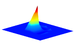
(a) $\phi_{0}$

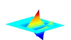
(b) $\psi_{1}^{0}$

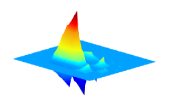
(c) $\psi_{2}^{0}$

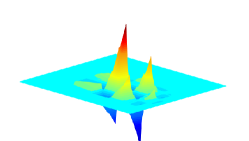
(d) $\psi_{3}^{0}$

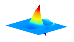
(e) $\psi_{4}^{0}$

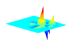
(f) $\psi_{5}^{0}$

Figure 1: Limit functions related to the scaling matrix $\Xi_{0}$ in (22).

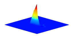
(a) $\phi_{1}$

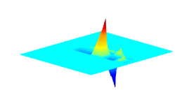
(b) $\psi_{1}^{1}$

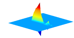
(c) $\psi_{2}^{1}$

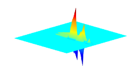
(d) $\psi_{3}^{1}$

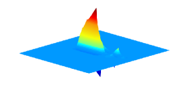
(e) $\psi_{4}^{1}$

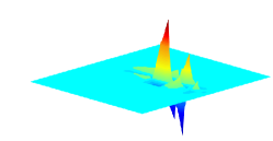
(f) $\psi_{5}^{1}$

Figure 2: Limit functions related to the scaling matrix $\Xi_{1}$ in (22).

Here we consider a bivariate example of matrices of the form (15),

$$\Xi_{0}=\begin{pmatrix}3&0\\ 0&2\end{pmatrix},\qquad\Xi_{1}=\begin{pmatrix}3&-1\\ 0&2\end{pmatrix},$$ (22)

that have minimum determinant possible ($\det\Xi_{0}=6$) because $\sigma_{1}=3$ and $\sigma_{2}=2$. The matrix $\Xi_{1}$ is similar to $\Xi_{0}$, in fact, its Smith factorization is

$$\Xi_{1}=\Gamma_{1}^{-1}\Xi_{0}\Gamma_{1}=\begin{pmatrix}1&1\\ 0&1\end{pmatrix}\begin{pmatrix}3&0\\ 0&2\end{pmatrix}\begin{pmatrix}1&-1\\ 0&1\end{pmatrix}.$$

By (18) the proposed family is jointly contractive and it satisfies the slope resolution property, due to Theorem 6.2.

To define an MMRA with this family of dilation matrices, we follow the construction of orthogonal filters described by (7) and (8). For $\sigma_{1}=3$, we take from [13] the univariate ternary QMF filters

$$g_{1}^{0} =\left(\frac{3+\sqrt{57}}{18},\frac{9+\sqrt{57}}{18},\frac{15+\sqrt{57}}{18},\frac{15-\sqrt{57}}{18},\frac{9-\sqrt{57}}{18},\frac{3-\sqrt{57}}{18}\right),$$

$$g_{1}^{1} =\left(-\frac{\sqrt{2}}{2},\sqrt{2},-\frac{\sqrt{2}}{2},0,0,0\right),$$

$$g_{1}^{2} =\frac{\sqrt{11-\sqrt{57}}}{144}\left(-21+\sqrt{57},-6-2\sqrt{57},9-5\sqrt{57},48+8\sqrt{57},6+2\sqrt{57},-36-4\sqrt{57}\right).$$

For $\sigma_{2}=2$, on the other hand, we choose the univariate QMF Daubechies filters of order $2$

$$g_{2}^{0} =\left(\frac{1+\sqrt{3}}{4},\frac{3+\sqrt{3}}{4},\frac{3-\sqrt{3}}{4},\frac{1-\sqrt{3}}{4}\right),$$

$$g_{2}^{1} =\left(\frac{1-\sqrt{3}}{4},\frac{-3+\sqrt{3}}{4},\frac{3+\sqrt{3}}{4},\frac{-1-\sqrt{3}}{4}\right).$$

The QMF filter system $B_{0}=(b_{\eta}^{0},\,\eta\in\mathbb{Z}_{6})$ with respect to the diagonal matrix $\Xi_{0}$ is composed by the tensor products

$$g_{1}^{k}\otimes g_{2}^{\ell},\qquad k=0,1,2\quad\ell=0,1.$$

In such way, we have one low–pass filter $b_{0}^{0}$ and 5 high–pass filters $b_{i}^{0},\;i=1,\ldots,5$,

$$\begin{array}[]{cc}b_{0}^{0}=g_{1}^{0}\otimes g_{2}^{0},&b_{3}^{0}=g_{1}^{1}\otimes g_{2}^{1},\\ b_{1}^{0}=g_{1}^{0}\otimes g_{2}^{1},&b_{4}^{0}=g_{1}^{2}\otimes g_{2}^{0},\\ b_{2}^{0}=g_{1}^{1}\otimes g_{2}^{0},&b_{5}^{0}=g_{1}^{2}\otimes g_{2}^{1}.\end{array}$$ (23)

From this family of filters we deduce the filters $B_{1}=(b_{\eta}^{1},\,\eta\in\mathbb{Z}_{6})$ associated to $\Xi_{1}$,

$$b_{i}^{1}(\cdot)=b_{i}^{0}(\Gamma_{1}\cdot),\qquad i=0,\ldots,5.$$

By Theorem 5.4 it is possible to define an orthogonal MMRA with dilation matrices $\Xi_{0}$ and $\Xi_{1}$. We denote with

$$\phi_{j}:=\lim_{r\to\infty}S^{r}_{\Xi_{j},b_{0}^{j}}\,\delta,\qquad j\in\mathbb{Z}_{2},$$

the scaling functions and with

$$\psi_{i}^{j}:=\lim_{r\to\infty}S^{r}_{\Xi_{j},b_{0}^{j}}\,b_{i}^{j},\qquad j\in\mathbb{Z}_{2},\;i\in\mathbb{Z}^{+}_{6},$$

the wavelets functions for the prescribed family of matrices (22). Figures 1 and 2 depict the scaling $\phi_{j}$, $j\in\mathbb{Z}_{2}$, and wavelet functions, $\psi_{k}^{j}$, $k\in\mathbb{Z}_{6}^{+}$, with dilation matrices $\Xi_{0}$ and $\Xi_{1}$, respectively.

References

References

[1]
H.-J. Park, A computational theory of Laurent polynomial rings and
multidimensional FIR systems, Ph.D. thesis, University of California at
Berkeley (1995).
[2]
H. Park, C. Woodburn, An algorithmic proof of Suslin’s stability theorem for
polynomial rings, J. Algebra 178 (1995) 277–298.
[3]
M. Cotronei, D. Ghisi, M. Rossini, T. Sauer, An anisotropic directional
subdivision and multiresolution, Advances Comput. Math. 41 (2015) 709–726.
[4]
G. Kutyniok, T. Sauer, Adaptive directional subdivision schemes and shearlet
multiresolution analysis, SIAM J. Math. Anal. 41 (2009) 1436–1471.
[5]
S. Mallat, A Wavelet Tour of Signal Processing: The Sparse Way, 3rd Edition,
Academic Press, 2009.
[6]
W. Dahmen, C. A. Micchelli, Biorthogonal wavelet expansion, Constr. Approx. 13
(1997) 294–328.
[8]
C. A. Micchelli, T. Sauer, Regularity of multiwavelets, Advances Comput. Math.
7 (4) (1997) 455–545.
[9]
M. Vetterli, J. Kovačević, Wavelets and Subband Coding, Prentice Hall,
1995.
[10]
M. Marcus, H. Minc, A Survey of Matrix Theory and Matrix Inequalities, Prindle,
Weber & Schmidt, 1969, paperback reprint, Dover Publications, 1992.
[11]
M. Bozzini, M. Rossini, T. Sauer, E. Volontè, Anisotropic scaling matrices
and subdivision schemes ArXiv:1801.03123.
[12]
C. A. Micchelli, T. Sauer, On vector subdivision, Math. Z. 229 (1998) 621–674.
[13]
C. K. Chui, J. Lian, Construction of compactly supported symmetric and
antisymmetric orthonormal wavelets with scale , Appl. Comput. Harmon.
Anal. 2 (1995) 21–51.
[14]
P. Heller, Rank wavelets with vanishing moments, SIAM J. Matrix Anal.
16 (1995) 502–518.
[15]
T. Sauer, Shearlet multiresolution and multiple refinement, in: G. Kutyniok,
L. D. (Eds.), Shearlets, Springer, 2011.
[16]
T. Sauer, Multiple subdivision, in: J.-D. B. et al. (Ed.), Curves and Surfaces
2011, no. 6920 in Lecture Notes in Computer Science, Springer, 2011, pp.
612–628.
[17]
J. E. Hutchinson, Fractals and self similarity, Indiana Univ. Math. J. 30
(1981) 713–747.