Trade-off Between Work and Correlations in Quantum Thermodynamics

Abstract

Quantum thermodynamics and quantum information are two frameworks for employing quantum mechanical systems for practical tasks, exploiting genuine quantum features to obtain advantages with respect to classical implementations. While appearing disconnected at first, the main resources of these frameworks, work and correlations, have a complicated yet interesting relationship that we examine here. We review the role of correlations in quantum thermodynamics, with a particular focus on the conversion of work into correlations. We provide new insights into the fundamental work cost of correlations and the existence of optimally correlating unitaries, and discuss relevant open problems.

I Introduction

From its inception, classical thermodynamics has been a practically minded theory, aiming to quantify the usefulness and capabilities of machines in terms of performing work. One of the distinguishing features of quantum thermodynamics with respect to classical thermodynamics (and standard quantum statistics) is the level of control that one assumes to have over the degrees of freedom of microscopic (and mesoscopic) quantum systems. This control allows one to identify genuine quantum behaviour in thermodynamics beyond contributions via statistical deviations, e.g., due to the indistinguishability of bosons and fermions. Moreover, this control permits us to consider individual quantum systems as the figurative gears of a quantum machine —quantum “cogwheels” that can be used to extract or store work, which act as catalysts, or mediate interactions. The operating principle of such a (quantum) machine is to use the control over the system to convert one kind of resource into another, for instance, thermal energy into mechanical work. Quantum thermodynamics can hence be viewed as a resource theory Brandão et al. (2013), where energy is a resource, while systems in thermal equilibrium with the environment are considered to be freely available. The control over the system then determines how energy can be spent to manipulate (thermal) quantum states.

At the same time, the manipulation of well-controlled quantum systems is the basic premise for quantum information processing Nielsen and Chuang . The latter, in turn, can also be understood as a resource theory with respect to (quantum) correlations Horodecki and Oppenheim (2013); Eltschka and Siewert (2014). However, it is clear that for any practical application, that this abstract information-theoretic construct must be embedded within a physical context, e.g., such as that provided by quantum thermodynamics. It therefore seems natural to wonder, how the resources of quantum thermodynamics and quantum information theory are related, how they can be converted into each other, and what role resources of one theory play in the other, respectively.

Here, we want to discuss these questions and review the role of (quantum) correlations in quantum thermodynamics (see Refs. Goold et al. (2016); Millen and Xuereb (2016); Vinjanampathy and Anders (2016) for recent reviews). In Section II, we briefly review a few key areas within quantum thermodynamics where (quantum) correlations are of significance, starting with an overview of the basic concepts and definitions in Sections II.A.1 and II.A.2. In Sections II.A.3 and II.B, the consequences of the presence of correlations for the formulation of thermodynamic laws and for the task of work extraction are discussed, respectively.

In Section III, we then focus on the specific question of converting the resource of quantum thermodynamics, i.e., energy, into the resource of quantum information, i.e., correlations. To this end, we first review previous key results Huber et al. (2015); Bruschi et al. (2015); Giorgi and Campbell (2015); Friis et al. (2016); Francica et al. (2017) that provide bounds on the performance of this resource conversion, before turning to a, thus far, unresolved problem: the question of the existence of optimally correlating unitaries. We show that such operations do not always exist and analyse the implications of this observation. Finally, we discuss pertinent open problems in understanding the role of correlations in thermodynamics.

II Correlations in Quantum Thermodynamics

II.A Framework

II.A.1 Quantum thermodynamics in a nutshell

In the following, we consider pairs of quantum mechanical systems that may share correlations. In the context of thermodynamics, these might be, e.g., a system (working body) and a heat bath. In quantum mechanics, these systems are encoded into a bipartite Hilbert space $\mathcal{H}_{\raisebox{0.0pt}{\tiny{$AB$}}}=\mathcal{H}_{\raisebox{0.0pt}{\tiny{$A$}}}\otimes\mathcal{H}_{\raisebox{0.0pt}{\tiny{$B$}}}$, where the tensor factors represent the two subsystems, $A$ and $B$. States describing the joint system are given by density operators $\rho_{\raisebox{0.0pt}{\tiny{$AB$}}}\in\mathcal{L}(\mathcal{H}_{\raisebox{0.0pt}{\tiny{$AB$}}})$, i.e., positive-semidefinite ($\rho_{\raisebox{0.0pt}{\tiny{$AB$}}}\geq 0$), linear operators over $\mathcal{H}_{\raisebox{0.0pt}{\tiny{$AB$}}}$ that satisfy $\textnormal{Tr}(\rho_{\raisebox{0.0pt}{\tiny{$AB$}}})=1$. The energy of the system is further determined by the Hamiltonian $H_{\raisebox{0.0pt}{\tiny{$AB$}}}$, i.e., a self-adjoint operator over $\mathcal{H}_{\raisebox{0.0pt}{\tiny{$AB$}}}$ usually assumed to be bounded from below. Besides the average (internal) energy $E(\rho_{\raisebox{0.0pt}{\tiny{$AB$}}})=\textnormal{Tr}(H\rho_{\raisebox{0.0pt}{\tiny{$AB$}}})$ of the joint system, other state functions central to quantum thermodynamics are the von Neumann entropy $S(\rho_{\raisebox{0.0pt}{\tiny{$AB$}}})=-\textnormal{Tr}\bigl{(}\rho_{\raisebox{0.0pt}{\tiny{$AB$}}}\ln(\rho_{\raisebox{0.0pt}{\tiny{$AB$}}})\bigr{)}$ and the free energy $F(\rho_{\raisebox{0.0pt}{\tiny{$AB$}}})=E(\rho_{\raisebox{0.0pt}{\tiny{$AB$}}})-TS(\rho_{\raisebox{0.0pt}{\tiny{$AB$}}})$, as well as the analogous quantities for the reduced states $\rho_{\raisebox{0.0pt}{\tiny{$A$}}}=\textnormal{Tr}_{\raisebox{0.0pt}{\tiny{$B$}}}(\rho_{\raisebox{0.0pt}{\tiny{$AB$}}})$ and $\rho_{\raisebox{0.0pt}{\tiny{$B$}}}=\textnormal{Tr}_{\raisebox{0.0pt}{\tiny{$A$}}}(\rho_{\raisebox{0.0pt}{\tiny{$AB$}}})$ of the subsystems.

The focus of quantum thermodynamics then lies on the study of the (possible) evolution of $\rho_{\raisebox{0.0pt}{\tiny{$AB$}}}$ and the subsystem states $\rho_{\raisebox{0.0pt}{\tiny{$A$}}}=\textnormal{Tr}_{\raisebox{0.0pt}{\tiny{$B$}}}(\rho_{\raisebox{0.0pt}{\tiny{$AB$}}})$ and $\rho_{\raisebox{0.0pt}{\tiny{$B$}}}=\textnormal{Tr}_{\raisebox{0.0pt}{\tiny{$A$}}}(\rho_{\raisebox{0.0pt}{\tiny{$AB$}}})$ subject to certain constraints on the allowed transformations of the joint system, such as, for example:

1. Conservation of (total) energy of $A$ and $B$:

   $$\rho_{\raisebox{0.0pt}{\tiny{$AB$}}}\mapsto\sigma_{\raisebox{0.0pt}{\tiny{$AB$}}}:\textnormal{Tr}(H_{\raisebox{0.0pt}{\tiny{$AB$}}}\rho_{\raisebox{0.0pt}{\tiny{$AB$}}})=\textnormal{Tr}(H_{\raisebox{0.0pt}{\tiny{$AB$}}}\sigma_{\raisebox{0.0pt}{\tiny{$AB$}}})$$

2. Closed system dynamics:

   $$\rho_{\raisebox{0.0pt}{\tiny{$AB$}}}\mapsto U_{\raisebox{0.0pt}{\tiny{$AB$}}}\rho_{\raisebox{0.0pt}{\tiny{$AB$}}}U^{\dagger}_{\raisebox{0.0pt}{\tiny{$AB$}}}$$

   for some global unitary transformation $U_{\raisebox{0.0pt}{\tiny{$AB$}}}$.

To state its basic laws, then, a first main goal of quantum thermodynamics is to provide meaningful definitions of heat $\Delta Q$ and work $\Delta W$ exchanged between the subsystems. These quantities are not just functions of the state, but depend on the concrete transformations that are applied. In particular, suitable definitions are usually chosen such that the first law of thermodynamics holds for closed joint systems, i.e.,

$$\Delta E =\,\Delta Q+\Delta W\,,$$ (1)

with $\Delta E=E(\rho_{\raisebox{0.0pt}{\tiny{$A$}}}(t+\Delta t))-E(\rho_{\raisebox{0.0pt}{\tiny{$A$}}}(t))$. For this purpose a quantifier often used for the information change within the subsystems is the relative entropy $S(\rho_{\raisebox{0.0pt}{\tiny{$A$}}}(t+\Delta t)\|\rho_{\raisebox{0.0pt}{\tiny{$A$}}}(t))$ of $\rho_{\raisebox{0.0pt}{\tiny{$A$}}}(t+\Delta t)$ w.r.t. $\rho_{\raisebox{0.0pt}{\tiny{$A$}}}(t)$. For arbitrary states $\rho$ and $\sigma$ it is defined as

$$S(\sigma\|\rho) =\,-S(\sigma)-\textnormal{Tr}\bigl{(}\sigma\ln(\rho)\bigr{)}\,.$$ (2)

The relative entropy is nonnegative, $S(\sigma\|\rho)\geq 0$, for all pairs $\rho$ and $\sigma$, with equality iff $\rho=\sigma$ (see, e.g., Vedral (2002) for details), and coincides with the free energy difference $S(\sigma\|\rho)=F(\sigma)-F(\rho)$, whenever $\rho=\tau(\beta)$ is thermal. That is, given a Hamiltonian $H_{\raisebox{0.0pt}{\tiny{$AB$}}}$, the corresponding thermal state is defined as

$$\tau_{\raisebox{0.0pt}{\tiny{$AB$}}}(\beta) =\,\mathcal{Z}^{-1}e^{-\beta H_{\raisebox{0.0pt}{\tiny{$AB$}}}}\,,$$ (3)

where $\beta=1/T$ denotes the inverse temperature and $\mathcal{Z}=\textnormal{Tr}(e^{-\beta H_{\raisebox{0.0pt}{\tiny{$AB$}}}})$ is called the partition function. The above thermal state $\tau_{\raisebox{0.0pt}{\tiny{$AB$}}}(\beta)$ can be considered as the state of the joint system of $A$ and $B$ at thermal equilibrium with an external heat bath at temperature $T$, and represents the maximum entropy state for fixed (internal) energy Jaynes (1957). The relative entropy can hence be understood as measure of distance from thermal equilibrium of the total system.

II.A.2 Quantifying correlations

The properties of equilibrium states strongly depend on the system Hamiltonian. For instance, the joint thermal state $\tau_{AB}$ of systems $A$ and $B$ is completely uncorrelated whenever they are noninteracting, i.e., when $H_{\raisebox{0.0pt}{\tiny{$AB$}}}=H_{\raisebox{0.0pt}{\tiny{$A$}}}+H_{\raisebox{0.0pt}{\tiny{$B$}}}$, where $H_{\raisebox{0.0pt}{\tiny{$A$}}}$ and $H_{\raisebox{0.0pt}{\tiny{$B$}}}$ act nontrivially only on $\mathcal{H}_{\raisebox{0.0pt}{\tiny{$A$}}}$ and $\mathcal{H}_{\raisebox{0.0pt}{\tiny{$B$}}}$, respectively. In this case $\tau_{\raisebox{0.0pt}{\tiny{$AB$}}}$ is a product state $\tau_{\raisebox{0.0pt}{\tiny{$AB$}}}(\beta)=\tau_{\raisebox{0.0pt}{\tiny{$A$}}}(\beta)\otimes\tau_{\raisebox{0.0pt}{\tiny{$B$}}}(\beta)$, where $\tau_{\raisebox{0.0pt}{\tiny{$A$}}}$ and $\tau_{\raisebox{0.0pt}{\tiny{$B$}}}$ are thermal states at the same temperature $T=1/\beta$ w.r.t. the local Hamiltonians $H_{\raisebox{0.0pt}{\tiny{$A$}}}$ and $H_{\raisebox{0.0pt}{\tiny{$B$}}}$, respectively. Conversely, in an interacting system the global state $\rho_{\raisebox{0.0pt}{\tiny{$AB$}}}$ will typically be correlated, and may even be entangled, meaning that the state cannot be decomposed into a mixture of uncorrelated states (see, e.g., Friis et al. (2016) for a discussion).

Such correlations can be quantified in terms of the mutual information

$$\mathcal{I}(\rho_{\raisebox{0.0pt}{\tiny{$AB$}}}) =S(\rho_{\raisebox{0.0pt}{\tiny{$A$}}})+S(\rho_{\raisebox{0.0pt}{\tiny{$B$}}})-S(\rho_{\raisebox{0.0pt}{\tiny{$AB$}}}).$$ (4)

That is, $\mathcal{I}$ quantifies the amount of information about the system that is available globally but not locally. Here, it is important to note $\mathcal{I}$ captures both classical and genuine quantum correlations in the sense that nonzero values of $\mathcal{I}$ may originate in either type of correlation. Nonetheless, it should be noted that any state $\rho_{\raisebox{0.0pt}{\tiny{$AB$}}}$ for which $\mathcal{I}(\rho_{\raisebox{0.0pt}{\tiny{$AB$}}})>S(\rho_{\raisebox{0.0pt}{\tiny{$A$}}})$ or $\mathcal{I}(\rho_{\raisebox{0.0pt}{\tiny{$AB$}}})>S(\rho_{\raisebox{0.0pt}{\tiny{$B$}}})$ features a negative conditional entropy $S(A\|B)=S(\rho_{\raisebox{0.0pt}{\tiny{$A$}}})-\mathcal{I}(\rho_{\raisebox{0.0pt}{\tiny{$AB$}}})$, and is hence Cerf and Adami (1999); Del Rio et al. (2011) necessarily entangled to some extent.

II.A.3 Role of correlations for thermodynamic laws

Indeed, correlations are already central to the foundations of quantum thermodynamics. This manifests in the fundamental difference between describing thermodynamic systems as being composed of isolated parts, or as interacting with each other. When subsystems are considered to be completely isolated, just as in classical thermodynamics, this translates to the quantum mechanical notion of a product state $\rho_{\raisebox{0.0pt}{\tiny{$A$}}}\otimes\rho_{\raisebox{0.0pt}{\tiny{$B$}}}$. However, there are continuing efforts to expand and even challenge this seemingly basic assumption. This includes, e.g., approaches where subsystems (and hence potential correlations between them) are defined using thermodynamic principles Stokes et al. (2017), or those where work and heat exchange in interacting systems is defined in terms of effective local Hamiltonians that depend on correlations Weimer et al. (2008); Teifel and Mahler (2011). In other approaches, the traditional setting of a system separable from its surrounding thermal bath can be extended to a state $\rho_{\raisebox{0.0pt}{\tiny{$AB$}}}$ with correlations between system and bath Partovi (2008); Jennings and Rudolph (2010); Jevtic et al. (2012a, b); Brandão et al. (2015); Alipour et al. (2016); Nath Bera et al. (2017); Müller (2018). This leads to reformulations of the concepts of heat and work and modifications of the classical laws of thermodynamics via the introduction of correlated baths.

In particular, the second law deserves a special mention in this respect. Loosely speaking, it states that the entropy of a subsystem cannot decrease after a thermodynamical transformation, i.e., $\Delta S=S(\rho_{\raisebox{0.0pt}{\tiny{$A$}}}(t+\Delta t))-S(\rho_{\raisebox{0.0pt}{\tiny{$A$}}}(t))\geq 0$, an observation that lies at the heart of the emergence of the so-called thermodynamical arrow of time. However, several authors, have observed how such a relation does not hold true anymore when system and bath are allowed to be initially correlated Partovi (2008); Jennings and Rudolph (2010). This insight can even be traced back to Boltzmann himself Boltzmann (1970, 1897), who, while introducing the so-called Stosszahlansatz (i.e., the assumption of molecular chaos), noticed that in order for the second law of thermodynamics to emerge it was necessary to assume a weakly correlated (cosmological) environment.

Formally speaking, the basic argument showing the intimate connection of correlations with the thermodynamical arrow of time works as follows in its extremal version Partovi (2008); Jennings and Rudolph (2010); Jevtic et al. (2012a, b). Consider a system and bath with local Hamiltonians $H_{\raisebox{0.0pt}{\tiny{$A$}}}$ and $H_{\raisebox{0.0pt}{\tiny{$B$}}}$, such that $H_{\raisebox{0.0pt}{\tiny{$A$}}}\left|\right.\!{n}\!\left.\right\rangle_{\raisebox{0.0pt}{\tiny{$A$}}}=E_{n}^{\raisebox{0.0pt}{\tiny{$A$}}}\left|\right.\!{n}\!\left.\right\rangle_{\raisebox{0.0pt}{\tiny{$A$}}}$ and $H_{\raisebox{0.0pt}{\tiny{$B$}}}\left|\right.\!{n}\!\left.\right\rangle_{\raisebox{0.0pt}{\tiny{$B$}}}=E_{n}^{\raisebox{0.0pt}{\tiny{$B$}}}\left|\right.\!{n}\!\left.\right\rangle_{\raisebox{0.0pt}{\tiny{$B$}}}$. Suppose that there exist constants $\mu_{\raisebox{0.0pt}{\tiny{$A$}}}$ and $\mu_{\raisebox{0.0pt}{\tiny{$B$}}}$ such that the local energy levels $E_{n}^{\raisebox{0.0pt}{\tiny{$A$}}}$ and $E_{n}^{\raisebox{0.0pt}{\tiny{$B$}}}$ satisfy $\mu_{\raisebox{0.0pt}{\tiny{$A$}}}E_{n}^{\raisebox{0.0pt}{\tiny{$A$}}}=\mu_{\raisebox{0.0pt}{\tiny{$B$}}}E_{n}^{\raisebox{0.0pt}{\tiny{$B$}}}=\epsilon_{n}$ for all $n$. Let us further assume that initially system and bath are jointly very close to a (pure) highly entangled state

$$\left|\right.\!{\psi}\!\left.\right\rangle_{\raisebox{0.0pt}{\tiny{$AB$}}} =\,\mathcal{Z}^{-1/2}\sum_{n}\exp(-\gamma\epsilon_{n}/2)\left|\right.\!{n,n}\!\left.\right\rangle_{\raisebox{0.0pt}{\tiny{$AB$}}}\,,$$ (5)

which can be thought of as a thermal state of a suitable interacting Hamiltonian $H_{\raisebox{0.0pt}{\tiny{$AB$}}}$ for very low temperatures (i.e., in the limit $\beta\rightarrow\infty$). The two marginal states $\rho_{\raisebox{0.0pt}{\tiny{$A$}}}$ and $\rho_{\raisebox{0.0pt}{\tiny{$B$}}}$ are thermal w.r.t. $H_{\raisebox{0.0pt}{\tiny{$A$}}}$ and $H_{\raisebox{0.0pt}{\tiny{$B$}}}$ at (different) inverse temperatures $\beta_{\raisebox{0.0pt}{\tiny{$A$}}}=\mu_{\raisebox{0.0pt}{\tiny{$A$}}}\gamma$ and $\beta_{\raisebox{0.0pt}{\tiny{$B$}}}=\mu_{\raisebox{0.0pt}{\tiny{$B$}}}\gamma$ respectively, but with the same entropy $S(\rho_{\raisebox{0.0pt}{\tiny{$A$}}})=S(\rho_{\raisebox{0.0pt}{\tiny{$B$}}})$ since $\rho_{\raisebox{0.0pt}{\tiny{$A$}}}$ and $\rho_{\raisebox{0.0pt}{\tiny{$B$}}}$ have the same spectrum. Suppose now that the two subsystems interact through a global unitary transformation that allows some exchange of energy between the subsystems. Further, let us assume that, w.r.t. to a suitable definition of $Q$ [see the discussion surrounding Eq. (1)], this exchange is interpreted simply as a heat exchange, meaning that the local changes of internal energy satisfy $\Delta E_{\raisebox{0.0pt}{\tiny{$A$}}}=\Delta Q_{\raisebox{0.0pt}{\tiny{$A$}}}$ and $\Delta E_{\raisebox{0.0pt}{\tiny{$B$}}}=\Delta Q_{\raisebox{0.0pt}{\tiny{$B$}}}$, respectively. Since the marginals are initially thermal, we have $\Delta F_{\raisebox{0.0pt}{\tiny{$A$}}}=\Delta E_{\raisebox{0.0pt}{\tiny{$A$}}}-T_{\raisebox{0.0pt}{\tiny{$A$}}}\Delta S_{\raisebox{0.0pt}{\tiny{$A$}}}\geq 0$ and $\Delta F_{\raisebox{0.0pt}{\tiny{$B$}}}=\Delta E_{\raisebox{0.0pt}{\tiny{$B$}}}-T_{\raisebox{0.0pt}{\tiny{$B$}}}\Delta S_{\raisebox{0.0pt}{\tiny{$B$}}}\geq 0$, which leads to $\beta_{\raisebox{0.0pt}{\tiny{$A$}}}\Delta Q_{\raisebox{0.0pt}{\tiny{$A$}}}\geq\Delta S_{\raisebox{0.0pt}{\tiny{$A$}}}$ and $\beta_{\raisebox{0.0pt}{\tiny{$B$}}}\Delta Q_{\raisebox{0.0pt}{\tiny{$B$}}}\geq\Delta S_{\raisebox{0.0pt}{\tiny{$B$}}}$, while $\Delta Q_{\raisebox{0.0pt}{\tiny{$A$}}}+\Delta Q_{\raisebox{0.0pt}{\tiny{$B$}}}=0$. Globally, the constraint on heat exchanges implies

$$\beta_{\raisebox{0.0pt}{\tiny{$A$}}}\Delta Q_{\raisebox{0.0pt}{\tiny{$A$}}}+\beta_{\raisebox{0.0pt}{\tiny{$B$}}}\Delta Q_{\raisebox{0.0pt}{\tiny{$B$}}} \geq\,\Delta\mathcal{I}_{\raisebox{0.0pt}{\tiny{$AB$}}}\,,$$ (6)

where $\Delta\mathcal{I}_{\raisebox{0.0pt}{\tiny{$AB$}}}=\Delta S_{\raisebox{0.0pt}{\tiny{$A$}}}+\Delta S_{\raisebox{0.0pt}{\tiny{$B$}}}$ is the change in the mutual information after the transformation since the unitary leaves the overall entropy invariant. The crucial observation is then that for the above global state $\left|\right.\!{\psi}\!\left.\right\rangle_{\raisebox{0.0pt}{\tiny{$AB$}}}$ the mutual information can be very high initially and can decrease during the transformation such that $\Delta\mathcal{I}_{\raisebox{0.0pt}{\tiny{$AB$}}}<0$. Heat may thus be allowed to flow from the cold to the hot subsystem (e.g., $\Delta Q_{\raisebox{0.0pt}{\tiny{$A$}}}\geq 0$ for $\beta_{\raisebox{0.0pt}{\tiny{$A$}}}\leq\beta_{\raisebox{0.0pt}{\tiny{$B$}}}$). Correlations can thus lead to an anomalous heat flow, see also Levy and Gelbwaser-Klimovsky (2019). Moreover, since the above global state remains pure, the marginals have the same spectra, and we have $\Delta S_{\raisebox{0.0pt}{\tiny{$A$}}}=\Delta S_{\raisebox{0.0pt}{\tiny{$B$}}}$. Therefore, an anomalous heat flow implies a violation of the classical second law of thermodynamics, $\Delta\mathcal{I}_{\raisebox{0.0pt}{\tiny{$AB$}}}<0\ \Rightarrow\ \Delta S_{\raisebox{0.0pt}{\tiny{$A$}}}=\Delta S_{\raisebox{0.0pt}{\tiny{$B$}}}<0$, i.e., the local entropies both decrease, reversing the direction of the thermodynamical arrow of time.

Following this observation, several authors, adopting an information theoretic perspective, have investigated the possibility to generalize the thermodynamic laws in the presence of initial correlations between system and bath, see, e.g., Refs. del Rio et al. (2016); Brandão et al. (2015); Alipour et al. (2016); Nath Bera et al. (2017); Müller (2018). Furthermore, experiments are now being performed for quantum mechanical systems realized in several platforms to observe violations of classical laws of thermodynamics, especially regarding the inversion of the thermodynamic arrow of time Micadei et al. (2017).

Correlations therefore need to be carefully incorporated into the formulation of quantum thermodynamics. However, correlations are not only a source of seemingly paradoxical situations but can also have direct practical relevance for paradigmatic tasks in quantum thermodynamics, as we will discuss in Section II.B, before we analyse what quantum thermodynamics tells us about the work cost and level of control necessary to create correlations in Section III.

II.B Extracting work from correlations

II.B.1 Work extraction using cyclic transformations

A basic but crucial application of thermodynamics is to quantify how much work can be extracted from a given machine operating under a cycle of transformations. In this context, one may consider subsystem $A$ to be a quantum machine that is controlled by the external subsystem $B$. As a general model of such a machine one usually considers an ensemble of, say, $N$ quantum mechanical units, i.e., subsystem $A$ has a Hilbert space $\mathcal{H}_{\raisebox{0.0pt}{\tiny{$A$}}}=\mathcal{H}^{\otimes N}$ with a given (free) Hamiltonian $H_{\raisebox{0.0pt}{\tiny{$A$}}}$. This allows statements about the scaling of the quantum machine’s efficiency and eventual gain (e.g., originating from the ability to create correlations) with $N$ as compared to analogous classical machines.

The external control is usually modelled as a switchable time-dependent (and cyclic) Hamiltonian $H(t)$, such that $H(0)=H(t_{\rm cycle})$ where $t_{\rm cycle}$ is the time of a whole cycle. The following question then arises naturally: Can correlations between the $N$ units of the machine help in extracting work during a thermodynamical cycle?

More specifically, if we evolve the initial state $\rho_{\raisebox{0.0pt}{\tiny{$A$}}}$ with an externally controlled unitary transformation $U$ and compare the resulting difference in energy we get the quantity

$$\Delta W_{U}=\textnormal{Tr}(\rho_{\raisebox{0.0pt}{\tiny{$A$}}}H_{\raisebox{0.0pt}{\tiny{$A$}}})-\textnormal{Tr}(U\rho_{\raisebox{0.0pt}{\tiny{$A$}}}U^{{\dagger}}H_{\raisebox{0.0pt}{\tiny{$A$}}}).$$ (7)

If positive, it describes the amount of energy that is gained after $U$ and is usually interpreted as extracted work, i.e., the process is assumed to be performed adiabatically with the external control Perarnau-Llobet et al. (2015). Thus, frequently (7) is seen as a figure of merit that should be maximized with respect to the available resources, like the initial state $\rho_{\raisebox{0.0pt}{\tiny{$A$}}}$, the externally controlled evolution $U$ and the free system Hamiltonian $H_{\raisebox{0.0pt}{\tiny{$A$}}}$. Fixing or optimizing over the triple ($\rho_{\raisebox{0.0pt}{\tiny{$A$}}},U,H_{\raisebox{0.0pt}{\tiny{$A$}}}$) allows one to ask questions like: Which combination of resources yields the most work? A frequently studied special case is that of ergotropy Allahverdyan et al. (2004), corresponding to a fixed Hamiltonian and a fixed state while optimizing over all unitaries on $\mathcal{H}_{\raisebox{0.0pt}{\tiny{$A$}}}$, i.e.,

$$\Delta W_{\rm ergotropy}:=\max_{U}\ \Delta W_{U}.$$ (8)

States that do not allow for work extraction with respect to a specified class of operations (typically unitary transformations) are called passive Pusz and Woronowicz (1978).

In other words, for any state $\rho$ the unitary realizing the maximum in Eq. (8) is the one that transforms the state to a corresponding passive state $U\rho\,U^{\dagger}=\rho_{\rm passive}$, and the ergotropy represents the work that is extractable from the system with the specified operations. Quantum systems in passive states thus have a simple practical interpretation as the analogues of empty batteries.

II.B.2 Role of correlations for work extraction

An interesting distinction between the concepts of passive and thermal states that has recently been discovered Alicki and Fannes (2013) is the following. A state is passive if and only if it is diagonal in the energy eigenbasis and its eigenvalues are decreasing with increasing energy. While this is certainly true for thermal states, it can also be the case for many other eigenvalue distributions which are not thermal. In summary, thermality implies passivity, but the converse is not necessarily true.

The special role of thermal states comes to light when considering many copies of the system: While $\tau(\beta)^{\otimes N}$ is still thermal (and thus passive) for any $N$, $\rho_{\mathrm{passive}}^{\otimes N}$ is passive for all $N$ if and only if $\rho_{\mathrm{passive}}$ is a thermal state Lenard (1978); Alicki and Fannes (2013). In other words, thermal states are the only completely passive states. This has interesting consequences when interpreting passive states as empty batteries. While a single battery appears empty, i.e., no work whatsoever can be extracted, it may be the case that adding a second empty battery would enable a correlating global transformation to extract work out of the two empty batteries. This interesting situation is termed work extraction by activation.

This fact leads to a first affirmative answer to the question of whether correlating operations can help for work extraction: Unitary transformations can extract work more efficiently if they are able to generate entanglement. More precisely, a quantitative analysis of the relation between entanglement generation and work extraction Hovhannisyan et al. (2013) shows that the trade-off is more accurately specified as occurring between entangling power and the number of required operations (in other words, time) for work extraction: The less entanglement is generated during the work extraction process, the more time is needed to extract work. However, note that the final state need not be entangled.

The above example of two empty batteries showing the difference between local passivity and (true global) passivity can be employed to construct another enlightening example. In analogy to the batteries above, let us define a state $\rho_{\raisebox{0.0pt}{\tiny{$AB$}}}$ that is locally thermal (thus locally passive) in each marginal, i.e., $\textnormal{Tr}_{\raisebox{0.0pt}{\tiny{$B$}}}(\rho_{\raisebox{0.0pt}{\tiny{$AB$}}})=\tau_{\raisebox{0.0pt}{\tiny{$A$}}}(\beta)$ and $\textnormal{Tr}_{\raisebox{0.0pt}{\tiny{$A$}}}(\rho_{\raisebox{0.0pt}{\tiny{$AB$}}})=\tau_{\raisebox{0.0pt}{\tiny{$B$}}}(\beta)$. Let us now imagine that, contrary to the previous example, the state $\rho_{\raisebox{0.0pt}{\tiny{$AB$}}}$ is correlated. If we can extract work from this state, then it can be argued that all the work must have come from its correlations, since there can be no contributions from local operations (due to the passivity of the marginals) nor from activation, due to the fact that thermal states do not allow for work extraction by activation. An example of such a state is provided in Perarnau-Llobet et al. (2015). For locally thermal states of noninteracting systems all correlations hence imply extractable work.

II.B.3 Role of correlations for work storage

A problem that can be considered dual to the above is how to efficiently charge an initially empty quantum battery (see also Campaioli et al. (2019)). Formally, the problem is to find a suitable way of transforming a state $\rho$ to another state $\sigma=U\rho U^{\dagger}$ such that the latter contains more extractable work, i.e., $\Delta W_{U}\leq 0$ as in Eq. (7). As previously for work extraction, one is primarily interested in charging processes based on cycles of transformations. However, in contrast to the previous problem, one is here not necessarily interested in asking how much work may be stored in principle. Instead other figures of merit become important, indicating certain desirable properties of the charging process or the final state for fixed $\Delta W_{U}$. Examples for such properties include charging power Binder et al. (2015), fluctuations during the charging process or the variance of the final charge Friis and Huber (2018). The key question that we wish to discuss here is: Is it beneficial for work storage to (be able to) generate correlations during the process?

While correlations themselves turn out not to be directly relevant in any crucial way, it appears that the control over correlating transformations can provide significant advantages, even if no actual correlations are created. Specifically, in Ref. Binder et al. (2015) the authors show that the power of charging a battery, defined as $P:=\langle\Delta W_{U}\rangle/\Delta t$, i.e., the ratio of average work $\langle\Delta W_{U}\rangle$ and time $\Delta t$, can be enhanced by allowing entangling global unitaries $U$ on an initially uncorrelated product state $\rho_{1}\otimes\dots\otimes\rho_{N}$. However, whether such entangling operations actually create entanglement during the cycle is irrelevant Campaioli et al. (2017). As is discussed in more detail in Campaioli et al. (2019), the trade-off is rather between entanglement generated during the process and the speed of the process itself. Focussing on the practical aspects of implementing this idea, in Ref. Ferraro et al. (2018) the authors study a non-unitary charging process of a quantum battery of $N$ qubits coupled to a single photonic mode.

II.B.4 Work extraction and storage with restricted control

For understanding fundamental bounds on work extraction and storage correlations are thus of significance, or rather, the ability to create them. This highlights the fact that this ability is linked to the control one has over the system and operations thereon. In particular, maximization such as in Eq. (8) may yield solutions that cannot be practically implemented or whose realization comes at a high cost itself. Therefore, subsequent works have focused on understanding the limitations of work extraction and work storage in terms of more restricted sets of states/operations such as Gaussian states and unitaries Brown et al. (2016); Friis and Huber (2018). This has been motivated also by the easier practical implementation in CV systems such as encountered in quantum optics of Gaussian operations, as opposed to arbitrary unitaries. In particular, this is manifest when considering driven transformations, where Gaussian operations appear as the simplest type of operation according to the hierarchy of driving Hamiltonians, which are at most quadratic in the system’s annihilation and creation operators for Gaussian unitaries.

As we have already emphasized, passivity is defined with respect to an underlying class of state transformations, i.e., unitaries (cyclic Hamiltonian processes). An interesting variant of the problem in Eq. (8) is thus given by the restricted case of Gaussian unitary transformations Brown et al. (2016). This leads to the notion of Gaussian passivity as a special case of passivity in the sense that passivity implies Gaussian passivity, but not vice versa. The role of correlations in such a scenario is particularly interesting. In particular, the authors show that it is always possible to extract work from an entangled Gaussian state via two-mode squeezing operations. For general non-Gaussian states, however, the ability to extract work via (dis)entangling Gaussian unitaries (two-mode squeezing) does not indicate entanglement, and the inability to do so does not imply separability either.

In the complementary problem of battery charging, the subset of Gaussian operations turns out to provide a trade-off between good precision (energy variance) and practical implementability of a battery charging protocol with a fixed target amount of energy $\Delta W$ Friis and Huber (2018). Here, correlations can provide minor advantages in some cases but do not play a conceptually important role.

To conclude this section it is also interesting to point out that, as observed in Ref. Brunelli et al. (2017) the argument that entanglement (or the ability to create it) can provide an advantage in work extraction can also be turned around and exploited to design entanglement certification schemes based on extractable work. In other words, it is possible to witness entanglement by quantifying the extracted work from a thermodynamic cycle, such as the Szilard engine considered in Brunelli et al. (2017). Interestingly, the entanglement criterion based on work extraction becomes necessary and sufficient for two-mode Gaussian states. However, the authors also show that the above scheme cannot be applied for the certification of genuine multipartite entanglement.

III Energy Cost of Creating Correlations

III.A Trade-off between work and correlations

Now that we have an overview of the importance of correlations (and the transformations that can create them) for quantum thermodynamics and its paradigmatic tasks, let us consider the situation from a different perspective. Correlations, in particular, entanglement, are the backbone of quantum information processing. However, if an abstract information theory is to be applied in practice, it requires a physical context, such as is provided by quantum thermodynamics. There, as we have seen above, the freely available equilibrium state of two (noninteracting) systems is uncorrelated. This means that both an investment of energy and a certain level of control (the ability to perform correlating transformations) are required to create the desired correlations.

Thus, formally speaking, one is interested in determining the fundamental limits for the energy cost of creating correlations, where we choose to quantify the latter by the mutual information of Eq. (4) between two quantum systems $A$ and $B$, since the mutual information arises quite naturally in the thermodynamic context. These subsystems are assumed to be initially in a joint thermal state $\tau_{\raisebox{0.0pt}{\tiny{$AB$}}}(\beta)=\tau_{\raisebox{0.0pt}{\tiny{$A$}}}(\beta)\otimes\tau_{\raisebox{0.0pt}{\tiny{$B$}}}(\beta)$ with respect to a noninteracting Hamiltonian $H_{\raisebox{0.0pt}{\tiny{$AB$}}}=H_{\raisebox{0.0pt}{\tiny{$A$}}}+H_{\raisebox{0.0pt}{\tiny{$B$}}}$ at a particular ambient temperature $T=1/\beta$. To correlate $A$ and $B$, it is necessary to move the joint system out of equilibrium, which comes at a nonzero work cost $W$. For instance, when one acts unitarily on the system, this cost can be expressed as $W=\Delta E_{\raisebox{0.0pt}{\tiny{$A$}}}+\Delta E_{\raisebox{0.0pt}{\tiny{$B$}}}$. The question at hand is then: What is the maximal amount of correlation between $A$ and $B$ that can be reached, given a fixed amount of available energy $W$?

Clearly, the answer very much depends on the operations that are allowed, as well as on the energy level structure of the local Hamiltonians. For instance, one may consider applying only global unitary transformations $U_{\raisebox{0.0pt}{\tiny{$AB$}}}$, realized via some external control. If one wishes to optimally convert work into correlations, it is clear that the marginals of the final state must be passive. Otherwise, energy extractable by local unitaries (which leave $\mathcal{I}_{\raisebox{0.0pt}{\tiny{$AB$}}}$ invariant) would be left in the system. Indeed, the marginals must be completely passive (thus thermal), such that no work can be extracted locally from any number of copies. The optimally correlated target state $\rho_{\raisebox{0.0pt}{\tiny{$AB$}}}=U_{\raisebox{0.0pt}{\tiny{$AB$}}}\tau_{\raisebox{0.0pt}{\tiny{$AB$}}}(\beta)U_{\raisebox{0.0pt}{\tiny{$AB$}}}^{\dagger}$ must hence be such that $\rho_{\raisebox{0.0pt}{\tiny{$A$}}}=\textnormal{Tr}_{\raisebox{0.0pt}{\tiny{$B$}}}(\rho_{\raisebox{0.0pt}{\tiny{$AB$}}})=\tau_{\raisebox{0.0pt}{\tiny{$A$}}}(\beta_{\raisebox{0.0pt}{\tiny{$A$}}})$ and $\rho_{\raisebox{0.0pt}{\tiny{$B$}}}=\textnormal{Tr}_{\raisebox{0.0pt}{\tiny{$A$}}}(\rho_{\raisebox{0.0pt}{\tiny{$AB$}}})=\tau_{\raisebox{0.0pt}{\tiny{$B$}}}(\beta_{\raisebox{0.0pt}{\tiny{$B$}}})$. At the same time, one wishes to increase the correlations, i.e., to achieve the maximal amount of mutual information increase $\Delta\mathcal{I}_{\raisebox{0.0pt}{\tiny{$AB$}}}=\Delta S_{\raisebox{0.0pt}{\tiny{$A$}}}+\Delta S_{\raisebox{0.0pt}{\tiny{$B$}}}\geq 0$. At fixed average energy input $\Delta E=E(\tau_{\raisebox{0.0pt}{\tiny{$A$}}}(\beta_{\raisebox{0.0pt}{\tiny{$A$}}}))+E(\tau_{\raisebox{0.0pt}{\tiny{$B$}}}(\beta_{\raisebox{0.0pt}{\tiny{$B$}}}))-E(\tau_{\raisebox{0.0pt}{\tiny{$AB$}}}(\beta))$, the mutual information is then maximized for maximal $S(\tau_{\raisebox{0.0pt}{\tiny{$A$}}}(\beta_{\raisebox{0.0pt}{\tiny{$A$}}}))+S(\tau_{\raisebox{0.0pt}{\tiny{$B$}}}(\beta_{\raisebox{0.0pt}{\tiny{$B$}}}))=S(\tau_{\raisebox{0.0pt}{\tiny{$A$}}}(\beta_{\raisebox{0.0pt}{\tiny{$A$}}})\otimes\tau_{\raisebox{0.0pt}{\tiny{$B$}}}(\beta_{\raisebox{0.0pt}{\tiny{$B$}}}))$. The maximum entropy principle then suggests that the final state marginals should be thermal at the same temperature $\beta_{\raisebox{0.0pt}{\tiny{$A$}}}=\beta_{\raisebox{0.0pt}{\tiny{$B$}}}$. But do unitaries exist that can achieve this?

The above requirements are indeed already quite strong, as we can observe through the following extremal example. Let us imagine that initially the two subsystems are in a pure (ground) state (i.e., the limit $\beta\rightarrow\infty$) $\tau_{\raisebox{0.0pt}{\tiny{$AB$}}}(\beta)=\left|\right.\!{0}\!\left.\right\rangle\!\!\left\langle\right.\!{0}\!\left.\right|_{\raisebox{0.0pt}{\tiny{$A$}}}\otimes\left|\right.\!{0}\!\left.\right\rangle\!\!\left\langle\right.\!{0}\!\left.\right|_{\raisebox{0.0pt}{\tiny{$B$}}}$ at zero initial energy. Then, any unitary will still output a pure state $\left|\right.\!{\psi}\!\left.\right\rangle_{\raisebox{0.0pt}{\tiny{$AB$}}}=U_{\raisebox{0.0pt}{\tiny{$AB$}}}\left|\right.\!{00}\!\left.\right\rangle_{\raisebox{0.0pt}{\tiny{$AB$}}}$, and the requirement of the marginals to be thermal states leads to a state as in Eq. (5), i.e.,

$$\left|\right.\!{\psi}\!\left.\right\rangle_{\raisebox{0.0pt}{\tiny{$AB$}}} =\,\mathcal{Z}^{-1/2}\sum_{n}\lambda_{n}\left|\right.\!{n,n}\!\left.\right\rangle_{\raisebox{0.0pt}{\tiny{$AB$}}}\,,$$ (9)

with $\lambda_{n}^{2}=\exp(-\beta_{\raisebox{0.0pt}{\tiny{$A$}}}E^{\raisebox{0.0pt}{\tiny{$A$}}}_{n})=\exp(-\beta_{\raisebox{0.0pt}{\tiny{$B$}}}E^{\raisebox{0.0pt}{\tiny{$B$}}}_{n})$. The requirement of having a fixed amount of energy available further demands

$$W =\sum_{n}\lambda_{n}^{2}(E^{\raisebox{0.0pt}{\tiny{$A$}}}_{n}+E^{\raisebox{0.0pt}{\tiny{$B$}}}_{n}),$$ (10)

which in general translates into a complicated relation between the two final effective inverse temperatures $\beta_{\raisebox{0.0pt}{\tiny{$A$}}}$ and $\beta_{\raisebox{0.0pt}{\tiny{$B$}}}$.

Thus, further constraints, e.g., on the final temperatures of the marginal states, on the initial Hamiltonians of the two systems, or on the external control available might already lead to an impossibility of achieving such an optimal conversion between work and correlations. In the following we will make this statement more precise, discuss the relevant questions arising in this context, and give some (partial) answers.

III.B Fundamental cost of correlations

With the realization that there is a finite work cost for the creation of correlations in noninteracting systems Huber et al. (2015); Bruschi et al. (2015), or for the increase of correlations in the presence of correlated thermal states for interacting systems Friis et al. (2016), two immediate pertinent questions for the trade-off between the resources work and correlations can be formulated. (i) On the one hand, it is of interest to understand the fundamental limitations on achievable correlations without any restrictions on the complexity of the involved operations or the time these may take. We can thus ask: What is the theoretical minimum work cost for any amount of correlation between two given systems? (ii) On the other hand, it is of course of practical importance to learn what can be achieved under practical conditions, i.e., in finite time and with limited control over the system, that is: What is the minimum work cost of correlations that is practically achievable?

Let us formulate those questions more precisely following the treatment in Bruschi et al. (2015). We first observe that any physical transformation of a system $S$ can be thought of as a unitary map $U_{\raisebox{0.0pt}{\tiny{$SR$}}}$ acting on a larger Hilbert space that includes an external reservoir $R$. In this context one may further assume that $S$ and $R$ are initially not correlated, i.e., that initially we have $\tau_{\raisebox{0.0pt}{\tiny{$SR$}}}(\beta)=\tau_{\raisebox{0.0pt}{\tiny{$S$}}}(\beta)\otimes\tau_{\raisebox{0.0pt}{\tiny{$R$}}}(\beta)$. Then, the work cost to bring such a state out of equilibrium is

$$W =\textnormal{Tr}\Bigl{(}H\bigl{[}\rho_{\raisebox{0.0pt}{\tiny{$SR$}}}-\tau_{\raisebox{0.0pt}{\tiny{$SR$}}}(\beta)\bigr{]}\Bigr{)}=\Delta E_{\raisebox{0.0pt}{\tiny{$S$}}}+\Delta E_{\raisebox{0.0pt}{\tiny{$R$}}},\vspace*{-2mm}$$ (11)

where the overall final state is $\rho_{\raisebox{0.0pt}{\tiny{$SR$}}}=U_{\raisebox{0.0pt}{\tiny{$SR$}}}\hskip 0.5pt\tau_{\raisebox{0.0pt}{\tiny{$SR$}}}(\beta)U_{\raisebox{0.0pt}{\tiny{$SR$}}}^{\dagger}$, and if we further assume that $H=H_{\raisebox{0.0pt}{\tiny{$S$}}}+H_{\raisebox{0.0pt}{\tiny{$R$}}}$, then the energy contributions split up into $\Delta E_{\raisebox{0.0pt}{\tiny{$S$}}}=\textnormal{Tr}\bigl{(}H_{\raisebox{0.0pt}{\tiny{$S$}}}[\rho_{\raisebox{0.0pt}{\tiny{$SR$}}}-\tau_{\raisebox{0.0pt}{\tiny{$SR$}}}(\beta)]\bigr{)}$ and $\Delta E_{\raisebox{0.0pt}{\tiny{$R$}}}=\textnormal{Tr}\bigl{(}H_{\raisebox{0.0pt}{\tiny{$R$}}}[\rho_{\raisebox{0.0pt}{\tiny{$SR$}}}-\tau_{\raisebox{0.0pt}{\tiny{$SR$}}}(\beta)]\bigr{)}$. We note also that similar expressions in related contexts can be found, e.g., in Oppenheim et al. (2002, 2003); Esposito and Van den Broeck (2011); Reeb and Wolf (2014). One may then rewrite Eq. (11) by expressing the internal energy differences via the changes in free energy and entropy and obtain

$$W =\,\Delta F_{\raisebox{0.0pt}{\tiny{$S$}}}+\Delta F_{\raisebox{0.0pt}{\tiny{$R$}}}\,+\,T\,\mathcal{I}_{\raisebox{0.0pt}{\tiny{$SR$}}}\,,$$ (12)

where one makes also use of the fact that the initial thermal state is uncorrelated, $S(\tau_{\raisebox{0.0pt}{\tiny{$SR$}}})=S(\tau_{\raisebox{0.0pt}{\tiny{$S$}}})+S(\tau_{\raisebox{0.0pt}{\tiny{$R$}}})$ and that $U_{\raisebox{0.0pt}{\tiny{$SR$}}}$ leaves the global entropy invariant, i.e., $S(\rho_{\raisebox{0.0pt}{\tiny{$SR$}}})=S(\tau_{\raisebox{0.0pt}{\tiny{$SR$}}})$.

In the above expression, one recognizes the mutual information $\mathcal{I}_{\raisebox{0.0pt}{\tiny{$SR$}}}$ between the system and the reservoir. In complete analogy to the reasoning that leads to Eq. (12), one may further rewrite the free energy change of the system $S$ comprising the subsystems $A$ and $B$ as

$$\Delta F_{\raisebox{0.0pt}{\tiny{$S$}}} =\,\Delta F_{\raisebox{0.0pt}{\tiny{$A$}}}+\Delta F_{\raisebox{0.0pt}{\tiny{$B$}}}\,+\,T\,\mathcal{I}_{\raisebox{0.0pt}{\tiny{$AB$}}}\,.$$ (13)

Combining Eqs. (12) and (13) and noting that the initial states of $A$, $B$ and $R$ are thermal, such that the free energy differences can be expressed via the relative entropy, one thus arrives at

$$\beta W =\,S(\rho_{\raisebox{0.0pt}{\tiny{$R$}}}\|\tau_{\raisebox{0.0pt}{\tiny{$R$}}})+S(\rho_{\raisebox{0.0pt}{\tiny{$A$}}}\|\tau_{\raisebox{0.0pt}{\tiny{$A$}}})+S(\rho_{\raisebox{0.0pt}{\tiny{$B$}}}\|\tau_{\raisebox{0.0pt}{\tiny{$B$}}})+\mathcal{I}_{\raisebox{0.0pt}{\tiny{$SR$}}}+\mathcal{I}_{\raisebox{0.0pt}{\tiny{$AB$}}},$$ (14)

where $\rho_{\raisebox{0.0pt}{\tiny{$A$}}}=\textnormal{Tr}_{\raisebox{0.0pt}{\tiny{$BR$}}}(\rho_{\raisebox{0.0pt}{\tiny{$SR$}}})$, $\rho_{\raisebox{0.0pt}{\tiny{$B$}}}=\textnormal{Tr}_{\raisebox{0.0pt}{\tiny{$AR$}}}(\rho_{\raisebox{0.0pt}{\tiny{$SR$}}})$, and $\rho_{\raisebox{0.0pt}{\tiny{$R$}}}=\textnormal{Tr}_{\raisebox{0.0pt}{\tiny{$AB$}}}(\rho_{\raisebox{0.0pt}{\tiny{$SR$}}})$ are the reduced states after the transformation. Since $S(\rho\|\sigma)\geq 0$ for all $\rho$ and $\sigma$ and $\mathcal{I}_{\raisebox{0.0pt}{\tiny{$SR$}}}\geq 0$ as well, it becomes clear that the fundamental upper bound for the correlations between $A$ and $B$ is

$$\mathcal{I}_{\raisebox{0.0pt}{\tiny{$AB$}}} \leq\beta W.$$ (15)

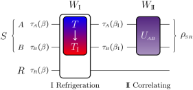
Figure 1: Two-step correlating protocol: The temperature of the initially uncorrelated subsystems $A$ and $B$ forming the system $S$ is first lowered from $T$ to $T_{\mathrm{I}}<T$ using the interaction with the reservoir $R$ at the expense of the work $W_{\mathrm{I}}$. In a second step, the reservoir is decoupled from the system, before $A$ and $B$ are correlated by a unitary $U_{\raisebox{0.0pt}{\tiny{$AB$}}}$, at energy cost $W_{\mathrm{I\!I}}$.

It is then crucial to note that tightness of this bound is only given when $S(\rho_{\raisebox{0.0pt}{\tiny{$R$}}}\|\tau_{\raisebox{0.0pt}{\tiny{$R$}}})=0$ and $\mathcal{I}_{\raisebox{0.0pt}{\tiny{$SR$}}}=0$. On the one hand, these conditions are trivially met when one performs unitary operations acting solely on the system $S$, but not on $R$. We will return to this scenario in Section III.C. On the other hand, one could assume perfect control over an arbitrarily large reservoir $R$, i.e., one that is complex enough to thermalize the system whenever $S$ and $R$ come in contact Åberg (2013) (see also Skrzypczyk et al. (2014) for description of the involved unitaries), such that $R$ can be assumed to be left in its original state with no correlations created between $S$ and $R$.

A protocol that operates based on the latter premise was presented in Bruschi et al. (2015) and consists of two steps to reach the optimal trade-off between work and correlations, i.e., $\mathcal{I}_{\raisebox{0.0pt}{\tiny{$AB$}}}=\beta W$, see Fig. 1. In the first step with work cost $W_{\mathrm{I}}$, the temperature of the system $S$ is lowered from $T$ to $T_{\mathrm{I}}=1/\beta_{\mathrm{I}}<T$. Here one uses the contact to $R$ to refrigerate $S$, resorting to arbitrarily slow processes to do so, such that the cooling cost is given by the free energy difference, $W_{\mathrm{I}}=F\bigl{(}\tau_{\raisebox{0.0pt}{\tiny{$S$}}}(\beta_{\mathrm{I}})\bigr{)}-F\bigl{(}\tau_{\raisebox{0.0pt}{\tiny{$S$}}}(\beta)\bigr{)}$. In the second step, a unitary $U_{\raisebox{0.0pt}{\tiny{$AB$}}}$ acting only on $S$ is used to correlate $A$ and $B$ at work cost $W_{\mathrm{II}}$. It is assumed that $U_{\raisebox{0.0pt}{\tiny{$AB$}}}$ is of such a form that the marginals are returned to locally thermal states at the original temperature $T$. That is, they have to satisfy $\rho_{\raisebox{0.0pt}{\tiny{$A$}}}=\tau_{\raisebox{0.0pt}{\tiny{$A$}}}(\beta)$ and $\rho_{\raisebox{0.0pt}{\tiny{$B$}}}=\tau_{\raisebox{0.0pt}{\tiny{$B$}}}(\beta)$ in order to obtain $S(\rho_{\raisebox{0.0pt}{\tiny{$A$}}}\|\tau_{\raisebox{0.0pt}{\tiny{$A$}}})=S(\rho_{\raisebox{0.0pt}{\tiny{$B$}}}\|\tau_{\raisebox{0.0pt}{\tiny{$B$}}})=0$ in Eq. (14). This last requirement determines the splitting of the work cost $W$ into $W_{\mathrm{I}}$ and $W_{\mathrm{II}}$. One thus finds that there exists a (low-energy) regime, at least in principle, with a linear trade-off between work and correlations, provided that one can exert the mentioned rigorous control over the degrees of freedom of $R$ and that the desired optimal unitaries $U_{\raisebox{0.0pt}{\tiny{$AB$}}}$ exist.

However, even if this is so, there is a threshold input energy, above which the conversion can only occur sublinearly Bruschi et al. (2015). That is, when $\beta W>S\bigl{(}\tau_{\raisebox{0.0pt}{\tiny{$S$}}}(\beta)\bigr{)}$, the conditions above mean that the ground state is reached in the first step of the protocol, and the excess energy is invested into the second step (a situation similar to the example mentioned in the above preliminary discussion). While the protocol is still optimal, one nonetheless has the strict inequality $\mathcal{I}_{\raisebox{0.0pt}{\tiny{$AB$}}}<\beta W$.

III.C Optimally correlating unitaries

However, open questions remain associated to the protocol discussed in the previous section. First, the protocol makes use of the conjectured existence of the unitaries $U_{\raisebox{0.0pt}{\tiny{$AB$}}}$, allowing to reach a final state with $\rho_{\raisebox{0.0pt}{\tiny{$A$}}}=\tau_{\raisebox{0.0pt}{\tiny{$A$}}}(\beta)$ and $\rho_{\raisebox{0.0pt}{\tiny{$B$}}}=\tau_{\raisebox{0.0pt}{\tiny{$B$}}}(\beta)$ starting from $\tau_{\raisebox{0.0pt}{\tiny{$S$}}}(\beta_{\mathrm{I}})$, i.e., with final state marginals that are both effectively at the original temperature. Second, one may question the practicality of the assumptions about the control over $R$ and whether $W_{\mathrm{I}}=F\bigl{(}\tau_{\raisebox{0.0pt}{\tiny{$S$}}}(\beta_{\mathrm{I}})\bigr{)}-F\bigl{(}\tau_{\raisebox{0.0pt}{\tiny{$S$}}}(\beta)\bigr{)}$, $S(\rho_{\raisebox{0.0pt}{\tiny{$R$}}}\|\tau_{\raisebox{0.0pt}{\tiny{$R$}}})=0$ and $\mathcal{I}_{\raisebox{0.0pt}{\tiny{$SR$}}}=0$ may be achieved within reasonable (time) constraints. Both of these issues connect to the previously mentioned scenario where one operates exclusively (and unitarily) on the closed systems $S$. There, the control requirement on $R$ is relaxed from assuming the ability to perform arbitrary unitaries on the overall Hilbert space, to that of isolating and unitarily acting on the significantly smaller system $S$.

Moreover, both situations raise the question whether the respective optimal unitaries exist. In the case of the unitaries $U_{\raisebox{0.0pt}{\tiny{$AB$}}}$ for step $\mathrm{II}$ of the protocol described in the previous section, the special requirement to reach $\mathcal{I}_{\raisebox{0.0pt}{\tiny{$AB$}}}=\beta W$ in the low-energy regime where $\beta W\leq S\bigl{(}\tau_{\raisebox{0.0pt}{\tiny{$S$}}}(\beta)\bigr{)}$, is that the effective temperatures of the marginals of the final state are both the original temperature $T=1/\beta$. Mathematically, we can phrase the question of the existence of $U_{\raisebox{0.0pt}{\tiny{$AB$}}}$ like this:

Question 1.

Does there exist a unitary $U_{\raisebox{0.0pt}{\tiny{$AB$}}}$ on $\mathcal{H}_{\raisebox{0.0pt}{\tiny{$AB$}}}$ such that

$$\rho_{\raisebox{0.0pt}{\tiny{$A$}}} =\textnormal{Tr}_{\raisebox{0.0pt}{\tiny{$B$}}}\bigl{(}U_{\raisebox{0.0pt}{\tiny{$AB$}}}\tau_{\raisebox{0.0pt}{\tiny{$AB$}}}(\beta_{\mathrm{I}})U_{\raisebox{0.0pt}{\tiny{$AB$}}}^{\dagger}\bigr{)}=\tau_{\raisebox{0.0pt}{\tiny{$A$}}}(\beta),$$ (16)

$$\rho_{\raisebox{0.0pt}{\tiny{$B$}}} =\textnormal{Tr}_{\raisebox{0.0pt}{\tiny{$A$}}}\bigl{(}U_{\raisebox{0.0pt}{\tiny{$AB$}}}\tau_{\raisebox{0.0pt}{\tiny{$AB$}}}(\beta_{\mathrm{I}})U_{\raisebox{0.0pt}{\tiny{$AB$}}}^{\dagger}\bigr{)}=\tau_{\raisebox{0.0pt}{\tiny{$B$}}}(\beta),$$ (17)

for every pair of local Hamiltonians $H_{\raisebox{0.0pt}{\tiny{$A$}}}$ and $H_{\raisebox{0.0pt}{\tiny{$B$}}}$, for all temperatures $T_{\mathrm{I}}=1/\beta_{\mathrm{I}}$ (after the step $\mathrm{I}$) and all initial (and thus effective final) temperatures $T=1/\beta\geq T_{\mathrm{I}}$?

For some important special cases, Question 1 can be answered affirmatively. For instance, it was shown in Huber et al. (2015) that such optimally correlating unitaries exist whenever the local Hamiltonians are identical, $H_{\raisebox{0.0pt}{\tiny{$A$}}}=H_{\raisebox{0.0pt}{\tiny{$B$}}}$, and either all energy levels are equally spaced, i.e., and $E_{m+1}-E_{m}=E_{n+1}-E_{n}$ for all $m,n$ such that $H_{\raisebox{0.0pt}{\tiny{$A$}}}\left|\right.\!{n}\!\left.\right\rangle=E_{n}\left|\right.\!{n}\!\left.\right\rangle$, or for arbitrary spacings when the difference between $T_{\mathrm{I}}$ and $T$ is large enough (for a quantitative statement see the appendix of Huber et al. (2015)).

In particular, for two qubits, $\mathcal{H}_{\raisebox{0.0pt}{\tiny{$A$}}}=\mathcal{H}_{\raisebox{0.0pt}{\tiny{$B$}}}=\mathbb{C}^{2}$ this means that optimal generation of correlations in the low-energy regime is always possible as long as $H_{\raisebox{0.0pt}{\tiny{$A$}}}=H_{\raisebox{0.0pt}{\tiny{$B$}}}$, since qubits only posses a single energy gap. However, as the preliminary extremal example treated above in Section III.A suggests, whenever $H_{\raisebox{0.0pt}{\tiny{$A$}}}\neq H_{\raisebox{0.0pt}{\tiny{$B$}}}$ the optimally correlating unitaries $U_{\raisebox{0.0pt}{\tiny{$AB$}}}$ cannot always lead to final states with marginals at the same temperatures, in particular, not in the limiting case when $T_{\mathrm{I}}=0$. To be more precise, the subadditivity of the von Neumann entropy imposes the constraint

$$|S(\tau_{\raisebox{0.0pt}{\tiny{$A$}}}(\beta))-S(\tau_{\raisebox{0.0pt}{\tiny{$B$}}}(\beta))| \leq S(\tau_{\raisebox{0.0pt}{\tiny{$AB$}}}(\beta))\,=\,S(\tau_{\raisebox{0.0pt}{\tiny{$AB$}}}(\beta_{\mathrm{I}}))$$

$$=\,S(\tau_{\raisebox{0.0pt}{\tiny{$A$}}}(\beta_{\mathrm{I}}))+S(\tau_{\raisebox{0.0pt}{\tiny{$B$}}}(\beta_{\mathrm{I}}))$$ (18)

between the initial and final marginal entropies. This constraint is not automatically satisfied if the energy levels of the Hamiltonians $H_{\raisebox{0.0pt}{\tiny{$A$}}}$ and $H_{\raisebox{0.0pt}{\tiny{$B$}}}$ are not equal, since $S(\tau_{\raisebox{0.0pt}{\tiny{$A$}}}(\beta))\neq S(\tau_{\raisebox{0.0pt}{\tiny{$B$}}}(\beta))$ in that case. Let us now also work out a counterexample for $T_{\mathrm{I}}>0$.

Consider a bipartite system with local Hamiltonians $H_{\raisebox{0.0pt}{\tiny{$A$}}}=\omega_{\raisebox{0.0pt}{\tiny{$A$}}}\left|\right.\!{1}\!\left.\right\rangle\!\!\left\langle\right.\!{1}\!\left.\right|_{\raisebox{0.0pt}{\tiny{$A$}}}$ and $H_{\raisebox{0.0pt}{\tiny{$B$}}}=\omega_{\raisebox{0.0pt}{\tiny{$B$}}}\left|\right.\!{1}\!\left.\right\rangle\!\!\left\langle\right.\!{1}\!\left.\right|_{\raisebox{0.0pt}{\tiny{$B$}}}$ with gaps $\omega_{\raisebox{0.0pt}{\tiny{$A$}}}$ and $\omega_{\raisebox{0.0pt}{\tiny{$B$}}}$, respectively, where we have set the ground state energy levels to zero without loss of generality. Let us further define $a_{\mathrm{I}}:=1/\bigl{(}1+e^{-\beta_{\mathrm{I}}\omega_{\raisebox{0.0pt}{\tiny{$A$}}}}\bigr{)}$ and $b_{\mathrm{I}}:=1/\bigl{(}1+e^{-\beta_{\mathrm{I}}\omega_{\raisebox{0.0pt}{\tiny{$B$}}}}\bigr{)}$. The initial state $\tau_{\raisebox{0.0pt}{\tiny{$S$}}}(\beta_{\mathrm{I}})$ is then of the form

$$\tau_{\raisebox{0.0pt}{\tiny{$S$}}}(\beta_{\mathrm{I}}) =\operatorname{diag}\{a_{\mathrm{I}}b_{\mathrm{I}},a_{\mathrm{I}}(1-b_{\mathrm{I}}),(1-a_{\mathrm{I}})b_{\mathrm{I}},(1-a_{\mathrm{I}})(1-b_{\mathrm{I}})\}.$$ (19)

If a unitary $U_{\raisebox{0.0pt}{\tiny{$AB$}}}$ exists satisfying the requirements of Question 1, then the local reduced states $\rho_{\raisebox{0.0pt}{\tiny{$A$}}}$ and $\rho_{\raisebox{0.0pt}{\tiny{$B$}}}$ must be thermal (at the same temperature $T=1/\beta$), and hence diagonal w.r.t. the respective energy eigenbases. In particular, in the limiting case $\omega_{\raisebox{0.0pt}{\tiny{$B$}}}\rightarrow\infty$ it is easy to see that the entropies of the single-qubit initial and final marginals for subsystem $B$ are $S(\tau_{\raisebox{0.0pt}{\tiny{$B$}}}(\beta))=S(\tau_{\raisebox{0.0pt}{\tiny{$B$}}}(\beta_{\mathrm{I}}))=0$ and the subadditivity constraint above would require $S(\tau_{\raisebox{0.0pt}{\tiny{$A$}}}(\beta))\leq S(\tau_{\raisebox{0.0pt}{\tiny{$A$}}}(\beta_{\mathrm{I}}))$, which cannot be satisfied for $\beta<\beta_{\mathrm{I}}$ for finite and nonzero $\omega_{\raisebox{0.0pt}{\tiny{$A$}}}$. To illustrate this more explicitly, we consider an example for finite temperatures and energy gaps,which for simplicity of presentation assumes only a restricted class of unitaries. That is, let us assume that only unitaries can be performed such that the density operator of the two-qubit final state $\rho_{S}=U\tau_{S}U^{\dagger}$ is of the form

$$\rho_{\raisebox{0.0pt}{\tiny{$S$}}} =\begin{pmatrix}\rho_{00}&0&0&d_{2}\\ 0&\rho_{01}&d_{1}&0\\ 0&d_{1}^{*}&\rho_{10}&0\\ d_{2}^{*}&0&0&\rho_{11}\end{pmatrix}\,$$ (20)

for some appropriate $d_{1},d_{2}\in\mathbb{C}$ and probabilities $\rho_{00}+\rho_{01}+\rho_{10}+\rho_{11}=1$. The corresponding marginals are thus

$$\rho_{\raisebox{0.0pt}{\tiny{$A$}}} =\begin{pmatrix}\rho_{00}+\rho_{01}&0\\ 0&\!\!\!\!\!\rho_{10}+\rho_{11}\end{pmatrix},\ \rho_{\raisebox{0.0pt}{\tiny{$B$}}}=\begin{pmatrix}\rho_{00}+\rho_{10}&0\\ 0&\!\!\!\!\!\rho_{01}+\rho_{11}\end{pmatrix},$$ (21)

such that $\rho_{00}+\rho_{01}=1/\bigl{(}1+e^{-\beta\omega_{\raisebox{0.0pt}{\tiny{$A$}}}}\bigr{)}=:a$ and $\rho_{00}+\rho_{10}=1/\bigl{(}1+e^{-\beta\omega_{\raisebox{0.0pt}{\tiny{$B$}}}}\bigr{)}=:b$. Using these two conditions along with the normalization condition, we can express the diagonal elements of $\rho_{\raisebox{0.0pt}{\tiny{$S$}}}$ as $\rho_{01}=a-\rho_{00}$, $\rho_{10}=b-\rho_{00}$, and $\rho_{11}=1+\rho_{00}-a-b$. We can then calculate the eigenvalues $\lambda_{i}$ (for $i=1,2,3,4$) of $\rho_{\raisebox{0.0pt}{\tiny{$S$}}}$ in terms of the variables $\rho_{00}$, $a$, $b$, $d_{1}$ and $d_{2}$, obtaining

$$\lambda_{1,4} =\rho_{00}+\tfrac{1}{2}(1-a-b)\pm\sqrt{\bigl{(}\tfrac{1-a-b}{2}\bigr{)}^{2}+|d_{2}|^{2}},$$ (22a)

$$\lambda_{2,3} =\tfrac{1}{2}(a+b)-\rho_{00}\pm\sqrt{\bigl{(}\tfrac{a-b}{2}\bigr{)}^{2}+|d_{1}|^{2}}.$$ (22b)

For any fixed choice of $\omega_{\raisebox{0.0pt}{\tiny{$A$}}}$, $\omega_{\raisebox{0.0pt}{\tiny{$B$}}}$, $\beta$ and $\beta<\beta_{\mathrm{I}}$, the state $\rho_{\raisebox{0.0pt}{\tiny{$S$}}}$ lies in the unitary orbit of $\tau_{\raisebox{0.0pt}{\tiny{$S$}}}(\beta_{\mathrm{I}})$, when there exist valid choices of $\rho_{00}$, $d_{1}$ and $d_{2}$, such that the ordered list of the $\lambda_{i}$ matches the diagonal entries of $\tau_{\raisebox{0.0pt}{\tiny{$S$}}}$ given by Eq. (19). Here, note that since $\lambda_{4}\leq\lambda_{1}$ and $\lambda_{3}\leq\lambda_{2}$, there are in principle $6$ possible ways in which the $\lambda_{i}$ could be ordered. For each of these $6$ combinations, one can express $\rho_{00}$ by adding $\lambda_{4}$ and $\lambda_{1}$ (or, equivalently, $\lambda_{3}$ and $\lambda_{2}$), which eliminates dependencies on the off-diagonals $d_{j}$. For instance, when $\omega_{\raisebox{0.0pt}{\tiny{$A$}}}=3\omega_{\raisebox{0.0pt}{\tiny{$B$}}}=3\sqrt{\ln 2}$ and $\beta_{\mathrm{I}}=2\beta=2\sqrt{\ln 2}$, one finds

$$\tau_{\raisebox{0.0pt}{\tiny{$S$}}}(\beta_{\mathrm{I}}) =\,\operatorname{diag}\{\tfrac{256}{325},\tfrac{64}{325},\tfrac{4}{325},\tfrac{1}{325}\}.$$ (23)

and the six possible ways to match with the $\lambda_{i}$ result in the values

$$\rho_{00} =\,\tfrac{1}{5850}\times\begin{cases}4505&\text{if}\ \lambda_{4}<\lambda_{1}<\lambda_{3}<\lambda_{2}\\ 3965&\text{if}\ \lambda_{4}<\lambda_{3}<\lambda_{1}<\lambda_{2}\\ 2237&\text{if}\ \lambda_{4}<\lambda_{3}<\lambda_{2}<\lambda_{1}\\ 1670&\text{if}\ \lambda_{3}<\lambda_{2}<\lambda_{4}<\lambda_{1}\\ 2210&\text{if}\ \lambda_{3}<\lambda_{4}<\lambda_{2}<\lambda_{1}\\ 3938&\text{if}\ \lambda_{3}<\lambda_{4}<\lambda_{1}<\lambda_{2}\end{cases}\,.$$ (24)

At the same time, the positivity of $\lambda_{3}\geq 0$ and $\lambda_{4}\geq 0$ then demands that

$$\bigl{(}\tfrac{7}{9}-\rho_{00}\bigr{)}^{2}-\tfrac{1}{81} \geq|d_{1}|^{2}\geq 0,$$ (25)

$$\bigl{(}\rho_{00}-\tfrac{5}{18}\bigr{)}^{2}-\bigl{(}\tfrac{5}{18}\bigr{)}^{2} \geq|d_{2}|^{2}\geq 0,$$ (26)

which can be turned into the inequality

$$\tfrac{3250}{5850}\leq\rho_{00}\leq\tfrac{3900}{5850}.$$ (27)

Since none of the values in Eq. (24) satisfy this inequality, there are some choices of $\omega_{\raisebox{0.0pt}{\tiny{$A$}}}$, $\omega_{\raisebox{0.0pt}{\tiny{$B$}}}$, $\beta_{\mathrm{I}}$ and $\beta<\beta_{\mathrm{I}}$ such that it is impossible to find the corresponding $\rho_{00}$. Together, these examples illustrate that unitaries allowing to achieve $\mathcal{I}_{\raisebox{0.0pt}{\tiny{$AB$}}}=\beta W$ in the low-energy regime of the two-step protocol of Bruschi et al. (2015) do not exist in general.

Although the general answer to Question 1 is thus negative, this leaves us with a number of interesting open problems, with which we conclude.

IV Open problems & conclusion

First, we note that a more restricted version of Question 1 for the large class of situations when the local Hamiltonians are identical but not equally spaced (beyond local dimension $2$) remains unanswered. Moreover, one could ask more generally about the optimal conversion of average energy to mutual information in the unitary case and whether it is possible to find cases, where some of the invested work necessarily gets stuck in locally passive, but not thermal states. Second, while we have seen from Eq. (14) that reaching $\mathcal{I}_{\raisebox{0.0pt}{\tiny{$AB$}}}=\beta W$ is in general not possible for solely unitary correlating protocols (since this would require $S(\rho_{\raisebox{0.0pt}{\tiny{$A$}}}\|\tau_{\raisebox{0.0pt}{\tiny{$A$}}})=S(\rho_{\raisebox{0.0pt}{\tiny{$B$}}}\|\tau_{\raisebox{0.0pt}{\tiny{$B$}}})=0$ and hence $\rho_{\raisebox{0.0pt}{\tiny{$A$}}}=\tau_{\raisebox{0.0pt}{\tiny{$A$}}}$ and $\rho_{\raisebox{0.0pt}{\tiny{$B$}}}=\tau_{\raisebox{0.0pt}{\tiny{$B$}}}$), one may ask what the optimal trade-off between work and correlations is in such cases. This question also applies in equal manner to the high-energy regime where $W>S\bigl{(}\tau_{\raisebox{0.0pt}{\tiny{$S$}}}(\beta)\bigr{)}$, which corresponds exactly to the example in Section III.A.

Another interesting problem is the question whether it is possible that there is a combination of $H_{\raisebox{0.0pt}{\tiny{$A$}}}$, $H_{\raisebox{0.0pt}{\tiny{$B$}}}$, and $\beta$ such that for some given amount of work $W$, the restricted unitary $U_{\raisebox{0.0pt}{\tiny{$AB$}}}$ required for the low-energy regime of the two-step protocol of Section III.B exists, allowing correlations to be created in the amount of $\beta W$, while no optimally correlating unitaries exists that could achieve $\beta W$ directly (without cooling). This would imply that correlations could be created optimally only by using control over the reservoir $R$ for cooling, but the corresponding work value stored in the correlations Perarnau-Llobet et al. (2015) could not be retrieved unitarily from the system. In this sense work would be bound in the system.

Let us also remark that the protocols and optimal unitaries discussed here apply for the creation of correlations as measured by the mutual information. However, when one restricts to genuine quantum correlations, i.e., entanglement, the situation becomes vastly more complicated, starting with the fact that there are many inequivalent measures and it is in general hard to even calculate how much entanglement is present w.r.t. any of these. Consequently, some simple cases of optimal protocols are known Huber et al. (2015); Bruschi et al. (2015), suggesting that, indeed, quite different protocols are required, but much is yet to be discovered. Nonetheless, a measure-independent question is of course the (partial)-separability of quantum states. There is a minimum work cost to turn a thermal product state into a (multipartite) entangled state. In Huber et al. (2015), limiting temperatures for entanglement generation were shown to scale linearly with the number of parties, i.e., $T_{\rm max}\leq O(E\cdot(n-1))$ for an exponentially small work cost, i.e., $W\leq O(E\cdot n\cdot c^{-n})$, where $c$ is a constant. Alternatively, one might also consider correlation quantifiers that do not distinguish between classical and quantum correlations at all, which is of relevance, e.g., when assessing the correlations between a measured system and the measurement apparatus after non-ideal measurement procedures Guryanova et al. (2018).

In conclusion, the interplay of work and correlations provides a fascinating but complex interface between quantum thermodynamics and quantum information theory that reveals interesting quantum effects in thermodynamics and allows for advantages for certain paradigmatic tasks such as work extraction. While some of the questions arising from the conversion of these resources have been addressed, a number of subtle but challenging open problems remain.