On the streaming complexity of fundamental geometric problems

Abstract

In this paper, we focus on lower bounds and algorithms for some basic geometric problems in the one-pass (insertion only) streaming model. The problems considered are grouped into three categories —

• Klee’s measure

• Convex body approximation, geometric query, and

• Discrepancy

Klee’s measure is the problem of finding the area of the union of hyperrectangles. Under convex body approximation, we consider the problems of convex hull, convex body approximation, linear programming (LP) in fixed dimensions. The results for convex body approximation implies a property testing type result to find if a query point lies inside a convex polyhedron. Under discrepancy, we consider both the geometric and combinatorial discrepancy. For all the problems considered, we present (randomized) lower bounds on space. Most of our lower bounds are in terms of approximating the solution with respect to an error parameter $\epsilon$. We provide approximation algorithms that closely match the lower bound on space for most of the problems.

1 Introduction

A data stream $\mathcal{P}=\{p_{1},\ldots,p_{n}\}$ is a sequence of data that can be read in increasing order of its indices $i$ ($i=1,\ldots,n$) in one or more passes. In this paper, we consider the one-pass, insertion only streaming model. For us, $\mathcal{P}$ will be typically a set of points in $\mathbb{R}^{d}$. Only a sketch $\mathcal{S}$, that is either a subset of $\mathcal{P}$ or some information derived from it, can be stored; $\left|\mathcal{S}\right|\ll\left|\mathcal{P}\right|$. As a machine model, streaming has just the bare essentials. Thus, impossibility results, in terms of lower bounds on the sketch size, becomes important. The seminal work of Alon et al. [4] introduced the idea of lower bounds on space for approximating frequency moments. The focus on massive data applications has generated a lot of interest in streaming algorithms and related lower bounds [25, 40, 42, 49]. In this paper, we try to push the frontiers of streaming in computational geometry by addressing fundamental problems like Klee’s measure, convex body approximation, discrepancy, etc both in terms of lower bounds and matching algorithms . We also consider promise problems and property testing kind of results for some problems.

1.1 Our computational model and notations

We will deal with points in $\mathbb{R}^{d}$ that can be represented as rationals with bounded bit precision. Thus, any point in our stream $\mathcal{P}$ comes from a universe of size $[N]^{d}$, where $[x]$ denotes $\{1,\ldots,x\}$. Computations take place in a word RAM whose word size can hold a point, any input parameter and a ${\lceil{\log n}\rceil}$-bit counter. The precision of the intermediate data generated is within a constant factor of the word size. The size of the stream $\left|\mathcal{P}\right|=n$ is not known beforehand but standard techniques allow us to assume that wlog.

Let $\left[p,q\right]$ denote an interval between $p$ and $q$ in $\mathbb{R}$ and $\left|\left[p,q\right]\right|$, its length. For a problem $P$, let ${\cal O}$ and ${\cal O}^{\prime}$ be the optimal and an algorithm generated solution, respectively. By $\epsilon$-additive and $\epsilon$-multiplicative solutions to $P$, we mean $\left|{\cal O}^{\prime}-{\cal O}\right|\leq\epsilon$ and $\left|{\cal O}^{\prime}-{\cal O}\right|\leq\epsilon{\cal O}$, respectively. A convex body $\cal K$ is said to be $\epsilon$-approximated by a convex body ${\cal K}^{\prime}$ if $d_{H}({\cal K},{\cal K}^{\prime})\leq\epsilon$, where $d_{H}(\cdot,\cdot)$ denotes the Hausdroff distance. In our context, the diameter of $\mathcal{K}$ is bounded by $1$. By $(\epsilon,\rho)$-additive solution, we mean $\epsilon$-additive solution that succeeds with probability at least $1-\rho$. Similarly, we define $(\epsilon,\rho)$-multiplicative solution. Also, by $(\epsilon,\rho)$-approximate solution, we mean $\epsilon$-approximate solution that succeeds with probability $\rho$. Typically $\rho=\frac{1}{3}$, unless stated otherwise.

In almost all the problems considered in this paper, the optimal solution lies in $\left[0,1\right]$ and we provide lower bound results for $\epsilon$-additive solution. Note that in such cases, the lower bound results for $\epsilon$-additive solutions are relatively stronger than their $\epsilon$-multiplicative counterparts. We also provide one-pass algorithms for $\epsilon$-additive solutions which can be converted into multi-pass algorithms for $\epsilon$-multiplicative solutions. This can be achieved easily because of the following theorem. Note that upper bound results for $\epsilon$-multiplicative solutions are relatively stronger than their $\epsilon$-additive counterparts.

Theorem 1.

Let $P$ be a problem whose optimal solution is ${\cal O}\in\left(0,1\right]$. Let $\mathcal{A}$ be a one-pass alorithm that gives $\epsilon$-additive $(\epsilon\in(0,1))$ solution to $P$ using space $S(\epsilon)$. We can design an $O\left(\log\left(\frac{1}{\mathcal{O}}\right)\right)$-pass algorithm $\mathcal{A}^{\prime}$ that gives $\epsilon$-multiplicative solution to $P$ and uses space $S\left(\epsilon\cdot\mathcal{O}\right)$.

Proof.

We design a $p$-pass algorithm $\mathcal{A}^{\prime}$ by invoking $\mathcal{A}$ repeatedly. We fix $p$ later. In the $k$-th pass, $k\in[p]$, we do the following.

We find an $\epsilon_{k}$-additive solution to $P$ using $\mathcal{A}$, where $\epsilon_{k}=\frac{\epsilon}{2^{k}}$. Let $\mathcal{O}_{k}$ be the corresponding output. Note that $\left|\mathcal{O}_{k}-\mathcal{O}\right|\leq\epsilon_{k}$. Assuming $\mathcal{O}_{k}\geq\frac{1}{2^{k}}+\epsilon_{k}$, we can deduce the following.

$$\mathcal{O}_{k} \geq \frac{1}{2^{k}}+\epsilon_{k}$$

$$\mathcal{O} \geq \frac{1}{2^{k}}~{}~{}(\because\left|\mathcal{O}_{k}-\mathcal{O}\right|\leq\epsilon_{k})$$

$$\epsilon\cdot\mathcal{O} \geq \epsilon_{k}~{}~{}(\because\epsilon_{k}=\frac{\epsilon}{2^{k}})$$

$$\left|\mathcal{O}_{k}-\mathcal{O}\right| \leq \epsilon\cdot\mathcal{O}~{}~{}(\because\left|\mathcal{O}_{k}-\mathcal{O}\right|\leq\epsilon_{k})$$

If $\mathcal{O}_{k}\geq\frac{1}{2^{k}}+\epsilon_{k}$ holds in the $k$-th pass, then we return $\mathcal{O}_{k}$ as the $\epsilon$-multiplicative solution to $\mathcal{P}$.

Recall that $\mathcal{A}^{\prime}$ is a $p$-pass algorithm. So, $\mathcal{O}_{p}\geq\frac{1}{2^{p}}+\epsilon_{p}$ and ${\cal O}_{k}<\frac{1}{2^{k}}+\epsilon_{k}$ for each $1\leq k<p$. Now we show that for $p={\lceil{\log\left(\frac{1+2\epsilon}{{\cal O}}\right)}\rceil}$, ${\cal O}_{p}\geq\frac{1}{2^{p}}+\epsilon_{p}$ holds.

$$p \geq \log\left(\frac{1+2\epsilon}{\mathcal{O}}\right)$$

$$\mathcal{O} \geq \frac{1+2\epsilon}{2^{p}}$$

$$\mathcal{O} \geq \frac{1}{2^{p}}+2\epsilon_{p}$$

$$\mathcal{O}_{p} \geq \frac{1}{2^{p}}+\epsilon_{p}$$

Note that $S$ decreases with increase of $\epsilon$ and hence, the space used by $\mathcal{A}^{\prime}$ is $\max(S(\epsilon_{1}),\ldots,S(\epsilon_{p}))=S(\epsilon_{p})$. Observe that $\epsilon_{p}\geq\epsilon\cdot\mathcal{O}$. Thus, the space used by $\mathcal{A}^{\prime}$ is bounded by $\leq S(\epsilon\cdot{\cal O})$. ∎

1.2 Our contributions and previous results

All lower bounds discussed are randomized lower bounds. In this paper, the term hardness implies that without a sketch size $\left|\mathcal{S}\right|=\Omega(n)$, we can not solve that problem. The problem statements and results follow.

Klee’s measure

• (Klee’s measure) Given a set of streaming axis-parallel hyperrectangles $\mathcal{R}=\{R_{1},\ldots,R_{n}\}$ in $\mathbb{R}^{d}$, the Klee’s measure problem is to find the volume $V:=\bigcup_{i=1}^{n}R_{i}$. We show that any $(\epsilon,\rho)$-additive solution for Klee’s measure requires a space of $\Omega\left(\frac{1}{\epsilon}+\log n\right)$ bits even for $d=1$. We give an $(\epsilon,\rho)$-additive solution for Klee’s measure by using $O\left(\frac{1}{\epsilon^{2}}\log\left(\frac{1}{\rho}\right)\right)$ space for any constant $d$. For $\delta$-fat hyperrectangles, we provide a deterministic algorithm that uses $O\left(\frac{1}{\epsilon^{d-1}\delta^{d}}\right)$ space and gives $\epsilon$-additive solution to the Klee’s measure for constant dimension $d$.

The problem of Klee’s measure was first posed by V. Klee [32] in 1977. Since then, there have been a series of works done on Klee’s measure [9, 14, 15, 41, 48] in the RAM model. The best known algorithmic result in the RAM model, a time complexity of $O(n^{d/2})$, is by Chan [15]. We highlight that Klee’s measure has connections to estimating $F_{0}$, the number of distinct elements in a stream. A brief exposition on this is given in Section 2.1. A discrete version of Klee’s measure was studied for streaming in [47] followed by [44]. In both [47] and [44], we have a set of points in $\mathbb{Z}^{d}$ as a discrete universe $U$ and stream $\mathcal{R}$ of rectangles. The objective is to report the number of points of $U$ present inside $\bigcup_{i=1}^{n}R_{i}$. Tirthapura and Woodruff [47] gave a $(\epsilon,\rho)$-multiplicative solution to the Klee’s measure and uses a space of $O\left((\frac{1}{\epsilon}\log(nU))^{O(1)}\right)$. In [44], Sharma et al. improved the above result for a stream of two dimensional fat rectangles using a space of $O\left(\frac{\log U}{\epsilon^{2}}\right)$ bits. They also gave an algorithm for a stream of arbitrary rectangles that gives output which is at most $\sqrt{\log U}$ times the optimal solution and uses a space of $O(\log^{2}U\log\log U)$ bits. Note that the space complexity in [44] is independent of $n$. Also, algorithms by Sharma et al. [44] have better update time per rectangle than that of Tirthapura and Woodruff [47].

We give the first lower bound for approximating Klee’s measure in $\mathbb{R}$. Our algorithms for Klee’s measure works for the original setting of Klee’s measure in $\mathbb{R}^{d}$ as opposed to the discrete versions in [44, 47]. Our randomized algorithm assumes nothing on the input rectangles but the deterministic streaming algorithm assumes a fatness condition.

Convex body approximation and geometric query

• (convex-body) Let $\mathcal{CH}(\mathcal{P})$ denote the convex hull of $\mathcal{P}$. We strengthen the lower bound results by showing the promise version of convex hull to be hard, i.e., it is hard to distinguish between inputs having $\left|\mathcal{CH}(\mathcal{P})\right|=O(1)$ and $\left|\mathcal{CH}(\mathcal{P})\right|=\Omega(n)$ in $\mathbb{R}^{2}$.

  Problems of convex body approximation requires storing the approximated convex body. We show a space lower bound of $\Omega\left(\frac{1}{\sqrt{\epsilon}}\right)$ bits for an $(\epsilon,\rho)$-approximate solution to convex body approximation in $\mathbb{R}^{2}$. To the best of our knowledge, this is the first data structure lower bound for convex body approximation. We design an $\epsilon$-approximate solution for convex body approximation using a space of $O(\log^{d}n/\epsilon^{\frac{d-1}{2}})$ for a fixed dimension $d$, when it is given to us as a stream of hyperplanes This implies an $\epsilon$-additive one-pass deterministic streaming algorithm for low dimensional LP.

• (geom-query-conv-poly) The decision problem is to detect if a convex polyhedron $\mathcal{C}$, given as an input stream of at most $n$ hyperplanes in $\mathbb{R}^{d}$ contains a query point $q$ given at the end. We show that this problem is hard and then obtain a property testing type result using the convex body approximation result.

  In [11], Chan et al. gave multi-pass algorithms for computing exact convex hull in $\mathbb{R}^{2}$ and $\mathbb{R}^{3}$ along with nearly matching lower bounds for some special class of deterministic algorithms in case of $\mathbb{R}^{2}$, which was later generalized by Guha et al. [24]. Zhang [52] showed a randomized lower bound of $\Omega(n)$ bits of space for the $k$-promise convex hull problem where one knows beforehand that the convex hull has $k$ points. We strengthen the lower bound results of the promise version of convex hull given in [52] by showing that it is hard to distinguish between inputs having $\left|\mathcal{CH}(\mathcal{P})\right|=O(1)$ and $\left|\mathcal{CH}(\mathcal{P})\right|=\Omega(n)$ in $\mathbb{R}^{2}$.

Discrepancy

• (geometric-discrepancy) Given $n$ points $\mathcal{P}$ as a stream, where each $p_{i}\in[0,1]$, the objective is to report $D_{g}(\mathcal{P})$, the 1-dimensional geometric discrepancy [34] of $\mathcal{P}$, defined as

  $$D_{g}(\mathcal{P}):=\sup\limits_{[p,q]\subseteq[0,1]}\left|\left|[p,q]\right|-\frac{n_{pq}}{n}\right|,$$

  where $n_{pq}$ is the number of points in $[p,q]$. We show that any $(\epsilon,\rho)$-additive solution to $D_{g}(\mathcal{P})$ requires space bound of $\Omega\left(\frac{1}{\epsilon}\right)$ bits. We present a matching $\epsilon$-additive deterministic algorithm.

• (color-discrepancy) Given $n$ points $\mathcal{P}$ as a stream, where each $p_{i}\in[0,1]$, and a color label red or blue on each point, the objective is to report 1-dimensional color discrepancy [37] of $\mathcal{P}$ denoted and defined as

  $$D_{c}(\mathcal{P})=\sup\limits_{I\subseteq[0,1]}|R(I)-B(I)|,$$

  where $R(I)$ and $B(I)$ denote the number of red and blue points of $\mathcal{P}$ respectively, that belong to the interval $I$. We show that any $(\epsilon,\rho)$-multiplicative solution to $D_{c}(\mathcal{P})$ admits a space lower bound of $\Omega\left(n\right)$ bits, where $0<\epsilon<\frac{1}{5}$. If $\mathcal{P}$ arrives in a sorted order, $D_{c}(\mathcal{P})$ can be computed in constant space.

The only work prior to ours considering discrepancy in the streaming model has been the work by Agarwal et al. [3]. They defined discrepancy in the context of spatial scan statistics and gave lower bounds and algorithmic results with respect to that. We stick to the conventional definition of both geometric and combinatorial discrepancy and our lower bound results are stronger than that of Agarwal et al. [3]. We also remark that $(\epsilon,\rho)$-additive solution to geometric-discrepancy and $(\epsilon n,\rho)$-additive solution to color-discrepancy can be found using the algorithm for all quantile estimation [33]; the space required for both the cases is $O\left(\frac{1}{\epsilon}\log\log\frac{1}{\epsilon}\right)$. Note that the bound achieved by our algorithm for geometric-discrepancy is $O\left(\frac{1}{\epsilon}\right)$ and we are seeking an $(\epsilon,\rho)$-multiplicative solution for color-discrepancy.

1.3 A brief review

Historically, the works of Morris [38], Munro and Paterson [39] and Flajolet et al. [23] were precursors to the work of Alon et al. [4] where the idea of lower bounds on space for approximating frequency moments was considered. Lower bounds in streaming is an active area of interest since then [27, 40, 42].

In computational geometry, researchers have looked at one-pass streaming algorithms for fundamental problems like convex hull [28, 43], minimum empty circle [2, 6, 17, 51], diameter of a point set [6, 1, 12, 22, 29], other extent measures like width, annulus, bounding box, cylindrical shell [2, 5, 12], clustering [26], deterministic $\epsilon$-net and $\epsilon$-approximations [7] and their randomized versions [21], robust statistics on geometric data [7], geometric queries [7, 8, 46], interval geometry [18, 20], minimum weight matching, $k$-medians and Euclidean minimum spanning tree weight [21, 30]. As mentioned in [31], most of the algorithms for these problems follow either the merge and reduce technique [2, 6, 1, 12] or low distortion randomized embeddings [21, 29, 30]. In two recent works, polynomial methods have been used to find the approximate width of a streaming point set [5] and $\epsilon$-kernels [16] for dynamic streaming (streaming with both insertion and deletion). On the line of merge and reduce technique, the seminal work of Agarwal et al. [2] on $\epsilon$-kernels, that is a coreset for extent measure kind of problems, led to a series of works based on coresets in streaming [6, 1, 12, 13, 17, 50]. To avoid repetition, we refer the reader to [16] for a nice summary on this line of work.

Streaming algorithm for convex hull in $\mathbb{R}^{2}$ was considered in [28] where by storing $2r+1$ points one can obtain a distance error of $O(D/r^{2})$ ($D$ is the diameter of the point set) between the original and the reported convex hull. Another streaming algorithm with an error bound on area of the convex hull of the given points was proposed in [43]. Multi-pass streaming algorithm, as the name suggests, can do more than one pass on the data stream. Convex hull, linear programming (LP)  [11, 24] and skyline [45] problems have been studied under the multi-pass model.

Compared to algorithms for geometric problems in streaming, there has not been much study on lower bounds in streaming. There are mostly two types of lower bound results – the usual space lower bound of streaming [22, 45] and the trade off between approximation ratio and space [6, 7, 51]. Feigenbaum et al. [22] show that any exact algorithm for computing the diameter of a set of points requires $\Omega(n)$ bits of space. Zadeh and Chan [51] proved a lower bound of $(1+\sqrt{2})/2$ on the approximation factor of any deterministic algorithm for the minimum enclosing ball (MEB) that at any time stores only one enclosing ball. Agarwal and Sharathkumar [6] deduce lower bounds using the communication complexity model [35, 42] by defining $\alpha$-approximate variants of MEB, diameter, coreset and width. $\alpha>1$ is a multiplicative parameter on the radius of MEB, the MEB of the coreset, the diameter and the width of the slab containing the points. Defining this $\alpha$-approximate variants, allow them to deduce lower bounds on space in terms of bits in the communication complexity model and relate approximation bounds to the space by obtaining suitable values of $\alpha$. All of their lower bound results are in the following framework – any streaming algorithm that maintains an $\alpha$-MEB, an $\alpha$-diameter, an $\alpha$-coreset or an $\alpha$-width for a set of points in $\mathbb{R}^{d}$, for $\alpha<C$ (where $C$ is a constant depending on $d$ and is different for each of the problems), with probability at least $2/3$ requires $\Omega(\mbox{min}\{n,\mbox{exp}(d^{1/3})\})$ bits of storage. Apart from the above, Bagchi et al. [7] showed that it is not possible to approximate the range counting problem in polylogarithmic space.

All our lower bounds will be stated in number of bits that is consistent with the streaming model, where as the upper bounds will be stated in number of words. The lower bounds will be based on communication complexity arguments by using the results on Index and Disj problems. In any instance of the Index problem, Alice has ${\bf x}\in\{0,1\}^{n}$ and Bob has an integer (index) $i$. The goal is to compute the $i$-th bit of $\bf{x}$ i.e., $x_{i}$. We say $\textsc{Index}({\bf x},i)=1$ if and only if $x_{i}=1$. In an instance of the Disj problem, both Alice and Bob have bit vectors ${\bf x,y}\in\{0,1\}^{n}$. The goal is to determine whether there exists $i\in[n]$ such that $x_{i}=y_{i}=1$. We say $\textsc{Disj}({\bf x},{\bf y})=0$ if and only if there exists $i\in[n]$ such that $x_{i}=y_{i}=1$. Index is hard in one-way communication complexity and Disj is hard in two-way communication complexity. The following, stated as a Theorem, will be useful for us.

Theorem 2.

[35, 42]

• Every randomized one-way protocol that solves Index problem with probability at least $1-\rho$ uses $\Omega(n)$ bits of communication.

• Every randomized two-way protocol that solves Disj problem with probability at least $1-\rho$ uses $\Omega(n)$ bits of communication.

2 KLEE’S MEASURE

This section begins with a discussion that shows the importance of klee’s measure in the sense that it is related to $F_{0}$ estimation. Next, we present lower bounds along with randomized and deterministic algorithms.

2.1 Connection of Klee’s measure to $F_{0}$ estimation

Let us consider a stream $\mathcal{R}$, where each $R_{i}\subseteq[N]^{d}$, i.e. corners of each rectangle have integer coordinates. Recall that klee’s measure of $\bigcup\limits_{i=1}^{n}R_{i}$ is denoted as $V$. Our objective is to report the estimate $\hat{V}$ of the volume of $\bigcup\limits_{i=1}^{n}R_{i}$ such that $\left|V-\hat{V}\right|\leq\epsilon V$. The following result will be of importance.

Let $F_{0}$ be the number of distinct elements present in a stream such that each element in the stream is from universe $U$. Then, there exists a one pass randomized streaming algorithm $ALG$ that finds $F_{0}^{\prime}$ such that $\left|F_{0}-F_{0}^{\prime}\right|\leq\epsilon F_{0}$ and uses $O\left(\frac{1}{\epsilon^{2}}+\log\left|U\right|\right)$ bit of space, where $\epsilon$ is an input parameter [36]. This is the optimal algorithm w.r.t. space for $F_{0}$ estimation [4, 49].

Here corners of each $R_{i}$ have integer cordinates. This implies that each rectangle is a disjoint union of unit hypercubes that lies inside it. So, Klee’s measure $V$ is the number of distinct unit hypercubes in $\bigcup_{i=1}^{n}R_{i}$. On receiving a hyperrectangle $R_{i}$ in the stream, we give all the unit cubes inside $R_{i}$ as inputs to $ALG$. At the end of the stream, we report the ouput produced by $ALG$ as $\hat{V}$. Observe that $\left|V-\hat{V}\right|\leq\epsilon V$. Note that here the size of the universe for $F_{0}$ estimation is $[N]^{d}$. Hence, we have the following observation.

Observation 3.

Let a stream of hyperrectangles be such that corners of each rectangle have integer coordinates in $[N]^{d}$. Then, there exists a randomized one-pass streaming algorithm that outputs $\hat{V}$ such that $\left|V-\hat{V}\right|\leq\epsilon V$ with high probability and uses $O\left(\frac{1}{\epsilon^{2}}+d\log N\right)$ bits of space.

One can reduce $F_{0}$ estimation to the Klee’s measure problem where corners of each rectangle have integer coordinates as follows. So, the space used by the corresponding algorithm of Observation 3 is optimal.

2.2 Lower bound

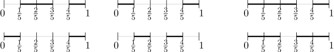
Figure 1: Reduction idea for Theorem 4. Here $n=5$. In both (a) and (b), Alice’s input ${\bf x}$ is shown in the left figure and Bobs input ${\bf y}$ is shown in the middle one. In (a), ${\bf x}=01101$ and ${\bf y}=10001$; $\textsc{Disj}({\bf x},{\bf y})=0$; $l_{A}=\frac{3}{5}$ and $l_{B}=\frac{3}{5}$; the total Klee’s measure is shown in the right figure and the value is $\frac{4}{5}<l_{A}+l_{B}$. In (b), ${\bf x}=10001$ and ${\bf y}=01010$; $\textsc{Disj}({\bf x},{\bf y})=1$; $l_{A}=\frac{2}{5}$ and $l_{B}=\frac{2}{5}$; The total Klee’s measure is shown in the right figure and the value is $\frac{4}{5}=l_{A}+l_{B}$.

Theorem 4.

For every $\epsilon\in(0,0.1)$, there exists an positive integer $n$ such that any randomized one-pass streaming algorithm that outputs $(\epsilon,\rho)$-additive solution to Klee’s measure for all streams of at most $2n$ intervals in $\mathbb{R}$, uses $\Omega\left(\frac{1}{\epsilon}+\log n\right)$ bits of space.

Proof.

We prove the Theorem by proving the followings.

(a)

For every $\epsilon\in(0,0.1)$, there exists an positive integer $n$ such that any randomized one-pass streaming algorithm that outputs $(\epsilon,\rho)$-additive solution to Klee’s measure for all streams of at most $2n$ intervals in $\mathbb{R}$, uses $\Omega\left(\frac{1}{\epsilon}\right)$ bits of space.

(b)

For every $\epsilon\in(0,0.1)$, there exists an positive integer $n$ such that any randomized one-pass streaming algorithm that outputs $(\epsilon,\rho)$-additive solution to Klee’s measure for all streams of at most $2n$ intervals in $\mathbb{R}$, uses $\Omega\left(\log n\right)$ bits of space.

(a) Let $n={\lfloor{\frac{1}{2\epsilon}}\rfloor}-1$ and ${\cal A}$ be a streaming algorithm that returns $(\epsilon,\rho)$-additive solution to Klee’s measure and uses space $s=o\left(\frac{1}{\epsilon}\right)$. The following one-way communication protocol can solve the Disj using space $o(n)$. Alice will process her input ${\bf x}$ as follows. See Figure LABEL:klee_lb. For each $i$, if $x_{i}=1$ then we give the interval $[\frac{i-1}{n},\frac{i}{n}]$ as input to $\mathcal{A}$, otherwise, we do nothing. Let the corresponding set of intervals generated by Alice be $S_{A}$ and $l_{A}$ be the Klee’s measure of $S_{A}$. Alice will send the current memory state of $\mathcal{A}$ and $l_{A}$ to Bob. Similarly, Bob will process his input $\bf y$. Let the corresponding set of intervals generated by Bob be $S_{B}$ and $l_{B}$ be its Klee’s measure. Observe that $\textsc{Disj}({\bf x,y})=1$ if the length of $S_{A}\cup S_{B}$ is $l_{A}+l_{B}$ and in this case $\mathcal{A}$ returns at least $l_{A}+l_{B}-\epsilon$. $\textsc{Disj}({\bf x,y})=0$ if the length of $S_{A}\cup S_{B}$ is at most $l_{A}+l_{B}-\frac{1}{n}<l_{A}+l_{B}-2\epsilon$ and $\mathcal{A}$ returns less then $l_{A}+l_{B}-\epsilon$. So, we report $\textsc{Disj}({\bf x,y})=1$ if and only if $\mathcal{A}$ gives output at least $l_{A}+l_{B}-\epsilon$.

(b) Let $\mathcal{V}$ be a family of $\{0,1\}^{n}$ vectors such that $\forall{\bf x}\in\mathcal{V}$, $\sum\limits_{i=1}^{n}x_{i}=\frac{n}{2}$; $\forall{\bf x},{\bf y}\in\mathcal{V}$ and ${\bf x}\neq{\bf y}$ , there are at most $\frac{n}{4}$ indices where both ${\bf x}$ and ${\bf y}$ have $1$. Such a family $\mathcal{V}$ with $\left|\mathcal{V}\right|=2^{\Omega(n)}$ exists [4]. We define the Equality function as follows. Both Alice and Bob get vectors ${\bf x}$ and ${\bf y}$ respectively from $\mathcal{V}$ and the objective is to decide whether ${\bf x}={\bf y}$. Formally, $\textsc{Equality}({\bf x},{\bf y})=1$ if and only if ${\bf x}={\bf y}$. It is well known that the two-way private coin randomized communication complexity of Equality is $\Omega(\log n)$ [4, 42, 35].

Let $n>2^{1/\epsilon}$ and ${\cal A}$ be a streaming algorithm that returns $(\epsilon,\rho)$-additive solution to Klee’s measure using space $o(\log n)$ bits. The following one-way communication protocol can solve the Equality using space $o(\log n)$. Both Alice and Bob process their input exactly as in part (a). Let $S_{A}$, $S_{B}$, $l_{A}$, $l_{B}$ have the same notation as in (a). Observe that if $\textsc{Equality}({\bf x},{\bf y})=1$, then the length of $S_{A}\cup S_{B}$ is $0.5$ and in this case $\mathcal{A}$ returns at most $0.5+0.1=0.6$. If $\textsc{Equality}({\bf x},{\bf y})=0$, then the length of $S_{A}\cup S_{B}$ is at least $0.75$ and in this case $\mathcal{A}$ returns at least $0.75-0.1=0.65$. Therefore $\textsc{Equality}({\bf x,y})=1$ if and only if $\mathcal{A}$ gives output at most $0.6$. ∎

Remark 1.

• Multipass lower bound: We can also do both of the above reductions from Disj and Equality to a $p$-pass streaming algorithm, using space $s$, for Klee’s measure in $\mathbb{R}$. Observe that the induced protocol for Disj requires at most $2ps$ bits of communication. This implies $s=\Omega\left(\frac{1}{p}\left(\frac{1}{\epsilon}+\log n\right)\right)$.

2.3 Algorithms for Klee’s measure in $[0,1]^{d}$

Randomized algorithm

Let us consider a stream $\mathcal{R}$, where each $R_{i}\subset[0,1]^{d}$. Our objective is to output $\hat{V}$ such that $\left|V-\hat{V}\right|\leq\epsilon$ with probability at least $1-\rho$, where $0<\epsilon,\rho<1$. We generate and store $M$ random points $p_{1},\ldots,p_{M}\in[0,1]^{d}$. For each point $p_{j},j\in[M]$, we maintain a binary indicator random variable $X_{j}$, $j\in[M]$. $X_{j}=1$ if and only if $p_{j}$ lies on or inside any $R_{i}\in\mathcal{R}$. At the end of the stream, we report $\hat{V}=\frac{X}{M}$, where $X=\sum_{i=1}^{M}X_{i}$.

As we have chosen $M$ points uniformly at random, the probability that a random point is present in some rectangle in the stream, is same as the volume of $\bigcup\limits_{i=1}^{n}R_{i}$. So, $\mbox{Pr}(X_{j}=1)=V$ and $\mathbb{E}({X})=MV$. Now apply standard Chernoff bound.

$$\mbox{Pr}\left(\left|V-\hat{V}\right|\geq\epsilon\right) = \mbox{Pr}(\left|X-MV\right|\geq M\epsilon)$$

$$\leq 2e^{-\frac{(\epsilon/V)^{2}}{2+\epsilon/V}MV}$$

$$= 2e^{-\frac{\epsilon^{2}}{2V+\epsilon}M}$$

$$\leq 2e^{-\frac{\epsilon^{2}}{2+\epsilon}M}\leq\rho.$$

This implies $M\geq\frac{2+\epsilon}{\epsilon^{2}}\log\left(\frac{1}{\rho}\right)$. Hence, we have the following theorem.

Theorem 5.

There exists a randomized one-pass streaming algorithm that outputs $(\epsilon,\rho)$-additive solution to Klee’s measure in $[0,1]^{d}$ and uses $O\left(\frac{1}{\epsilon^{2}}\log\left(\frac{1}{\rho}\right)\right)$ space.

Deterministic algorithm

A hyperrectangle $R\subset[0,1]^{d}$ is $\delta$-fat if the length of each side is at least $\delta\in(0,1)$. Our objective is to report a $\hat{V}$ such that $V-\epsilon\leq\hat{V}\leq V$ for a given $\epsilon\in(0,1)$. The main result is stated in the following theorem.

Input: A stream of hyperrectangles $\mathcal{R}=\{R_{1},\ldots,R_{n}\}$ in $[0,1]^{d}$.

Output: Klee’s measure of the stream

1 begin

2       Subdivide $[0,1]^{d}$ into $1/\delta^{d}$ hyperboxes, each of size $\delta\times\ldots\times\delta$ as shown in Figure 2; denote each such hyperbox as $\mathcal{H}^{\delta}_{d}$.

3       We magnify each dimension of $[0,1]^{d}$ by $1/\delta$ so that each $\mathcal{H}^{\delta}_{d}$ becomes $[0,1]^{d}$.

4       Let $\mathcal{B}$ be the set of all magnified ${\mathcal{H}}^{\delta}_{d}$’s.

5      

6      Call in parallel, $1/\delta^{d}$ copies of $ALG(d,\epsilon)$ — one for each $\mathcal{H}_{\delta}^{d}\in\mathcal{B}$. ($ALG(d,\epsilon)$ is given as Algorithm 2.)

7       for (each hyperrectangle $R$ in the stream)  do

8             Find all ${\mathcal{H}_{\delta}^{d}}\in\mathcal{B}$ that intersects $R$ and give $R\cap{\mathcal{H}}_{\delta}^{d}$ as input to the corresponding $ALG(d,\epsilon)$ algorithm for ${\mathcal{H}}^{\delta}_{d}$.

9       end for

10      

11      Find the sum of outputs produced by all $1/\delta^{d}$ copies of $ALG(d,\epsilon)$ and multiply by $\delta^{d}$ and return.

12 end

13

Algorithm 1 Klee($d,\epsilon$)

Theorem 6.

There exists a deterministic one-pass streaming algorithm that takes a stream of $\delta$-fat hyperrectangles in $[0,1]^{d}$ as input, and outputs $\hat{V}$ such that $V-\epsilon\leq\hat{V}\leq V$, using $O\left(\frac{2^{d^{2}+d}}{\epsilon^{d-1}\delta^{d}}\right)$ space, where $\epsilon\in(0,1)$ is an input parameter.

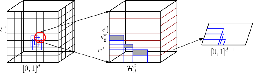
Figure 2: The figure to the left shows the placement of some input rectangles in $[0,1]^{d}$, the figure in the middle shows anchored rectangle at origin in $[0,1]^{d}$ and the figure to the right shows projection of all intersection of all rectangles with a particular strip to $[0,1]^{d-1}$.

Proof.

The crux of the proof is to subdivide $[0,1]^{d}$ into $1/\delta^{d}$ hyperboxes, each of size $\delta\times\ldots\times\delta$ as shown in Figure 2; denote each such hyperbox as $\mathcal{H}^{\delta}_{d}$. Each $\delta$-fat hyperrectangle of the stream will intersect at least one corner of some $\mathcal{H}^{\delta}_{d}$; there are $2^{d}$ such corners for each ${\mathcal{H}}^{\delta}_{d}$. For any corner, a subset of hyperrectangles of $\mathcal{R}$ will be called anchored if each member of the subset intersects that corner point. A set of hyperrectangles is anchored for a hyperbox if each hyperrectangle in the set intersects at least one corner of the hyperbox. The next Claim, proved later, finds the estimate of klee’s measure for hyperrectangles that are anchored for a hyperbox.

Claim 7.

Let ${\mathcal{R}}_{a}$ be a stream of hyperrectangles anchored for $[0,1]^{d}$. There exists a deterministic one-pass streaming algorithm that outputs $\hat{V_{a}}$ such that $V_{a}-\epsilon\leq\hat{V_{a}}\leq V_{a}$ and uses $O\left(\frac{2^{d^{2}+d}}{\epsilon^{d-1}}\right)$ space, where $V_{a}$ is the Klee’s measure of ${\mathcal{R}}_{a}$ and $\epsilon\in(0,1)$ is an input parameter.

To put the proof of Theorem 6 in Claim 7’s context of $[0,1]^{d}$, we magnify each dimension of $[0,1]^{d}$ by $1/\delta$ so that each $\mathcal{H}^{\delta}_{d}$ becomes $[0,1]^{d}$. The error term will also change accordingly. So, our problem boils down to finding the Klee’s measure in $[0,1/\delta]^{d}$ within an additive error of $\epsilon/\delta^{d}$. Let $\mathcal{B}$ be the set of all magnified ${\mathcal{H}}^{\delta}_{d}$. Recall that each hyperrectangle $R\in\mathcal{R}$ is $\delta$-fat. Therefore, for each ${\mathcal{H}}^{\delta}_{d}\in\mathcal{B}$, if $R\cap{\mathcal{H}}^{\delta}_{d}\neq\phi$, then $R\cap\mathcal{H}_{\delta}^{d}$ is anchored at (at least) one of the corners of ${\mathcal{H}}^{\delta}_{d}$.

We start, in parallel, $1/\delta^{d}$ $d$-dimensional anchored Klee’s measure algorithm – one for each $\mathcal{H}_{\delta}^{d}\in\mathcal{B}$. On receiving a rectangle $R$, we find all ${\mathcal{H}_{\delta}^{d}}\in\mathcal{B}$ that intersects $R$ and give $R\cap{\mathcal{H}}_{\delta}^{d}$ as input to the corresponding algorithm for ${\mathcal{H}}^{\delta}_{d}$. Refer the pseudocode given in Algorithm 1. Total additive error of $\epsilon/\delta^{d}$ can be achieved if we can ensure additive error of at most $\epsilon$ for each ${\mathcal{H}}^{\delta}_{d}\in\mathcal{B}$. By Claim 7, this can be achieved by using $O\left(\frac{2^{d^{2}+d}}{\epsilon^{d-1}}\right)$ space for each ${\mathcal{H}}^{\delta}_{d}$. Hence, the total amount space required is $O\left(\frac{2^{d^{2}+d}}{\epsilon^{d-1}\delta^{d}}\right)$. ∎

Proof of Claim 7.

We will prove it by using induction on $d$, where $d\geq 1$. Let $ALG(\epsilon,d)$ be the algorithm that solves the problem within an additive error of $E(\epsilon,d)$ using $S(\epsilon,d)$ space. We have to prove that $E(\epsilon,d)\leq\epsilon$ and $S(\epsilon,d)\leq\frac{2^{d^{2}+d}}{\epsilon^{d-1}},~{}\mbox{where}~{}d\geq 1$. For the base case of $d=1$, each interval of the stream in $[0,1]$ is anchored either at 0 or 1. Our algorithm $ALG(\epsilon,1)$ maintains the rightmost (leftmost) extreme point left (right) of all intervals anchored at 0 (1). At the end of the stream, we report $\min(\mbox{{\em left}}+\mbox{{\em right}},1)$. Observe that we output exact Klee’s measure without any error using constant space. Hence, $E(\epsilon,1)=0\leq\epsilon~{}\mbox{and}~{}S(\epsilon,1)=O(1)$.

Assuming the statement is true for all dimensions less than or equal to $d-1$, we show that it is also true for dimension $d$. We divide the entire space $[0,1]^{d}$ along the $d$-th dimension into $1/\epsilon^{\prime}$ strips, each of the form $[0,1]^{d-1}\times[(i-1)\epsilon^{\prime},i\epsilon^{\prime}]$, where $\epsilon^{\prime}=\epsilon/2^{d+1}$ and $1\leq i\leq 1/\epsilon^{\prime}$. We start $1/\epsilon^{\prime}$ copies of the algorithm $ALG(\epsilon/2,d-1)$, one for each strip.

On receiving an anchored hyperrectangle $R\subset[0,1]^{d}$, we assign it to one of the $2^{d}$ corners with which it intersects. Without loss of generality, assume that it is anchored at the origin. Let $R$ cut through $p$ strips $(0\leq p\leq 1/\epsilon^{\prime})$ and extend for a distance of $q$ $(0\leq q<\epsilon^{\prime})$ in the last strip along the $d$-th dimension. Refer Figure 2. Thus $R$ can be decomposed as $R=R^{\prime}\times[0,p\epsilon^{\prime}+q]$, where $R^{\prime}\mbox{ (of dimension $d-1$) }\subset[0,1]^{d-1}$. Divide $R$ into $p$ parts of the form $R^{\prime}\times[(j-1)\epsilon^{\prime},j\epsilon^{\prime}]$, where $j\in[p]$ and assign $R^{\prime}\times[(j-1)\epsilon^{\prime},j\epsilon^{\prime}]$ to the $j$-th strip. Part of hyperrectangles we are assigning to a strip is of length $\epsilon^{\prime}$ along dimension $d$. So, each anchored hyperrectangle in $[0,1]^{d}$ assigned to a strip can be thought of as a $d-1$ dimensional hyperrectangle with a length of $\epsilon^{\prime}$ along the $d$-th dimension. Observe that the projection of hyperrectangles of the form $R^{\prime}\times[(j-1)\epsilon^{\prime},j\epsilon^{\prime}]$, that belong to a particular strip $j$, to the $d-1$ dimensional space is nothing but $R^{\prime}$. See Figure 2 for an example. For each $j\in[p]$, $R^{\prime}$ is given as an input to the coresponding $ALG(\epsilon/2,d-1)$ of the $j^{th}$ strip. At the end of the stream, we compute the sum of outputs produced by all $\frac{1}{\epsilon^{\prime}}$ recursive calls $ALG(\epsilon/2,d-1)$ and then multiply by $\epsilon^{\prime}$ to get the final estimate of Klee’s measure. Refer the pseudocode given in Algorithm 2.

Input: A stream of hyperrectangles in $[0,1]^{d}$ anchored either at $0$ or $1$.

Output: Klee’s measure of the stream

1 begin

2       Divide the entire space $[0,1]^{d}$ along the $d$-th dimension into $1/\epsilon^{\prime}$ strips, where $\epsilon^{\prime}=\epsilon/2^{d+1}$, such that each strip is of the form $[0,1]^{d-1}\times[(i-1)\epsilon^{\prime},i\epsilon^{\prime}]$, $1\leq i\leq 1/\epsilon^{\prime}$.

3       We start $1/\epsilon^{\prime}$ copies of the algorithm $\mbox{ALG}(d-1,\epsilon/2)$, one for each strip.

4       for (each anchored hyperrectangle $R$ in the stream)  do

5             Assign $R$ to one of the $2^{d}$ corners with which it intersects. W.l.o.g., assume that it is anchored at the origin.

6             Let $R=R^{\prime}\times[0,p\epsilon^{\prime}+q]$, where $R^{\prime}\subset[0,1]^{d-1}$, $0\leq p\leq 1/\epsilon^{\prime}$ and $0\leq q<\epsilon^{\prime}$. Divide $R$ into $p$ parts of the form $R^{\prime}\times[(j-1)\epsilon^{\prime},j\epsilon^{\prime}]$, where $j\in[p]$ and assign $R^{\prime}\times[(j-1)\epsilon^{\prime},j\epsilon^{\prime}]$ to the $j$-th strip. Ignore remaining portion of $R$, i.e, $R^{\prime}\times[p\epsilon^{\prime},p\epsilon^{\prime}+q]$ (the shaded part in Figure 2).

7             For each $j\in[p]$, give input $R^{\prime}$ to the corresponding $\mbox{ALG}(d-1,\epsilon/2)$ of the $j$-th strip.

8            

9       end for

10      Find the sum of outputs produced by all $1/\epsilon^{\prime}$ recursive calls $\mbox{ALG}(d-1,\epsilon/2)$ and then multiply by $\epsilon^{\prime}$ and return.

11 end

12

Algorithm 2 ALG($d,\epsilon$): $d$ dimensional anchored Klee’s measure, $d>1$

Our algorithm incurs two types of errors –

(i)

Error incurred from the recursive calls to the lower dimensions.

(ii)

The error incurred at this level of the recursion corresponding to the top part of $R$, i.e., $R^{\prime}\times[p\epsilon^{\prime},p\epsilon^{\prime}+q]$ (as shown by the shaded parts in Figure 2) that we just ignore.

To analyze the error of type (ii), notice that these top parts of the hyperrectangles anchored at a corner has a special structure as these hyperrectangles form a partial order under inclusion. So, the errors are additive and can be at most $\epsilon^{\prime}$. Hence, the total error with respect to all $2^{d}$ corners is at most $2^{d}\epsilon^{\prime}$. Now to estimate the error of type (i), we observe that the error in calculation of Klee’s measure due to one strip (because of the multiplication by $\epsilon^{\prime}$) is $\epsilon^{\prime}E(\epsilon/2,d-1)$. So, the total error with respect to all the $1/\epsilon^{\prime}$ strips is $\frac{1}{\epsilon^{\prime}}(\epsilon^{\prime}E(\epsilon,d-1))=E(\epsilon,d-1)$ which by induction hypothesis is at most $\epsilon/2$. Now considering the fact that $\epsilon^{\prime}=\epsilon/2^{d+1}$, the total error is given by

$$E(\epsilon,d)=2^{d}\epsilon^{\prime}+E(\epsilon/2,d-1)\leq\epsilon$$

.

With the space requirement for one strip being $S(\epsilon/2,d-1)$ by induction hypothesis, the total space requirement with respect to all $1/\epsilon^{\prime}$ strips is $\frac{1}{\epsilon^{\prime}}S(\epsilon/2,d-1)$ along with the book keeping of $\frac{1}{\epsilon^{\prime}}$ instances of $ALG(\epsilon/2,d-1)$. Therefore,

$$S(\epsilon,d)\leq\frac{1}{\epsilon^{\prime}}S(\epsilon/2,d-1)+\log\left(\frac{1}{\epsilon^{\prime}}\right)=\frac{2^{d+1}}{\epsilon}S(\epsilon/2,d-1)+\log\left(\frac{2^{d+1}}{\epsilon^{\prime}}\right)\leq\frac{2^{d^{2}+d}}{\epsilon^{d-1}}.$$

∎

3 CONVEX-BODY and GEOM-QUERY-CONV-POLY

In this section, we first strengthen the lower bound result on convex hull by showing that even promised version in hand. Next, we derive lower bounds for convex body approximation and point existence queries in a convex polygon followed by algorithms for them. To the best of our knowledge, the lower bound on convex body approximation is first of this kind. As a consequence of our result on convex body approximation, we can solve LP in the streaming model and design a property testing type result for geometric queries.

3.1 Lower bounds

Lower bound for promise version of convex hull

Theorem 8.

Any randomized one-pass streaming algorithm for convex hull that distinguishes between inputs having $\left|\mathcal{CH}(\mathcal{P})\right|=O(1)$ and $\left|\mathcal{CH}(\mathcal{P})\right|=\Omega(n)$ in $\mathbb{R}^{2}$ with probability $1-\rho$, uses $\Omega(n)$ bits of space.

Proof.

If there exists a randomized algorithm $\mathcal{A}$ that distinguishes between $\left|\mathcal{CH}(\mathcal{P})\right|=O(1)$ and $\left|\mathcal{CH}(\mathcal{P})\right|=\Omega(n)$ with probability $\rho$ and uses $o(n)$ bits, we can show the existence of a randomized protocol that solves Index and uses $o(n)$ bits. Consider a regular convex polygon of $2n$ vertices, $V=\{v_{i}:1\leq i\leq 2n\}$, as shown in Figure 3. We construct the input point set $\mathcal{P}$ to $\mathcal{A}$ by taking each $v_{2i-1},1\leq i\leq n$. We also add $v_{2i}$ if and only if the $i$-th bit of Alice’s input $x_{i}=1$. We send the current sketch to Bob. Let $j$ be Bob’s query index. Now another $n+2$ points are given as input to $\mathcal{A}$ such that $n$ of them are in convex position inside the triangle $\Delta v_{2j-1}v_{2j}v_{2j+1}$ and the other two are such that no vertices of $V\setminus\{v_{2j-1},v_{2j},v_{2j+1}\}$ can be on $\mathcal{CH}(\mathcal{P})$ as shown in Figure 3. Observe that the last $n+2$ points are put in such a way that if $v_{2j}$ is on $\mathcal{CH}(\mathcal{P})$ then $\left|\mathcal{CH}(\mathcal{P})\right|=5$, otherwise, $\left|\mathcal{CH}(\mathcal{P})\right|=n+4=\Omega(n)$. Note that by construction $v_{2j}$ is on $\mathcal{CH}(\mathcal{P})$ if and only if $x_{j}=1$. Hence, $x_{j}=1$ if $\left|\mathcal{CH}(\mathcal{P})\right|=5$ and $x_{j}=0$ if $\left|\mathcal{CH}(\mathcal{P})\right|=\Omega(n)$. ∎

Figure 3: $u$, $v$ and the dotted points inside the triangle $\Delta v_{2j-1}v_{2j}v_{2j+1}$ are the last $n+2$ points.

Lower bound for convex body approximation and geometric query

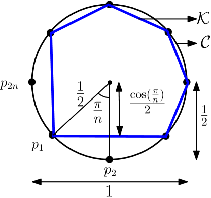
Figure 4: Reduction idea for Theorem 9.

Theorem 9.

For every $\epsilon>0$, there exists a positive integer $n$ such that any (one-pass streaming) algorithm that $(\epsilon,\rho)$-approximates a convex polygon $\mathcal{K}$, requires $\Omega\left(\frac{1}{\sqrt{\epsilon}}\right)$ bits of space, where $\mathcal{K}$ is given as a stream of at most $2n$ straight lines in $\mathbb{R}^{2}$.

Proof.

Without loss of generality, assume that $0<\epsilon<\frac{1}{2}$. Let $n={\lceil{\frac{\pi}{2\sqrt{2\epsilon}}}\rceil}$ and $\mathcal{A}$ be a (streaming) algorithm, as stated, using $o\left(\frac{1}{\sqrt{\epsilon}}\right)$ bits. Now we can design a protocol that solves Index using space $o(n)$. See Figure 4 for the following discussion.Alice and Bob know a circle $\mathcal{C}$ of diameter 1 and $2n$ points $p_{1},\ldots,p_{2n}$ placed evenly on its circumference. We process Alice’s input ${\bf x}$ as follows. If $x_{i}=1$, then we give two line segments $\overline{p_{2i-1}p_{2i}}$ and $\overline{p_{2i}p_{2i+1}}$ as inputs to $\mathcal{A}$. If $x_{i}=0$, we give the line segment $\overline{p_{2i-1}p_{2i+1}}$ as an input to $\mathcal{A}$. We send the current memory state of Alice to Bob. Let $\mathcal{K}$ be the actual convex polygon and $\mathcal{K}^{\prime}$ be the convex polygon generated by $\mathcal{A}$ such that $d_{H}(\mathcal{K},\mathcal{K}^{\prime})\leq\epsilon$. Observe that $x_{i}=1$ implies $p_{2i}\in\mathcal{K}$, i.e., there exists a point $q\in\mathcal{K}^{\prime}$ such that $d(p_{2i},q)\leq\epsilon$, where $d(p,q)$ is the Euclidean distance between $p$ and $q$. If $x_{i}=0$, then $p_{2i}\notin\mathcal{K}$ and $d(p_{2i},\mathcal{K})=\min\limits_{q\in\mathcal{K}}d(p,q)=\frac{1-\cos\left(\frac{\pi}{n}\right)}{2}=\sin^{2}\left(\frac{\pi}{2n}\right)\geq\sin^{2}\sqrt{2\epsilon}>\epsilon$, as $0<\epsilon<\frac{1}{2}$.

Let $j$ be the query index of Bob. We report $x_{j}=1$ if and only if $\mathcal{C}(p_{2j})\cap\mathcal{K}^{\prime}\neq\phi$, where $\mathcal{C}(p)$ denotes the circle of radius $\epsilon$ centred at $p$. ∎

The proof for the lower bound of geom-query-conv-poly is similar to the proof of Theorem 9.

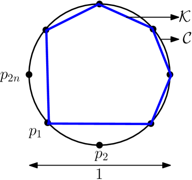
Figure 5: Reduction idea for Theorem 10.

Theorem 10.

Every randomized one-pass streaming algorithm that solves geom-query-conv-poly with probability $1-\rho$, uses $\Omega(n)$ bits of space.

Proof.

Let $\mathcal{A}$ be a streaming algorithm, as stated in the Theorem, using $o(n)$ bits. Now we can design a protocol that solves Index using space $o(n)$ bits. See Figure 5 for the following discussion. Alice and Bob know a circle $\mathcal{C}$ of diameter 1 and $2n$ points $p_{1},\ldots,p_{2n}$ placed evenly on its circumference. We process Alice’s input ${\bf x}$ as follows. If $x_{i}=1$, then we give two line segments $\overline{p_{2i-1}p_{2i}}$ and $\overline{p_{2i}p_{2i+1}}$ as inputs to $\mathcal{A}$. If $x_{i}=0$, we give the line segment $\overline{p_{2i-1}p_{2i+1}}$ as an input to $\mathcal{A}$. We send the current memory state of Alice to Bob.

Let $\mathcal{K}$ be the actual convex polygon. Observe that $x_{i}=1$ implies $p_{2i}\in\mathcal{K}$. If $x_{i}=0$, then $p_{2i}\notin\mathcal{K}$. Let $j$ be the query index of Bob. We report $x_{j}=1$ if and only if $\mathcal{A}$ reports $p_{2j}\in\mathcal{K}$. ∎

3.2 Algorithms

Convex body approximation

We state Dudley’s result [19] and some observations about Hausdroff distance that will be useful for the algorithm.

Lemma 11.

[19] A convex body $\mathcal{K}$ can be $\epsilon$-approximated by a polytope $P$ with $1/{\epsilon^{(d-1)/2}}$ facets. $\epsilon$-approximation in this context means $d_{H}(\mathcal{K},P)\leq\epsilon$.

Observation 12.

Let $\mathcal{K}_{1},\mathcal{K}_{2},\mathcal{K}_{1}^{\prime}$ and $\mathcal{K}_{2}^{\prime}$ be convex bodies with $\mathcal{K}_{1}\subseteq\mathcal{K}_{1}^{\prime}$, $\mathcal{K}_{2}\subseteq\mathcal{K}_{2}^{\prime}$ and $d_{H}(\mathcal{K}_{1},\mathcal{K}_{1}^{\prime})\leq\epsilon_{1},d_{H}(\mathcal{K}_{2},\mathcal{K}_{2}^{\prime})\leq\epsilon_{2}$. Then $d_{H}(\mathcal{K}_{1}\cap\mathcal{K}_{2},\mathcal{K}_{1}^{\prime}\cap\mathcal{K}_{2}^{\prime})\leq\max(\epsilon_{1},\epsilon_{2})$.

Observation 13.

Let $\mathcal{K},~{}\mathcal{K}^{\prime}$ and $~{}\mathcal{K}^{\prime\prime}$ be convex bodies such that $d_{H}(\mathcal{K},\mathcal{K}^{\prime})\leq\epsilon_{1}$ and $d_{H}(\mathcal{K}^{\prime},\mathcal{K}^{\prime\prime})\leq\epsilon_{2}$. Then, $d_{H}(\mathcal{K},\mathcal{K}^{\prime\prime})\leq\epsilon_{1}+\epsilon_{2}$.

Note that the approximated convex body in Lemma 11 is always a superset of the original one. Given a convex body $\mathcal{K}$ in $\mathbb{R}^{d}$ and a parameter $\epsilon>0$, let $\mathcal{A}$ be a non-streaming algorithm that outputs a convex polytope $\mathcal{K}^{\prime}$ such that $d_{H}(\mathcal{K},\mathcal{K}^{\prime})\leq\epsilon$ and $\mathcal{A}$ stores $\frac{1}{\epsilon^{(d-1)/2}}$ facets. Agarwal et al. [2] used Bentley-Saxe’s dynamization technique [10] to maintain the approximate extent measures of a point set. We adapt these ideas for hyperplanes. Let a convex body $\mathcal{K}$ be given as a stream of hyperplanes in $\mathbb{R}^{d}$. $\mathcal{K}$ is contained in a unit ball $\mathcal{B}$. Note that $\mathcal{K}$ is the intersection of all hyperplanes in the stream. The objective is to store a convex body $\mathcal{K}^{\prime}$ using sub-linear number of facets that will $\epsilon$-approximate $\mathcal{K}$, i.e., $d_{H}(\mathcal{K},\mathcal{K}^{\prime})\leq\epsilon$.

We partition the processed stream of hyperplanes $\mathcal{H}=<H_{1},\ldots,H_{n}>$ into $t$ parts — $\mathcal{H}_{1},\ldots,\mathcal{H}_{t}$, $t\leq{\lceil{\log n}\rceil}$. For each $i\in[t]$, $\left|\mathcal{H}_{i}\right|=2^{r_{i}}$ for some non-negative integer $r_{i}<{\lceil{\log n}\rceil}$. We say $r_{i}$ is the rank of $\mathcal{H}_{i}$. We maintain our data structure in a such a way that the rank of $\mathcal{H}_{i}$ is equal to the rank of $\mathcal{H}_{j}$ if and only if $i=j$. Let $C_{i}=\bigcap\limits_{H\in\mathcal{H}_{i}}H$, be the convex polytope of hyperplanes in $\mathcal{H}_{i}$. As we can not store $\mathcal{H}_{i}$ or $C_{i}$, we maintain some approximation $C_{i}^{\prime}$ of $C_{i}$ such that $d_{H}(C_{i},C_{i}^{\prime})\leq f(r_{i})$. $f(r)=\epsilon/2r^{2}$ if $r\neq 0$ and $f(0)=0$. We store $C^{\prime}_{i}$ and $r_{i}$. Let $\mathcal{C}=\{C^{\prime}_{1},\ldots,C^{\prime}_{t}\}$.

Now consider the situation when we have to process $H_{n+1}$. We set $\mathcal{H}_{0}=\{H_{n+1}\}$ and add $C^{\prime}_{0}=C_{0}=H_{n+1}\cap\mathcal{B}$ to $\mathcal{C}$ as $f(0)$ approximation of $C_{0}$. If there exists $C^{\prime}_{i},C^{\prime}_{j}\in\mathcal{C}$ such that $r_{i}$ $=$ $r_{j}$ $=$ $r$ for some $r<{\lceil{\log(n+1)}\rceil}$, then using algorithm $\mathcal{A}$, we find $C^{\prime}$ as approximation of $C^{\prime}_{i}\cap C^{\prime}_{j}$ such that $d_{H}(C^{\prime},C^{\prime}_{i}\cap C^{\prime}_{j})\leq f(r+1)$. Note that the actual convex body corresponding to $C^{\prime}$ i.e., $\mathcal{H}_{i}\cap\mathcal{H}_{j}$ is of rank $r+1$. $\mathcal{C}=(\mathcal{C}\setminus\{C_{i},C_{j}\})\cup\{C^{\prime}\}$. We repeat the same process until all members of $\mathcal{C}$ have distinct rank. Now our target is that at the end, we should have each $C_{i}^{\prime}$ as approximation of $C_{i}$ such that $d_{H}(C_{i},C^{\prime}_{i})\leq\epsilon$. As a result, we get $\mathcal{K}^{\prime}=\bigcap\limits_{i=1}^{t}C^{\prime}_{i}$ as an approximation of $\mathcal{K}=\bigcap\limits_{i=1}^{t}C_{i}$ such that $d_{H}(\mathcal{K},\mathcal{K}^{\prime})\leq\epsilon$ by Observation 12. Note that the number of times a $C_{i}$ is approximated is at most its rank. Hence by Observation 13, we have

$$d_{H}(C_{i},C^{\prime}_{i})\leq\sum\limits_{l=1}^{r}f(l)=\sum\limits_{l=1}^{r}\frac{\epsilon}{2l^{2}}\leq\epsilon.$$

By Lemma 11, the amount of space used to store $C^{\prime}_{i}$ is $O\left(\frac{1}{f(r)^{(d-1)/2}}\right)$ where $r$ is the rank of $\mathcal{H}_{i}$. We consider only for $r>0$, because there can be at most one $C_{i}$ of rank $0$ and the corresponding approximation stores only $1$ facet. Hence, the total amount of space we use is

$$1+\sum_{l=1}^{t}\left|C^{\prime}_{i}\right|=O\left(\sum\limits_{l=1}^{{\lceil{\log n}\rceil}}\frac{1}{(f(l))^{(d-1)/2}}\right)=O\left(\sum\limits_{l=1}^{{\lceil{\log n}\rceil}}\frac{1}{(\epsilon/2l)^{(d-1)/2}}\right)=O\left(\frac{\log^{d}n}{\epsilon^{(d-1)/2}}\right)$$

.

We summarize the above discussion in the following Theorem.

Theorem 14.

A convex body $\mathcal{K}$, given as stream of $n$ hyperplanes, can be $\epsilon$-approximated deterministically by a polytope $P$ with $O\left(\frac{\log^{d}n}{\epsilon^{(d-1)/2}}\right)$ facets.

Low dimensional LP

Chan et al. [11] gave a multi-pass algorithm to find exact solution to LP, whose one-pass counterpart admits a lower bound of $\Omega(n)$ bits of space [24].

In the streaming setting of LP, constraints arrive as a stream of hyperplanes. Note that in LP, the feasible region, i.e., intersection of all constraints (hyperplanes) is a convex body. Due to Theorem 14, given a set of contraints as a stream, we can maintain $\epsilon$-approximation of the convex body, i.e., the feasible region of the LP using polylogarithmic  space. The $\epsilon$-approximation along with the objective function can be used to find an $\epsilon$-additive solution to LP. Note that the $\epsilon$-approximtaion of the convex body is a superset of original convex body. So, the extreme point of the approximated convex body in the direction of the objective function vector may lie outside the feasible region. One can shift the facets of the approximated convex body $\epsilon$ distance inwards to get a feasible solution also. An added advantage is that the objective function need not be known beforehand. In summary, we have the following Corollary to Theorem 14.

Corollary 15.

There exists a one-pass deterministic streaming algorithm that outputs $\epsilon$-additive solution to LP using $O\left(\frac{\log^{d}n}{\epsilon^{(d-1)/2}}\right)$ space for a fixed dimension $d$. The objective function may be revealed at the end of the stream of contraints.

Property testing result for GEOM-QUERY-CONV-POLY

By the method discussed in Theorem 14, we approximate $\mathcal{K}$ by a convex body $\mathcal{K}^{\prime}$ such that $\mathcal{K}\subseteq\mathcal{K}^{\prime}$ and $d_{H}(\mathcal{K},\mathcal{K}^{\prime})\leq\epsilon$. By Theorem 14, the amount of space required to maintain $\mathcal{K}^{\prime}$ is $O\left(\frac{\log^{d}n}{\epsilon^{(d-1)/2}}\right)$ facets. Note that at the end of the stream we have $\mathcal{K}^{\prime}$ as our sketch and our objective is to answer correctly for query point $q$ if $d_{H}(\mathcal{K},\mathcal{K}^{\prime})\geq\epsilon$. For geom-query-conv-poly, we report (i) $q\in\mathcal{K}$ if $q\in\mathcal{K}^{\prime}$ and $d_{H}(q,\mathcal{K}^{\prime})\geq\epsilon$, (ii) $q\notin\mathcal{K}$ if $q\notin\mathcal{K}^{\prime}$ and (iii) arbitrary answer, otherwise. See Figure 6. Summarizing the above discussion, we have the following Corollary to Theorem 14.

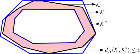
Figure 6: $\mathcal{K}$ is the original convex body. $\mathcal{K}^{\prime}$ is the $\epsilon$-approximation to $\mathcal{K}$. $\mathcal{K}^{\prime\prime}$ is shown as an $\epsilon$ shrink of $\mathcal{K}$. The region inside $\mathcal{K}^{\prime\prime}$ and outside $\mathcal{K}^{\prime}$ are the zones for $q$ where we can correctly answer.

Corollary 16.

There exists a deterministic one-pass streaming algorithm that given a convex polyhedron $\mathcal{K}$ as a stream of hyperplanes and a query point $q$ such that $d_{H}(q,\mathcal{K})\geq\epsilon$, solves geom-query-conv-poly by storing $O\left(\frac{\log^{d}n}{\epsilon^{(d-1)/2}}\right)$ facets.

4 Discrepancy problems

The proofs in this Section will require the notion of star discrepancy [34]. In star discrepancy, all other problem specifications in the definition of discrepancy remain the same but each interval is constrained to have its left end point at $0$.

Thus, the problem of star-geometric-discrepancy is to report

$$D_{g}^{*}(\mathcal{P}):=\sup\limits_{[0,q]\subseteq[0,1]}\left|q-\frac{n_{0q}}{n}\right|,$$

and the problem of star-color-discrepancy is to report

$$D_{c}^{*}(\mathcal{P}):=\stackrel{{\scriptstyle[}}{{I=[0,x]\subseteq[0,1)}}]{\max}{}\left|R(I)-B(I)\right|,$$

which is same as

$$D_{c}^{*}(\mathcal{P})=\stackrel{{\scriptstyle[}}{{I_{p}=[0,p]:p\in\mathcal{P}}}]{\max}{}\left|R(I_{p})-B(I_{p})\right|$$

because discrepancy values at points of the stream $\mathcal{P}$ only matter. The following relations are known between the values of geometric discrepancy $D_{g}(\mathcal{P})$ and color discrepancy $D_{c}(\mathcal{P})$ and their star variants.

Fact 17.

[34] $D_{g}^{*}(\mathcal{P})\leq D_{g}(\mathcal{P})\leq 2D_{g}^{*}(\mathcal{P})$ and $D_{c}^{*}(\mathcal{P})\leq D_{c}(\mathcal{P})\leq 2D_{c}^{*}(\mathcal{P})$.

Fact 18.

[34] Let $x_{1}<x_{2}<x_{3}<\ldots<x_{n}\in[0,1]$ be a sorted sequence of points in $\mathcal{P}$. Then, the supremum in the definition of $D_{g}^{*}$ can be replaced by a maximum operation as $D_{g}^{*}(\mathcal{P})=\max\limits_{i\in[n]}|x_{i}-\frac{2i-1}{2n}|$.

4.1 Problem GEOMETRIC-DISCREPANCY

Theorem 19.

For any $\epsilon>0$, there exists a positive integer $n$ such that any one-pass randomized streaming algorithm that outputs an $(\epsilon,\rho)$-additive solution to geometric-discrepancy for all streams of length $n$, requires $\Omega\left(\frac{1}{\epsilon}\right)$ bits of space.

Proof.

Let $\mathcal{P}$ be the stream. We need the following claim that will be proved later.

Claim 20.

For any $\epsilon>0$, there exists a positive integer $n$ such that any one-pass randomized streaming algorithm that outputs an approximate solution $D$ to star-geometric-discrepancy with probability $\rho$, such that $D_{g}^{*}(\mathcal{P})-\epsilon\leq D\leq 2D_{g}^{*}(\mathcal{P})+\epsilon$, requires $\Omega\left(\frac{1}{\epsilon}\right)$ bits of space, where $\mathcal{P}$ is the input stream of length $2n$.

Let there exist an algorithm as stated in Theorem 19 that returns $D^{\prime}$ for $\epsilon$-additive error solution to geometric-discrepancy and uses space $o\left(\frac{1}{\epsilon}\right)$ bits. Observe that $D_{g}(\mathcal{P})-\epsilon\leq D^{\prime}\leq D_{g}(\mathcal{P})-\epsilon$. Now using Fact 17, we can have the following. $D^{\prime}\leq D_{g}(\mathcal{P})+\epsilon\leq 2D_{g}^{*}(\mathcal{P})+\epsilon$ and $D^{\prime}\geq D_{g}(\mathcal{P})-\epsilon\geq D_{g}^{*}(\mathcal{P})-\epsilon$. So, we can report $D^{\prime}$ as $D$, i.e., the solution to our star-geometric-discrepancy problem satisfying $D_{g}^{*}(\mathcal{P})-\epsilon\leq D\leq 2D_{g}^{*}(\mathcal{P})+\epsilon$. Note that we are using $o\left(\frac{1}{\epsilon}\right)$ bits, which contradicts Claim 20. ∎

Figure 7: Reduction idea for Claim 20. Here $n=3$. In (a), Alice’s input ${\bf x}=010$ and Bob’s input ${\bf y}=100$; $\textsc{Disj}({\bf x},{\bf y})=1$; $D_{g}^{*}(\mathcal{P})=\frac{1}{12}$. In (b), ${\bf x}=011$ and ${\bf y}=110$; $\textsc{Disj}({\bf x},{\bf y})=0$; $D_{g}^{*}(\mathcal{P})=\frac{1}{6}+\frac{1}{24}$.

Proof of Claim 20.

Let $n={\lceil{\frac{1}{32\epsilon}}\rceil}$ and $\mathcal{A}$ be a streaming algorithm that gives output, as stated, using $o\left(\frac{1}{\epsilon}\right)$ bits of space. We design a protocol for solving Disj using $o(n)$ bits. The idea is to generate points at varying intervals as per the inputs of Alice and Bob so that Disj can be solved by looking at the separation of the discrepancy values. We process Alice’s bit vector ${\bf x}$ as follows. See Figure 7, $1_{A}$ ($1_{B}$) denotes an input of $1$ for Alice (Bob) and $0_{A}$ ($0_{B}$) denotes an input of $1$ for Alice (Bob). For each $i\in[n]$, we give $z_{i}$ as input to $\mathcal{A}$ such that $z_{i}=\frac{4i-3}{4n}+\frac{1}{4n}$ if $x_{i}=0$ and $z_{i}=\frac{4i-3}{4n}-\frac{1}{4n}$, otherwise. Let $Z_{A}=\cup_{i=1}^{n}z_{i}$. We send the current memory state to Bob. We process Bob’s input ${\bf y}$ as follows and give another $n$ inputs to $\mathcal{A}$. We give input $z_{n+i}=\frac{4i-1}{4n}$ if $y_{i}=0$ and $z_{n+i}=\frac{4j-3}{4n}-\frac{1}{8n}$ if $y_{i}=1$. Let $Z_{B}=\cup_{i=1}^{n}z_{n+i}$ and $Z=Z_{A}\cup Z_{B}$. In total, we have given $Z$ having $2n$ inputs to $\mathcal{A}$. Let $Z_{s}=<z_{1}^{\prime},\ldots,z_{2n}^{\prime}>$, be the sorted sequence, in increasing fashion, of the points in $Z$. Recalling Fact 18, note that $D_{g}^{*}(\mathcal{P})=\max\limits_{i\in[2n]}D_{i}$, where $D_{i}=\left|\frac{2i-1}{4n}-z_{i}^{\prime}\right|$. Let $J=\{j:y_{j}=1\}$ be the set of indices where Bob has an input of 1. Let $A(j),B(j)$, $j\in J$, be the indices of the input in $Z_{s}$ corresponding to $z_{j}$ (Alice) and $z_{n+j}$ (Bob), respectively. Note that $B(j)=A(j)+1$ if $x_{j}=1$ and $B(j)=A(j)-1$, otherwise . One can see that $D_{i}\leq\frac{1}{4n}$, $\forall i\in[2n]~{}\mbox{and}~{}i\neq A(j),B(j);j\in J$. If $x_{j}=1$, $B(j)=A(j)+1$, $D_{A(j)}=\frac{1}{4n}$ and $D_{B(j)}=\frac{1}{2n}+\frac{1}{8n}$. If $x_{j}=0$, $B(j)=A(j)-1$, $D_{A(j)}=\frac{1}{4n}$ and $D_{B(j)}=\frac{1}{8n}$. Hence, if $\textsc{Disj}({\bf x,y})=0$, there exists an index $i\in[n]$ such that $x_{i}=y_{i}$, then $D_{g}^{*}(\mathcal{P})=\frac{1}{2n}+\frac{1}{8n}$ and in this case $\mathcal{A}$ reports at least $\frac{1}{2n}+\frac{1}{8n}-\epsilon$, i.e., $19\epsilon$. If $\textsc{Disj}({\bf x,y})=1$, then $D_{g}^{*}(\mathcal{P})\leq\frac{1}{4n}$ and in this case $\mathcal{A}$ reports at most $2D_{g}^{*}(\mathcal{P})+\epsilon=\frac{1}{2n}+\epsilon$, i.e., $17\epsilon$. So, we report $\textsc{Disj}({\bf x,y})=1$ if and only if $\mathcal{A}$ reports at most $17\epsilon$. ∎

We have been able to design deterministic one (multi) pass streaming algorithm for $\epsilon$-additive (multiplicative) solution to geometric-discrepancy using bucketing technique. The result is stated in the following Theorem.

Theorem 21.

There exists a one-pass deterministic streaming algorithm for $\epsilon$-additive solution to geometric-discrepancy using $O(\frac{1}{\epsilon})$ space, where $\epsilon\in(0,1)$ is an input parameter.

Proof.

We use bucketing technique to solve geometric-discrepancy in $\mathbb{R}$. Given an $\epsilon\in(0,1)$, we create $\lceil\frac{1}{\epsilon}\rceil$ buckets. $\mathcal{B}=\{B_{i}=[2(i-1)\epsilon,\min(2i\epsilon,1)):i\in[{\lceil{\frac{1}{\epsilon}}\rceil}]\}$ be the set of buckets. We also maintain ${\lceil{\frac{1}{\epsilon}}\rceil}$ counters, i.e., $c_{i},i\in[{\lceil{\frac{1}{\epsilon}}\rceil}]$ such that $c_{i}$ maintains the number of points in $B_{i}$. On receiving a point in the stream, we only increase the count of the corresponding counter of the bucket.

At the end of the stream, we know the value of $n$ and the values of $c_{i}$’s, $i\in{\lceil{\frac{1}{2\epsilon}}\rceil}$. Let $C_{i}$ denote the number of points in $\stackrel{{\scriptstyle[}}{{j}}=1]{i}{\cup}B_{j}$ i.e., $C_{i}=\sum\limits_{j=1}^{i}c_{j}$. Note that only $c_{i}$’s (and $C_{i}$’s) are maintained, not exact coordinate of points. We take $y_{i}=(2i-1)\frac{\epsilon}{2}$ as the representative coordinate for each point in $B_{i}$. So, the amount of space we are using is $O\left(\frac{1}{\epsilon}\right)$.

For buckets $B_{i}$ and $B_{j}$, $i\leq j$, consider any interval $[a,b]\subseteq[0,1]$ that spans from $B_{i}$ to $B_{j}$, i.e., $a\in B_{i}$ and $b\in B_{j}$. So, if we know the exact value of the number of points present in $[a,b]$, i.e., $n_{ab},$ We can report $\left|\left|[y_{i},y_{j}]\right|-\frac{n_{ab}}{n}\right|$ as an $\epsilon$-additive solution to $\left|\left|[a,b]\right|-\frac{n_{ab}}{n}\right|$ as $\left|y_{i}-a\right|,\left|y_{j}-b\right|\leq\frac{\epsilon}{2}$. But we do not know exact $n_{ab}$. However, $C_{i-1}+1\leq n_{ab}\leq C_{j}$, where $C_{0}=0$, as $[a,b]$ spans from $B_{i}$ to $B_{j}$. So,

$$\max\limits_{C_{i-1}+1\leq n_{ab}\leq C_{j}}\left(\left|\left|[y_{i},y_{j}]\right|-\frac{n_{ab}}{n}\right|\right)=\max\left(\left|\left|[y_{i},y_{j}]\right|-\frac{C_{i-1}+1}{n}\right|,\left|\left|[y_{i},y_{j}]\right|-\frac{C_{j}}{n}\right|\right)$$

is an $\epsilon$-additive approximate solution to $\max\limits_{a\in B_{i},b\in B_{j}}\left|\left|[a,b]\right|-\frac{n_{ab}}{n}\right|$.

Observe that $D_{g}(\mathcal{P})=\max\limits_{1\leq i\leq j\leq{\lceil{\frac{1}{\epsilon}}\rceil}}\max\limits_{a\in B_{i},b\in B_{j}}\left|\left|[a,b]\right|-\frac{n_{ab}}{n}\right|$. Hence, we report

$$\max\limits_{1\leq i\leq j\leq{\lceil{\frac{1}{\epsilon}}\rceil}}\max\left(\left|\left|[y_{i},y_{j}]\right|-\frac{C_{i-1}+1}{n}\right|,\left|\left|[y_{i},y_{j}]\right|-\frac{C_{j}}{n}\right|\right)$$

as our $\epsilon$-additive solution to $D_{g}(\mathcal{P})$. This concludes the proof. ∎

4.2 Problem COLOR-DISCREPANCY

Theorem 22.

Any one-pass streaming algorithm that returns $(\epsilon,\rho)$-multiplicative solution to color-discrepancy, uses $\Omega(n)$ bits of space, where $\mathcal{P}$ is the input stream and $0<\epsilon<\frac{1}{5}$.

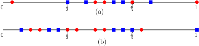
Figure 8: Reduction idea for Claim 23. Here $n=3$. In (a), Alice’s input ${\bf x}=100$ and Bob’s input ${\bf y}=010$; $\textsc{Disj}({\bf x},{\bf y})=1$; $D_{c}^{*}(\mathcal{P})=2$. In (b), ${\bf x}=011$ and ${\bf y}=110$; $\textsc{Disj}({\bf x},{\bf y})=0$; $D_{c}^{*}(\mathcal{P})=3$.

Proof.

We need the following claim where $\mathcal{P}$ be the stream.

Claim 23.

Any one-pass streaming algorithm that outputs an approximate solution $D$ to star-color-discrepancy with probability $\rho$ such that $(1-\epsilon)D_{c}^{*}(\mathcal{P})\leq D\leq 2(1+\epsilon)D_{c}^{*}(\mathcal{P})$, uses $\Omega(n)$ bits of space, where $\mathcal{P}$ is the input stream of length $n$ and $0<\epsilon<\frac{1}{5}$.

Let there exist an algorithm as stated in Theorem 22 that outputs $D^{\prime}$ for color-discrepancy and uses space of $o(n)$ bits. Now using Fact 17, we have $D^{\prime}\leq(1+\epsilon)D_{c}(\mathcal{P})\leq 2(1+\epsilon)D_{c}^{*}(\mathcal{P})$ and $D^{\prime}\geq(1-\epsilon)D_{c}(\mathcal{P})\geq(1-\epsilon)D_{c}^{*}(\mathcal{P})$. So, we can report $D^{\prime}$ as our $D$, i.e., the approximate solution to our star-color-discrepancy satisfying $(1-\epsilon)D_{c}^{*}(\mathcal{P})\leq D\leq 2(1+\epsilon)D_{c}^{*}(\mathcal{P})$. Note that we are using $o(n)$ bits, which contradicts Claim 23. ∎

Remark 2.

Multipass lower bound: Using a similar line of arguemnet of Remark 1, we can have the followings.

• Any $p$-pass algorithm that computes $\epsilon$-multiplicative solution to color-discrepancy (geometric-discrepancy), requires $\Omega\left(\frac{n}{p}\right)$ bits of space, where $0<\epsilon<\frac{1}{5}$.

• Any $p$-pass algorithm that computes $\epsilon$-additive solution to color-discrepancy (geometric-discrepancy), requires $\Omega\left(\frac{1}{\epsilon p}\right)$) bits of space, where $0<\epsilon<1$.

Proof of Claim 23.

We show a reduction from Disj. Let $\mathcal{A}$ be an algorithm that solves correctly star-color-discrepancy, as stated, with probability $2/3$ and uses $o(n)$ bits of space. Now we can design a protocol by suitably placing “red” and “blue” points and looking for separation of discrepancy values to solve Disj. We process each bit of Alice’s input ${\bf x}$ as follows. See Figure 8. If $x_{i}=1$, we give inputs $\frac{i-1}{n}+\frac{1}{7n}$ and $\frac{i}{n}$ labeled as “red” and “blue”, respectively to $\mathcal{A}$. Otherwise, we give points $\frac{i-1}{n}+\frac{2}{7n}$ and $\frac{i}{n}$ labeled as “blue” and “red”, respectively as inputs. We send the current memory status of $\mathcal{A}$ to Bob. Bob processes his input ${\bf y}$ as follows. If $y_{i}=1$, Bob gives four inputs to $\mathcal{A}$: $\frac{i-1}{n}+\frac{3}{7n}$ and $\frac{i-1}{n}+\frac{4}{7n}$ both labeled as “red”; $\frac{i-1}{n}+\frac{5}{7n}$ and $\frac{i-1}{n}+\frac{6}{7n}$ both labeled as “blue”. If $y_{i}=0$, Bob does nothing. As discussed at the begining of this Section, the discrepancy values at the input points only matter. By construction of the input instance of star-color-discrepancy, each point in $\mathcal{P}$ is in one of the forms: $\frac{i-1}{n}+\frac{j}{5n}$ for some $i\in[n],0\leq j\leq 6$. Recall that $I_{p}=[0,p]$. Observe that, $\left|R(I_{p})-B(I_{p})\right|=0$ if $p=\frac{i}{n}$ for some $i$; $\left|R(I_{p})-B(I_{p})\right|=1$ if $p=\frac{i-1}{n}+\frac{1}{7n}$ or $p=\frac{i-1}{n}+\frac{2}{7n}$ for some $i$. Let $J=\{k:y_{k}=1\}$. Only for $i\in J$, we have $I_{p}$ such that $p=\frac{i-1}{n}+\frac{j}{7n}$, where $3\leq j\leq 6$.

Observe that if $x_{j}=1$, then

$$\left|R(I_{p})-B(I_{p})\right| = 2~{}\mbox{for}~{}p=\frac{j-1}{n}+\frac{3}{7n},$$

$$\left|R(I_{p})-B(I_{p})\right| = 3~{}\mbox{for}~{}p=\frac{j-1}{n}+\frac{4}{7n},$$

$$\left|R(I_{p})-B(I_{p})\right| = 2~{}\mbox{for}~{}p=\frac{j-1}{n}+\frac{5}{7n},$$

$$~{}\mbox{ and}\left|R(I_{p})-B(I_{p})\right| = 1~{}\mbox{for}~{}p=\frac{j-1}{n}+\frac{6}{7n}.$$

If $x_{j}=0$, then

$$\left|R(I_{p})-B(I_{p})\right| = 0~{}\mbox{for}~{}p=\frac{j-1}{n}+\frac{3}{7n},$$

$$\left|R(I_{p})-B(I_{p})\right| = 1~{}\mbox{for}~{}p=\frac{j-1}{n}+\frac{4}{7n},$$

$$\left|R(I_{p})-B(I_{p})\right| = 0~{}\mbox{for}~{}p=\frac{j-1}{n}+\frac{5}{7n},$$

$$~{}\mbox{ and}\left|R(I_{p})-B(I_{p})\right| = 1~{}\mbox{for}~{}p=\frac{j-1}{n}+\frac{6}{7n}.$$

If $\textsc{Disj}({\bf x},{\bf y})=0$, there exists an index $i$ such that $x_{i}=y_{i}=1$, then $D_{c}^{*}(\mathcal{P})=3$ and in this case $\mathcal{A}$ returns at least $(1-\epsilon)D_{c}^{*}(\mathcal{P})$, i.e., more than $\frac{12}{5}$. If $\textsc{Disj}({\bf x},{\bf y})=1$, then $D_{c}^{*}(\mathcal{P})=1$ and in this case $\mathcal{A}$ returns at most $2(1+\epsilon)D_{c}^{*}(\mathcal{P})$, i.e., less than $\frac{12}{5}$. Hence, we report $\textsc{Disj}({\bf x},{\bf y})=1$ if and only if $\mathcal{A}$ gives output less than $\frac{12}{5}$. ∎

4.3 Problem COLOR-DISCREPANCY for sorted sequence

By Theorem 22, approximating color-discrepancy needs $\Omega(n)$ bits. But if the stream $\mathcal{P}$ arrives in a sorted order, we can compute $D_{c}(\mathcal{P})$ using $O(1)$ space.

Theorem 24.

color-discrepancy can be solved exactly by a one-pass deterministic streaming algorithm using $O(1)$ space when $\mathcal{P}$ is sorted.

Proof.

Let $I_{opt}=[p,q]$ be an interval where $D_{c}(\mathcal{P})=\left|R(I_{opt})-B(I_{opt})\right|$ is optimized. Then $p,q\in\mathcal{P}$ and $D_{c}(\mathcal{P})\neq 0$, i.e., $R(I_{opt})\neq B(I_{opt})$. Also if $R(I_{opt})>B(I_{opt})$ then $p,q$ are red points and if $R(I_{opt})<B(I_{opt})$ then $p,q$ are blue points. To establish the theorem, we need the following Claim.

Claim 25.

$D_{c}(\mathcal{P})=\max\limits_{p\in\mathcal{P}}\left(R\left([0,p]\right)-B\left([0,p]\right)\right)-\min\limits_{q\in\mathcal{P}}\left(R\left([0,q]\right)-B\left([0,q]\right)\right)+1$.

The algorithm keeps track of the number of red (denoted as $\#R$) and blue (denoted as $\#B$) points seen so far. It also maintains aother two variables — $max$ and $min$. On receiving an input, increment $\#R$ or $\#B$ accordingly and then update $max$ with $\max(max,\#R-\#B)$ and $min$ with $\min(min,\#R-\#B)$. Observe that $D_{c}(\mathcal{P})=max-min+1$ by Claim 25. ∎

Proof of Claim 25.

$$D_{c}(\mathcal{P}) = \max\limits_{I\subset[0,1]}\left|R(I)-B(I)\right|$$

$$= \max\limits_{p,q\in\mathcal{P}}\left|R\left([p,q]\right)-B\left([p,q]\right)\right|$$

$$= \max\Big{(}\max\limits_{p,q\in\mathcal{P},R\left([p,q]\right)>B\left([p,q]\right)}\left(R\left([p,q]\right)-B\left([p,q]\right)\right),$$

$$\quad\quad\quad\quad\quad\quad\max\limits_{p,q\in\mathcal{P},B\left([p,q]\right)>R\left([p,q]\right)}\left(B\left([p,q]\right)-R\left([p,q]\right)\right)\;\;\;\;\Big{)}$$

$$= \max\Big{(}\max\limits_{p,q\in\mathcal{P},R\left([p,q]\right)>B\left([p,q]\right)}\left(\left(R\left([0,q]\right)-R\left([0,p]\right)+1\right)-\left(B\left([0,q]\right)-B\left([0,p]\right)\right)\right),$$

$$\quad\quad\quad\quad\quad\quad\max\limits_{p,q\in\mathcal{P},B\left([p,q]\right)>R\left([p,q]\right)}\left(\left(B\left([0,q]\right)-B\left([0,p]\right)+1\right)-\left(R\left([0,q]\right)-R\left([0,p]\right)\right)\right)\Big{)}$$

$$= \max\limits_{p,q\in\mathcal{P}}\left|(R([0,q])-R([0,p]))-(B([0,q])-B([0,p]))\right|+1$$

$$= \max\limits_{p,q\in\mathcal{P}}\left|(R([0,q])-B([0,q]))-(R([0,p])-B([0,p]))\right|+1$$

$$= \max_{p\in\mathcal{P}}(R([0,p])-B([0,p]))-\min_{q\in\mathcal{P}}(R([0,q])-B([0,q]))+1$$

∎

References

- AC [14] S. Arya and T. M. Chan. Better Epsilon-Dependencies for Offline Approximate Nearest Neighbor Search, Euclidean Minimum Spanning Trees, and Epsilon-Kernels. In SoCG, page 416, 2014.
- AHV [04] P. K. Agarwal, S. Har-Peled, and K. R. Varadarajan. Approximating extent measures of points. J. ACM, 51(4):606–635, 2004.
- AMP+ [06] D Agarwal, A McGregor, J. M. Phillips, S. Venkatasubramanian, and Z. Zhu. Spatial Scan Statistics: Approximations and Performance Study. In KDD, pages 24–33, 2006.
- AMS [99] N. Alon, Y. Matias, and M. Szegedy. The Space Complexity of Approximating the Frequency Moments. J. Comput. Syst. Sci., 58(1):137–147, 1999.
- AN [16] A. Andoni and H. L. Nguyên. Width of Points in the Streaming Model. ACM Trans. Algorithms, 12(1):5, 2016.
- AS [15] P. K. Agarwal and R. Sharathkumar. Streaming Algorithms for Extent Problems in High Dimensions. Algorithmica, 72(1):83–98, 2015.
- BCEG [07] A. Bagchi, A. Chaudhary, D. Eppstein, and M. T. Goodrich. Deterministic sampling and range counting in geometric data streams. ACM Trans. Algorithms, 3(2), 2007.
- BCNS [15] A. Bishnu, A. Chakrabarti, S. C. Nandy, and S. Sen. On Density, Threshold and Emptiness Queries for Intervals in the Streaming Model. In FSTTCS, pages 336–349, 2015.
- Ben [77] J. L. Bently. Algorithms for Klee’s rectangle problem. Unpublished manuscript, 1977.
- BS [80] J. L. Bentley and J. B. Saxe. Decomposable Searching Problems I: Static-to-Dynamic Transformation. J. Algorithms, 1(4):301–358, 1980.
- CC [07] T. M. Chan and E. Y. Chen. Multi-Pass Geometric Algorithms. Discrete & Computational Geometry, 37(1):79–102, 2007.
- Cha [06] T. M. Chan. Faster core-set constructions and data-stream algorithms in fixed dimensions. Comput. Geom., 35(1-2):20–35, 2006.
- Cha [09] T. M. Chan. Dynamic Coresets. Discrete & Computational Geometry, 42(3):469–488, 2009.
- Cha [10] T. M. Chan. A (slightly) faster algorithm for klee’s measure problem. Comput. Geom., 43(3):243–250, 2010.
- Cha [13] T. M. Chan. Klee’s Measure Problem Made Easy. In FOCS, pages 410–419, 2013.
- Cha [16] T. M. Chan. Dynamic Streaming Algorithms for Epsilon-Kernels. In SoCG, pages 27:1–27:11, 2016.
- CP [14] T. M. Chan and V. Pathak. Streaming and dynamic algorithms for minimum enclosing balls in high dimensions. Comput. Geom., 47(2):240–247, 2014.
- CP [15] S. Cabello and P. Pérez-Lantero. Interval Selection in the Streaming Model. In WADS, pages 127–139, 2015.
- Dud [74] R.M Dudley. Metric entropy of some classes of sets with differentiable boundaries. Journal of Approximation Theory, 10(3):227 – 236, 1974.
- EHR [12] Y. Emek, M. M. Halldórsson, and A. Rosén. Space-Constrained Interval Selection. In ICALP, pages 302–313, 2012.
- FIS [08] G. Frahling, P. Indyk, and C. Sohler. Sampling in Dynamic Data Streams and Applications. Int. J. Comput. Geometry Appl., 18(1/2):3–28, 2008.
- FKZ [04] J. Feigenbaum, S. Kannan, and J. Zhang. Computing Diameter in the Streaming and Sliding-Window Models. Algorithmica, 41(1):25–41, 2004.
- FM [85] P. Flajolet and G. N. Martin. Probabilistic Counting Algorithms for Data Base Applications. J. Comput. Syst. Sci., 31(2):182–209, 1985.
- GM [08] S. Guha and A. McGregor. Tight Lower Bounds for Multi-pass Stream Computation Via Pass Elimination. In ICALP, pages 760–772, 2008.
- GM [12] S. Guha and A. McGregor. Graph Synopses, Sketches, and Streams: A Survey. PVLDB, 5(12):2030–2031, 2012.
- HM [04] S. Har-Peled and S. Mazumdar. On coresets for k-means and k-median clustering. In STOC, pages 291–300, 2004.
- HRR [98] M. R. Henzinger, P. Raghavan, and S. Rajagopalan. Computing on Data Streams. In External Memory Algorithms, Proceedings of a DIMACS Workshop, pages 107–118, 1998.
- HS [08] J. Hershberger and S. Suri. Adaptive sampling for geometric problems over data streams. Comput. Geom., 39(3):191–208, 2008.
- Ind [03] P. Indyk. Better Algorithms for High-dimensional Proximity Problems via Asymmetric Embeddings. In SODA, pages 539–545, 2003.
- [30] P. Indyk. Algorithms for Dynamic Geometric Problems over Data Streams. In STOC, pages 373–380, 2004.
- [31] P. Indyk. Streaming Algorithms for Geometric Problems. In FSTTCS, pages 32–34, 2004.
- Kle [77] V. Klee. Can computed in less than steps? Amer. Math. Monthly, 1977.
- KLL [16] Z. S. Karnin, K. J. Lang, and E. Liberty. Optimal Quantile Approximation in Streams. In FOCS, pages 71–78, 2016.
- KN [74] L. Kuipers and H. Niederreiter. Uniform Distribution of Sequences. John Wiley & Sons, 1974.
- KN [97] E. Kushilevtiz and N. Nishan. Communication Complexity. In Cambridge University Press, 1997.
- KNW [10] Daniel M. Kane, Jelani Nelson, and David P. Woodruff. An optimal algorithm for the distinct elements problem. In PODS, pages 41–52, 2010.
- Mat [99] J. Matousek. Geometric Discrepancy: An Illustrated Guide. Springer, 1999.
- Mor [78] R. Morris. Counting Large Numbers of Events in Small Registers. Commun. ACM, 21(10):840–842, 1978.
- MP [78] J. I. Munro and M. S. Paterson. Selection and Sorting with Limited Storage. In FOCS, pages 253–258, 1978.
- Mut [05] S. Muthukrishnan. Data Streams: Algorithms and Applications. FSTTCS, 1(2), 2005.
- OY [91] M. H. Overmars and C.-K. Yap. New Upper Bounds in Klee’s Measure Problem. SIAM J. Comput., 20(6):1034–1045, 1991.
- Rou [16] T. Roughgarden. Communication Complexity (for Algorithm Designers). FSTTCS, 11(3-4):217–404, 2016.
- RR [15] R. A. Rufai and D. S. Richards. A Streaming Algorithm for the Convex Hull. In CCCG, 2015.
- SBV+ [15] G. Sharma, C. Busch, R. Vaidyanathan, Suresh Rai, and J. L. Trahan. Efficient transformations for Klee’s measure problem in the streaming model. Comput. Geom., 48(9):688–702, 2015.
- SLNX [09] A. D. Sarma, A. Lall, D. Nanongkai, and J. Xu. Randomized Multi-pass Streaming Skyline Algorithms. PVLDB, 2(1):85–96, 2009.
- STZ [06] S. Suri, C. D. Tóth, and Y. Zhou. Range Counting over Multidimensional Data Streams. Discrete & Computational Geometry, 36(4):633–655, 2006.
- TW [12] S. Tirthapura and D. P. Woodruff. Rectangle efficient aggregation in spatial data stream. PODS, pages 283–294, 2012.
- vLW [81] J. van Leeuwen and D. Wood. The measure problem for rectangular ranges in d-space. J. Algorithms,2, pages 282–300, 1981.
- Woo [04] D. P. Woodruff. Optimal Space Lower Bounds for all Frequency Moments. In SODA, pages 167–175, 2004.
- Zar [11] H. Zarrabi-Zadeh. An Almost Space-Optimal Streaming Algorithm for Coresets in Fixed Dimensions. Algorithmica, 60(1):46–59, 2011.
- ZC [06] H. Zarrabi-Zadeh and T. M. Chan. A Simple Streaming Algorithm for Minimum Enclosing Balls. In CCCG, 2006.
- Zha [05] Jian Zhang. Massive Data Streams in Graph theory and Computational Geometry. PhD thesis, Yale University, USA, 2005.