Anomalous heat equation in a system connected to thermal reservoirs

Abstract

We study anomalous transport in a one-dimensional system with two conserved quantities in presence of thermal baths. In this system we derive exact expressions of the temperature profile and the two point correlations in steady state as well as in the non-stationary state where the later describe the relaxation to the steady state. In contrast to the Fourier heat equation in the diffusive case, here we show that the evolution of the temperature profile is governed by a non-local anomalous heat equation. We provide numerical verifications of our results.

Transport of energy across an extended system is a paradigm of the vast class of non-equilibrium phenomena. At a macroscopic level this phenomena is often described by the phenomenological Fourier’s law which relates the energy current density $j(x,t)$ to the gradient of the temperature field $T(x,t)$: $j=-\kappa~{}\partial_{x}T$ where $\kappa$ is the thermal conductivity. This law implies diffusive energy flow across the system described by the Fourier heat equation

$$\partial_{\tau}T(x,t)=D~{}\partial_{x}^{2}T(x,t),$$ (1)

where $D=\kappa/c$ (for simplicity we assume $\kappa$ and the specific heat $c$ to be independent of temperature). This equation is widely used in experiments to understand the spreading of local energy perturbations in equilibrium as well as the non-equilibrium dynamics of systems connected to reservoirs.

Surprisingly, several theoretical Narayan2002 ; VanBeijeren2012 ; Spohn2014 , numerical as well as experimental studies Lee2017 suggest that in many one and two dimensional systems heat transfer is anomalous in the sense that Fourier’s law is not valid Lepri2003a ; Dhar2008 ; Lepri2016 . This phenomenon is usually manifested by several interesting features like divergence of thermal conductivity $\kappa$ with system size $L$ as $\kappa\sim L^{\alpha};~{}0<\alpha<1$, power-law decay of the equilibrium current-current auto-correlations, super-diffusive spreading of local energy perturbations, nonlinear stationary temperature profiles (even for small temperature differences) and the presence of boundary singularities in these profiles Dhar2001 ; Dhar2008 ; Lepri2016 ; Narayan2002 ; Lepri1998 ; Liu2014 ; Das2014 ; Bernardin2015 ; Bernardin2012 ; Jara2015 .

There is currently no general framework to describe and explain anomalous heat transport. Recently, the theory of nonlinear fluctuating hydrodynamics has been remarkably successful in predicting anomalous scaling of dynamical correlations of conserved quantities in one-dimensional Hamiltonian systems and the corresponding slow decay of the equilibrium current-current autocorrelations VanBeijeren2012 ; Spohn2014 ; Spohn2016 ; Mendl2015 . This approach provides diverging thermal conductivity (via Green-Kubo formula) as well as Lévy scaling for the spreading of local energy perturbation. On the rigorous side, computations were done for a model of harmonic chain whose Hamiltonian dynamics was supplemented by a stochastic part that kept the conservation laws (number, energy, momentum) intact — we refer to this model as the harmonic chain momentum exchange (HCME) model. For the infinite HCME system it was shown exactly that the current autocorrelation has a $\sim t^{-1/2}$ decay Basile2006a . It was also shown that, in contrast to Eq. (1), the evolution of an initially localized energy perturbation satisfied a non-local fractional diffusion equation $\partial_{t}e(x,t)=-c(-\Delta)^{3/4}e(x,t)$, where $e(x,t)$ is the energy perturbation and $c$ is some constant Bernardin2015 ; Bernardin2012 ; Jara2015 ; Bernardin2016 . The fractional laplacian operator $(-\Delta)^{3/4}$ in the infinite space is defined by its Fourier spectrum: $|q|^{3/2}$ whereas the same for the normal Laplacian operator $-\Delta\equiv-\partial^{2}_{x}$ is $q^{2}$. In real space $(-\Delta)^{3/4}$ operator is non-local fractional1 ; fractional2 .

While all these studies consider transport in isolated systems, quite often the transport set up in an experiment consists of an extended system connected at the two ends to heat baths at different temperatures. For diffusive systems Eq. (1) continues to describe both non-equilibrium steady state (NESS) and time-dependent properties in this set-up. It is then natural to ask: what would be the corresponding evolution equation for the temperature profile in the case of anomalous transport in the experimental set-up? A major problem that now arises follows from the fact that the fractional Laplacian is a non-local operator and so extending its definition to a finite domain is non-trivial. Several studies have addressed this issue, using a phenomenological approach, in the context of Levy walks and Levy flights in finite domains Viswanathan2000 ; Zoia2007 . It is thus crucial to have examples of specific microscopic models of systems exhibiting anomalous transport, for which the time-evolution equation in an open system set up can be derived analytically, and where one can see the non-local and fractional equation forms explicitly. This is the main aim of this Letter.

Such attempts have recently been made in Lepri2009 ; Delfini2008 ; Cividini2017 where the problem of non-linear steady state temperature profiles and their time-evolution in the HCME model was addressed. The specific model studied was a harmonic chain of $N$ particles where, in addition to the Hamiltonian dynamics, the momenta of nearest neighborhood particles is exchanged randomly at a constant rate $\gamma$. The chain is attached to two Langevin baths at the two ends at temperatures $T_{\ell}$ and $T_{r}$. This system has three conserved fields: the stretch $r_{i}=q_{i+1}-q_{i}$ (where $q_{i},~{}i=1,\ldots,N$ are the particle positions) the momentum, $p_{i}$ and the energy $\epsilon_{i}=p_{i}^{2}/2+r_{i}^{2}/2$. This system shows anomalous current behavior $j\sim N^{-1/2}$ as well as exhibits a non-linear stationary temperature profile $T_{i}=\langle p_{i}^{2}/2\rangle_{ss}=\mathcal{T}(i/N)$, which was computed analytically for fixed and free boundary conditions — surprisingly the temperature-profile was different for these cases Lepri2009 ; Cividini2017 . The evolution of the non-stationary temperature profile $\mathcal{T}(x,\tau)$ (where the $\tau=t/N^{3/2}$ is the rescaled time) to the NESS profile was also studied Lepri2010 , where by eliminating the fast variables it was shown that $\mathcal{T}(x,\tau)$ satisfies an energy continuity equation. From an analysis of this equation it was noted that the evolution appears to be similar to the fractional diffusion equation. However, so far this has not been clearly established and in particular an explicit representation of the corresponding fractional evolution operator is not known. In this Letter, we look at a simpler model of anomalous transport in one dimension where we derive the corresponding fractional evolution equation for the temperature profile inside a finite domain and show explicitly how this evolution approaches to the appropriate fractional diffusion operator in the infinite domain.

This model consists of a finite one dimensional lattice of $L$ sites where each site carries a ‘stretch’ variable $\eta_{i},~{}i=1,2,...,L$ under an onsite external potential $V(\eta_{i})=\eta_{i}^{2}/2$. The lattice is attached to two thermal reservoirs at temperatures $T_{\ell}$ and $T_{r}$ on the left and right ends, respectively and subjected to a volume conserving stochastic noise. The dynamics of this model has two parts: (a) the usual deterministic part plus the Langevin terms coming from the baths and (b) a stochastic exchange part where $\eta$s from any two neighboring sites, chosen at random, are exchanged at some rate $\gamma$. The dynamics is given by

$$\begin{split}\frac{d\eta_{i}}{dt}=&~{}V^{\prime}(\eta_{i+1})-V^{\prime}(\eta_{i-1})\\ &+\delta_{i,1}\left(-\lambda V^{\prime}(\eta_{1})+\sqrt{2\lambda T_{\ell}}\zeta_{\ell}(t)\right)\\ &+\delta_{i,L}\left(-\lambda V^{\prime}(\eta_{L})+\sqrt{2\lambda T_{r}}\zeta_{r}(t)\right)\\ &+\text{stochastic~{}exchange~{}at~{}rate~{}}\gamma\end{split}$$ (2)

with fixed boundary conditions (BCs) $\eta_{0}=\eta_{L+1}=0$. Here $\zeta_{\ell,r}(t)$ are mean zero and unit variance, independent Gaussian white noises. Note that, in contrast to the HCME case, this dynamics has two conserved quantities: the ‘volume’ $\eta_{i}$ and the energy $V(\eta_{i})$. This model was first introduced by Bernardin and Stoltz in the closed system setup Bernardin2012 where starting from the harmonic chain with Hamiltonian given earlier, they have treated the positions $q_{i}$s and the momenta $p_{i}$s on the same footing. Note that for harmonic chain, the dynamics of the ‘stretch’ variable $r_{i}=q_{i+1}-q_{i}$ and the momentum variable are similar: $\dot{r}_{i}=p_{i+1}-p_{i}$ and $\dot{p}_{i}=r_{i+1}-r_{i}$ for $i=1,2,...,N$. Hence for $N=L/2$, defining $\eta_{2j-1}=r_{j}$ and $\eta_{2j}=p_{j}$, one finds that both the above equations can be expressed in a single equation: $\dot{\eta}_{m}=\eta_{m+1}-\eta_{m-1}$ for $m=1,2,...,L$. The system can also be interpreted as a fluctuating interface where the algebraic volume of the interface at site $m$ is given by $\eta_{m}$ and the energy $V(\eta)=\eta^{2}/2$ Bernardin2012 . Hence, the stochastic exchange part in Eq. (2) can be thought of as a volume-energy conserving noise. We call this model as ‘harmonic chain with volume exchange’ (HCVE).

It has been shown that the HCVE model defined on an isolated infinite one dimensional lattice (i.e. $\lambda=0$ in Eq. (2) with $i=-\infty,..,-1,0,1,..,\infty$) exhibits super diffusion of energy Bernardin2016 :

$$\begin{split}&\partial_{t}e(x,t)=-\mathbb{L}_{\infty}[e(x,t)],~{}\\ &\mathbb{L}_{\infty}=\frac{1}{\sqrt{2\gamma}}[(-\Delta)^{3/4}-\nabla(-\Delta)^{1/4}],\end{split}$$ (3)

where the skew-fractional operator $\mathbb{L}_{\infty}$ has the Fourier representation $|q|^{3/2}(1-{\mathrm{i}\mkern 1.0mu}~{}\text{sgn}(q))$ with ${\mathrm{i}\mkern 1.0mu}=\sqrt{-1}$ and sgn(q) is the Signum function. In this paper, however, we consider the HCVE model on a finite lattice of size $L$ in open set up i.e. connected to heat baths at the two ends as described in Eq. (2). It is known that in this case also, as in HCME, the stationary current scales as $j\sim L^{-1/2}$ Bernardin2016 .

Results.- We explicitly find that in the large $L$ limit the stationary ‘energy’ current $j_{ss}$ is given, in the leading order, by

$$j_{ss}=\frac{1}{2}\sqrt{\frac{\pi}{\gamma}}~{}\frac{(T_{\ell}-T_{r})}{\sqrt{L}}.$$ (4)

In the non-stationary regime, we numerically find that the temperature profile $T_{i}(t)=\langle V(\eta_{i}(t))\rangle$ and the two-point correlations $C_{i,j}(t)=\langle\eta_{i}(t)\eta_{j}(t)\rangle$ for $i\neq j$ have the following scaling forms

$$\begin{split}T_{i}(t)&=\mathcal{T}\left(\frac{i}{L},\frac{t}{L^{3/2}}\right)\\ C_{i,j}(t)&=\frac{1}{\sqrt{L}}\mathcal{C}\left(\frac{|i-j|}{\sqrt{L}},\frac{i+j}{2L},\frac{t}{L^{3/2}}\right),\end{split}$$ (5)

in the leading order for large $L$. The scaling functions $\mathcal{T}(y,\tau)$ and $\mathcal{C}(x,y,\tau)$ satisfy the following equations inside the domain $\mathcal{D}=\{0\leq x\leq\infty~{};~{}0\leq y\leq~{}1\}$:

$$\partial_{y}\mathcal{C}(x,y,\tau) =-\gamma\partial_{x}^{2}\mathcal{C}(x,y,\tau)$$ (6)

$$\partial_{y}\mathcal{T}(y,\tau) =-2\gamma\left[\partial_{x}\mathcal{C}(x,y,\tau)\right]_{x=0}$$ (7)

$$\partial_{\tau}\mathcal{T}(y,\tau) =2\partial_{y}\mathcal{C}(0,y,\tau),$$ (8)

with $\mathcal{C}(x,y,0)|_{x\to\infty}=0$ and $\mathcal{C}(x,y,0)=0$. We find that the exact solutions of these equations are given by

$$\mathcal{T}(y,\tau) =\mathcal{T}_{ss}(y)+\mathcal{T}_{r}(1-y,\tau)$$ (9)

$$\mathcal{C}(x,y,\tau) =\mathcal{C}_{ss}(x,y)+\mathcal{C}_{r}(x,1-y,\tau).$$ (10)

In the above equation, NESS part of the profiles are

$$\begin{split}\mathcal{T}_{ss}(y)&=T_{r}+(T_{\ell}-T_{r})~{}\sqrt{1-y},\\ \mathcal{C}_{ss}(x,y)&=-\frac{T_{\ell}-T_{r}}{4}\sqrt{\frac{\pi}{\gamma}}~{}\text{erfc}\left(\frac{x}{\sqrt{4\gamma(1-y)}}\right),\end{split}$$ (11)

and the relaxation parts are

$$\mathcal{C}_{r}(x,z,\tau)=-\int_{0}^{z}\frac{\exp\left(-\frac{x^{2}}{4\gamma(z-z^{\prime})}\right)}{\sqrt{4\pi\gamma(z-z^{\prime})}}~{}\frac{\partial\mathcal{T}_{r}(z^{\prime},\tau)}{\partial z^{\prime}}dz^{\prime}$$ (12)

where $\mathcal{T}_{r}(z,\tau)$ satisfies the following continuity equation:

$$\partial_{\tau}\mathcal{T}_{r}(z,\tau)=\frac{1}{\sqrt{\pi\gamma}}\partial_{z}\left[\int_{0}^{z}dz^{\prime}~{}\frac{\partial_{z^{\prime}}\mathcal{T}_{r}(z^{\prime},\tau)}{\sqrt{z-z^{\prime}}}~{}\right],$$ (13)

inside the domain $0\leq z\leq 1$ with BCs $\mathcal{T}_{r}(0,\tau)=\mathcal{T}_{r}(1,\tau)=0$. The relaxation parts $\mathcal{T}_{r}(z,\tau)$ and $\mathcal{C}_{r}(x,z,\tau)$ describe the approach towards the NESS solutions in the $\tau\to\infty$ limit. The equations Eq. (4), Eq. (11), Eq. (12) and Eq. (13), comprise our main results. Note that the evolution of the temperature in Eq. (13) is indeed given by a linear but non-local equation defined inside a finite domain $0~{}\leq~{}z~{}\leq~{}1$. However, following a similar calculation for infinite system we later show that Eq. (13) reduces to Eq. (3) SM . This establishes, without ambiguity, that the non-local operator in Eq. (13) is the correct finite domain representation of the fractional operator $\mathbb{L}_{\infty}$ in Eq. (3). Another point to note that the temperature profile in SS, $\mathcal{T}_{ss}(y)$, is asymmetric under space reversal as the microscopic model itself does not have such symmetry. As a result, any locally created perturbation splits into one traveling sound mode and one non-moving heat mode. This is in contrast to the HCME model where one observes two sound modes moving in opposite directions in addition to a non-moving heat mode Spohn2016 ; Bernardin2012 . Consequently, in this case, there is singularity in $\partial_{y}\mathcal{T}_{ss}(y)$ only at one boundary and we find that the meniscus exponent Lepri2011 is again $1/2$ as in the HCME model with fixed boundary conditions. Interestingly, it turns out that for this boundary condition, both the temperature and the correlation become independent of the strength of coupling $\lambda$ with the heat baths in the large $L$ limit.

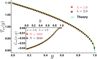
Figure 1: Numerical verification of the analytical NESS predictions for $\mathcal{T}_{ss}(y)$ and $\mathcal{C}_{ss}(x,y)$ in Eq. (11). Symbols are obtained from simulations with $\omega=\gamma=1,~{}T_{\ell}=1.1,~{}T_{r}=0.9$ and $N=1024$, whereas the solid lines are from theory.

Derivation of the results: We start with the Fokker-Planck (FP) equation associated to the dynamics Eq. (2), which describes the evolution of the joint distribution $P(\vec{\eta},t)$ of $\vec{\eta}=(\eta_{1},\eta_{2},\cdots,\eta_{L})$ at time $t$ :

$$\partial_{t}P(\vec{\eta},t) =[\mathcal{L}_{\ell}+\mathcal{L}_{b}+\mathcal{L}_{ex}]~{}P(\vec{\eta},t),$$ (14)

where, $\mathcal{L}_{\ell}$ is the Liouvillian part, $\mathcal{L}_{b}$ contains the effects of the Langevin baths at the boundaries and $\mathcal{L}_{ex}$ represents the contribution from the exchange noise. Explicit expressions of these operators are given in SM . While it is usually hard to compute explicitly the full joint distribution $P(\vec{\eta},t)$, computing various correlations and fluctuations is more tractable and they contain the most useful information about the non-equilibrium state. In this paper, for HCVE model we compute all the two point correlations $\langle\eta_{i}(t)\eta_{j}(t)\rangle$ exactly in the limit of large system size.

Starting from the FP equation in Eq. (14), we obtain the dynamical equations satisfied by $T_{i}=\langle\eta_{i}^{2}(t)\rangle$ and $C_{i,j}=\langle\eta_{i}(t)\eta_{j}(t)\rangle$ for $i\neq j$ in the bulk:

$$\begin{split}&\dot{C}_{ij}=C_{i+1,j}-C_{i-1,j}+C_{i,j+1}-C_{i,j-1}\\ &~{}~{}~{}~{}+\gamma[C_{i-1,j}+C_{i+1,j}+C_{i,j-1}+C_{i,j+1}-4C_{i,j}],\\ &\dot{C}_{i,i+1}=T_{i+1}-C_{i-1,i+1}+C_{i,i+2}-T_{i}\\ &~{}~{}~{}~{}~{}~{}~{}~{}~{}~{}~{}+\gamma[C_{i-1,i+1}+C_{i,i+2}-2C_{i,i+1}],\\ &\dot{T}_{i}=2[C_{i,i+1}-C_{i-1,i}]+\gamma[T_{i+1}+T_{i-1}-2T_{i}].\end{split}$$ (15)

Rest of the equations at the boundaries are given in SM . Fortunately the equations for two point correlations do not involve higher order correlations, this allows us to solve these equations analytically, in the $L\to\infty$ limit.

To proceed we follow the strategy in Lepri2010 . We first solve these equations numerically to observe that, for large $L$ the solutions have the scaling properties as given in Eq. (5) where we have two length scales of $O(L)$ along the diagonal ($i+j=$constant) and of $O(\sqrt{L})$ along perpendicular to the diagonal ($|i-j|=$constant) direction, and a time scale of $O(L^{3/2})$. This time scale can be anticipated from the propagator $e^{-|q|^{3/2}[1-{\mathrm{i}\mkern 1.0mu}\text{sgn}(q)]t}$ of the Eq. (3) in Fourier space. The two length scales are understood by looking at the orders of the $C_{i,j}$ and $T_{i}$, and their derivatives numerically SM . These observations suggest that we look for solutions of Eq. (15) in the scaling form Eq. (5). Inserting these forms in Eq. (15), and expanding in $\epsilon=L^{-1/2}$, we obtain three coupled linear differential equations as given in Eq. (6)-Eq. (8) in the leading order SM . Interestingly, the scaled correlation function $\mathcal{C}$ relaxes very fast over much shorter time scale [$O(L)$] compared to the evolution time scale [$O(L^{3/2})$] of the temperature field $\mathcal{T}$. Due to this fact, Eq. (6) and Eq. (7) do not involve the time derivative. As a result the correlation function $\mathcal{C}$ evolves adiabatically obeying the (anti-)diffusion Eq. (6), with a drive at the boundary by the time dependent temperature field through Eq. (7). The equation for the temperature profile given in Eq. (8) is in the expected continuity equation.

In the NESS the equations (6)-(8) become simpler since $\partial_{\tau}\mathcal{T}\to 0$ as $\tau\to\infty$ implying $\mathcal{C}_{ss}(0,y)=d$. Now making the variable transformation $z=(1-y)$, the problem of finding $\mathcal{C}_{ss}$ reduces to solving a diffusion equation with its value at $x=0$ held fixed for all $y$. It is easy to show that the solution is given by $\mathcal{C}_{ss}(x,y)=d~{}\text{erfc}(x/\sqrt{4\gamma(1-y)})$ where $\text{erfc}(v)$ is the complementary error function SM . Now inserting this solution in Eq. (7) and solving with boundary conditions $\mathcal{T}_{ss}(0)=T_{\ell}$ and $\mathcal{T}_{ss}(1)=T_{r}$, we get the explicit expression Eq. (11). In Fig. 1 we verify the analytical results for $T_{ss}$ and $\mathcal{C}_{ss}$ numerically, where we observe nice agreement. One can easily identify the microscopic current from the equation for $\dot{T}_{i}$ in Eq. (15) as $j=-2C_{i,i+1}-\gamma(T_{i+1}-T_{i})$ which in the steady state for large $L$ provides $j_{ss}=-2\mathcal{C}_{ss}(0,y)/\sqrt{L}$. Note that the term $-\gamma(T_{i+1}-T_{i})$ contributes at $\mathcal{O}(1/L)$. Now inserting the expression of $\mathcal{C}_{ss}(0,y)$ from Eq. (11), one obtains the expression for $j_{ss}$ given in Eq. (4).

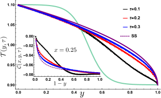
Figure 2: Numerical verification of the evolution of the temperature profiles $\mathcal{T}(y,\tau)=\mathcal{T}_{ss}(y)+\mathcal{T}_{r}(1-y,\tau)$ obtained using the solution of Eq. (13). Inset shows the verification of the correlation $\mathcal{C}(x,y,\tau)=\mathcal{C}_{ss}(x,y)+\mathcal{C}_{r}(x,1-y,\tau)$ given in Eq. (10) where $\mathcal{C}_{r}$ is computed using the solution in Eq. (12). The green line and the dashed purple line represent the initial and the NESS temperature profiles, respectively. Symbols are obtained from simulations with $\lambda=\gamma=1,~{}T_{\ell}=1.1,~{}T_{r}=0.9$ and $L=2048$, and the solid lines are from theory.

We now focus on the relaxation to the NESS. It is often convenient to separate the relaxation part as done in Eq. (9) and Eq. (10) where $\mathcal{T}_{r}(z,\tau)$ and $\mathcal{C}_{r}(x,z,\tau)$ describes the approach towards the NESS solutions in Eq. (11). It is easy to see that $\mathcal{C}_{r}(x,z,\tau)$ and $\mathcal{T}_{r}(z,\tau)$ satisfies the following equations

$$\partial_{z}\mathcal{C}_{r}(x,z,\tau) =\gamma\partial_{x}^{2}\mathcal{C}_{r}(x,z,\tau),$$ (16)

$$\partial_{z}\mathcal{T}_{r}(z,\tau) =2\gamma\left[\partial_{x}\mathcal{C}_{r}(x,z,\tau)\right]_{x=0},$$ (17)

$$\partial_{\tau}\mathcal{T}_{r}(z,\tau) =-2\partial_{z}\mathcal{C}_{r}(0,z,\tau),$$ (18)

with initial condition $\mathcal{C}_{r}(x,z,0)=0$ and BC $\mathcal{C}_{r}(x,z,\tau)|_{x\to\infty}=0$. The above equations are obtained from Eq. (6)-(8) after subtracting the steady state part and then making the variable transformation $z=(1-y)$. Note that the BC in Eq. (17) acts like a current source, at $x=0$ boundary, to the diffusion Eq. (16). It is easy to show SM that the solution of this equation is given precisely by Eq. (12). Now, inserting this solution in Eq. (18) and performing some simplifications we arrive at the non-local evolution Eq. (13) (see SM ) with boundary conditions $\mathcal{T}_{r}(0,\tau)=\mathcal{T}_{r}(1,\tau)=0$. Hence it is natural to expand the solution in $\sin$ basis $\alpha_{n}(z)=\sqrt{2}~{}\sin(n\pi z)$, $n=1,2,...$: $\mathcal{T}_{r}(z,\tau)=\sum_{n=1}^{\infty}\hat{\mathcal{T}}_{r}(n,\tau)~{}\alpha_{n}(z)$ for all $\tau\geq 0$. Inserting this form in Eq. (13) and simplifying we find that the coefficients $\hat{\mathcal{T}}_{r}(n,\tau)$ satisfy the following matrix equation

$$\frac{d\hat{\mathcal{T}}_{r}}{d\tau}=\kappa{\bf B}~{}\hat{\mathcal{T}}_{r},$$ (19)

where ${\bf B}$ is an infinite order matrix with elements ${\bf B}_{m,n}$ specified in SM and $\kappa=1/\sqrt{\pi\gamma}$. While it is difficult to solve this infinite order matrix equation analytically, we solve it numerically by truncating it at some finite order. In Fig. 2, we compare the evolution from this numerical solution with the same obtained from direct numerical simulation of Eq. (2) and observe nice agreement. Using this solution in Eq. (12) we obtain $C(x,z,\tau)$ in Eq. (10) which we also compare with simulation results in the inset of Fig. 2 and again observe good agreement.

From the numerical solution of Eq. (19) we, in addition, observe that the eigenvalues obtained , are in general complex and are of the form $\lambda_{n}\approx|n\pi|^{3/2}(1-{\mathrm{i}\mkern 1.0mu}\text{sgn})$, for large $n>0$, while at small values of $n$ the eigenvalues deviate from this behaviour SM . We confirm that this is not due to the the truncation of the matrix but an artefact of the finiteness of the system. Note that the large $n$ behavior of $\lambda_{n}$ is similar to the Fourier spectrum of the non-local operator $\mathbb{L}_{\infty}$ in Eq. (3) describing the evolution in infinite system. Hence it is interesting to see if one recovers the evolution Eq. (3) in the infinite system limit. One can follow the same calculation procedure on an infinite lattice as presented before for finite lattice and arrive at an evolution equation for temperature profile similar to Eq. (13) with only difference being that the lower limit of the integral on the rhs is $-\infty$, as the equation is now valid in $-\infty\leq y\leq\infty$. Now taking Fourier transform on both sides it is quite easy to show that the evolution equation in infinite space indeed reduces to the skew-fractional equation in Eq. (3). A more direct and detailed proof is given in SM .

Conclusion: In this Letter, we have studied anomalous transport in a one-dimensional system with two conserved quantities, in the open system setup. Starting from a microscopic description and acquiring knowledge about scaling properties from numerical studies, we derive exact expressions of the temperature profiles and the two point correlations in the steady state. We also study the evolution of these quantities towards steady state. We explicitly show that the evolution of the temperature profiles in this model is governed by a non-local operator defined inside a finite domain which correctly takes the previously obtained infinite system representation. We provide numerical verifications of the analytical results. Our work provides the first clear and transparent microscopic derivation of non-local heat equation describing anomalous transport in finite geometry and its connection to the corresponding skew-fractional equation in the infinite domain.

We thank C. Bernardin, C. Mejía-Monasterio, S. Olla and S. Lepri for very useful discussions. AK acknowledges support from DST grant under project No. ECR/2017/000634.

I Dynamical operators and Discrete equations

The explicit expression of the deterministic part of the Fokker Planck (FP) equation given by operators ${\cal{L}}_{l}$, ${\cal{L}}_{b}$, defined as

$${\cal L}_{l} =\sum_{i=1}^{L-1}(V^{\prime}(\eta_{i+1})-V^{\prime}(\eta_{i-1}))\partial_{\eta_{i}}-V^{\prime}(\eta_{L-1})\partial_{\eta_{L}}+V^{\prime}(\eta_{2})\partial_{\eta_{1}}$$

$${\cal L}_{b} =\lambda T_{\ell}~{}\partial^{2}_{\eta_{1}}-\lambda\partial_{\eta_{1}}V^{\prime}(\eta_{1})+\lambda T_{r}~{}\partial^{2}_{\eta_{L}}-\lambda\partial_{\eta_{L}}V^{\prime}(\eta_{L}),$$

where $T_{\ell}$ and $T_{r}$ are the temperatures of the reservoirs on the left and right, respectively. The stochastic part ${\cal{L}}_{ex}$ is given as

$${\cal L}_{ex}=\gamma\left(\sum_{i=1}^{L-1}P(\vec{\eta}_{i,i+1})-P(\vec{\eta})\right)$$ (S1)

where $\vec{\eta}_{i,i+1}$ denote the configuration after the exchange of variable $i$ with $i+1$. The two point function defined as, $C_{i,j}=\langle\eta_{i}\eta_{j}\rangle$. From the above FP equation for $V(\eta)=\eta^{2}/2$, the dynamical equation $C_{i,j}=\langle\eta_{i}\eta_{j}\rangle$s can easily be written as

$$\dot{C}_{ij}~{} =C_{i+1,j}-C_{i-1,j}+C_{i,j+1}-C_{i,j-1}+\gamma[C_{i-1,j}+C_{i+1,j}+C_{i,j-1}+C_{i,j+1}-4C_{i,j}],~{}~{}1<i,j<L$$ (S2)

$$\dot{C}_{i,i+1}~{} =T_{i+1}-C_{i-1,i+1}+C_{i,i+2}-T_{i}+\gamma[C_{i-1,i+1}+C_{i,i+2}-2C_{i,i+1}],~{}~{}1<i<L$$ (S3)

$$\dot{T}_{i}~{} =2[C_{i,i+1}-C_{i-1,i}]+\gamma[T_{i+1}+T_{i-1}-2T_{i}],~{}~{}1\leq i\leq L$$ (S4)

The dynamical equations at the boundaries are given by

• for $i=j=1$

  $$\dot{T}_{1}=2\lambda T_{\ell}+2C_{1,2}-2\lambda T_{1}+\gamma[T_{2}-T_{1}]$$ (S5)

• for $i=j=L$

  $$\dot{T}_{L}=2\lambda T_{r}-2C_{L-1,L}-2\lambda T_{L}+\gamma[T_{L-1}-T_{L}]$$ (S6)

• $i=1$ and $1<j<L$

  $$\dot{C}_{1,j}=C_{2,j}-\lambda C_{1,j}+C_{1,j+1}-C_{1,j-1}+\gamma[C_{1,j-1}+C_{1,j+1}+C_{2,j}-3C_{1,j}]$$ (S7)

• $j=L$ and $1<i<L$

  $$\dot{C}_{i,L}=C_{i+1,L}-C_{i-1,L}-C_{i,L-1}-\lambda C_{i,L}+\gamma[C_{i-1,L}+C_{i+1,L}+C_{i,L-1}-3C_{i,L}]$$ (S8)

• $i=1$ and $j=L$

  $$\dot{C}_{1,L}=C_{2,L}-C_{1,L-1}-2\lambda C_{1,L}+\gamma[C_{2,L}+C_{1,L-1}-2C_{1,L}]$$ (S9)

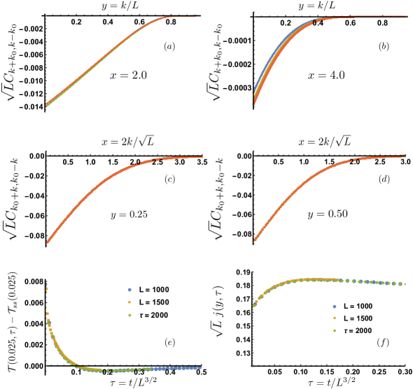
Figure S1: Data collapse of the correlation functions and temperature profile confirming the scaling behaviors in Eqs. (S10) and (S11). Figures (a) and (b) show the data collapse as a function of the scaling variable $y=(i+j)/2L$ with four systems sizes $L=1000$ (Blue), $L=2000$ (Orange), $L=3000$ (Green) and $L=4000$ (Red), for two fixed values of $x=|j-i|/\sqrt{L}$. Figures (c) and (d), show the data collapse as a function of the scaling variable $x$ with the above four system sizes for two fixed values of $y$. The collapse are so good that other colors not visible. Figure (e) describes the scaling behavior for the evolution of the temperature $\mathcal{T}(y,\tau)=T_{\lfloor yL\rfloor}(\tau L^{3/2})$ at a fixed position $y=0.025$ for different system sizes as a function of the scaled time $\tau=t/L^{3/2}$. Note that, the temperatures are of $\mathcal{O}(1)$ whereas the correlations are of $\mathcal{O}(1/\sqrt{L})$. Also note from figures (c) and (b) that $\mathcal{C}_{ss}(x\to\infty,z)=0$. Last figure (d) establishes that the current in the system is of order $1/\sqrt{L}$ and also evolves in scaled time $\tau=t/L^{3/2}$. The other parameters in the simulation are $\gamma=\Lambda=1$, $T_{\ell}=1.1,~{}T_{r}=0.9$.

II Derivation of continuum equations from discrete equations

Now, we want to get a continuum description of the bulk discrete dynamical equations derived in the previous section. In the non-stationary regime, we numerically find that the temperature profile $T_{i}(t)=\langle\eta_{i}(t)^{2}\rangle$ and the two-point correlations $C_{i,j}(t)=\langle\eta_{i}(t)\eta_{j}(t)\rangle$ for $i\neq j$ have the following scaling forms

$$C_{i,j}(t) =\frac{1}{\sqrt{L}}\mathcal{C}\left(\frac{|i-j|}{\sqrt{L}},\frac{i+j}{2L},\frac{t}{L^{3/2}}\right),$$ (S10)

$$T_{i}(t) =\mathcal{T}\left(\frac{i}{L},\frac{t}{L^{3/2}}\right),$$ (S11)

in the leading order for large $L$ which are also supported by numerical evidence shown in Fig S1. In figs. (S1a), (S1b,  (S1c) and  (S1d), verify the scaling behaviors of the correlations in Eq. (S10). Figures (S1c) and  (S1d), describes scaling behavior with respect to time. Using these, we define continuum ordinates as, $\frac{|i-j|}{\sqrt{L}}=x$, $\frac{|i+j|}{2L}=y$, $\frac{t}{L^{3/2}}=\tau$ and $\frac{1}{\sqrt{L}}=\epsilon$, where $x\in(0,\infty)$ and $y\in(0,1)$. In the following, we insert this scaling form and Taylor expand in $\epsilon=1/\sqrt{L}$. Keeping terms to leading order in $\epsilon$ we obtain the continuum equations.

1. Bulk Equations, $|i-j|\geq 2$
   We start with the discrete equation in bulk:

   $$\dot{C}_{i,j}=-\left(C_{i-1,j}-C_{i+1,j}+C_{i,j-1}-C_{i,j+1}-\gamma[C_{i,j-1}+C_{i,j+1}+C_{i+1,j}+C_{i-1,j}-4C_{i,j}]\right),$$ (S12)

   using above scaling definitions, we can write the above mentioned discrete equation as,

   $$\epsilon^{4}\partial_{\tau}\mathcal{C}(x,y,\tau)=-\epsilon\left({\cal C}(x-\epsilon,y-\frac{\epsilon^{2}}{2})-{\cal C}(x+\epsilon,y+\frac{\epsilon^{2}}{2})+{\cal C}(x+\epsilon,y-\frac{\epsilon^{2}}{2})-{\cal C}(x-\epsilon,y+\frac{\epsilon^{2}}{2})\right.$$

   $$\left.-\gamma\left[{\cal C}(x+\epsilon,y-\frac{\epsilon^{2}}{2})+{\cal C}(x-\epsilon,y+\frac{\epsilon^{2}}{2})+{\cal C}(x+\epsilon,y+\frac{\epsilon^{2}}{2})+{\cal C}(x-\epsilon,y-\frac{\epsilon^{2}}{2})-4{\cal C}(x,y)\right]\right)~{},$$ (S13)

   which by Taylor expansion of each terms in $x,~{}y$ and $\tau$, we obtain the leading order terms for continuum dynamical equation as

   $$\epsilon^{4}\partial_{\tau}\mathcal{C}(x,y,\tau)=2\epsilon^{3}\partial_{y}\mathcal{C}(x,y,\tau)+2\gamma\epsilon^{3}\partial^{2}_{x}\mathcal{C}(x,y,\tau)~{}.$$ (S14)

   At the dominant order ($o(\epsilon^{3})$), we find,

   $$\partial_{y}\mathcal{C}(x,y,\tau)+\gamma\partial^{2}_{x}\mathcal{C}(x,y,\tau)=0$$ (S15)

2. Nearest neighbor term, $j=i+1$
   

   $$\dot{C}_{i,i+1}=T_{i+1}-C_{i-1,i+1}+C_{i,i+2}-T_{i}+\gamma\left[C_{i-1,i+1}+C_{i,i+2}-2C_{i,i+1}\right]$$ (S16)

   after proper scaling, we get,

   $$\epsilon^{4}\partial_{\tau}\mathcal{C}(\epsilon,y+\frac{\epsilon^{2}}{2},\tau)={\cal T}(y+\epsilon^{2})-{\cal T}(y)-\epsilon{\cal C}(2\epsilon,y+\epsilon^{2})+\epsilon{\cal C}(2\epsilon,y)+\gamma\epsilon\left[{\cal C}(2\epsilon,y)+{\cal C}(2\epsilon,y+\epsilon^{2})-2{\cal C}(\epsilon,y+\frac{\epsilon^{2}}{2})\right]~{}.$$ (S17)

   Expanding above equation in $x$ and $y$, and keeping the relevant order terms in $\epsilon$ we get the continuum equation as

   $$\epsilon^{4}\partial_{\tau}\mathcal{C}(0,y,\tau)=\epsilon^{2}\left(\partial_{y}\mathcal{T}(y,\tau)+2\gamma\partial_{x}\mathcal{C}(0,y,\tau)\right)+O(\epsilon^{3})$$ (S18)

   and hence to the dominating order, the governing continuum equation is

   $$\partial_{y}\mathcal{T}(y,\tau)+2\gamma\partial_{x}\mathcal{C}(0,y,\tau)=0$$ (S19)

3. Diagonal term $i=j$
   Next is the diagonal term where $i=j$,

   $$\dot{T}_{i}~{} =2[C_{i,i+1}-C_{i-1,i}]+\gamma[T_{i+1}+T_{i-1}-2T_{i}].$$ (S20)

   this in continuum limit given as

   $$\epsilon^{3}\partial_{\tau}\mathcal{T}(y,\tau)=2\epsilon\left[\mathcal{C}(\epsilon,y+\frac{\epsilon^{2}}{2})-\mathcal{C}(\epsilon,y-\frac{\epsilon^{2}}{2})\right]+\gamma\left[\mathcal{T}(y+\epsilon^{2})+\mathcal{T}(y-\epsilon^{2})-2\mathcal{T}(y)\right]$$ (S21)

   After expansion, we arrive at

   $$\epsilon^{3}\partial_{\tau}\mathcal{T}(y,\tau)=2\epsilon\left[\epsilon^{2}\partial_{y}\mathcal{C}(0,y,\tau)+\epsilon^{3}\frac{\gamma}{4}\partial_{y}^{2}\mathcal{T}(y,\tau)\right]+O(\epsilon^{4})$$ (S22)

   Hence, the leading order term is

   $$\partial_{\tau}\mathcal{T}(y,\tau)=2\partial_{y}\mathcal{C}(0,y,\tau)$$ (S23)

4. Current
   The microscopic energy current in the system is defined through

   $$\partial_{t}\langle\eta_{i}^{2}\rangle=-[j_{i\to i+1}-j_{i-1\to i}],$$ (S24)

   where $j_{i\to i+1}=-2C_{i,i+1}-\gamma(T_{i+1}-T_{i})$. The stochastic part of the current decays as $O(1/L)$ and in the macroscopic limit goes to zero. In the continuum limit, the deterministic part contributes in the leading order to provide, $j=-2\mathcal{C}(0,y,\tau)/\sqrt{L}.$

III Solution in the steady state as well as in the relaxation regime

The above analysis gives us the following bulk equations for the system,

$$\partial_{y}\mathcal{C}(x,y,\tau) =-\gamma\partial_{x}^{2}\mathcal{C}(x,y,\tau)~{},$$ (S25)

$$\partial_{y}\mathcal{T}(y,\tau) =-2\gamma\partial_{x}\mathcal{C}(x,y,\tau)_{x=0}~{}$$ (S26)

$$\partial_{\tau}\mathcal{T}(y,\tau) =2\partial_{y}\mathcal{C}(0,y,\tau)$$ (S27)

Solutions of these equations for $\mathcal{C}(x,y,\tau)$ and $\mathcal{T}(y,\tau)$ have two parts. One part describes the steady state and the other part describing the relaxation to the steady state:

$$\mathcal{T}(y,\tau) =\mathcal{T}_{ss}(y)+\mathcal{T}_{r}(1-y,\tau)$$ (S28)

$$\mathcal{C}(x,y,\tau) =\mathcal{C}_{ss}(x,y)+\mathcal{C}_{r}(x,1-y,\tau).$$ (S29)

It is easy to show that $\mathcal{C}_{ss}(x,z)$ and $\mathcal{T}_{ss}(z)$ satisfy

$$\partial_{z}\mathcal{C}_{ss}(x,z) =\gamma\partial_{x}^{2}\mathcal{C}_{ss}(x,z)~{},$$ (S30)

$$\partial_{z}{\cal T}_{ss}(z) =2\gamma\partial_{x}\mathcal{C}_{ss}(x,z)_{x=0}.$$ (S31)

under the transformation of $z=1-y$ with boundary conditions $\mathcal{C}_{ss}(x\to\infty,z)=0,~{}\mathcal{T}_{ss}(0)=T_{\ell}$ and $\mathcal{T}_{ss}(1)=T_{r}$. On the other hand, the relaxation parts satisfy

$$\partial_{z}\mathcal{C}_{r}(x,z,\tau) =\gamma\partial_{x}^{2}\mathcal{C}_{r}(x,z,\tau)~{},$$ (S32)

$$\partial_{z}\mathcal{T}_{r}(z,\tau) =2\gamma\partial_{x}\mathcal{C}_{r}(x,z,\tau)_{x=0}~{}$$ (S33)

$$\partial_{\tau}\mathcal{T}_{r}(y,\tau) =-2\partial_{z}\mathcal{C}_{r}(0,z,\tau).$$ (S34)

with appropriate boundary conditions specified in Sec.III.2.

III.1 Stationary state solution

In stationary state, we first solve Eq. (S30) and Eq. (S31). We want to solve these equations along with the boundary conditions

$$(i)~{}\mathcal{C}_{ss}(x,z\to 0)=0,~{}~{}(ii)~{}\mathcal{C}_{ss}(x\to\infty,z)=0,~{}~{}(iii)~{}\mathcal{C}_{ss}(x=0,z)=d.$$ (S35)

The initial condition in (i) is easy to understand. The boundary condition (ii) is obtained from our numerical observation [see fig. S1(c,d) ]. Where the last boundary condition (iii) is obtained by observing that LHS of (S34) is zero in steady state; hence ($\partial_{z}\mathcal{C}_{ss}(0,z)=0$). The unknown constant $d$ will be fixed by the temperatures at the boundary. The first equation is easy to solve by taking Laplace transform in $z$ along with boundary conditions. Finally inverting the Laplace transform, we find, the solution is given by,

$$\mathcal{C}_{ss}(x,z) =d~{}\text{erfc}\left[\frac{x}{\sqrt{4\gamma z}}\right]$$ (S36)

where, erfc is the complimentary error function defined as $\text{erfc}(x)=1-\frac{2}{\sqrt{\pi}}\int_{0}^{x}dte^{-t^{2}}$. Now, using this solution in the Eq. S31, we get

$$\partial_{z}\mathcal{T}_{ss}(z)= -d~{}\sqrt{\frac{4\gamma}{\pi z}}$$

$${\cal T}_{ss}(z)= {\cal T}_{ss}(0)-2d~{}\sqrt{\frac{4\gamma z}{\pi}}$$ (S37)

The constants ${\cal T}_{ss}(0)$ and $d$ will now be determined from the boundary conditions of temperature field, $\mathcal{T}(z=0)=T_{r}$ and $\mathcal{T}(z=1)=T_{\ell}$,. We finally have,

$$T_{\ell}-T_{r}= ~{}-2d~{}\sqrt{\frac{4\gamma}{\pi}}~{}$$

$$d~{}= ~{}-\frac{\Delta T}{4}\sqrt{\frac{\pi}{\gamma}}~{},$$ (S38)

where $\Delta T=(T_{\ell}-T_{r})$ is the temperature difference between the left and right heat baths. Reverting now back to $y$ variables using $z=1-y$, the exact expressions for the steady state temperature profile and correlations are,

$$\mathcal{T}_{ss}(y)= T_{r}+\Delta T\sqrt{1-y},$$ (S39)

$$\mathcal{C}_{ss}(x,y)= -\frac{\Delta T}{4}\sqrt{\frac{\pi}{\gamma}}\text{erfc}\left[\frac{x}{\sqrt{4\gamma(1-y)}}\right]$$ (S40)

Hence the current in the system is given by $j_{ss}=\frac{\mathcal{J}_{ss}}{\sqrt{L}}$, where,

$$j_{ss}= -\frac{2\mathcal{C}_{ss}(0,y)}{\sqrt{L}}=\frac{\Delta T}{2}\sqrt{\frac{\pi}{\gamma}}~{}\frac{1}{\sqrt{L}}$$ (S42)

III.2 Solution in the relaxation regime

Here we solve Eqs. (S32), (S33) and (S34) (Note that these are also Eqs. (16),(17) and (18) of the main text). For convenience, we rewrite these equations here,

$$\partial_{z}\mathcal{C}_{r}(x,z,\tau) =\gamma\partial_{x}^{2}\mathcal{C}_{r}(x,z,\tau),$$ (S43)

$$\partial_{z}\mathcal{T}_{r}(z,\tau) =2\gamma\left[\partial_{x}\mathcal{C}_{r}(x,z,\tau)\right]_{x=0},$$ (S44)

$$\partial_{\tau}\mathcal{T}_{r}(z,\tau) =-2\partial_{z}\mathcal{C}_{r}(0,z,\tau).$$ (S45)

We want to solve (S43) with boundary conditions $\mathcal{C}_{r}(x,z)|_{x\to\infty}=0$ and (S44). The Greens function $g(x,z)$ of this equation with above BC’s satisfies, $\partial_{z}g(x,z)=\frac{\gamma}{2}\partial_{x}^{2}g(x,z)$, where, $g(x,z)$ is given by $g(x,z)=\sqrt{4\gamma z}h(x/\sqrt{4\gamma z})$ where, $h(w)=\frac{e^{-w^{2}}}{\pi}-w~{}\text{erfc}(w)$, hence, the general time dependent solution is written as,

$$\mathcal{C}_{r}(x,z,\tau)=2\int_{0}^{z}dx^{\prime}\frac{e^{-(x-x^{\prime})^{2}/(4\gamma z)}}{\sqrt{4\pi\gamma z}}\mathcal{C}_{r}(x^{\prime},0,\tau) -\frac{1}{2\gamma}\left(\int_{0}^{z}dz^{\prime}(g(x,z-z^{\prime})\partial_{z^{\prime}}^{2}\mathcal{T}_{r}(z^{\prime},\tau))\right)$$ (S46)

$$~{}~{}-\frac{1}{2\gamma}~{}\partial_{z^{\prime}}\mathcal{T}_{r}(z^{\prime},\tau)g(x,z)|_{z^{\prime}\to 0}$$

With the initial condition $\mathcal{C}_{r}(x,0,\tau)=0$ the first term drops out. It is easy to check that the remaining part satisfies (16) with boundary condition (17) as follows,

$$\partial_{x}\mathcal{C}_{r}(x,z,\tau)|_{x\to 0}= ~{}-\frac{1}{2\gamma}\left(\int_{0}^{z}dz^{\prime}\partial_{x}g(x,z-z^{\prime}))\partial_{z^{\prime}}^{2}\mathcal{T}_{r}(z^{\prime},\tau)+\partial_{x}g(x,z))\partial_{z^{\prime}}\mathcal{T}_{r}(z^{\prime},\tau)|_{z^{\prime}\to 0}\right)$$

$$= \frac{1}{2\gamma}\left(\int_{0}^{z}dz^{\prime}\partial_{z^{\prime}}^{2}\mathcal{T}_{r}(z^{\prime},\tau)+\partial_{z^{\prime}}\mathcal{T}_{r}(z^{\prime},\tau)|_{z^{\prime}\to 0}\right)=~{}\frac{1}{2\gamma}\partial_{z}\mathcal{T}_{r}(z,\tau)$$ (S47)

where we have used $\partial_{x}g(x,z)|_{x\to 0}=-1$. Further using the fact that $g(x,z-z^{\prime})\partial_{z^{\prime}}T_{r}(z^{\prime})|_{z^{\prime}\to z}\to 0$ we can simplify (S46) as,

$$\mathcal{C}_{r}(x,z,\tau)= -\frac{1}{2\gamma}\left(\int_{0}^{z}dz^{\prime}g(x,z-z^{\prime})\partial_{z^{\prime}}^{2}\mathcal{T}_{r}(z^{\prime},\tau)+\partial_{z^{\prime}}\mathcal{T}_{r}(z^{\prime},\tau)g(x,z)|_{z^{\prime}\to 0}-g(x,z-z^{\prime})\partial_{z^{\prime}}\mathcal{T}_{r}(z^{\prime},\tau)|_{z^{\prime}\to z}\right)$$

$$= ~{}\frac{1}{2\gamma}\left(\int_{0}^{z}dz^{\prime}\partial_{z^{\prime}}(g(x,z-z^{\prime}))\partial_{z^{\prime}}\mathcal{T}_{r}(z^{\prime},\tau)\right)$$

$$= ~{}-\frac{1}{\sqrt{\gamma}}\int_{0}^{z}dz^{\prime}\frac{e^{-x^{2}/(4\gamma(z-z^{\prime}))}}{\sqrt{4\pi(z-z^{\prime})}}\partial_{z^{\prime}}\mathcal{T}_{r}(z^{\prime},\tau)$$ (S48)

which gives the relaxation of the correlation fields. The evolution of temperature field is obtained from (18) by putting $x\to 0$ in the above expression for $\mathcal{C}_{r}(x,z,\tau)$, we immediately have,

$$\partial_{\tau}\mathcal{T}_{r}(z,\tau)=~{}\kappa~{}\partial_{z}\int_{0}^{z}\frac{\partial_{z^{\prime}}\mathcal{T}_{r}(z^{\prime},\tau)}{\sqrt{z-z^{\prime}}}dz^{\prime},~{}~{}0\leq z\leq 1,~{}~{}\text{where},~{}~{}\kappa=\frac{1}{\sqrt{\pi\gamma}}.$$ (S49)

For infinite system, one can perform the same procedure as done above for finite system using appropriate control parameter and obtain

$$\partial_{\tau}\mathcal{T}_{r}(z,\tau)=~{}\kappa~{}\partial_{z}\int_{-\infty}^{z}\frac{\partial_{z^{\prime}}\mathcal{T}_{r}(z^{\prime},\tau)}{\sqrt{z-z^{\prime}}}dz^{\prime},~{}~{}-\infty\leq z\leq\infty.$$ (S50)

III.3 Fractional evolution of temperature in an infinite line

In the previous section we have derived an equation for evolution of temperature the field in an finite system where $y\in(0,1)$. One can extend the same calculation in an finite system of length $L$ and obtain the same set of bulk equations which now hold for $y\in[0,L]$. We are interested in the behavior of the evolution of temperature profile in $L\to\infty$ limit, where the effect of boundaries are not important. The evolution equations for the relaxation parts in this case are,

$$\gamma\partial_{x}^{2}\mathcal{C}_{r}(x,y,\tau) =-\partial_{y}\mathcal{C}_{r}(x,y,\tau)$$

$$\partial_{y}\mathcal{T}_{r}(y,\tau) =-2\gamma\partial_{x}\mathcal{C}_{r}(x,y,\tau)|_{x\to 0}$$ (S51)

$$\partial_{\tau}\mathcal{T}_{r}(y,\tau) =~{}2\partial_{y}\mathcal{C}_{r}(0,y,\tau)$$

where $0\leq x\leq\infty$ and $0\leq y\leq L$. To proceed, we introduce the orthonormal and complete basis in $y\in[0,L]$ , $\phi^{\pm}_{n}(y)=\frac{1}{\sqrt{L}}e^{\pm{\mathrm{i}\mkern 1.0mu}n\pi y/L}$ for $n\geq 1$ and $\phi_{0}(y)=1/\sqrt{L}$. Expanding the correlations and temperature in this basis as Fourier series we get,

$$\mathcal{C}_{r}(x,y,\tau)=\hat{A}_{0}(x,\tau)+\sum_{n=1}\hat{A}^{+}_{n}(x,\tau)\phi^{+}_{n}(y)+\hat{A}^{-}_{n}(x,\tau)\phi^{-}_{n}(y)$$

$$\mathcal{T}(y,\tau)=\hat{T}_{0}(\tau)+\sum_{n=1}\hat{T}^{+}_{n}(\tau)\phi^{+}_{n}(y)+\hat{T}^{-}_{n}(\tau)\phi^{-}_{n}(y)$$ (S52)

where $\hat{A}_{n}^{\pm}(x,\tau)=\int_{0}^{L}\mathcal{C}_{r}(x,y,\tau)\phi_{n}^{\pm}(y)dy$, $\hat{A}_{0}(x,\tau)=\int_{0}^{L}\mathcal{C}_{r}(x,y,\tau)\phi_{0}dy$, $\hat{T}_{n}^{\pm}(\tau)=\int_{0}^{L}\mathcal{T}_{r}(y,\tau)\phi_{n}^{\pm}(y)dy$, $\hat{T}_{0}(\tau)=\int_{0}^{L}\mathcal{T}_{r}(y,\tau)\phi_{0}dy$. These gives the following differential equations for the components,

$$\partial^{2}_{x}\hat{A}^{\pm}_{n}(x,\tau)= ((1\mp{\mathrm{i}\mkern 1.0mu})\alpha_{n})^{2}\hat{A}^{\pm}_{n}(x,\tau),~{}\partial^{2}_{x}\hat{A}_{0}(x,\tau)=0$$ (S53)

$$\pm\frac{{\mathrm{i}\mkern 1.0mu}n\pi}{L}\hat{T}^{\pm}_{n}(\tau)= -2\gamma\partial_{x}\hat{A}^{\pm}_{n}(x,\tau)_{|x\to 0}.$$ (S54)

where $\alpha_{n}=\sqrt{\frac{n\pi}{2L\gamma}}$. The solution to these equations are in general given as,

$$\hat{A}^{\pm}_{n}(x,\tau)= a^{\pm}_{n}(\tau)e^{\pm\alpha_{n}(1\mp{\mathrm{i}\mkern 1.0mu})x},~{}\hat{A}_{0}(x,\tau)=d(\tau)x+e(\tau)$$

We choose solutions which do not blow up at infinity at large $x$ and obey the boundary conditions. We have,

$$\mathcal{C}_{r}(x,y,\tau)= e(\tau)+\sum_{n=1}^{\infty}a_{n}^{-}e^{-\alpha_{n}(1+{\mathrm{i}\mkern 1.0mu})x}\phi_{n}^{-}(y)+c.c.$$ (S55)

where c.c. stands for complex conjugate. $e(\tau)$ is zero because there is no time-dependent source in the system. Using above equations, , we get,

$$\hat{T}^{\pm}_{n}=2\gamma a_{n}^{\mp}(\tau)\alpha_{n}\frac{(1\mp{\mathrm{i}\mkern 1.0mu})}{(n\pi/L)},~{}\dot{\hat{T}}^{\mp}_{n}=\mp 2{\mathrm{i}\mkern 1.0mu}\frac{n\pi}{L}a_{n}^{\pm}(\tau)$$ (S56)

Upon combining these two, we get $\dot{\hat{T}}_{0}=0$ and

$$\dot{\hat{T}}^{\mp}_{n} =-\frac{1}{\sqrt{2\gamma}}(1\pm{\mathrm{i}\mkern 1.0mu})\lambda_{n}^{3/4}\hat{T}^{\mp}_{n},~{}~{}n=1,2,3...$$ (S57)

where $\lambda_{n}=(n\pi/L)^{2}$. This can be interpreted in domain $y\in[0,L]$ as,

$$\partial_{\tau}\mathcal{T}_{r}(y,\tau)=-\frac{1}{\sqrt{2\gamma}}(|\Delta|^{3/4}-\nabla|\Delta|^{1/4})\mathcal{T}_{r}(y,\tau)=-\frac{1}{\sqrt{2\gamma}}\mathbb{L}\mathcal{T}_{r}(y,\tau)$$ (S58)

where $\mathbb{L}$ is an positive operator defined by its action as, $\mathbb{L}\phi_{n}^{\pm}(y)=\lambda^{3/4}_{n}(1-{\mathrm{i}\mkern 1.0mu}~{}\text{sgn}(n))\phi_{n}^{\pm}(y)$. With $L\to\infty$ the spectrum becomes continuous as well as the eigenfunctions become plane wave. Thus in infinite system at equilibrium, the evolution of temperature profile is given by a skew-symmetric fractional Laplacian given in Eq.(3) of the main text.

One can alternatively see this equivalence from the integro-differential evolution in infinite space given in Eq. (S50). Let us write this equation as

$$\partial_{\tau}\mathcal{T}_{r}(y,\tau)=\mathcal{L}_{\infty}\mathcal{T}_{r}(y,\tau),~{}\text{where},~{}\mathcal{L}_{\infty}f(y)=\frac{1}{\sqrt{\pi\gamma}}~{}\partial_{y}\int_{-\infty}^{y}\frac{\partial_{y^{\prime}}f(y^{\prime})}{\sqrt{y-y^{\prime}}}dy^{\prime}.$$ (S59)

Using the identity

$$\int_{-\infty}^{y}dz\frac{1}{\sqrt{y-z}}~{}e^{{\mathrm{i}\mkern 1.0mu}qz}=\frac{\sqrt{\pi}}{\sqrt{{\mathrm{i}\mkern 1.0mu}q}}~{}e^{{\mathrm{i}\mkern 1.0mu}qy}$$

one can easily show that

$$\mathcal{L}_{\infty}~{}e^{{\mathrm{i}\mkern 1.0mu}qy}=\lambda_{q}~{}e^{{\mathrm{i}\mkern 1.0mu}qy},~{}~{}\lambda_{q}=\sqrt{\frac{1}{2\gamma}}[1-{\mathrm{i}\mkern 1.0mu}~{}\text{sgn}(q)]~{}|q|^{3/2}$$

which is same as the Fourier spectrum of the skew-symmetric fractional Laplacian given in Eq.(3) of the main text.

III.4 Series solution of the Fractional PDE in finite domain

The evolution of the relaxation part of the temperature profile i.e. $\mathcal{T}_{r}(1-y,\tau)=\mathcal{T}(y,\tau)-\mathcal{T}_{ss}(y)$ is given by Eq. (S49). Note that, $\mathcal{T}_{r}(z,\tau)$ is zero at both the boundaries: $z=0$ and $z=1$. As a result it natural to expand this function in $\alpha_{n}(z)=\sqrt{2}\sin(n\pi z),~{}n=1,2,3...$ complete basis defined in $z\in(0,1)$, as $\mathcal{T}_{r}(z,\tau)=\sum_{n}\hat{\theta}_{n}(\tau)\alpha_{n}(z)$. Substituting this form in Eq. (S49), we have,

$$\sum_{n}\dot{\hat{\theta}}_{n}\alpha_{n}(z)=\kappa~{}\sum_{n}\hat{\theta}_{n}(\tau)(n\pi)\partial_{z}\int_{0}^{z}\frac{\phi_{n}(z^{\prime})}{\sqrt{z-z^{\prime}}}dz^{\prime}$$ (S60)

Now let us expand the function $f_{n}(z)=\partial_{z}\int_{0}^{z}\frac{\phi_{n}(z^{\prime})}{\sqrt{z-z^{\prime}}}dz^{\prime}$ also in orthogonal basis $\alpha_{n}(y),~{}n=1,2....$. Let the expansion is given as $f_{n}(z)=\sum_{l=1}\zeta_{nl}\alpha_{l}(z)$ where $\zeta_{nl}=\int_{0}^{1}dz~{}f_{n}(z)~{}\alpha_{l}(z)$. As a result we have,

$$\sum_{n=1}\dot{\hat{\theta}}_{n}\alpha_{n}(z)=\kappa~{}\sum_{n,l=1}\hat{\theta}_{n}(\tau)(n\pi)\zeta_{nl}\alpha_{l}(z)$$ (S61)

Using orthogonality, this can be written in vector notation as ($\hat{\theta}_{n}=\langle\;n\;|\;\hat{\theta}\;\rangle$),

$$|\;\dot{\hat{\theta}}\;\rangle=\kappa~{}\mathbf{B}|\;\hat{\theta}\;\rangle,$$ (S62)

where $B_{nk}=(n\pi)\zeta_{nk}$. If $R$ is the matrix which diagonalizes $\mathbf{B}$ as $R^{-1}\mathbf{B}R=\Lambda$, then the time dependent solution is given as $|\;\hat{\theta}(\tau)\;\rangle=Re^{\kappa\Lambda\tau}R^{-1}|\;\hat{\theta}(0)\;\rangle$ and temperature at time $\tau$ is given as $\mathcal{T}(y,\tau)=\mathcal{T}_{ss}(y)+\langle\;\alpha(1-y)\;|\;\hat{\theta}(\tau)\;\rangle$. The eigenvalues of the bounded skew-fractional laplacian, $\mathbf{B}$ have interesting behavior, the first four of them are real and distinct. The higher eigenvalues all come in complex conjugate pairs of form $\mu_{n}(1\pm{\mathrm{i}\mkern 1.0mu})$. For large $n$, $\mu_{n}$ goes as $\sqrt{\frac{\pi}{2}}(n\pi)^{3/2}$, but for smaller $n$ there is a systematic deviation due to the effect of finite domain. In Fig. S2, the real part of alternate eigenvalues are plotted as a function of $n$, where the asymptotic scaling with $\sqrt{\frac{\pi}{2}}(n\pi)^{3/2}$ is seen clearly for large $n$. The eigenvectors of the operator is defined as $\psi_{n}(y)=\sum_{l=1}R^{-1}_{nl}\alpha_{l}(y)$. Numerically computing this gives, the first six eigenvectors to be completely real. The eigenvectors corresponding to higher eigenvalues are complex and and comes in pairs. The real and imaginary parts of the first few eigenvectors are shown in Fig.S3(a). In Fig.S3(b), the real and the imaginary part of the eigenvector for $n\geq 7$ is plotted in polar plots. For plane wave solutions these would have been circles of length 1, here the polar plot shows a spiral decay to origin owing to the skewness of the operator.

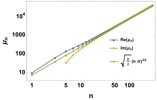
Figure S2: The real and imaginary part of the alternate eigenvalues for the matrix B. The first $4$ eigenvalues are completely real and distinct. The higher eigenvalue comes in pairs of $\mu_{n}(1\pm{\mathrm{i}\mkern 1.0mu})$. For large $n$, the eigenvalues are close to $\sqrt{\frac{\pi}{2}}(n\pi)^{3/2}(1\pm{\mathrm{i}\mkern 1.0mu})$. For smaller $n$, there is a deviation from asymptomatic scaling.

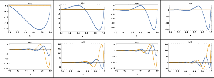
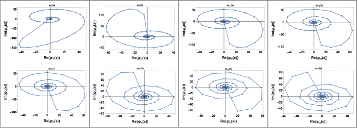
Figure S3: (a)The real (Blue) and Imaginary (Orange) part of the right eigenvectors for the matrix B for the first few eigenvalues. (b) Polar plots showing the real and imaginary parts of the eigenvectors for $n\geq 7$. The polar plots are for $n=7,9,11...$. The plots for even ordered eigenvectors ($N=8,10...$) are related to the eigenvectors of the previous eigenvectors by a reflection around x axis and hence are not plotted.

As the temperature field evolves at much faster timescales compared to the correlation field, the time dependent solution for correlations $\mathcal{C}_{r}(x,1-y,\tau)$ is governed by the evolution of the temperature field. The solution for evolution of correlations is written as, $\mathcal{C}(x,y,\tau)=\mathcal{C}_{r}(x,1-y,\tau)+\mathcal{C}_{ss}(x,y)$ , where,

$$\mathcal{C}(x,z,\tau)= -\int_{0}^{z}dz^{\prime}\frac{e^{-x^{2}/(4\gamma(z-z^{\prime}))}}{\sqrt{4\pi\gamma(z-z^{\prime})}}\partial_{z^{\prime}}T_{r}(z^{\prime},\tau)$$

$$= \sum_{n=1}\hat{\theta}_{n}(\tau)(n\pi)\int_{0}^{z}dz^{\prime}\frac{e^{-x^{2}/(4\gamma(z-z^{\prime}))}}{\sqrt{4\pi\gamma(z-z^{\prime})}}\phi_{n}(z^{\prime})$$ (S63)

where, $\phi_{n}(y)=\sqrt{2}\cos(n\pi y),~{}n\geq 1$ and $\phi_{0}(y)=1$. The integral can be evaluated explicitely and doing the summations gives the evolution of the correlation fields.

References

[1]
Onuttom Narayan and Sriram Ramaswamy.
Anomalous Heat Conduction in One-Dimensional Momentum-Conserving
Systems.
Physical Review Letters, 89(20), 2002.
[2]
Henk Van Beijeren.
Exact results for anomalous transport in one-dimensional hamiltonian
systems.
Physical Review Letters, 108(18), 2012.
[3]
Herbert Spohn.
Nonlinear Fluctuating Hydrodynamics for Anharmonic Chains.
Journal of Statistical Physics, 154(5):1191–1227, feb 2014.
[4]
Victor Lee, Chi Hsun Wu, Zong Xing Lou, Wei Li Lee, and Chih Wei Chang.
Divergent and Ultrahigh Thermal Conductivity in Millimeter-Long
Nanotubes.
Physical Review Letters, 118(13), 2017.
[5]
Stefano Lepri, Roberto Livi, and Antonio Politi.
Universality of anomalous one-dimensional heat conductivity.
Physical Review E - Statistical Physics, Plasmas, Fluids, and
Related Interdisciplinary Topics, 68(6), 2003.
[6]
Abhishek Dhar.
Heat transport in low-dimensional systems.
Advances in Physics, 57(5):457–537, 2008.
[7]
Stefano Lepri, Roberto Livi, and Antonio Politi.
Heat transport in low dimensions: Introduction and phenomenology.
Lecture Notes in Physics, 921:1–37, 2016.
[8]
Abhishek Dhar.
Heat conduction in a one-dimensional gas of elastically colliding
particles of unequal masses.
Physical Review Letters, 86(16):3554–3557, 2001.
[9]
S. Lepri, R. Livi, and A. Politi.
On the anomalous thermal conductivity of one-dimensional lattices.
Europhysics Letters, 43(3):271–276, 1998.
[10]
Sha Liu, Peter Hänggi, Nianbei Li, Jie Ren, and Baowen Li.
Anomalous heat diffusion.
Physical Review Letters, 112(4), 2014.
[11]
Suman G. Das, Abhishek Dhar, Keiji Saito, Christian B. Mendl, and Herbert
Spohn.
Numerical test of hydrodynamic fluctuation theory in the
Fermi-Pasta-Ulam chain.
Physical Review E - Statistical, Nonlinear, and Soft Matter
Physics, 90(1), 2014.
[12]
Cédric Bernardin, Patrícia Gonçalves, Milton Jara, Makiko
Sasada, and Marielle Simon.
From Normal Diffusion to Superdiffusion of Energy in the Evanescent
Flip Noise Limit.
Journal of Statistical Physics, 159(6):1327–1368, 2015.
[13]
Cédric Bernardin and Gabriel Stoltz.
Anomalous diffusion for a class of systems with two conserved
quantities.
Nonlinearity, 25(4):1099–1133, 2012.
[14]
Milton Jara, Tomasz Komorowski, and Stefano Olla.
Superdiffusion of Energy in a Chain of Harmonic Oscillators with
Noise.
Communications in Mathematical Physics, 339(2):407–453, 2015.
[15]
Herbert Spohn.
Fluctuating hydrodynamics approach to equilibrium time correlations
for anharmonic chains.
Lecture Notes in Physics, 921:107–158, 2016.
[16]
Christian B. Mendl and Herbert Spohn.
Current fluctuations for anharmonic chains in thermal equilibrium.
Journal of Statistical Mechanics: Theory and Experiment,
2015(3), 2015.
[17]
Giada Basile, Cédric Bernardin, and Stefano Olla.
Momentum conserving model with anomalous thermal conductivity in low
dimensional systems.
Physical Review Letters, 96(20), 2006.
[18]
Cédric Bernardin, Patrícia Gonçalves, and Milton Jara.
3/4-Fractional Superdiffusion in a System of Harmonic Oscillators
Perturbed by a Conservative Noise.
Archive for Rational Mechanics and Analysis, 220(2):505–542,
2016.
[21]
G. M. Viswanathan, V. Afanasyev, Sergey V. Buldyrev, Shlomo Havlin, M. G.E. Da
Luz, E. P. Raposo, and H. Eugene Stanley.
Levy flights in random searches.
Physica A: Statistical Mechanics and its Applications,
282(1):1–12, 2000.
[22]
A. Zoia, A. Rosso, and M. Kardar.
Fractional Laplacian in bounded domains.
Physical Review E - Statistical, Nonlinear, and Soft Matter
Physics, 76(2), 2007.
[23]
S. Lepri, C. Mejía-Monasterio, and A. Politi.
A stochastic model of anomalous heat transport: Analytical solution
of the steady state.
Journal of Physics A: Mathematical and Theoretical, 42(2),
2009.
[24]
Luca Delfini, Stefano Lepri, Roberto Livi, and Antonio Politi.
Nonequilibrium invariant measure under heat flow.
Physical Review Letters, 101(12), 2008.
[25]
J. Cividini, A. Kundu, A. Miron, and D. Mukamel.
Temperature profile and boundary conditions in an anomalous heat
transport model.
Journal of Statistical Mechanics: Theory and Experiment,
2017(1), 2017.
[26]
Stefano Lepri, Carlos Mejía-Monasterio, and Antonio Politi.
Nonequilibrium dynamics of a stochastic model of anomalous heat
transport.
Journal of Physics A: Mathematical and Theoretical, 43(6),
2010.
[27]
Supplementary Material .
[28]
Stefano Lepri and Antonio Politi.
Density profiles in open superdiffusive systems.
Physical Review E - Statistical, Nonlinear, and Soft Matter
Physics, 83(3), 2011.
Supplementary Material: Anomalous heat equation in a system connected to thermal reservoirs
1International Centre for Theoretical Sciences, Tata Institute of Fundamental Research,
Bengaluru 560089, India