Cosmological Tests With Strong Gravitational Lenses using Gaussian Processes

Abstract

Strong gravitational lenses provide source/lens distance ratios $\mathcal{D}_{\rm obs}$ useful in cosmological tests. Previously, a catalog of 69 such systems was used in a one-on-one comparison between the standard model, $\Lambda$CDM, and the $R_{\rm h}=ct$ universe, which has thus far been favored by the application of model selection tools to many other kinds of data. But in that work, the use of model parametric fits to the observations could not easily distinguish between these two cosmologies, in part due to the limited measurement precision. Here, we instead use recently developed methods based on Gaussian Processes (GP), in which $\mathcal{D}_{\rm obs}$ may be reconstructed directly from the data without assuming any parametric form. This approach not only smooths out the reconstructed function representing the data, but also reduces the size of the $1\sigma$ confidence regions, thereby providing greater power to discern between different models. With the current sample size, we show that analyzing strong lenses with a GP approach can definitely improve the model comparisons, producing probability differences in the range $\sim 10-30\%$. These results are still marginal, however, given the relatively small sample. Nonetheless, we conclude that the probability of $R_{\rm h}=ct$ being the correct cosmology is somewhat higher than that of $\Lambda$CDM, with a degree of significance that grows with the number of sources in the subsamples we consider. Future surveys will significantly grow the catalog of strong lenses and will therefore benefit considerably from the GP method we describe here. In addition, we point out that if the $R_{\rm h}=ct$ universe is eventually shown to be the correct cosmology, the lack of free parameters in the study of strong lenses should provide a remarkably powerful tool for uncovering the mass structure in lensing galaxies.

1 Introduction

The degree to which light from high-redshift quasars is deflected by intervening galaxies can be calculated precisely if one has enough information concerning the distribution of mass within the gravitational lens 1 ; 2 . Depending on the mass of the galaxy, and the alignment between source, lens, and observer, gravitational lenses may be classified either as macro (with sub-classes of strong and weak lensing) or micro lensing systems. Strong lensing occurs when the source, lens, and observer are sufficiently well aligned that the deflection of light forms an Einstein ring. Using the angle of deflection, one may derive the radius of this ring, from which one may then also compute the angular diameter distance to the lens. This distance, however, is model dependent. Hence, together with the measured redshift of the source, this angular diameter distance may be used to discriminate between various cosmological models (see, e.g., ref. 3 ; 4 ; 5 ; 6 ; 7 ).

In this paper, we use a recent compilation of 118 8 plus 40 9 strong lensing systems, with good spectroscopic measurements of the central velocity dispersion based on the SLACS (Sloan Lens ACS) Survey 4 ; 10 ; 11 , and the LSD (Lenses Structure and Dynamics) Survey (see, e.g., refs. 12 ; 13 ), to conduct a comparative study between $\Lambda$CDM 14 ; 15 and another Friedmann-Robertson-Walker (FRW) cosmology known as the $R_{\rm h}=ct$ universe 16 ; 17 . Over the past decade, such comparative tests between this alternative model and $\Lambda$CDM have been carried out using a wide assortment of data, most of them favouring the former over the latter (for a summary of these tests, see Table 1 in ref. 18 ). These studies have included high $z$-quasars 19 , gamma-ray bursts 15 , Type Ia SNe 21 ; 22 , and cosmic chronometers 23 . The $R_{\rm h}=ct$ model is characterized by a total equation of state $p=-\rho/3$, in terms of the total pressure $p$ and density $\rho$ in the cosmic fluid.

The results of these comparative tests are not yet universally accepted, however, and several counterclaims have been made in recent years. One may loosely group these into four general categories: (1) that the gravitational radius (and therefore also the Hubble radius) $R_{\rm h}$ is not really physically meaningful 24 ; 25 ; 26 ; (2) that the zero active mass condition $\rho+3p=0$ at the basis of the $R_{\rm h}=ct$ cosmology is inconsistent with the actual constitutents in the cosmic fluid 27 ; (3) that the $H(z)$ data favour $\Lambda$CDM over $R_{\rm h}=ct$ 25 ; 28 ; and (4) that Type Ia SNe also favour the concordance model over $R_{\rm h}=ct$ 25 ; 28 ; 29 . These works, and papers published in response to them 17 ; 23 ; 30 ; 31 ; 32 ; 33 , have generated an important discussion concerning the viability of $R_{\rm h}=ct$ that we aim to continue here. In § 7 below, we will discuss at greater length the need to use truly model-independent data in these tests, basing their analysis on sound statistical practices. Such due diligence is of utmost importance in any serious attempt to compare different cosmologies in an unbiased fashion.

The test most directly relevant to the work reported here was carried out using strong lenses by ref. 7 , who based their comparison on parametric fits from the models themselves, and concluded that both cosmologies account for the data rather well. The precision of the measurements used in that application, however, was not good enough to favour either model over the other. In this paper, we revisit that sample of strong lensing systems and use an entirely different approach for the comparison, based on Gaussian Processes (GP) to reconstruct the function representing the data non-parametrically. In so doing, the angular diameter distance to the lensing galaxies is determined without pre-assuming any model, providing a better comparison of the competing cosmologies using a functional area minimization statistic described in § 6. An obvious benefit of this approach is that a reconstructed function representing the data may be found regardless of whether or not any of the models being tested is actually the correct cosmology.

In § 2 of this paper, we describe the lensing equation used in cosmological tests, and we then describe the data used with this application in § 3. The Gaussian processes are summarized in § 4, and in § 5 we describe the cosmological models being tested here. The area minimization statistic is introduced in § 6, and we explain how this is used to obtain the model probabilities. We end with our conclusions in § 7.

2 Theory of Lensing

In work with strong lensing, the observed images are typically fitted using a singular isothermal ellipsoid approximation (SIE) for the lens 34 . The projected mass distribution at redshift $z_{l}$ is assumed to be elliptical, with semi-major axis $\theta_{2}$ and semi-minor axis $\theta_{1}$. Often, an even simpler approximation suffices, and we make use of it in this paper: we use a singular isothermal sphere (SIS) for the lens model, in which the semi-major and semi-minor axes are equal, i.e., $\theta_{1}=\theta_{2}$. To provide context for this approach, we first describe SIE lens model and afterwards restrict it further by setting $\theta_{1}=\theta_{2}$. The lens equation 35 that relates the position $\beta$ in the source plane to the position $\theta$ in the image plane is given by

$$\beta=\theta-\nabla_{\theta}\Phi\;,$$ (1)

where $\Phi$ is the lensing potential of the SIE given as 36

$$\Phi=\theta_{\rm E}\sqrt{(1-\epsilon)\,\theta_{1}^{2}+(1+\epsilon)\,\theta_{2}^{2}}\;,$$ (2)

and $\epsilon$ is the ellipticity related to the eccentricity according to

$$e=\sqrt{\frac{1-\epsilon}{1+\epsilon}}\;.$$ (3)

In Equation (2), $\theta_{\rm E}$ is the Einstein radius, defined as

$$\theta_{\rm E}=4\pi\left(\frac{\sigma_{v}}{c}\right)^{2}\mathcal{D}\;,$$ (4)

where $\sigma_{v}$ is the velocity dispersion within the lens and

$$\mathcal{D}\equiv\frac{D_{A}(z_{l},z_{s})}{D_{A}(0,z_{s})}\;.$$ (5)

Notice that Equation (4) is independent of the Hubble constant $H_{0}$. Nonetheless, one must still measure $\sigma_{v}$, the total velocity dispersion of stellar and dark matter. Obtaining this quantity is challenging because it is not the average line-of-sight velocity dispersion weighted with surface-brightness. The velocity dispersion of the SIS ($\sigma_{SIS}$ or $\sigma_{v})$, may be related to the central velocity dispersion $\sigma_{0}$, which is obtained from the stellar velocity dispersion with one-eighth the effective optical radius (see, e.g., refs. 4 ; 5 ). Though this works quite well for massive elliptical galaxies, which are indistinguishable kinematically from an SIE within one effective radius, $\sigma_{SIS}$ and $\sigma_{0}$ are actually not equal. Dark matter is dynamically hotter than bright stars so the velocity dispersion of the former must be greater than that of the latter 37 . Treu et al. 4 studied the homogeneity of early-type galaxies using the large samples of lenses identified by the Sloan Lenses ACS Survey (SLACS; 10 ; 38 ) and found that $f_{SIS}\equiv\langle{\sigma_{SIS}}/{\sigma_{0}}\rangle=1.010\pm 0.017$ when fitting the geometry of multiple images. Similar results were found in ref. 39 , who examined the ratio of stellar velocity dispersion to $\sigma_{SIS}$ for different anisotropy parameters. The accumulation of evidence therefore suggests that $f_{SIS}=1.01$, and this is the value we adopt for this study. Thus, following ref. 40 , we write the Einstein Radius as

$$\theta_{\rm E}=4\pi\left(\frac{\sigma_{SIS}}{c}\right)^{2}\mathcal{D}\;,$$ (6)

where

$$\sigma_{SIS}=f_{SIS}\,\sigma_{0}\;.$$ (7)

The data based on Equation (6) will be used to compare our two cosmological models in this paper. The errors associated with individual measurements of $\mathcal{D}$ are calculated from the error propagation equation,

$$\sigma_{\mathcal{D}}=\mathcal{D}_{\rm obs}\left[\left(\frac{\sigma_{\theta_{\rm E}}}{\theta_{\rm E}}\right)^{2}+4\left(\frac{\sigma_{\sigma_{0}}}{\sigma_{0}}\right)^{2}+4\left(\frac{\sigma_{f}}{f_{SIS}}\right)^{2}\right]^{1/2}\;,$$ (8)

containing $\theta_{\rm E}$, $\sigma_{0}$, $f_{SIS}=1.01$ and $\sigma_{f}=0.017$. We follow Grillo et al. 5 and set $\sigma_{\theta_{\rm E}}=0.05\,\theta_{\rm E}$ and $\sigma_{\sigma_{0}}=0.05\,\sigma_{0}$. The overall dispersion in $\mathcal{D}$ is expected to be $\sigma_{\mathcal{D}}\sim 0.11\mathcal{D}_{\rm obs}$.

3 Data

The compilation we use here contains 158 strong lensing systems. These have excellent spectroscopic measurements of the central velocity dispersion, obtained using the Sloan Lens ACS (SLACS) Survey 4 ; 10 ; 11 and the LSD (Lenses Structure and Dynamics) survey 12 ; 13 . One can also find some of the original contributions to these datasets in refs. 41 ; 42 ; 43 ; 44 ; 45 ; 46 ; 47 ; 48 . The velocity dispersion (and its aforementioned error $\sim 5$%) are obtained from SDSS (Sloan Digital Sky Survey Database).

Table 1. Strong Gravitational Lensing Systems with $0.45<z_{s}<0.475$

Galaxy	$z_{l}$	$\theta_{\rm E}$	$\sigma_{0}$	$\mathcal{D}_{\rm obs}$	$\sigma_{\mathcal{D}}$	$\mathcal{D}_{R_{\rm h}=ct}$	$\mathcal{D}_{\Lambda{\rm CDM}}$	Refs.a
		(arc sec)	(km s-1)	$f_{SIS}$=1.010
SDSS J1134 + 6027	0.1528	1.10	$239\pm 12$	0.6689	0.735	0.634	0.652	10
SDSS J1403 + 0006	0.1888	0.83	$213\pm 17$	0.635	0.069	0.553	0.573	10
SDSS J2300 + 0022	0.2285	1.25	$305\pm 19$	0.446	0.0512	0.460	0.479	1-9
SDSS J0956 + 5100	0.2405	1.32	$318\pm 17$	0.4536	0.0498	0.441	0.459	1-9
SDSS J0935 - 0003	0.3475	0.87	$396\pm 35$	0.192	0.0211	0.222	0.234	10,11

^aReference: (1) 50 ; (2) 46 ; (3) 49 ; (4) 47 ; (5) 48 ; (6) 4 ; (7) 11 ; (8) 5 ; (9) 6 ; (10) 12 ; (11) 13

Given that two distances are involved for each lens-source pairing, the GP method calls for a reconstruction of $\mathcal{D}(z_{l},z_{s})$ in two dimensions. This will only be feasible, however, when the sample is large enough to yield enough statistics to warrant this full approach. For now, even with 158 strong lensing systems, we are constrained to consider small redshift ranges, effectively reducing the problem to a one-dimensional reconstruction in each sub-division. Because the data are less dispersed in the lens plane, where $0.1<z_{l}<0.5$, and scattered much more in the source plane, $0.3<z_{s}<3.0$, we carry out the reconstruction within thin redshift-shells of sources, turning $D_{\rm obs}(z_{l},z_{s})$ into a one-dimensional function of $z_{l}$ for what is essentially a fixed $z_{s}$. To minimize the scatter in source redshifts, we use a bin size less than 0.025 and choose those bins that have at least 5 data points within them, allowing us to reconstruct $D_{\rm obs}(z_{l},z_{s})$ using GP for each of the selected bins. In our sample of 158 strong-lensing systems, these criteria therefore allow us to assemble 5 different redshift bins, with anywhere from 5 to 9 lens-source pairs in each of them. These strong lenses are displayed in Tables 1 to 5. Note that for the purpose of GP reconstruction in one dimension, we assume that all the sources in redshift bin $(z_{s},z_{s}+\Delta z)$ have the same average redshift $z_{s}+\Delta z/2$.

Table 2. Strong Gravitational Lensing Systems with $0.46<z_{s}<0.485$

Galaxy	$z_{l}$	$\theta_{\rm E}$	$\sigma_{0}$	$\mathcal{D}_{\rm obs}$	$\sigma_{\mathcal{D}}$	$\mathcal{D}_{R_{\rm h}=ct}$	$\mathcal{D}_{\Lambda{\rm CDM}}$	Refs.b
		(arc sec)	(km s-1)	$f_{SIS}$=1.010
SDSS J1134 + 6027	0.1528	1.10	$239\pm 12$	0.6689	0.735	0.634	0.652	10
SDSS J1403 + 0006	0.1888	0.83	$213\pm 17$	0.635	0.069	0.553	0.573	10
SDSS J1402 + 6321	0.2046	1.39	$290\pm 16$	0.5743	0.063	0.526	0.546	1-9
SDSS J1205 + 4910	0.2150	1.22	$281\pm 14$	0.5368	0.059	0.504	0.524	10
SDSS J2300 + 0022	0.2285	1.25	$305\pm 19$	0.446	0.0512	0.460	0.479	1-9
SDSS J0956 + 5100	0.2405	1.32	$318\pm 17$	0.4536	0.0498	0.441	0.459	1-9
SDSS J0935 - 0003	0.3475	0.87	$396\pm 35$	0.192	0.0211	0.222	0.234	10,11

^aReference: (1) 50 ; (2) 46 ; (3) 49 ; (4) 47 ; (5) 48 ; (6) 4 ; (7) 11 ; (8) 5 ; (9) 6 ; (10) 12 ; (11) 13

Table 3. Strong Gravitational Lensing Systems with $0.5<z_{s}<0.525$

Galaxy	$z_{l}$	$\theta_{\rm E}$	$\sigma_{0}$	$\mathcal{D}_{\rm obs}$	$\sigma_{\mathcal{D}}$	$\mathcal{D}_{R_{\rm h}=ct}$	$\mathcal{D}_{\Lambda{\rm CDM}}$	Refs.c
		(arc sec)	(km s-1)	$f_{SIS}$=1.010
SDSS J1451 - 0239	0.1254	1.04	$223\pm 14$	0.726	0.079	0.718	0.735	10,11
SDSS J2303 + 1422	0.1553	1.64	$271\pm 16$	0.775	0.0852	0.654	0.673	1-9
SDSS J1627 - 0053	0.2076	1.21	$295\pm 13$	0.482	0.052	0.552	0.573	1-9
SDSS J1142 + 1001	0.2218	0.98	$221\pm 22$	0.697	0.0766	0.509	0.529	10,11
SDSS J0109 + 1500	0.2939	0.69	$251\pm 19$	0.3807	0.0418	0.389	0.407	10
SDSS J0216 - 0813	0.3317	1.15	$349\pm 24$	0.3287	0.0361	0.320	0.336	1-9

^aReference: (1) 50 ; (2) 46 ; (3) 49 ; (4) 47 ; (5) 48 ; (6) 4 ; (7) 11 ; (8) 5 ; (9) 6 ; (10) 12 ; (11) 13

4 Gaussian Processes and Model Comparisons

Adapting the code developed by Seikel et al. ref. 51 for Gaussian Processes in python, we reconstruct $\mathcal{D}_{\rm obs}(z_{l},\langle z_{s}\rangle)$ for each of the sub-samples in Tables 1 to 5, without assuming any model a priori. The GP method uses some of the attributes of a Gaussian distribution, though the former utilizes a distribution over functions obtained using GP, while the latter represents a random variable. The reconstruction of a function $f(x)$ at $x$ using GP creates a Gaussian random variable with mean $\mu(x)$ and variance $\sigma(x)$. The function reconstructed at $x$ using GP, however, is not independent of that reconstructed at $\tilde{x}=(x+dx)$, these being related by a covariance function $k(x,\tilde{x})$. Although one can use many possible forms of $k$, we use one that depends on the distance between $x$ and $\tilde{x}$, i.e., the squared exponential covariance function defined as

$$k(x,\tilde{x})=\sigma_{f}^{2}\exp\left(-\frac{(x-\tilde{x})^{2}}{2\Delta^{2}}\right)\;.$$ (9)

Note that this function depends on two hyperparameters, $\sigma_{f}$ and $\Delta$, where $\sigma_{f}$ indicates a change in the $y$-direction and $\Delta$ represents a distance over which a significant change in the $x$-direction occurs. Overall, these two hyperparameters characterize the smoothness of the function $k$, and are trained on the data using a maximum likelihood procedure, which leads to the reconstructed $\mathcal{D}_{\rm obs}(z_{l},\langle z_{s}\rangle)$ function for each source redshift shell centered on $z_{s}$. For this paper, we have found that these hyperparameter values are $0.144$ and $0.661$, respectively.

Table 4. Strong Gravitational Lensing Systems with $0.51<z_{s}<0.535$

Galaxy	$z_{l}$	$\theta_{\rm E}$	$\sigma_{0}$	$\mathcal{D}_{\rm obs}$	$\sigma_{\mathcal{D}}$	$\mathcal{D}_{R_{\rm h}=ct}$	$\mathcal{D}_{\Lambda{\rm CDM}}$	Refs.d
		(arc sec)	(km s-1)	$f_{SIS}$=1.010
SDSS J2321 - 0939	0.0819	1.57	$245\pm 70$	0.9082	0.0999	0.816	0.829	1-9
SDSS J1451 - 0239	0.1254	1.04	$223\pm 14$	0.726	0.079	0.718	0.735	10,11
SDSS J0959 + 0410	0.1260	1.00	$229\pm 13$	0.6616	0.07277	0.723	0.740	1-9
SDSS J1538 - 5817	0.1428	1.00	$189\pm 12$	0.9717	0.106	0.687	0.705	10,11
SDSS J2303 + 1422	0.1553	1.64	$271\pm 16$	0.775	0.0852	0.654	0.673	1-9
SDSS J1627 - 0053	0.2076	1.21	$295\pm 13$	0.482	0.052	0.552	0.573	1-9
SDSS J0959 + 4416	0.2369	0.96	$244\pm 19$	0.5597	0.0615	0.501	0.521	10
SDSS J0109 + 1500	0.2939	0.69	$251\pm 19$	0.3807	0.0418	0.389	0.407	10
SDSS J0216 - 0813	0.3317	1.15	$349\pm 24$	0.3287	0.0361	0.320	0.336	1-9

^aReference: (1) 50 ; (2) 46 ; (3) 49 ; (4) 47 ; (5) 48 ; (6) 4 ; (7) 11 ; (8) 5 ; (9) 6 ; (10) 12 ; (11) 13

Table 5. Strong Gravitational Lensing Systems with $0.52<z_{s}<0.545$

Galaxy	$z_{l}$	$\theta_{\rm E}$	$\sigma_{0}$	$\mathcal{D}_{\rm obs}$	$\sigma_{\mathcal{D}}$	$\mathcal{D}_{R_{\rm h}=ct}$	$\mathcal{D}_{\Lambda{\rm CDM}}$	Refs.e
		(arc sec)	(km s-1)	$f_{SIS}$=1.010
SDSS J1420 + 6019	0.0629	1.04	$206\pm 5$	0.851	0.0936	0.858	0.869	1-9
SDSS J2321 - 0939	0.0819	1.57	$245\pm 70$	0.9082	0.0999	0.816	0.829	1-9
SDSS J1451 - 0239	0.1254	1.04	$223\pm 14$	0.726	0.079	0.718	0.735	10,11
SDSS J0959 + 0410	0.1260	1.00	$229\pm 13$	0.6616	0.07277	0.723	0.740	1-9
SDSS J1538 - 5817	0.1428	1.00	$189\pm 12$	0.9717	0.106	0.687	0.705	10,11
SDSS J1627 - 0053	0.2076	1.21	$295\pm 13$	0.482	0.052	0.552	0.573	1-9
SDSS J0959 + 4416	0.2369	0.96	$244\pm 19$	0.5597	0.0615	0.501	0.521	10
SDSS J0109 + 1500	0.2939	0.69	$251\pm 19$	0.3807	0.0418	0.389	0.407	10
SDSS J0216 - 0813	0.3317	1.15	$349\pm 24$	0.3287	0.0361	0.320	0.336	1-9

^aReference: (1) 50 ; (2) 46 ; (3) 49 ; (4) 47 ; (5) 48 ; (6) 4 ; (7) 11 ; (8) 5 ; (9) 6 ; (10) 12 ; (11) 13

One of the principal features of the GP approach that we highlight in this application to strong lenses concerns the estimation of the $1\sigma$ confidence region attached to the reconstructed $\mathcal{D}_{\rm obs}(z_{l},\langle z_{s}\rangle)$ curves. The $1\sigma$ confidence region depends on both the actual errors of individual data points, $\sigma_{\mathcal{D}i}$, on the optimized hyperparameter $\sigma_{f}$ (see Eq. 9) and on the product $K_{*}K^{-1}K_{*}^{T}$ (see ref. 51 ), where $K_{*}$ is the covariance matrix at the point of estimation $x_{*}$, calculated using the given data at $x_{i}$, according to

$$K_{*}=[k(x_{1},x_{*}),k(x_{2},x_{*}),...,k(x_{i},x_{*})]\;.$$ (10)

$K$ is the covariance matrix for the original dataset. Note that the dispersion at point $x_{i}$ will be less than $\sigma_{\mathcal{D}i}$ when $K_{*}K^{-1}K_{*}^{T}>\sigma_{f}$, i.e., when for that point of estimation there is a large correlation between the data. From Equation (9) it is clear that the correlation between any two points $x$ and $\tilde{x}$ will be large only when $x-\tilde{x}<\sqrt{2}\Delta$. This condition, however, is satisfied most frequently for the strong lenses used in our study, which results in GP estimated $1\sigma$ confidence regions that are smaller than the errors in the original data. We refer the reader to ref. 51 for further details.

The principal goal of this paper is to use a GP reconstruction of the $\mathcal{D}_{\rm obs}(z_{l},\langle z_{s}\rangle)$ functions in order to compare the predictions of the $\Lambda$CDM and $R_{\rm h}=ct$ cosmological models. The standard model contains radiation (photons and neutrinos), matter (baryonic and dark) and dark energy in the form of a cosmological constant. This blend of constituents, currently dominated by dark energy, is producing a phase of accelerated expansion, following an earlier period of deceleration when radiation was dominant. In terms of today’s critical density $\rho_{c}\equiv 3c^{2}H_{0}/8\pi G$ and Hubble constant $H_{0}$, the Hubble expansion rate in this cosmology depends on the matter density, $\Omega_{\rm m}\equiv{\rho_{\rm m}}/{\rho_{c}}$, radiation density, $\Omega_{\rm r}\equiv{\rho_{\rm r}}/{\rho_{c}}$ and dark energy density, $\Omega_{\rm de}\equiv{\rho_{\rm de}}/{\rho_{c}}$, with the constraint $\Omega_{\rm m}+\Omega_{\rm r}+\Omega_{\rm de}=1$. Since $\Omega_{\rm r}$ is negligible in the current era, we ignore radiation and use $\Omega_{\rm de}=1-\Omega_{\rm m}$. For all the calculations, we use the parameters optimized by Planck, with $\Omega_{\rm m}=0.272$, and $\Omega_{\rm de}=0.728$. Thus, one deduces from the Friedmann equation that in $\Lambda$CDM

$$H(z)=H_{0}\sqrt{\Omega_{\rm m}(1+z)^{3}+\Omega_{\rm de}}\;.$$ (11)

The angular diameter distance between redshifts $z_{1}$ and $z_{2}$ is given as

$$D(z_{1},z_{2})=\frac{1}{1+z_{2}}\int_{z_{1}}^{z_{2}}dz\,\frac{c}{H(z)}\;.$$ (12)

Therefore, substituting for $H(z)$ from Equation (11), one gets

$$D_{A}^{\Lambda{\rm CDM}}(z_{1},z_{2}) = \frac{c}{H_{0}}\frac{1}{(1+z_{2})}\times$$ (13)

$$\hskip-21.68121pt\int_{z_{1}}^{z_{2}}\left[\Omega_{\rm m}(1+z)^{3}+\Omega_{\rm de}\right]^{-1/2}dz\;.$$

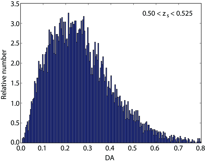
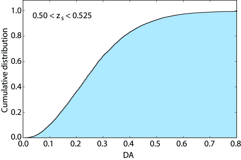
Figure 1: Top panel: The distribution of frequency versus area differential $DA$ for a mock sample with source shell $0.5<z_{s}<0.525$; and Bottom panel: its corresponding cumulative probability distribution.

The $R_{\rm h}=ct$ universe 16 ; 17 ; 52 ; 53 ; 54 is also an FRW cosmology with radiation (photons and neutrinos), matter (baryonic and dark) and dark energy, with radiation and dark energy dominating the early Universe, and matter and dark energy dominating the current era 55 . But while it is similar to $\Lambda$CDM in this regard, it has an additional constraint on the total equation of state, i.e., $\rho+3p=0$, the so-called zero active mass condition, where $\rho$ and $p$ are the total energy density and pressure, respectively. With this additional constraint, the $R_{\rm h}=ct$ universe always expands at a constant rate, which depends on only one parameter—the Hubble constant $H_{0}$. Using the Friedmann equation with zero active mass, we find that

$$H^{R_{\rm h}=ct}(z)=H_{0}(1+z)\;,$$ (14)

and from Equation (12), we therefore find that

$$D_{A}^{R_{\rm h}=ct}(z_{1},z_{2})=\frac{c}{H_{0}}\frac{1}{(1+z_{2})}\ln\left(\frac{1+z_{2}}{1+z_{1}}\right)\;.$$ (15)

5 The Area Minimization Statistic

Now that we are dealing with a comparison between two continuous functions, i.e., $\mathcal{D}_{\rm obs}$ with either $\mathcal{D}^{\rm\Lambda{\rm CDM}}$ or $\mathcal{D}^{R_{\rm h}=ct}$ (each derived from Eq. 5 using Eqs. 13 and 15), we cannot use discrete sampling statistics, such as weighted least squares, for the comparison of different models. The reason is that sampling at random points to obtain the squares of differences between model and reconstructed curve would lose information between these points, whose importance cannot be ascertained prior to the sampling. To overcome this deficiency, we introduce a new statistic, based on a previous application 56 ; 57 , which we call the “Area Minimization Statistic” to estimate each model’s probability of being consistent with the data. Our principal assumption is that the measurement errors are Gaussian, which we use to generate a mock sample of GP reconstructed curves representing the possible variation of $\mathcal{D}$ away from $\mathcal{D}_{\rm obs}$. We do this by employing the Gaussian randomization

$$\mathcal{D}_{i}(z_{l},\langle z_{s}\rangle)=\mathcal{D}_{i,\,{\rm obs}}(z_{l},\langle z_{s}\rangle)+r\sigma_{\mathcal{D}_{i}}\;,$$ (16)

where $\mathcal{D}_{i,\,{\rm obs}}(z_{l},\langle z_{s}\rangle)$ are the actual measurements as a function of $z_{l}$ for each source shell $\langle z_{s}\rangle$. $\sigma_{\mathcal{D}_{i}}$ are the actual observed errors and $r$ is a Gaussian random variable with zero mean and a variance of $1$. Next, these $\mathcal{D}_{i}(z_{l},\langle z_{s}\rangle)$ are used together with the errors $\sigma_{\mathcal{D}_{i}}$ to reconstruct the function $\mathcal{D}_{\rm mock}(z_{l},\langle z_{s}\rangle)$ corresponding to each mock sample, and finally we calculate the weighted absolute area difference between $\mathcal{D}_{\rm mock}(z_{l},\langle z_{s}\rangle)$ and the GP reconstructed function of the actual data according to

$$DA=\int_{z_{\rm min}}^{z_{\rm max}}dz_{l}\bigg{(}\frac{\big{|}\mathcal{D}_{\rm mock}(z_{l},\langle z_{s}\rangle)-\mathcal{D}_{\rm obs}(z_{l},\langle z_{s}\rangle)\big{|}}{\sigma(z_{l})}\bigg{)}\;.$$ (17)

In this expression, $z_{\rm min}$ and $z_{\rm max}$ are the minimum and maximum redshifts, respectively, of the data range. We repeat this procedure $10,000$ times to build a distribution of frequency versus area differential $DA$, and from it construct the cumulative probability distribution. In figure 1 we show these quantities for the illustrative source shell $0.50<z_{s}<0.525$ (the frequency is shown in the top panel, and the cumulative probability distribution is on the bottom). This procedure generates a 1-to-1 mapping between the value of $DA$ and the frequency with which it arises. With the additional assumption that curves with a smaller $DA$ are a better match to $\mathcal{D}_{\rm obs}$, one can then use the cumulative distribution to estimate the probability that the difference between a model’s prediction and the reconstructed curve is merely due to Gaussian randomness. When comparing a model’s prediction to the data, we therefore calculate its $DA$ and use our 1-to-1 mapping to determine the probability that its inconsistency with the data is just due to variance, rather than the model being wrong. These are the probabilities we then compare to determine which model is more likely to be correct. This basic concept is common to many kinds of statistical approaches, though none of the existing ones can be used when comparing two continuous curves, as we have here.

The reconstructed curves for our 5 subsamples are shown in the left-hand panels of figure 2. These correspond to the 5 source redshift shells in Tables 1 to 5. The corresponding cumulative probability distributions are plotted in the right-hand panels, which also locate the $DA$ values for $R_{\rm h}=ct$ (yellow) and $\Lambda$CDM (red). The probabilities associated with these differential areas are summarized in Table 6. Along with the reconstructed functions, the left-hand panels also show the corresponding $1\sigma$ (dark) and $2\sigma$ (light) confidence regions provided by the GP, and the theoretical predictions in $\Lambda$CDM (dashed) and $R_{\rm h}=ct$ (dotted). As we highlighted earlier, the functions $\mathcal{D}_{\rm obs}(z_{l},\langle z_{s}\rangle)$ have been reconstructed without pre-assuming any parametric form, so in principle they represent the actual variation of $\mathcal{D}$ with redshift, regardless of whether or not either of the two models being tested here is the correct cosmology.

The overall impression one gets from the results displayed in figure 2 and summarized in Table 6 is that, for every source redshift shell sampled here, the probability of $R_{\rm h}=ct$ being consistent with the GP reconstructed function $\mathcal{D}_{\rm obs}$ is $\sim 10-30\%$ higher than that for $\Lambda$CDM. Future surveys will greatly grow the sample of sources available for this type of analysis, differentiating between these two models with greater confidence.

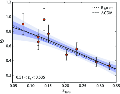
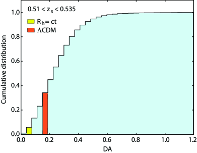
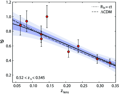
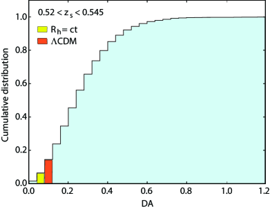
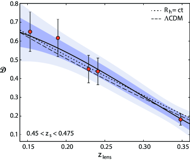
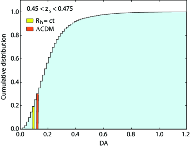
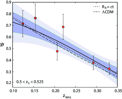
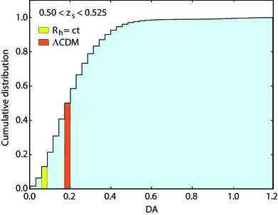
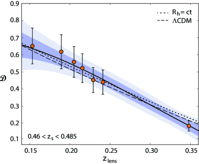
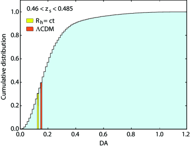
Figure 2: Left Panels (2a, 2c, 2e, 2g, 2i): The solid curve in each plot indicates the reconstructed $\mathcal{D}_{\rm obs}$ function using Gaussian processes, for the source redsfhit ranges $(0.51,0.535)$, $(0.52,0.545)$, $(0.45,0.475)$, $(0.5,0.525)$, and $(0.46,0.485)$. The dotted curve indicates the predicted $\mathcal{D}$ in the $R_{\rm h}=ct$ universe and the dashed curve indicates the corresponding $\mathcal{D}$ in $\Lambda$CDM. In each of these figures, dark blue represents the $1\sigma$ confidence region, and light blue is $2\sigma$. Right Panels (2b, 2d, 2f, 2h, 2j): The corresponding cumulative probability distributions.

Table 6. Model Comparison using Strong Gravitational Lenses with Gaussian Processes

Source Redshift Range	Number of Lenses	$R_{\rm h}=ct$	$\Lambda$CDM	Figures
		Probability	Probability
$0.51-0.535$	9	$94.23\%$	$65.82\%$	2a, 2b
$0.52-0.545$	9	$93.59\%$	$85.48\%$	2c, 2d
$0.46-0.485$	7	$69.43\%$	$60.29\%$	2e, 2f
$0.50-0.525$	6	$86.96\%$	$49.91\%$	2g, 2h
$0.45-0.475$	5	$80.65\%$	$69.68\%$	2i, 2j

6 Conclusions

In this paper, we have introduced the GP reconstruction approach to strong lensing studies, though clearly the available sample is still not large enough for us to make full use of this method. As noted earlier, one of the principal benefits of this technique is that the function (in this case $\mathcal{D}_{\rm obs}$) representing the data may be obtained without the assumption of any parametric form associated with particular models. This allows one to test different models against the actual $\mathcal{D}_{\rm obs}$, rather than against each other’s predictions, neither of which may be a good representation of the measurements. In addition, GP provide $1\sigma$ and $2\sigma$ confidence regions for the reconstructed functions more in line with the population as a whole, rather than individual data points, greatly restricting the ability of ‘incorrect’ models to adequately fit the observations due to otherwise large measurement errors.

This is reflected in the probabilities quoted in Table 6 for the two models we have examined here. Unlike previous model comparisons based on the use of parametric fits to the strong-lensing data, we now find that $R_{\rm h}=ct$ is favoured over $\Lambda$CDM with consistently higher likelihoods in all 5 source redshift shells we have assembled for this work. Though these statistics are still quite limited, it is nonetheless telling that the differentiation between models improves as the number of sources within each shell increases. Also, at least for $R_{\rm h}=ct$, the probability of its predictions matching the GP reconstructed functions generally increases as the size of the lens sample grows. The outcome of this work underscores the importance of using unbiased data and sound statistical methods when comparing different cosmological models. As a counterexample, consider the use of $H(z)$ measurements based on BAO observations instead of cosmic chronometers 28 , constituting an unwitting use of model-dependent measurements to test competing models. Such an approach ignores the significant limitations in all but the three most recent BAO measurements 58 ; 59 for this type of work. Previous applications of the galaxy two-point correlation function to measure the BAO scale were contaminated with redshift distortions associated with internal gravitational effects 59 . To illustrate the significance of these limitations, and the impact of the biased BAO measurements of $H(z)$, note how the model favoured by the data switches from $\Lambda$CDM to $R_{\rm h}=ct$ when only the unbiased measurements are used 61 .

A second counterexample is provided by the merger of disparate sub-samples of Type Ia SNe to improve the statistical analysis. We have already published an in-depth explanation of the perils associated with the blending of data with different systematics for the purpose of model selection 62 , but let us nonetheless consider a brief synopsis here. The Union2.1 catalog 63 ; 64 includes $\approx 580$ SN detections, though each sub-sample has its own systematic and intrinsic uncertainties. The conventional approach minimizes an overall $\chi^{2}$, while each sub-sample is assigned an intrinsic dispersion to ensure that $\chi^{2}_{\rm dof}=1$ 28 ; 29 . Instead, the statistically correct approach would estimate the unknown intrinsic dispersions simultaneously with all other parameters 62 ; 65 . Quite tellingly, the outcome of the model selection is reversed when one switches from the improper statistical approach to the correct one. To emphasize how critical this reversal is in the case of $\Lambda$CDM, one simply needs to compare the outcome of using a merged super-sample with that produced with a large, single homogeneous sample, such as the Supernova Legacy Survey Sample 66 .

Within this context, we highlight the fact that the features of the GP reconstruction approach in the study of strong lenses are promising because, in spite of the fact that the use of these systems to measure cosmological parameters has been with us for over a decade (see, e.g., refs. 4 ; 5 ; 6 ; 67 ), the results of this effort have thus far been less precise than those of other kinds of observations. For the large part, these earlier studies were based on the use of parametric fits to the data, but it is quite evident (e.g., from figures 1 and 2 in ref. 7 ) that the scatter in $\mathcal{D}_{\rm obs}$ about the theoretical curves generally increases significantly as $D_{A}(z_{l},z_{s})\rightarrow D_{A}(0,z_{s})$. That is, measuring $\mathcal{D}$ incurs a progressively greater error as the distance to the gravitational lens becomes a smaller fraction of the distance to the quasar source. This has to do with the fact that $\theta_{\rm E}$ changes less for large values of $z_{s}/z_{l}$ so, for a fixed error in the Einstein angle, the measurement of $\mathcal{D}_{\rm obs}$ becomes less precise. As we have demonstrated in this paper, the analysis of strong lensing systems based on a GP reconstruction of $\mathcal{D}_{\rm obs}$ improves our ability to distinguish between different models, albeit by a modest amount given the current sample.

Upcoming survey projects, such as the Dark Energy Survey (DES; 68 ), the Large Synoptic Survey Telescope (LSST; 69 ), the Joint Dark Energy Mission (JDEM; 70 ), and the Square Kilometer Array (SKA; e.g., ref. 71 ), are expected to greatly grow the size of the lens sample. The ability of GP reconstruction methods to differentiate between models will increase in tandem with this growth. Several sources of uncertainty still remain, however, including the actual mass distribution within the lens. And since such errors appear to be more restricting for lens systems with large values of $z_{s}/z_{l}$, a priority for future work should be the identification of strong lenses with small angular diameter distances between the source and lens relative to the distance between the lens and observer.

- (1) M. Bartelmann & P. Schneider, A&A 345 (1999) 17
- (2) A. Refreiger, ARA&A 41 (2003) 645
- (3) T. Futamase & S. Yoshida, S., PThPh 105 (2001) 887
- (4) T. Treu, L.V.E. Koopmans, A. S. Bolton, S. Burles & L. A. Moustakas, ApJ 640 (2006) 662
- (5) C. Grillo, M. Lombardi & G. Bertin, A&A 477 (2008) 397
- (6) M. Biesiada, A. Piórkowska & B. Malec, B., MNRAS 406 (2010) 1055
- (7) F. Melia, J.-J. Wei & X.-F. Wu, AJ 149 (2015) 2
- (8) S. Cao et al., ApJ 806 (2015) 185
- (9) Y. Shu et al., ApJ 851 (2017) 48
- (10) A. Bolton, S. M. Burles, L.V.E. Koopmans, T. Treu & L. M. Moustakas, ApJ 638 (2006) 703
- (11) L.V.E. Koopmans, T. Treu, A. S. Bolton, S. Burles & L. A. Moustakas, ApJ 649 (2006) 599
- (12) A. S. Bolton, S. M. Burles, L.V.E. Koopmans et al., ApJ 682 (2008) 964
- (13) E. R. Newton, P. J. Marshall & T. Treu, (SLACS Collaboration), ApJ 734 (2011) 104
- (14) A. G. Riess et al., AJ 116 (1998) 1009
- (15) S. Perlmutter et al., Nature 391 (1998) 51
- (16) F. Melia, MNRAS 382 (2007) 1917
- (17) F. Melia & A. Shevchuk, MNRAS 419 (2012) 2579
- (18) F. Melia, MNRAS 464 (2017) 1966
- (19) F. Melia, ApJ 764 (2013) 72
- (20) J.-J. Wei, X. Wu & F. Melia, ApJ 772 (2013) 43
- (21) J.-J. Wei, X.-F. Wu, F. Melia & R. S. Maier, AJ 149 (2015) 102
- (22) F. Melia, J.-J. Wei, R. S. Maier & X. Wu, AJ, submitted (2017)
- (23) F. Melia R. S. Maier, MNRAS 432 (2013) 2669
- (24) P. van Oirschot, J. Kwan & G. F. Lewis, MNRAS 404 (2010) 1633
- (25) M. Bilicki & M. Seikel, MNRAS 425 (2012) 1664
- (26) G. F. Lewis & P. van Oirschot, MNRAS Letters 423 (2012) 26
- (27) G. F. Lewis, MNRAS 432 (2013) 2324
- (28) D. L. Shafer, Phys. Rev. D 91 (2015) 103516
- (29) D. Rubin & B. Hayden B., ApJL 833 (2016) id. L30
- (30) O. Bikwa, F. Melia & A.S.H. Shevchuk, MNRAS 421 (2012) 3356
- (31) F. Melia, JCAP 09 (2012) 029
- (32) F. Melia, Astrop. & Sp. Sc. 356 (2015) 393
- (33) F. Melia, MNRAS 446 (2015) 1191
- (34) K. U. Ratnatunga, R. E. Griffiths & E. J. Ostrander, AJ 117 (1999) 2010
- (35) P. Schneider, J. Ehlers & E. E. Falco, “Gravitational Lenses” (Berlin:Springer) (1992)
- (36) R. Kormann, P. Schneider & M. Bartelmann, A&A 284 (1994) 285
- (37) R. E. White & D. S. Davis, BAAS 28 (1996) 1323
- (38) A. S. Bolton, S. M. Burles, L.V.E. Koopmans, T. Treu & L. M. Moustakas, ApJL 624 (2005) L21
- (39) G. van de Ven, P. G. van Dokkum & M. Franx, MNRAS 344 (2003) 924
- (40) S. Cao, Y. Pan, M. Biesiada, W. Godlowski & Z.-H. Zhu, JCAP 3 (2012) 16
- (41) P. Young, J. E. Gunn, J. Kristian, J. B. Oke & J. A. Westphal, ApJ 241 (1980) 507
- (42) J. Huchra, M. Gorenstein, S. Kent et al., AJ 90 (1985) 691
- (43) J. Lehar, G. I. Langston, A. Silber, C. R. Lawrence & B. F. Burke, AJ 105 (1993) 847
- (44) C. D. Fassnacht, D. S. Womble, G. Neugebauer et al., ApJL 460 (1996) L103
- (45) J. L. Tonry, AJ 115 (1998) 1
- (46) L.V.E. Koopmans & T. Treu, ApJ 568 (2002) 5
- (47) L.V.E. Koopmans & T. Treu, ApJ 583 (2003) 606
- (48) T. Treu & L.V.E. Koopmans, ApJ 611 (2004) 739
- (49) T. Treu & L.V.E. Koopmans, MNRAS 343 (2003) 29
- (50) T. Treu & L.V.E. Koopmans, ApJ 575 (2002) 87
- (51) M. Seikel, C. Clarkson & M. Smith, M., JCAP 06 (2012) 036S
- (52) F. Melia & M. Abdelqader, IJMP-D 18 (2009) 1889
- (53) F. Melia, Frontiers of Physics 11 (2016) 119801
- (54) F. Melia, Fronters of Physics 12 (2017) 129802
- (55) F. Melia & M. Fatuzzo, MNRAS 456 (2016) 3422
- (56) Yennapureddy, M. K. & Melia F, JCAP 11 (2017) 029Y
- (57) F.Melia & Yennapureddy, M. K, JCAP 02 (2018) 034M
- (58) L. Anderson et al., MNRAS 441 (2014) 24
- (59) T. Delubac et al., A&A 574 (2015) A59
- (60) M. López-Corredoira, ApJ 781 (2014) id. 96
- (61) F. Melia & M. López-Corredoira, IJMP-D 26 (2017) 1750055
- (62) J.-J. Wei, X. Wu, F. Melia & R. S. Maier, AJ 149 (2015) 102
- (63) M. R. Kowalski, ApJ 686 (2008) 749
- (64) N. Suzuki et al., ApJ 746 (2012) 85
- (65) A. G. Kim, PASP 123 (2011) 230
- (66) M. Betoule et al., A&A 568 (2014) 22
- (67) M. Biesiada, B. Malec & A. Piórkowska, RAA 11 (2011) 641
- (68) J. Frieman & Dark Energy Survey Collaboration, BAAS 36 (2004) 1462
- (69) A. Tyson & R. Angel, in The New Era of Wide Field Astronomy, ASP Conference Series, Vol. 232. Ed. R. Clowes, A. Adamson & G. Bromage. San Francisco: ASP, p.347 (2001)
- (70) A. Tyson, in ASP Conference Series, Vol. 339, Observing Dark Energy, Ed. S. C. Wolff & T. R. Lauer, p. 95 (2005)
- (71) J. McKean, N. Jackson, S. Vegetti, M. Rybak, S. Serjeant, L.V.E. Koopmans, R. B. Metcalf, C. Fassnacht, P. J. Marshall & M. Pandey-Pommier, in Proceedings of Advancing Astrophysics with the Square Kilometre Array (AASKA14). 9-13 June, 2014. Giardini Naxos, Italy (2015)