Linear-time geometric algorithm for evaluating Bézier curves

Abstract

A new algorithm for computing a point on a polynomial or rational curve in Bézier form is proposed. The method has a geometric interpretation and uses only convex combinations of control points. The new algorithm‘s computational complexity is linear with respect to the number of control points and its memory complexity is $O(1)$. Some remarks on similar methods for surfaces in rectangular and triangular Bézier form are also given.

1 Introduction

Let $b_{k}:D\rightarrow\mathbb{R}$ $(k=0,1,\ldots,N;\,N\in\mathbb{N})$ be real-valued multivariable functions such that

$$b_{k}(\bm{t})\geq 0,\quad\sum_{k=0}^{N}b_{k}(\bm{t})\equiv 1$$ (1.1)

for $\bm{t}\in C\subseteq D$.

Let us define the rational parametric object $\mbox{{S}}_{N}:C\rightarrow\mathbb{E}^{d}$ $(d\in\mathbb{N})$ by

$$\mbox{{S}}_{N}(\bm{t}):=\frac{\displaystyle\sum_{k=0}^{N}\omega_{k}\mbox{{W}}_{k}b_{k}(\bm{t})}{\displaystyle\sum_{k=0}^{N}\omega_{k}b_{k}(\bm{t})}$$ (1.2)

with the weights $\omega_{k}>0$, and control points $\mbox{{W}}_{k}\in\mathbb{E}^{d}$ $(0\leq k\leq N)$. If $\omega_{0}=\omega_{1}=\ldots=\omega_{N}$, then

$$\mbox{{S}}_{N}(\bm{t})=\sum_{k=0}^{N}\mbox{{W}}_{k}b_{k}(\bm{t}).$$

In the sequel, we prove that for a given $\bm{t}\in C$, the point $\mbox{{S}}_{N}(\bm{t})\in\mathbb{E}^{d}$ can be computed by Algorithm 1.1.

Algorithm 1.1 Computation of $\mbox{{S}}_{N}(\bm{t})$

1:procedure GenAlg($N,\bm{t},\omega,\mbox{{W}}$)

2:     $h_{0}\leftarrow 1$

3:     $\mbox{{Q}}_{0}\leftarrow\mbox{{W}}_{0}$

4:     for $k\leftarrow 1,N$ do

5:         $h_{k}\leftarrow\left(1+\frac{\displaystyle\omega_{k-1}b_{k-1}(\bm{t})}{\displaystyle h_{k-1}\omega_{k}b_{k}(\bm{t})}\right)^{-1}$

6:

7:         $\mbox{{Q}}_{k}\leftarrow(1-h_{k})\mbox{{Q}}_{k-1}+h_{k}\mbox{{W}}_{k}$

8:     end for

9:     return $\mbox{{Q}}_{N}$

10:end procedure

Remark 1.1.

Let us fix $\bm{t}\in C$. Suppose that there exists $1\leq k\leq N$ such that $b_{k}(\bm{t})=0$. Then one has the division by $0$ in the line 5 of Algorithm 1.1. Such special cases should be considered separately. Observe that it is always possible because at least for one $0\leq j\leq N$ we have $b_{j}(\bm{t})>0$ (cf. (1.1)).

Theorem 1.2.

The quantities $h_{k}$ and $\mbox{{Q}}_{k}$ $(0\leq k\leq N)$ computed by Algorithm 1.1 have the following properties:

1. $h_{k}\in[0,1]$,

2. $\mbox{{Q}}_{k}\in\mathbb{E}^{d}$,

3. $\mbox{{Q}}_{k}\in C_{k}\equiv\mbox{conv}\{\mbox{{W}}_{0},\mbox{{W}}_{1},\ldots,\mbox{{W}}_{k}\}$ (i.e., $\mbox{conv}\{\mbox{{Q}}_{0},\mbox{{Q}}_{1},\ldots,\mbox{{Q}}_{k}\}\subseteq C_{k}$).

Moreover, $\mbox{{S}}_{N}(\bm{t})=\mbox{{Q}}_{N}$.

Proof.

Let us define

$$h_{k}:=\frac{\displaystyle\omega_{k}b_{k}(\bm{t})}{\displaystyle\sum_{j=0}^{k}\omega_{j}b_{j}(\bm{t})},\quad\mbox{{Q}}_{k}:=\frac{\displaystyle\sum_{j=0}^{k}\omega_{j}\mbox{{W}}_{j}b_{j}(\bm{t})}{\displaystyle\sum_{j=0}^{k}\omega_{j}b_{j}(\bm{t})}$$

$(k=0,1,\ldots,N)$.

It is clear that $h_{k}\in[0,1]$, $\mbox{{Q}}_{k}\in{\mathbb{E}^{d}}$ for $0\leq k\leq N$, $h_{0}=1$, $\mbox{{W}}_{0}=\mbox{{Q}}_{0}$, and $\mbox{{S}}_{N}(\bm{t})=\mbox{{Q}}_{N}$. Certainly,

$$\mbox{{Q}}_{k}\in\mbox{conv}\{\mbox{{W}}_{0},\mbox{{W}}_{1},\ldots,\mbox{{W}}_{k}\}\quad(0\leq k\leq N).$$

To end the proof, it is enough to check that:

$$\left\{\begin{array}[]{l}(1-h_{k})\mbox{{Q}}_{k-1}+h_{k}\mbox{{W}}_{k}=\mbox{{Q}}_{k},\\[4.30554pt] \omega_{k}b_{k}(\bm{t})h_{k}^{-1}=\omega_{k-1}b_{k-1}(\bm{t})h_{k-1}^{-1}+\omega_{k}b_{k}(\bm{t})\end{array}\right.$$

for $1\leq k\leq N$ (cf. lines 5, 6 in Algorithm 1.1). ∎

Let us notice that Algorithm 1.1 has a geometric interpretation, uses only convex combinations of control points of $\mbox{{S}}_{N}$ and has linear complexity with respect to $N$ — under the assumption that all quotients of two consecutive basis functions can be computed in the total time $O(N)$.

Remark 1.3.

It may be worth mentioning that

$$1-h_{k}=\frac{h_{k}}{h_{k-1}}\frac{\omega_{k-1}b_{k-1}(\bm{t})}{\omega_{k}b_{k}(\bm{t})}$$ (1.3)

for $1\leq k\leq N$. Using this simple relation, one can propose a subtraction-free version of Algorithm 1.1. Such formulation can be important for numerical reasons (cf. the problem of cancellation of digits; see, e.g., [2, §2.3.4]).

We use relation (1.3) in the proof of the following theorem which shows an important property of Algorithm 1.1.

Theorem 1.4.

Let us fix $\bm{t},\bm{u}\in C$. Assume that the numbers $h_{k}$ $(1\leq k\leq N)$ computed by Algorithm 1.1 are non-zero. Suppose that

$$\frac{b_{k}(\bm{t})}{b_{k+1}(\bm{t})}\leq\frac{b_{k}(\bm{u})}{b_{k+1}(\bm{u})}\quad(0\leq k\leq N-1).$$

Then the point $\mbox{{S}}_{N}(\bm{u})\in{\mathbb{E}^{d}}$ is in the convex hull of the points $\mbox{{Q}}_{0},\mbox{{Q}}_{1},\ldots,\mbox{{Q}}_{N}$ computed by Algorithm 1.1.

Proof.

Let the numbers $h_{k}$ and the points $\mbox{{Q}}_{k}$ $(0\leq k\leq N)$ be computed by Algorithm  1.1 for a fixed $\bm{t}\in C$.

Using relation (1.3) and the assumption that $h_{k}\neq 0$ $(1\leq k\leq N)$, observe that

$$\mbox{{W}}_{k}=h_{k}^{-1}\mbox{{Q}}_{k}-h_{k-1}^{-1}\frac{\omega_{k-1}b_{k-1}(\bm{t})}{\omega_{k}b_{k}(\bm{t})}\mbox{{Q}}_{k-1}$$

for $1\leq k\leq N$. Thus, after simple algebra, we obtain

$$\mbox{{S}}_{N}(\bm{u})=D_{N}(\bm{u})^{-1}\Bigg{(}\frac{\omega_{N}}{h_{N}}b_{N}(\bm{u})\cdot\mbox{{Q}}_{N}$$

$$+\sum_{k=0}^{N-1}\frac{\omega_{k}}{h_{k}}b_{k}(\bm{u})\left(1-\frac{b_{k}(\bm{t})b_{k+1}(\bm{u})}{b_{k+1}(\bm{t})b_{k}(\bm{u})}\right)\cdot\mbox{{Q}}_{k}\Bigg{)},$$

where $D_{N}(\bm{u}):=\sum_{k=0}^{N}\omega_{k}b_{k}(\bm{u})>0$.

Now, from our assumptions, it easily follows that the point $\mbox{{S}}_{N}(\bm{u})$ belongs to the set $\mbox{conv}\{\mbox{{Q}}_{0},\mbox{{Q}}_{1},\ldots,\mbox{{Q}}_{N}\}$, because the $h_{k}$ $(0\leq k\leq N)$ are positive (cf. Theorem 1.2). ∎

The main aim of this article is to use the presented results to propose a new method for evaluating a polynomial or rational Bézier curve, which has a geometric interpretation, linear complexity with respect to the number of control points, good numerical properties and computes only convex combinations of points from ${\mathbb{E}^{d}}$. See Section 2.

A similar approach can also be used for the evaluation of polynomial and rational tensorproduct, as well as triangular, Bézier surfaces. Some remarks on this issue are given, without technical details and rigorous algorithms, in Section 3.

2 New algorithm for evaluating Bézier curves

Let there be given points $\mbox{{W}}_{0},\mbox{{W}}_{1},\ldots,\mbox{{W}}_{n}\in\mathbb{E}^{d}$ $(n,d\in\mathbb{N})$. Let us consider the (polynomial) Bézier curve of the form

$$\mbox{{P}}_{n}(t):=\sum_{k=0}^{n}\mbox{{W}}_{k}B^{n}_{k}(t)\quad(t\in[0,1]),$$ (2.1)

where $B^{n}_{k}$ is the $k$th Bernstein polynomial of degree $n$,

$$B^{n}_{k}(t):=\binom{n}{k}t^{k}(1-t)^{n-k}\quad(0\leq k\leq n).$$ (2.2)

For a given $t\in[0,1]$, the point $\mbox{{P}}_{n}(t)\in\mathbb{E}^{d}$ can be computed by famous the de Casteljau algorithm (see, e.g., [3, §4.2] and Appendix), which has good numerical properties, a simple geometric interpretation and computes only convex combinations of control points $\mbox{{W}}_{k}$ $(0\leq k\leq n)$. However, the computational complexity of this method is $O(dn^{2})$, which makes it quite expensive.

Probably, the fastest way to compute the coordinates of the point $\mbox{{P}}_{n}(t)\in\mathbb{E}^{d}$ is to use the algorithm proposed in [5] for evaluating a polynomial $p$ given in the form

$$p(t):=\sum_{k=0}^{n}p_{k}t^{k}(1-t)^{n-k}\quad(p_{k}\in\mathbb{R})$$

$d$ times (once for each dimension). This method has $O(dn)$ computational complexity and $O(1)$ memory complexity. It uses the concept of Horner‘s rule (see, e.g., [2, Eq. (1.2.2)]).

Note that some other methods for evaluating a Bézier curve are also known. See, e.g., [1] or [4], where the case of Bézier surfaces was also studied (cf. Section 3), and papers cited therein.

Let $\mbox{{R}}_{n}$ be a rational Bézier curve in $\mathbb{E}^{d}$,

$$\mbox{{R}}_{n}(t):=\frac{\displaystyle\sum_{k=0}^{n}\omega_{k}\mbox{{W}}_{k}B^{n}_{k}(t)}{\displaystyle\sum_{k=0}^{n}\omega_{k}B^{n}_{k}(t)}\quad(t\in[0,1])$$ (2.3)

with the weights $\omega_{0},\omega_{1},\ldots,\omega_{n}\in\mathbb{R}_{+}$. To compute the point $\mbox{{R}}_{n}(t)\in\mathbb{E}^{d}$ for a given $t\in[0,1]$, one can use the rational de Casteljau algorithm (see, e.g., [3, §13.2] and Appendix), which also has $O(dn^{2})$ computational complexity, good numerical properties, a geometric interpretation and computes only convex combinations of the control points $\mbox{{W}}_{k}$ $(0\leq k\leq n)$, or use the idea from [5], which leads to linear-time method at the cost of losing some geometric properties.

The main purpose of this section is to propose a new efficient method for computing a point on a Bézier curve and on a rational Bézier curve. The given algorithm has:

1. a geometric interpretation,

2. quite good numerical properties, i.e., they are safe for floating-point computations,

3. linear computational complexity, i.e., $O(dn)$, and $O(1)$ memory complexity,

and computes only

1. convex combinations of control points.

As we show later, the new method combines the advantages of de Casteljau algorithms and the low complexity of methods based on [5].

2.1 New method

Let $\mbox{{R}}_{n}$ be the rational Bézier curve (2.3). Let us fix: a parameter $t\in[0,1]$, a natural number $n$, weights $\omega_{0},\omega_{1},\ldots,\omega_{n}>0$ and control points $\mbox{{W}}_{0},\mbox{{W}}_{1},\ldots,\mbox{{W}}_{n}\in\mathbb{E}^{d}$ $(d\in\mathbb{N})$.

Let the quantities $h_{k}$ and $\mbox{{Q}}_{k}$ $(0\leq k\leq n)$ be computed recursively by formulas

$$\left\{\begin{array}[]{l}h_{0}:=1,\quad\mbox{{Q}}_{0}:=\mbox{{W}}_{0},\\[4.30554pt] h_{k}:=\frac{\displaystyle\omega_{k}h_{k-1}t(n-k+1)}{\displaystyle\omega_{k-1}k(1-t)+\omega_{k}h_{k-1}t(n-k+1)},\\[10.76385pt] \mbox{{Q}}_{k}:=(1-h_{k})\mbox{{Q}}_{k-1}+h_{k}\mbox{{W}}_{k}\end{array}\right.$$ (2.4)

for $k=1,2,\ldots,n$.

Theorem 2.1.

For all $k=0,1,\ldots,n$, the quantities $h_{k}$ and $\mbox{{Q}}_{k}$ satisfy:

1. $h_{k}\in[0,1]$,

2. $\mbox{{Q}}_{k}\in\mathbb{E}^{d}$,

3. $\mbox{{Q}}_{k}\in C_{k}\equiv\mbox{conv}\{\mbox{{W}}_{0},\mbox{{W}}_{1},\ldots,\mbox{{W}}_{k}\}$ (i.e., $\mbox{conv}\{\mbox{{Q}}_{0},\mbox{{Q}}_{1},\ldots,\mbox{{Q}}_{k}\}\subseteq C_{k}$).

Moreover, we have $\mbox{{R}}_{n}(t)=\mbox{{Q}}_{n}$.

Proof.

The proof goes in a similar way to that of Theorem 1.2, where $N:=n$, $b_{k}(\bm{t}):=B^{n}_{k}(t)$.

Note that this method is robust — special cases $t=0$ and $t=1$ do not cause division by zero (cf. Remark 1.1) and yield $\mbox{{W}}_{0}$ and $\mbox{{W}}_{n}$, respectively. ∎

In each step of the new method, the point $\mbox{{Q}}_{k}$, which is a convex combination of points $\mbox{{Q}}_{k-1}$ and $\mbox{{W}}_{k}$, is computed. The last point $\mbox{{Q}}_{n}$ is equal to the point $\mbox{{R}}_{n}(t)$. Thus, we obtain the new linear-time geometric algorithm for computing a point on a rational Bézier curve which computes only convex combinations of control points. For efficient implementations, see Section 2.2.

Note that if all weights $\omega_{k}$ are equal then $\mbox{{Q}}_{n}=\mbox{{P}}_{n}(t)$ (cf. (2.1)) — the new method can also be used to evaluate a polynomial Bézier curve.

Figure 2.1 illustrates the new method in case of a planar polynomial Bézier curve of degree $n=5$.

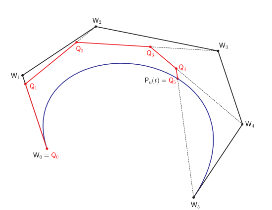
Figure 2.1: Computation of a point on a planar polynomial Bézier curve of degree $n=5$ using the new method.

Using Theorem 1.4, one can prove the following result which tells even more about geometric properties of the new method.

Theorem 2.2.

Let the numbers $h_{k}$ and the points $\mbox{{Q}}_{k}$ $(0\leq k\leq n)$ be computed by (2.4) for a given $0\leq t\leq 1$. The point $\mbox{{R}}_{n}(u)$, where $u\in[0,1]$, is in the convex hull of the points $\mbox{{Q}}_{0},\mbox{{Q}}_{1},\ldots,\mbox{{Q}}_{n}$ if and only if $u\leq t$. It means that

$$\mbox{{R}}_{n}([0,u])\subset\mbox{conv}\{\mbox{{Q}}_{0},\mbox{{Q}}_{1},\ldots,\mbox{{Q}}_{n}\}\quad(u\leq t).$$

Let us notice that the proposed method can also be used for the subdivision of Bézier curve (cf., e.g., [3, §5.4]). For example, let us fix $u\in(0,1)$, it is well-known that the points

$$\mbox{{V}}_{k}:=\sum_{j=0}^{k}B^{k}_{j}(u)\mbox{{W}}_{j}\quad(0\leq k\leq n)$$

are the control points of the polynomial Bézier curve $\mbox{{P}}_{n}^{L}$ being the left part of the Bézier curve (2.1) with $t\in[0,u]$. One can check that

$$\mbox{{V}}_{k}=\sum_{j=0}^{k}h_{j}^{-1}\frac{n-k}{n-j}B^{k}_{j}(u)\mbox{{Q}}_{j}\quad(0\leq k\leq n-1),$$

$\mbox{{V}}_{n}=\mbox{{Q}}_{n}$, where the numbers $h_{j}$ and the points $\mbox{{Q}}_{j}$ $(0\leq j\leq n)$ are computed using (2.4) with $t:=u$, $\omega_{0}=\omega_{1}=\ldots=\omega_{n}:=1$.

2.2 Implementation and cost

Let us give efficient and numerically safe implementations of the new method which have $O(dn)$ computational complexity and $O(1)$ memory complexity.

Algorithm 2.1 First implementation

1:procedure NewRatBEval1($n,t,\omega,\mbox{{W}}$)

2:     $h\leftarrow 1$

3:     $u\leftarrow 1-t$

4:     $n_{1}\leftarrow n+1$

5:     $\mbox{{Q}}\leftarrow\mbox{{W}}_{0}$

6:     for $k\leftarrow 1,n$ do

7:         $h\leftarrow h\cdot t\cdot(n_{1}-k)\cdot\omega_{k}$

8:         $h\leftarrow h/(k\cdot u\cdot\omega_{k-1}+h)$

9:         $h_{1}\leftarrow 1-h$

10:         $\mbox{{Q}}\leftarrow h_{1}\cdot\mbox{{Q}}+h\cdot\mbox{{W}}_{k}$

11:     end for

12:     return Q

13:end procedure

The implementation provided in Algorithm 2.1 requires $(3d+8)n+1$ floating-point arithmetic operations (flops) to compute a point on a rational Bézier curve of degree $n$ in $\mathbb{E}^{d}$.

Algorithm 2.2 Second implementation

1:procedure NewRatBEval2($n,t,\omega,\mbox{{W}}$)

2:     $h\leftarrow 1$

3:     $u\leftarrow 1-t$

4:     $n_{1}\leftarrow n+1$

5:     $\mbox{{Q}}\leftarrow\mbox{{W}}_{0}$

6:     if $t\leq 0.5$ then

7:         $u\leftarrow t/u$

8:         for $k\leftarrow 1,n$ do

9:              $h\leftarrow h\cdot u\cdot(n_{1}-k)\cdot\omega_{k}$

10:              $h\leftarrow h/(k\cdot\omega_{k-1}+h)$

11:              $h_{1}\leftarrow 1-h$

12:              $\mbox{{Q}}\leftarrow h_{1}\cdot\mbox{{Q}}+h\cdot\mbox{{W}}_{k}$

13:         end for

14:     else

15:         $u\leftarrow u/t$

16:         for $k\leftarrow 1,n$ do

17:              $h\leftarrow h\cdot(n_{1}-k)\cdot\omega_{k}$

18:              $h\leftarrow h/(k\cdot u\cdot\omega_{k-1}+h)$

19:              $h_{1}\leftarrow 1-h$

20:              $\mbox{{Q}}\leftarrow h_{1}\cdot\mbox{{Q}}+h\cdot\mbox{{W}}_{k}$

21:         end for

22:     end if

23:     return Q

24:end procedure

Algorithm 2.2 decreases the number of flops to $(3d+7)n+2$. However, for numerical reasons (cf. lines 7 and 15 in Algorithm 2.2), it is necessary to use a conditional statement. More precisely, one has to check whether $t\in[0,0.5]$ or $t\in(0.5,1]$, which can be easily done (it is enough to check an exponent of a floating-point number $t$).

Note that in the case of polynomial Bézier curves (2.1), one only needs to set $\omega_{k}:=1$ $(0\leq k\leq n)$ in the given algorithms, thus simplifying used formulas. Then the number of flops is equal to $(3d+6)n+1$ in Algorithm 2.1 and $(3d+5)n+2$ in Algorithm 2.2.

		new method (cf. Alg. 2.2)	de Casteljau (cf. Appendix)
Bézier curve	in total	$(3d+5)n+2$	$\displaystyle\frac{3dn(n+1)}{2}+1$
	add/sub	$(d+2)n+1$	$\displaystyle\frac{dn(n+1)}{2}+1$
	mult	$2(d+1)n$	$dn(n+1)$
	div	$n+1$	$0$
rational Bézier curve	in total	$(3d+7)n+2$	$\displaystyle\frac{(3d+5)n(n+1)}{2}+1$
	add/sub	$(d+2)n+1$	$\displaystyle\frac{(d+2)n(n+1)}{2}+1$
	mult	$2(d+2)n$	$(d+1)n(n+1)$
	div	$n+1$	$\displaystyle\frac{n(n+1)}{2}$

Table 2.1: Numbers of flops.

The numbers of flops for the new algorithms, as well as for de Casteljau algorithms (see Appendix), which also have a geometric interpretation and compute only convex combinations of control points, are given in Table 2.1.

Example 2.3.

Table 2.2 shows the comparison between the running times of de Casteljau algorithm and Algorithm 2.2 both for Bézier curves and rational Bézier curves (in the case of Bézier curves, Algorithm 2.2 has been simplified), for $d\in\{2,3\}$. The results have been obtained on a computer with Intel Core i5-2540M CPU at 2.60GHz processor and 4GB RAM, using GNU C Compiler 7.4.0 (single precision).

More precisely, we made the following numerical experiments. For a fixed $n$, $10000$ curves of degree $n$ are generated. Their control points $\mbox{{W}}_{k}\in[-1,1]^{d}$ and—in the rational case—weights $\omega_{k}\in[0.01,1]$ $(0\leq k\leq n)$ have been generated using the rand() C function. Each curve is then evaluated at 501 points $t_{i}:=i/500$ $(0\leq i\leq 500)$. Each algorithm is tested using the same curves. Table 2.2 shows the total running time of all $501\times 10000$ evaluations.

		Bézier curve		rational Bézier curve
$n$	$d$	new method (cf. Alg. 2.2)	de Casteljau (cf. Appendix)	new method (cf. Alg. 2.2)	de Casteljau (cf. Appendix)
1	2	2.654	2.603	2.672	2.685
	3	2.660	2.626	2.675	2.713
2	2	2.760	2.694	2.773	2.846
	3	2.751	2.753	2.784	2.938
3	2	2.848	2.854	2.872	3.070
	3	2.842	2.930	2.889	3.316
4	2	2.954	3.028	2.989	3.380
	3	2.927	3.120	2.997	3.853
5	2	3.017	3.238	3.094	3.868
	3	3.015	3.334	3.111	4.279
6	2	3.113	3.551	3.203	4.201
	3	3.064	3.566	3.215	4.768
10	2	3.468	4.447	3.593	6.549
	3	3.466	4.995	3.599	7.634
15	2	3.830	6.194	4.057	10.979
	3	3.878	7.495	4.070	12.977
20	2	4.241	8.461	4.527	17.261
	3	4.284	10.910	4.543	20.482

Table 2.2: Running times comparison (in seconds) for Example 2.3. The source code in C which was used to perform the tests is available at http://www.ii.uni.wroc.pl/~pwo/programs/new-Bezier-eval-main.c.

Observe that in the case of Bézier curves, the quantities $h$, which are computed in the new algorithms, do not depend on the control points. One can use this fact in the fast evaluation of $M$ Bézier curves of the same degree $n$ for the same value of the parameter $t$. Such a method requires $(3dM+5)n+2$ flops while the direct use of the de Casteljau algorithm means that all computations have to be repeated $M$ times, i.e., the number of flops is equal to $3Mdn(n+1)/2+1$.

Remark 2.4.

In rather rare cases $(h_{k}\approx 1)$, the problem of cancellation of digits ([2, §2.3.4]) can occur while $1-h_{k}$ is computed (cf. $h_{1}$ in Algorithms 2.1, 2.2). One can avoid this problem using the relation

$$1-h_{k}=\frac{h_{k}}{h_{k-1}}\frac{\omega_{k-1}k(1-t)}{\omega_{k}t(n-k+1)}\quad(1\leq k\leq n),$$

if computations with high accuracy are necessary.

3 Remarks on evaluation of Bézier surfaces

The method of evaluation described in Section 1 can also be applied to the rational rectangular and triangular Bézier surfaces.

Let $\mbox{{S}}_{mn}:[0,1]^{2}\rightarrow\mathbb{E}^{d}$ $(m,n,d\in\mathbb{N})$ be a rational rectangular Bézier surface with the control points $\mbox{{W}}_{ij}\in\mathbb{E}^{d}$ and weights $\omega_{ij}>0$ $(0\leq i\leq m,\ 0\leq j\leq n)$,

$$\mbox{{S}}_{mn}(s,t):=\frac{\displaystyle\sum_{i=0}^{m}\sum_{j=0}^{n}\omega_{ij}\mbox{{W}}_{ij}B^{m}_{i}(s)B^{n}_{j}(t)}{\displaystyle\sum_{i=0}^{m}\sum_{j=0}^{n}\omega_{ij}B^{m}_{i}(s)B^{n}_{j}(t)}.$$

Define $T:=\{(s,t):s,t\geq 0,\,1-s-t\geq 0\}$. Let there be given the control points $\mbox{{V}}_{ij}\in\mathbb{E}^{d}$ and positive weights $v_{ij}$ $(0\leq i+j\leq n)$. Let $B^{n}_{ij}$ denotes the triangular Bernstein polynomials,

$$B^{n}_{ij}(s,t):=\frac{n!}{i!j!(n-i-j)!}s^{i}t^{j}(1-s-t)^{n-i-j},$$

where $0\leq i+j\leq n$. Let us consider a rational triangular Bézier surface $\mbox{{T}}_{n}:T\rightarrow\mathbb{E}^{d}$ $(n,d\in\mathbb{N})$ of the form

$$\mbox{{T}}_{n}(s,t):=\frac{\displaystyle\sum_{i=0}^{n}\sum_{j=0}^{n-i}v_{ij}\mbox{{V}}_{ij}B^{n}_{ij}(s,t)}{\displaystyle\sum_{i=0}^{n}\sum_{j=0}^{n-i}v_{ij}B^{n}_{ij}(s,t)}.$$

Both surface types are, in fact, rational parametric objects (cf. (1.2)). Thus, one can apply Algorithm 1.1 to propose the methods which have geometric interpretations, compute only convex combinations of points and allow to evaluate Bézier surfaces in linear time with respect to the number of control points, i.e., $O(nm)$ in the rectangular case and $O(n^{2})$ in the triangular case. To do so, it is necessary to rearrange the sets of control points, corresponding weights and basis functions (cf. (1.1)) into one-dimensional sequences — but since the method is agnostic of the ordering, the chosen ordering is only a matter of preference. Taking into account that the computations can be performed in many ways, we do not present rigorous algorithms and we pass some technical details.

In this section, to present a concise formulation of the methods, we choose the row-by-row order. For the reader‘s convenience, the analogues of quantities $h_{k}$ and points $\mbox{{Q}}_{k}$ from Algorithm 1.1 have two indices instead, to correspond with the surfaces‘ structure.

3.1 Rational rectangular Bézier surfaces

Let $\mbox{{S}}_{mn}$ $(m,n\in\mathbb{N})$ be a rational rectangular Bézier surface with the weights $\omega_{ij}$ and control points $\mbox{{W}}_{ij}$ $(0\leq i\leq m,\,0\leq j\leq n)$.

In this case, one can interpret the set of control points as a rectangular grid having $m+1$ rows with $n+1$ points in each row. We set the sequence of control points so that:

• the sequence begins with $\mbox{{W}}_{00}$,

• $\mbox{{W}}_{i,j-1}$ is followed by $\mbox{{W}}_{ij}$ $(0\leq i\leq m,\,1\leq j\leq n)$,

• $\mbox{{W}}_{i-1,n}$ is followed by $\mbox{{W}}_{i0}$ $(1\leq i\leq m)$.

In a similar way, we set the sequences of weights $\omega_{ij}$ and basis functions $B^{m}_{i}(s)B^{n}_{j}(t)$ $(0\leq i\leq m,\,0\leq j\leq n)$.

It is well-known that if $(s,t)$ belongs to the boundary of the square $[0,1]^{2}$ then the point $\mbox{{S}}_{mn}(s,t)$ lies on the boundary rational Bézier curve with boundary control points and weights. Thus, the method described in Section 2.1 can be used in this case.

Let us fix $(s,t)\in(0,1)^{2}$. Now, based on Algorithm 1.1, we define the sequences of quantities $h_{ij}$ and points $\mbox{{Q}}_{ij}\in\mathbb{E}^{d}$ $(0\leq i\leq m,\,0\leq j\leq n)$—determined in the order described above—in the following recurrent way:

$$h_{ij}:=\left\{\begin{array}[]{l}1\quad(i=j=0),\\[6.45831pt] \left(1+\frac{\displaystyle i\omega_{i-1,n}(1-s)t^{n}}{\displaystyle m_{i}\omega_{i0}h_{i-1,n}s(1-t)^{n}}\right)^{-1}\\[8.61108pt] \hfill(i\neq 0,\,j=0),\\[5.38193pt] \left(1+\frac{\displaystyle j\omega_{i,j-1}(1-t)}{\displaystyle n_{j}\omega_{ij}h_{i,j-1}t}\right)^{-1}\\[8.61108pt] \hfill(\mbox{otherwise}),\end{array}\right.$$

$$\mbox{{Q}}_{ij}:=\left\{\begin{array}[]{l}\mbox{{W}}_{00}\quad(i=j=0),\\[3.22916pt] (1-h_{i0})\mbox{{Q}}_{i-1,n}+h_{i0}\mbox{{W}}_{i0}\\[3.22916pt] \hfill(i\neq 0,\,j=0),\\[3.22916pt] (1-h_{ij})\mbox{{Q}}_{i,j-1}+h_{ij}\mbox{{W}}_{ij}\\[3.22916pt] \hfill(\mbox{otherwise}),\end{array}\right.$$

where $0\leq i\leq m,\,0\leq j\leq n$, and $m_{i}:=m-i+1$, $n_{j}:=n-j+1$.

Theorem 1.2 implies that $\mbox{{S}}_{mn}(s,t)=\mbox{{Q}}_{mn}$.

3.2 Rational triangular Bézier surfaces

Suppose $\mbox{{T}}_{n}$ $(n\in\mathbb{N})$ is a rational triangular Bézier surface associated with the weights $v_{ij}$ and control points $\mbox{{V}}_{ij}$ $(0\leq i+j\leq n)$.

The method described below is analogous to the one for rectangular Bézier surfaces. The main difference is that, in this case, the set of the control points can be seen as a triangular grid, i.e., the number of control points in each row depends on the row number. Namely, there are $n-i+1$ points in the $i$th row $(0\leq i\leq n)$ of this triangular grid. We choose the following ordering of control points:

• the sequence begins with $\mbox{{V}}_{00}$,

• $\mbox{{V}}_{i,j-1}$ is followed by $\mbox{{V}}_{ij}$ $(0\leq i\leq n-1,\,1\leq j\leq n-i$),

• $\mbox{{V}}_{i-1,n-i+1}$ is followed by $\mbox{{V}}_{i0}$ $(1\leq i\leq n)$.

We set the sequences of weights $v_{ij}$ and basis functions $B^{n}_{ij}(s,t)$ $(0\leq i+j\leq n)$ in the same way.

Assume $(s,t)$ is on the boundary of the triangle $T$. Then the point $\mbox{{T}}_{n}(s,t)$ lies on the boundary rational Bézier curve having known control points and weights and, again, one can compute this point using the method presented in Section 2.1.

Let us fix a point $(s,t)$ inside the triangle $T$. Similarly, based on Algorithm 1.1, we introduce the sequences of quantities $g_{ij}$ and points $\mbox{{U}}_{ij}\in\mathbb{E}^{d}$ $(0\leq i+j\leq n)$, which are computed in the order described above, by the following recurrent formulas:

$$g_{ij}:=\left\{\begin{array}[]{l}1\quad(i=j=0),\\[6.45831pt] \left(1+\frac{\displaystyle iv_{i-1,n-i+1}t^{n-i+1}}{\displaystyle n_{i}v_{i0}g_{i-1,n-i+1}sr^{n-i}}\right)^{-1}\\[8.61108pt] \hfill(i\neq 0,\,j=0),\\[5.38193pt] \left(1+\frac{\displaystyle jv_{i,j-1}r}{\displaystyle n_{i+j}v_{ij}g_{i,j-1}t}\right)^{-1}\\[8.61108pt] \hfill(\mbox{otherwise}),\end{array}\right.\hfill$$

$$\mbox{{U}}_{ij}:=\left\{\begin{array}[]{l}\mbox{{V}}_{00}\quad(i=j=0),\\[3.22916pt] (1-g_{i0})\mbox{{U}}_{i-1,n-i+1}+g_{i0}\mbox{{V}}_{i0}\\[3.22916pt] \hfill(i\neq 0,\,j=0),\\[3.22916pt] (1-g_{ij})\mbox{{U}}_{i,j-1}+g_{ij}\mbox{{V}}_{ij}\\[3.22916pt] \hfill(\mbox{otherwise}),\end{array}\right.\hfill$$

where $0\leq i\leq n,\,0\leq j\leq n-i$, and $r:=1-s-t$, $n_{l}:=n-l+1$.

Then $\mbox{{T}}_{n}(s,t)=\mbox{{U}}_{n0}$, which follows from Theorem 1.2.

Appendix. Implementations of de Casteljau algorithms for Bézier curves

For the reader‘s convenience, let us also present efficient implementations of de Casteljau algorithms which have $O(n)$ memory complexity. See Algorithms A.1 and A.2 (cf., e.g., [3]). The numbers of flops for these methods are given in Table 2.1.

Algorithm A.1 De Casteljau algorithm

1:procedure BEval($n,t,\mbox{{W}}$)

2:     $t_{1}\leftarrow 1-t$

3:     for $i\leftarrow 0,n$ do

4:         $\mbox{{Q}}_{i}\leftarrow\mbox{{W}}_{i}$

5:     end for

6:     for $k\leftarrow 1,n$ do

7:         for $i\leftarrow 0,n-k$ do

8:              $\mbox{{Q}}_{i}\leftarrow t_{1}\cdot\mbox{{Q}}_{i}+t\cdot\mbox{{Q}}_{i+1}$

9:         end for

10:     end for

11:     return $\mbox{{Q}}_{0}$

12:end procedure

Algorithm A.2 Rational de Casteljau algorithm

1:procedure RatBEval($n,t,\omega,\mbox{{W}}$)

2:     $t_{1}\leftarrow 1-t$

3:     for $i\leftarrow 0,n$ do

4:         $w_{i}\leftarrow\omega_{i}$

5:         $\mbox{{Q}}_{i}\leftarrow\mbox{{W}}_{i}$

6:     end for

7:     for $k\leftarrow 1,n$ do

8:         for $i\leftarrow 0,n-k$ do

9:              $u\leftarrow t_{1}\cdot w_{i}$

10:              $v\leftarrow t\cdot w_{i+1}$

11:              $w_{i}\leftarrow u+v$

12:              $u\leftarrow u/w_{i}$

13:              $v\leftarrow 1-u$

14:              $\mbox{{Q}}_{i}\leftarrow u\cdot\mbox{{Q}}_{i}+v\cdot\mbox{{Q}}_{i+1}$

15:         end for

16:     end for

17:     return $\mbox{{Q}}_{0}$

18:end procedure

References

• [1] L. Bezerra, Efficient computation of Bézier curves from their Bernstein-Fourier representation, Applied Mathematics and Computation 220 (2013) 235–238.
• [2] G. Dahlquist, Å. Björck, Numerical methods in scientific computing. Vol. I, SIAM, Philadelphia, 2008.
• [3] G. Farin, Curves and surfaces for computer-aided geometric design. A practical guide, 5th ed., Academic Press, Boston, 2002.
• [4] J. Peters, Evaluation and approximate evaluation of the multivariate Bernstein-Bézier form on a regularly partitioned simplex, ACM Transactions on Mathematical Software (TOMS) 20 (4) (1994) 460–480.
• [5] L. Schumaker, W. Volk, Efficient evaluation of multivariate polynomials, Computer Aided Geometric Design 3 (1986) 149–154.