Electromagnetic multipole moments of the $P_{c}^{+}(4380)$ pentaquark in light-cone QCD

Abstract

We calculate the electromagnetic multipole moments of the $P_{c}^{+}(4380)$ pentaquark by modeling it as the diquark-diquark-antiquark and $\bar{D}^{*}\Sigma_{c}$ molecular state with quantum numbers $J^{P}=\frac{3}{2}^{-}$. In particular, the magnetic dipole, electric quadrupole and magnetic octupole moments of this particle are extracted in the framework of light-cone QCD sum rule. The values of the electromagnetic multipole moments obtained via two pictures differ substantially from each other, which can be used to pin down the underlying structure of $P_{c}^{+}(4380)$. The comparison of any future experimental data on the electromagnetic multipole moments of the $P_{c}^{+}(4380)$ pentaquark with the results of the present work can shed light on the nature and inner quark organization of this state.

I Introduction

Since the discovery of the X(3872), many charmonium/bottomonium-like XYZ states have been reported in the experiment. Some of these hadrons were suggested to have internal structures more complex than the simple $\bar{q}q$ configuration for mesons or qqq/$\bar{q}\bar{q}\bar{q}$ configuration for baryon/antibaryons in the conventional picture of the naive quark model, and they are good candidates of exotic hadrons. In the newly observed family of XYZ, there are some decay channels that break the isospin symmetry and affect the identification of the traditional charmonium/bottomonium states negatively. The investigation of the properties of these states is one of the most attractive and active branches of hadron physics. For some reviews on the theoretical and experimental progress on the properties of these new states see Refs. Nielsen et al. (2010); Swanson (2006); Voloshin (2008); Klempt and Zaitsev (2007); Godfrey and Olsen (2008); Faccini et al. (2012); Esposito et al. (2015); Chen et al. (2016a); Ali et al. (2017); Esposito et al. (2016); Olsen et al. (2017); Lebed et al. (2017). In 2015, the LHCb Collaboration discovered two candidates of the hidden-charm pentaquark states, $P_{c}^{+}(4380)$ and $P_{c}^{+}(4450)$, in the invariant mass spectrum of $J/\psi\,p$ in the $\Lambda_{b}^{0}\rightarrow J/\psi\,K^{-}\,p$ decay Aaij et al. (2015). According to the LHCb measurements the $P_{c}^{+}(4380)$ has a mass of $4380\pm 8\pm 29$ MeV and a width of $205\pm 18\pm 86$ MeV, while the $P_{c}^{+}(4450)$ has a mass of $4449.8\pm 1.7\pm 2.5$ MeV and a width of $39\pm 5\pm 19$ MeV. The preferred spin-parity assignments of the $P_{c}(4380)$ and $P_{c}(4450)$ are $J^{P}=3/2^{-}$ and $5/2^{+}$, respectively. The minimal quark content of the pentaquarks is $c\bar{c}uud$ because these states decay into $J/\psi\,p$, and hence they are good candidates of exotic hidden-charm pentaquarks. After the discovery of LHCb Collaboration there have been intensive theoretical studies to explain the properties of these states. The spectroscopic parameters and decays of the $P_{c}^{+}(4380)$ and $P_{c}^{+}(4450)$ pentaquarks have been studied with different models and approaches Yang and Ping (2017); Burns (2015); Lü and Dong (2016); Wang et al. (2016a); Shimizu and Harada (2017); Shen et al. (2016); Azizi et al. (2017); Roca et al. (2015); Chen et al. (2015a); Huang et al. (2016); Meißner and Oller (2015); Xiao and Meißner (2015); He (2016); Chen et al. (2015b); Wang et al. (2016b); Chen et al. (2016b); Yamaguchi and Santopinto (2017); He (2017); Zhu and Qiao (2016); Lebed (2015); Anisovich et al. (2015); Maiani et al. (2015); Ghosh et al. (2015); Wang (2016); Scoccola et al. (2015); Liu and Zahed (2017); Guo et al. (2015); Liu et al. (2016); Guo et al. (2016); Bayar et al. (2016); Lin et al. (2017); Eides et al. (2018); Azizi et al. (2018); Park et al. (2017); Ortega et al. (2017); Shimizu et al. (2016); Chen et al. (2016c). Different theoretical models give consistent mass results with the experimental observations. Hence, more spectroscopic and decay parameters are needed to be calculated and compared with the experimental data. In Azizi et al. (2018) it is shown that the molecular picture of $\bar{D}^{*}\Sigma_{c}$ for $P_{c}^{+}(4380)$ gives consistent results for both the mass and width with the experimental data.

As we mentioned above, chasing the announcement of the observation of pentaquarks there have been extensive amount of studies on their features. However to acquire a deep understanding on their inner structure, which are still not precise yet, we are in need of more experimental and theoretical studies which may shed light on their features. In order to understand the internal structure of the hadrons in the nonperturbative regime of QCD, the essential challenges are the specification of the dynamical and statical properties of hadrons such as their electromagnetic multipole moments, coupling constants, masses and so on, both theoretically and experimentally. Many theoretical models precisely predict the mass and decay width of the multiquark states, but the internal structure of these states is still uncertain. In other words, the mass and decay width alone can not distinguish the internal structure of the multiquark states. Remember that the electromagnetic multipole moments are equally significant dynamical observables of the multiquark states. The electromagnetic multipole moments are directly related with the charge and current distributions in the hadrons and these parameters are directly connected to the spatial distributions of quarks and gluons inside the hadrons. Their magnitude and sign provide important information on structure, size and shape of hadrons. There are many studies in the literature committed to the study the electromagnetic multipole moments of the standard hadrons, but unfortunately relatively little are known about the electromagnetic multipole moments of the exotic hadrons. There are a few studies in the literature where the magnetic dipole moment of the pentaquarks are studied Kim and Praszalowicz (2004); Huang et al. (2004); Liu et al. (2004); Wang et al. (2005, 2006, 2016a); Bijker et al. (2004); Li et al. (2004).

In this study, the magnetic dipole, electric quadrupole and magnetic octupole moments of the pentaquark state $P_{c}^{+}(4380)$ (hereafter we will denote this state as $P_{c}$) is extracted by using the diquark-diquark-antiquark and $\bar{D}^{*}\Sigma_{c}$ molecular interpolating currents in the framework of the light cone QCD sum rule (LCSR). The LCSR has already been successfully applied to extract properties of hadrons for decades such as, form factors, coupling constants and the electromagnetic multipole moments. In this approach, the properties of the hadrons are expressed in terms of the light-cone distribution amplitudes (DAs) and the vacuum condensates [for details, see for instance Chernyak and Zhitnitsky (1990); Braun and Filyanov (1989); Balitsky et al. (1989)]. Since the electromagnetic multipole moments are expressed in terms of the features of the DAs and the QCD vacuum, any uncertainty in these parameters reflects the uncertainty of the estimations of the electromagnetic multipole moments.

The rest of the paper is organized as follows: In section II, the calculation of the sum rules in LCSR will be presented. In the last section, we numerically analyze the sum rules obtained for the electromagnetic multipole moments and discuss the obtained results. The explicit expressions of the electromagnetic form factors defining the magnetic dipole, electric quadrupole and magnetic octupole moments are moved to the Appendix A.

II The electromagnetic multipole moments of $P_{c}$ pentaquark in LCSR

In this section we derive the LCSR for the magnetic dipole, electric quadrupole and magnetic octupole moments of the $P_{c}$ pentaquark. For this purpose, we consider a correlation function in the presence of the external electromagnetic field ($\gamma$),

$$\Pi_{\mu\nu}(q)=i\int d^{4}xe^{ip\cdot x}\langle 0|\mathcal{T}\{J_{\mu}(x)\bar{J}_{\nu}(0)\}|0\rangle_{\gamma},$$ (1)

where $J_{\mu}$ is the interpolating current of $P_{c}$ pentaquark. In the diquark-diquark-antiquark and molecular pictures, it is given as Wang (2016); Chen et al. (2015b)

$$J_{\mu}^{Di}(x) = \varepsilon^{abc}\varepsilon^{ade}\varepsilon^{bfg}\big{[}u^{T}_{d}(x)C\gamma_{5}d_{e}(x)\,u^{T}_{f}(x)C\gamma_{\mu}c_{g}(x)\,C\bar{c}^{T}_{c}(x)\big{]},$$

$$J_{\mu}^{Mol}(x) = \big{[}\bar{c}_{d}(x)\gamma_{\mu}d_{d}(x)\big{]}\big{[}\epsilon_{abc}(u_{a}^{T}(x)C\gamma_{\alpha}u_{b}(x))\gamma^{\alpha}\gamma_{5}c_{c}(x)\big{]},$$ (2)

where $C$ is the charge conjugation matrix; and $a$, $b$… are color indices.

The correlation function, given in Eq. (1), can be obtained in terms of hadronic parameters, known as hadronic representation. Furthermore it can be obtained in terms of the quark-gluon parameters and distribution amplitudes (DAs) of the photon in the deep Euclidean region, known as QCD representation.

The hadronic side of the correlation function can be obtained by inserting complete sets of the hadronic pentaquarks, between the interpolating currents in Eq. (1), with the same quantum numbers as the ${P_{c}}$ interpolating currents, i.e.,

$$\Pi^{Had}_{\mu\nu}(p,q) = \frac{\langle 0\mid J_{\mu}\mid{P_{c}}(p)\rangle}{[p^{2}-m_{{P_{c}}}^{2}]}\langle{P_{c}}(p)\mid{P_{c}}(p+q)\rangle_{\gamma}\frac{\langle{P_{c}}(p+q)\mid\bar{J}_{\nu}\mid 0\rangle}{[(p+q)^{2}-m_{{P_{c}}}^{2}]},$$ (3)

where q is the momentum of the photon. The matrix element of the interpolating current between the vacuum and the $P_{c}$ pentaquark is defined as

$$\langle 0\mid J_{\mu}(0)\mid{P_{c}}(p,s)\rangle=\lambda_{{P_{c}}}u_{\mu}(p,s),$$ (4)

where $\lambda_{{P_{c}}}$ is the residue and $u_{\mu}(p,s)$ is the Rarita-Schwinger spinor. Summation over spins of ${P_{c}}$ pentaquark is applied as:

$$\sum_{s}u_{\mu}(p,s)\bar{u}_{\nu}(p,s)=-\Big{(}p\!\!\!/+m_{{P_{c}}}\Big{)}\Big{[}g_{\mu\nu}-\frac{1}{3}\gamma_{\mu}\gamma_{\nu}-\frac{2\,p_{\mu}p_{\nu}}{3\,m^{2}_{{P_{c}}}}+\frac{p_{\mu}\gamma_{\nu}-p_{\nu}\gamma_{\mu}}{3\,m_{{P_{c}}}}\Big{]}.$$ (5)

The transition matrix element $\langle{P_{c}}(p)\mid{P_{c}}(p+q)\rangle_{\gamma}$ entering Eq. (3) can be parameterized in terms of four Lorentz invariant form factors as follows Weber and Arenhovel (1978); Nozawa and Leinweber (1990); Pascalutsa et al. (2007); Ramalho et al. (2009); Azizi (2009); Aliev et al. (2009):

$$\langle{P_{c}}(p)\mid{P_{c}}(p+q)\rangle_{\gamma} = -e\bar{u}_{\mu}(p)\left\{F_{1}(q^{2})g_{\mu\nu}\varepsilon\!\!\!/-\frac{1}{2m_{{P_{c}}}}\left[F_{2}(q^{2})g_{\mu\nu}+F_{4}(q^{2})\frac{q_{\mu}q_{\nu}}{(2m_{{P_{c}}})^{2}}\right]\varepsilon\!\!\!/q\!\!\!/\right.$$

$$+ \left.F_{3}(q^{2})\frac{1}{(2m_{{P_{c}}})^{2}}q_{\mu}q_{\nu}\varepsilon\!\!\!/\right\}u_{\nu}(p+q),$$

where $\varepsilon$ is the polarization vector of the photon.

In principle, using the above equations, we can obtain the final expression of the hadronic side of the correlation function, but we come across with two difficulties: all Lorentz structures are not independent and the correlation function can also receive contributions from spin-1/2 particles, which should be eliminated. Actually, the matrix element of the current $J_{\mu}$ between vacuum and spin-1/2 pentaquarks is nonzero and is specified as

$$\langle 0\mid J_{\mu}(0)\mid B(p,s=1/2)\rangle=(Ap_{\mu}+B\gamma_{\mu})u(p,s=1/2).$$ (7)

As is seen the unwanted spin-1/2 contributions are proportional to $\gamma_{\mu}$ and $p_{\mu}$. By multiplying both sides with $\gamma^{\mu}$ and using the condition $\gamma^{\mu}J_{\mu}=0$ one can determine the constant A in terms of B. To remove the spin-1/2 pollutions and obtain only independent structures in the correlation function, we apply the ordering for Dirac matrices as $\gamma_{\mu}p\!\!\!/\varepsilon\!\!\!/q\!\!\!/\gamma_{\nu}$ and eliminate terms with $\gamma_{\mu}$ at the beginning, $\gamma_{\nu}$ at the end and those proportional to $p_{\mu}$ and $p_{\nu}$ Belyaev and Ioffe (1983). As a result, using Eqs. (3)-(II) for hadronic side we obtain,

$$\Pi^{Had}_{\mu\nu}(p,q) = -\frac{\lambda_{{}_{{P_{c}}}}^{2}}{[(p+q)^{2}-m_{{}_{{P_{c}}}}^{2}][p^{2}-m_{{}_{{P_{c}}}}^{2}]}\Bigg{[}-g_{\mu\nu}p\!\!\!/\varepsilon\!\!\!/q\!\!\!/\,F_{1}(q^{2})+m_{{P_{c}}}g_{\mu\nu}\varepsilon\!\!\!/q\!\!\!/\,F_{2}(q^{2})+\frac{F_{3}(q^{2})}{4m_{{P_{c}}}}q_{\mu}q_{\nu}\varepsilon\!\!\!/q\!\!\!/\,$$ (8)

$$+ \frac{F_{4}(q^{2})}{4m_{{P_{c}}}^{3}}(\varepsilon.p)q_{\mu}q_{\nu}p\!\!\!/q\!\!\!/\,+\mbox{other independent structures}\Bigg{]}.$$

The magnetic dipole, $G_{M}(q^{2})$, electric quadrupole, $G_{Q}(q^{2})$, and magnetic octupole, $G_{O}(q^{2})$, form factors are defined in terms of the form factors $F_{i}(q^{2})$ in the following way Weber and Arenhovel (1978); Nozawa and Leinweber (1990); Pascalutsa et al. (2007); Ramalho et al. (2009); Azizi (2009); Aliev et al. (2009):

$$G_{M}(q^{2}) = \left[F_{1}(q^{2})+F_{2}(q^{2})\right](1+\frac{4}{5}\tau)-\frac{2}{5}\left[F_{3}(q^{2})+F_{4}(q^{2})\right]\tau\left(1+\tau\right),$$

$$G_{Q}(q^{2}) = \left[F_{1}(q^{2})-\tau F_{2}(q^{2})\right]-\frac{1}{2}\left[F_{3}(q^{2})-\tau F_{4}(q^{2})\right]\left(1+\tau\right),$$

$$G_{O}(q^{2}) = \left[F_{1}(q^{2})+F_{2}(q^{2})\right]-\frac{1}{2}\left[F_{3}(q^{2})+F_{4}(q^{2})\right]\left(1+\tau\right),$$ (9)

where $\tau=-\frac{q^{2}}{4m^{2}_{{P_{c}}}}$. At $q^{2}=0$, the multipole form factors are obtained in terms of the functions $F_{i}(0)$ as:

$$G_{M}(0) = F_{1}(0)+F_{2}(0),$$

$$G_{Q}(0) = F_{1}(0)-\frac{1}{2}F_{3}(0),$$

$$G_{O}(0) = F_{1}(0)+F_{2}(0)-\frac{1}{2}[F_{3}(0)+F_{4}(0)].$$ (10)

The magnetic dipole ($\mu_{{P_{c}}}$), electric quadrupole ($Q_{{P_{c}}}$) and magnetic octupole ($O_{{P_{c}}}$) moments are defined in the following way:

$$\mu_{{P_{c}}} = \frac{e}{2m_{{P_{c}}}}G_{M}(0),$$

$$Q_{{P_{c}}} = \frac{e}{m_{{P_{c}}}^{2}}G_{Q}(0),$$

$$O_{{P_{c}}} = \frac{e}{2m_{{P_{c}}}^{3}}G_{O}(0).$$ (11)

The next step is to calculate the correlation function in Eq. (1) in terms of quark-gluon parameters as well as the photon DAs in the deep Euclidean region. For this purpose, the interpolating currents are inserted into the correlation function and after the contracting out the quark pairs using Wick theorem the following results are obtained:

$$\Pi^{QCD}_{\mu\nu}(p) = i\,\varepsilon^{abc}\varepsilon^{a^{\prime}b^{\prime}c^{\prime}}\varepsilon^{ade}\varepsilon^{a^{\prime}d^{\prime}e^{\prime}}\varepsilon^{bfg}\varepsilon^{b^{\prime}f^{\prime}g^{\prime}}\int d^{4}xe^{ip\cdot x}\langle 0|\Bigg{\{}Tr\Big{[}\gamma_{5}S_{d}^{ee^{\prime}}(x)\gamma_{5}\tilde{S}_{u}^{dd^{\prime}}(x)\Big{]}Tr\Big{[}\gamma_{\mu}S_{c}^{gg^{\prime}}(x)\gamma_{\nu}\tilde{S}_{u}^{ff^{\prime}}(x)\Big{]}\tilde{S}_{c}^{c^{\prime}c}(-x)$$ (12)

$$-Tr\Big{[}\gamma_{5}S_{d}^{ee^{\prime}}(x)\gamma_{5}\tilde{S}_{u}^{fd^{\prime}}(x)\gamma_{\mu}S_{c}^{gg^{\prime}}(x)\gamma_{\nu}\tilde{S}_{u}^{df^{\prime}}(x)\Big{]}\tilde{S}_{c}^{c^{\prime}c}(-x)\Bigg{\}}|0\rangle_{\gamma},$$

in the diquark-diquark-antidiquark picture, and

$$\Pi_{\mu\nu}^{\mathrm{QCD}}(p) = -i\,\epsilon^{abc}\epsilon^{a^{\prime}b^{\prime}c^{\prime}}\,\int d^{4}xe^{ip\cdot x}\langle 0|\Bigg{\{}\mathrm{Tr}\Big{[}\gamma_{\mu}S_{d}^{dd^{\prime}}(x)\gamma_{\nu}S_{c}^{d^{\prime}d}(-x)\Big{]}\mathrm{Tr}\Big{[}\gamma_{\beta}\widetilde{S}_{u}^{aa^{\prime}}(x)\gamma_{\alpha}S_{u}^{bb^{\prime}}(x)]\Big{(}\gamma^{\alpha}\gamma_{5}S_{c}^{cc^{\prime}}(x)\gamma_{5}\gamma^{\beta}\Big{)}$$ (13)

$$-\mathrm{Tr}\Big{[}\gamma_{\mu}S_{d}^{dd^{\prime}}(x)\gamma_{\nu}S_{c}^{d^{\prime}d}(-x)\Big{]}\mathrm{Tr}\Big{[}\gamma_{\beta}\widetilde{S}_{u}^{ba^{\prime}}(x)\gamma_{\alpha}S_{u}^{ab^{\prime}}(x)\Big{]}\Big{(}\gamma^{\alpha}\gamma_{5}S_{c}^{cc^{\prime}}(x)\gamma_{5}\gamma^{\beta}\Big{)}\Bigg{\}}|0\rangle_{\gamma},$$

in the molecular picture, where

$$\widetilde{S}_{c(q)}^{ij}(x)=CS_{c(q)}^{ij\mathrm{T}}(x)C,$$

with $S_{q(c)}(x)$ being the quark propagator. The light (q) and heavy (c) propagators are given as Balitsky and Braun (1989)

$$S_{q}(x)=i\frac{{x\!\!\!/}}{2\pi^{2}x^{4}}-\frac{\bar{q}q}{12}-\frac{\bar{q}\sigma.Gq}{192}x^{2}-\frac{ig_{s}}{32\pi^{2}x^{2}}G^{\mu\nu}(x)\Big{[}\hbox to0.0pt{/\hss}{x}\sigma_{\mu\nu}+\sigma_{\mu\nu}\hbox to0.0pt{/\hss}{x}\Big{]},$$ (14)

and

$$S_{c}(x) =\frac{m_{c}^{2}}{4\pi^{2}}\Bigg{[}\frac{K_{1}\Big{(}m_{c}\sqrt{-x^{2}}\Big{)}}{\sqrt{-x^{2}}}+i\frac{{x\!\!\!/}~{}K_{2}\Big{(}m_{c}\sqrt{-x^{2}}\Big{)}}{(\sqrt{-x^{2}})^{2}}\Bigg{]}-\frac{g_{s}m_{c}}{16\pi^{2}}\int_{0}^{1}dv\,G^{\mu\nu}(vx)\Bigg{[}(\sigma_{\mu\nu}{x\!\!\!/}+{x\!\!\!/}\sigma_{\mu\nu})\frac{K_{1}\Big{(}m_{c}\sqrt{-x^{2}}\Big{)}}{\sqrt{-x^{2}}}$$

$$+2\sigma_{\mu\nu}K_{0}\Big{(}m_{c}\sqrt{-x^{2}}\Big{)}\Bigg{]},$$ (15)

where $K_{i}$ are modified the second kind Bessel functions and $G^{\mu\nu}$ is the gluon field strength tensor. Note that with the above form of the light quark propagator and considering Eqs. (12) and (13), which represent the quark propagators between vacuum and the photon states, we include all the possible contributions.

The correlation function includes different types of contributions. In the first part, the photon interacts with one of the light or heavy quarks, perturbatively. In this case, the propagator of the quark that interacts with the photon, perturbatively is replaced by

$$S^{free}(x)\rightarrow\int d^{4}y\,S^{free}(x-y)\,\hbox to0.0pt{/\hss}{\!A}(y)\,S^{free}(y)\,,$$ (16)

with $S^{free}(x)$ representing the first term of the light or heavy quark propagator, and the remaining four propagators in Eqs. (12) and (13) are replaced with the full quark propagators including the free (perturbative) part as well as the interacting parts (with gluon or QCD vacuum) as nonperturbative contributions. The full perturbative contribution is obtained by applying the above replacement for the perturbatively interacting quark propagator with the photon and replacing the remaining propagators by their free parts.

In the second type, one of the light quark propagators in Eqs. (12) and (13), describing the photon emission at large distances, is replaced by

$$S_{\alpha\beta}^{ab}(x)\rightarrow-\frac{1}{4}\big{[}\bar{q}^{a}(x)\Gamma_{i}q^{b}(x)\big{]}\big{(}\Gamma_{i}\big{)}_{\alpha\beta},$$ (17)

and the remaining propagators are replaced with the full quark propagators. Here, $\Gamma_{i}$ are the full set of Dirac matrices. Once Eq. (17) is plugged into Eqs. (12) and (13) , there appear matrix elements such as $\langle\gamma(q)\left|\bar{q}(x)\Gamma_{i}q(0)\right|0\rangle$ and $\langle\gamma(q)\left|\bar{q}(x)\Gamma_{i}G_{\alpha\beta}q(0)\right|0\rangle$, representing the nonperturbative contributions. These matrix elements can be expressed in terms of photon wave functions with definite twists, whose expressions are given in Ref. Ball et al. (2003). The QCD side of the correlation function can be obtained in terms of quark-gluon properties using Eqs. (12)-(17) and after applying the Fourier transformation to transfer the calculations to the momentum space.

The two representations, the QCD and hadronic sides, of the correlation function, in two different kinematical regions are then matched using dispersion relation. Then we carry out the double Borel transforms with respect to the variables $p^{2}$ and $(p+q)^{2}$ on both sides of the correlation function in order to suppress the contributions of the higher states and continuum, and use the quark-hadron duality assumption. By matching the coefficients of the structures $g_{\mu\nu}p\!\!\!/\varepsilon\!\!\!/q\!\!\!/$, $g_{\mu\nu}\varepsilon\!\!\!/q\!\!\!/$, $q_{\mu}q_{\nu}\varepsilon\!\!\!/q\!\!\!/$ and $(\varepsilon.p)q_{\mu}q_{\nu}p\!\!\!/q\!\!\!/$, respectively for the $F_{1}$, $F_{2}$, $F_{3}$ and $F_{4}$ we find LCSR for these four invariant form factors. The explicit expressions of the sum rules for these form factors are given in the Appendix A. For the sake of simplicity only the results obtained from the diquark-diquark-antiquark picture are given. The results of the molecular picture have more or less has similar forms.

III Numerical analysis and conclusion

Present section is devoted to the numerical analysis for the magnetic dipole, electric quadrupole and magnetic octupole moments of the $P_{c}$ pentaquark. We use $m_{u}=m_{d}=0$, $m_{c}=(1.28\pm 0.03)\,GeV$ Patrignani et al. (2016), $m_{P_{c}}=4.38\pm 0.37~{}GeV$ Patrignani et al. (2016), $f_{3\gamma}=-0.0039~{}GeV^{2}$ Ball et al. (2003), $\langle\bar{u}u\rangle=\langle\bar{d}d\rangle=(-0.24\pm 0.01)^{3}\,GeV^{3}$ Ioffe (2006), and $\langle g_{s}^{2}G^{2}\rangle=0.88~{}GeV^{4}$ Nielsen et al. (2010). To obtain a numerical prediction for the electromagnetic multipole moments, we also need to specify the values of the residue of the $P_{c}$ pentaquark. The residue is obtained from the mass sum rule as $\lambda_{P_{c}}=(1.55\pm 0.28)\times 10^{-3}~{}GeV^{6}$ Wang (2016) for the diquark-diquark-antiquark picture and $\lambda_{P_{c}}=(0.98\pm 0.05)\times 10^{-3}~{}GeV^{6}$ Azizi et al. (2017) for molecular picture. The parameters used in the photon distribution amplitudes are given in Ball et al. (2003).

The predictions for the magnetic dipole, electric quadrupole and magnetic octupole moments depend on two auxiliary parameters; the Borel mass parameter $M^{2}$ and continuum threshold $s_{0}$. According to the standard prescriptions in the method used the predictions should weakly depend on these helping parameters. The continuum threshold represents the scale at which, the excited states and continuum start to contribute to the correlation function. To specify the working interval of the continuum threshold, we impose the conditions of pole dominance and operator product expansion (OPE) convergence. Our numerical computations lead to the interval [22-24] $GeV^{2}$ for this parameter. To specify the working region of the Borel parameter one needs to take into account two criteria: convergence of the series of OPE and effective suppression of the higher states and continuum . The above requirements restrict the working region of the Borel parameter to $5~{}GeV^{2}\leq M^{2}\leq 7~{}GeV^{2}$. In Fig. 1, we plot the dependencies of the magnetic dipole, electric quadrupole and magnetic octupole moments on $M^{2}$ at several fixed values of the continuum threshold $s_{0}$. As can be seen from this figure, the corresponding electromagnetic multipole moments show overall weak dependence on the variations of the Borel mass parameter in its working regions. However, the dependence of the results on the continuum threshold is considerable.

In this part we would like to discuss the the amount of the perturbative and different nonperturbative contributions to the whole results. Our numerical calculations show that almost $85\%$ of the total contribution belongs to the perturbative part and the remaining $15\%$ corresponds to the nonperturbative contributions: almost $17\%$ of the total nonperturbative contributions comes from the terms containing quark condensates $\langle\bar{q}q\rangle$, $5\%$ belongs to those containing gluon condensates $\langle g_{s}^{2}G^{2}\rangle$, $77\%$ belongs to the terms including the DAs parameters and remaining $1\%$ corresponds to the higher dimensional operators, where because of their negligible contributions we will not present these terms in the Appendix.

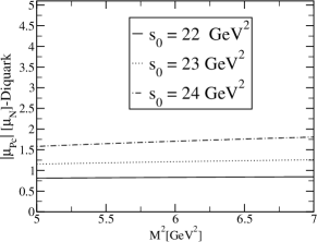
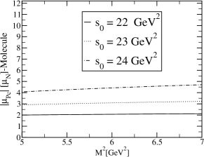
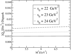
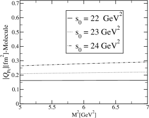
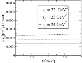
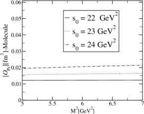
Figure 1: The dependence of the magnetic dipole, electric quadrupole and magnetic octupole moments for $P_{c}$ pentaquark; on the Borel parameter squared $M^{2}$ at different fixed values of the continuum threshold.

Our final results for the magnetic dipole, electric quadrupole and magnetic octupole moments are given in Table I. The errors in the given results arise due to the variations in the calculations of the working regions of $M^{2}$ and $s_{0}$ as well as the uncertainties in the values of the input parameters and the photon DAs. We shall remark that the main source of uncertainties is due to the variations of the results with respect to $s_{0}$. As previously mentioned, the continuum threshold is not totally arbitrary but it depends on the energy of the first excited state. We don’t have enough information on the mass of the first excited state in the channel under consideration. Hence we choose its working interval such that the above mentioned criteria of the sum rules be satisfied. Our analyses show that in the selected region for $s_{0}$, the dependence of the results on this parameter is very weak compared to the regions out of its working window. We also would like to note that in Table I and Fig. 1, the absolute values are given since it is not possible to specify the sign of the residue from the mass sum rules. Hence, it is not possible to predict the signs of the magnetic dipole, electric quadrupole and magnetic octupole moments.

Picture	$|\mu_{P_{c}}|[\mu_{N}]$	$|Q_{P_{c}}|[fm^{2}]$	$|O_{P_{c}}|[fm^{3}]$
Diquark	$1.30\pm 0.50$	$0.017\pm 0.05$	$0.0002\pm 0.00006$
Molecule	$3.35\pm 1.35$	$0.23\pm 0.06$	$0.017\pm 0.004$

Table 1: Results of the magnetic dipole, electric quadrupole and magnetic octupole moments of $P_{c}$ pentaquark.

In conclusion, we have calculated the electromagnetic multipole moments of the $P_{c}^{+}(4380)$ pentaquark by modeling it as the diquark-diquark-antiquark and molecular state of $\bar{D}^{*}\Sigma_{c}$ with quantum numbers $J^{P}=\frac{3}{2}^{-}$. The magnetic dipole, electric quadrupole and magnetic octupole moments of this particle have been extracted in the framework of light-cone QCD sum rule. The values of the electromagnetic multipole moments obtained via two pictures show large differences from each other, which can be used to pin down the underlying structure of $P_{c}^{+}(4380)$. In other words, as many models give compatible results on the mass and width with the experimental data preventing us assigning exact inner structure for pentaquarks, the experimental measurement of the electromagnetic multipole moments of the $P_{c}^{+}(4380)$ pentaquark indeed can help us precisely distinguish its inner structure. The electromagnetic multipole moments of $P_{c}^{+}(4380)$ can be extracted through the process $\gamma^{(*)}p\rightarrow P_{c}^{+}(4380)\rightarrow P_{c}^{+}(4380)\,\gamma\rightarrow J/\psi\,p\,\gamma$ like those of $\Delta^{+}$ baryon.

IV Acknowledgements

This work has been supported by the Scientific and Technological Research Council of Turkey (TÜBİTAK) under the Grant No. 115F183.

Appendix A: Explicit forms of the sum rules for $F_{i}^{Di}$

In this appendix, we present the explicit expressions for the sum rules $F_{i}^{Di}$:

$$F_{1}^{Di} =-\frac{e^{m^{2}_{P_{c}}/M^{2}}}{\lambda_{P_{c}}^{2}}\Bigg{\{}\frac{m_{c}\,\langle\bar{q}q\rangle}{3774873\,\pi^{5}}\Bigg{[}-40\,\pi^{2}\,f_{3\gamma}(e_{d}+10e_{u})\,I_{2}[\mathcal{V}]\,I[0,4,4,0]+3(e_{d}+14e_{u})\,I_{4}[\tilde{S}]\,I[0,5,4,0]$$

$$+192\,e_{c}\,\Big{(}I[0,5,2,2]-2\,I[0,5,2,3]+I[0,5,2,4]-2\,I[0,5,3,2]+2\,I[0,5,3,3]+I[0,5,4,2]\Big{)}\Bigg{]}$$

$$-\frac{\langle g_{s}^{2}G^{2}\rangle}{108716359680\,\pi^{7}}\Bigg{[}20\,\pi^{2}\,f_{3\gamma}\Big{(}4\,(32e_{d}+41e_{u})\,I[0,4,4,0]+3\,(9e_{d}+20e_{u})\,I[0,4,5,0]\Big{)}I_{2}[\mathcal{V}]+(72e_{d}+720e_{u}$$

$$-702e_{c})\,I[0,5,2,1]-(324e_{d}+2184e_{u}-2673e_{c})\,I[0,5,2,2]+(492e_{d}+2456e_{u}-3511e_{c})\,I[0,5,2,4]$$

$$-(300e_{d}+1240e_{u}-1811e_{c})\,I[0,5,2,4]+(60e_{d}+248e_{u}-271e_{c})\,I[0,5,2,5]+(216e_{d}+2160e_{u}-2106)$$

$$\times I[0,5,3,1]+(684e_{d}+4728e_{d}-5693e_{c})\,I[0,5,3,2]-(624e_{d}+3424e_{u}-4483e_{c})\,I[0,5,3,3]+(156e_{d}$$

$$+856e_{u}-893e_{c})\,I[0,5,3,4]+(216e_{d}+2160e_{u}-2106e_{c})\,I[0,5,4,1]-(396e_{d}+2904e_{u}-3375e_{c})$$

$$\times I[0,5,4,2]+(132e_{d}+968e_{u}-973e_{c})\,I[0,5,4,3]-(72e_{d}+720e_{u}-702e_{c})\,I[0,5,5,1]+(36e_{d}+360e_{u}$$

$$-351e_{c})\,I[0,5,5,2]\Bigg{]}$$

$$-\frac{f_{3\gamma}}{3019898880\,\pi^{5}}(13e_{d}+58e_{u})\,I_{2}[\mathcal{V}]\,I[0,6,5,0]$$

$$+\frac{e_{c}}{880803840\,\pi^{7}}\Bigg{[}4\,I[0,7,2,3]-13\,I[0,7,2,4]+15\,I[0,7,2,5]-7\,I[0,7,2,6]+I[0,7,2,7]-12\,I[0,7,3,3]$$

$$+27\,I[0,7,3,4]-18\,I[0,7,3,5]+3\,I[0,7,3,6]+12\,I[0,7,4,3]+3\,I[0,7,4,5]-4\,I[0,7,5,3]+I[0,7,5,4]\Bigg{]}\Bigg{\}},$$ (18)

$$F_{2}^{Di} =\frac{m_{P_{c}}\,e^{m^{2}_{P_{c}}/M^{2}}}{\lambda_{P_{c}}^{2}}\Bigg{\{}-\frac{m_{c}\,\langle\bar{q}q\rangle}{125829120\,\pi^{5}}\Bigg{[}-120\,(e_{d}+10e_{u})\,f_{3\gamma}\,\pi^{2}\,I_{2}[\mathcal{V}]\,I[0,4,4,0]+(3e_{d}+14e_{u})I_{4}[\mathcal{S}]+2e_{d}\,I_{4}[\mathcal{T}_{1}]$$

$$\times I[0,5,4,0]+64\,e_{c}\,\Big{(}I[0,5,2,2]-2\,I[0,5,2,3]+I[0,5,2,4]-2\,I[0,5,3,2]+2\,I[0,5,3,3]+I[0,5,4,2]\Big{)}\Bigg{]}$$

$$+\frac{\langle g_{s}^{2}G^{2}\rangle}{108716359680\,\pi^{7}}\Bigg{[}20\,f_{3\gamma}\pi^{2}\,\Big{\{}-4\Big{(}(52e_{d}-19e_{u})I_{2}[\mathcal{A}]-9(32e_{d}+41e_{u})I_{2}[\mathcal{V}]+4(3e_{d}+2e_{u})\,I_{6}[\psi^{\nu}]\Big{)}\,I[0,4,4,0]$$

$$+3\Big{(}8(-34e_{d}+e_{u})I_{2}[\mathcal{A}]+9(9e_{d}+220e_{u})\,I_{2}[\mathcal{V}]\Big{)}\,I[0,4,5,0]\Big{\}}-\Big{\{}(-72e_{d}+702e_{c}-720e_{u})\,I[0,5,2,1]+(324e_{d}$$

$$-2673e_{c}+2184e_{u})\,I[0,5,2,2]+(-492e_{d}+3511e_{c}-2456e_{u})\,I[0,5,2,3]+(300e_{d}-1811e_{c}+1240e_{u})\,I[0,5,2,4]$$

$$+(-60e_{d}+271e_{c}-248e_{u})\,I[0,5,2,5]+(216e_{d}-2106e_{c}+2160e_{u})\,I[0,5,3,1]+(-684e_{d}+5697e_{c}-4728eu)$$

$$\times I[0,5,3,2]+(624e_{d}-4484e_{c}+3424e_{u})\,I[0,5,3,3]+(-156e_{d}+893e_{c}-856e_{u})\,I[0,5,3,4]$$

$$+ (-216e_{d}+2106e_{c}-2160e_{u})\,I[0,5,4,1]+(396e_{d}-3375e_{c}+2904e_{u})\,I[0,5,4,2]+(-132e_{d}+973e_{c}-968e_{u})$$

$$\times I[0,5,4,3]+(72e_{d}-702e_{c}+720e_{u})\,I[0,5,5,1]+(-36e_{d}+351e_{c}-360e_{u})\,I[0,5,5,2]\Big{\}}\Bigg{]}$$

$$+\frac{f_{3\gamma}}{3019898880\,\pi^{5}}(13e_{d}+58e_{u})I_{2}[\mathcal{V}]\,I[0,6,5,0]$$

$$-\frac{e_{c}}{880803840\,\pi^{7}}\Bigg{[}4\,I[0,7,2,3]-13\,I[0,7,2,4]+15\,I[0,7,2,5]-7\,I[0,7,2,6]+I[0,7,2,7]-12\,I[0,7,3,3]$$

$$+27\,I[0,7,3,4]-18\,I[0,7,3,5]+3\,I[0,7,3,6]+12\,I[0,7,4,3]-15\,I[0,7,4,4]+3\,I[0,7,4,5]-4\,I[0,7,5,3]$$

$$+I[0,7,5,4]\Bigg{]}\Bigg{\}},$$ (19)

$$F_{3}^{Di} =\frac{4\,m_{P_{c}}\,e^{m^{2}_{P_{c}}/M^{2}}}{\lambda_{P_{c}}^{2}}\Bigg{\{}\frac{m_{c}\,\langle g_{s}^{2}G^{2}\rangle}{5435817984\,\pi^{7}}\Bigg{[}2\,f_{3\gamma}\,\pi^{2}\,I_{2}[\mathcal{V}]\,\big{(}4\,(5e_{d}-16e_{u})\,I[0,3,3,0]+3\,(3e_{d}+5e_{u})\,I[0,3,4,0]\big{)}+3\,f_{3\gamma}\,\pi^{2}$$

$$\times I_{4}[\mathcal{V}]\,\big{(}14\,(e_{d}+4e_{u})\,I[0,3,3,0]-(9e_{d}+194e_{u})\,I[0,3,4,0]\big{)}(-36e_{d}+351e_{c}-360e_{u})\,I[0,4,1,2]+(108e_{d}$$

$$-977e_{c}+1080e_{u})\,I[0,4,1,3]+(-108e_{d}+901e_{c}-1080e_{u})\,I[0,4,1,4]+(36e_{d}-275e_{c}+360e_{u})\,I[0,4,1,5]$$

$$+(108e_{d}-1053e_{c}+1080e_{u})\,I[0,4,2,2]+(-216e_{d}+1954e_{c}-2160e_{u})\,I[0,4,2,3]+(108e_{d}-901e_{c}+1080e_{u})$$

$$\times I[0,4,2,4]+(-108e_{d}+1053e_{c}-1080e_{u})\,I[0,4,3,2]+(108e_{d}-977e_{c}+1080e_{u})\,I[0,4,3,3]$$

$$+(36e_{d}-351e_{c}+360e_{u})\,I[0,4,4,2]+(-24e_{d}-240e_{u})\,I[1,3,1,3]+(72e_{d}+720e_{u})\,I[1,3,1,4]+(-72e_{d}$$

$$-720e_{u})\,I[1,3,1,5]+(24e_{d}+240e_{u})I[1,3,1,6]+(72e_{d}+720e_{u})\,I[1,3,2,3]+(-144e_{d}-1440e_{u})\,I[1,3,2,4]$$

$$+(72e_{d}+720e_{u})\,I[1,3,2,5]+(-72e_{d}-720e_{u})\,I[1,3,3,3]+(72e_{d}+720e_{u})\,I[1,3,3,4]+(24e_{d}+240e_{u})$$

$$\times I[1,3,4,3]\Bigg{]}$$

$$-\frac{m_{c}\,f_{3\gamma}}{251658240\pi^{5}}\Bigg{[}(e_{d}+4e_{u})\,I_{2}[\mathcal{V}]+6(3e_{d}+14e_{u})\,I_{4}[\mathcal{V}]\Bigg{]}\,I[0,5,4,0]$$

$$+\frac{m_{c}\,e_{c}}{31457280\pi^{7}}\Bigg{[}I[0,6,1,4]-3\,I[0,6,1,5]+3\,I[0,6,1,6]-I[0,6,1,7]-3\,\Big{(}I[0,6,2,4]-2\,I[0,6,2,5]$$

$$+I[0,6,2,6]-I[0,6,3,4]+I[0,6,3,5]\big{)}-I[0,6,4,4]\Bigg{]}\Bigg{\}},$$ (20)

and

$$F_{4}^{Di} =\frac{4\,m^{3}_{P_{c}}\,e^{m^{2}_{P_{c}}/M^{2}}}{\,\lambda_{P_{c}}^{2}}\Bigg{\{}\frac{m_{c}\,\langle g_{s}^{2}G^{2}\rangle}{452984832\pi^{7}}\Bigg{[}3\,f_{3\gamma}\,\pi^{2}\,I_{4}[\mathcal{V}]\Big{(}(3e_{d}-8e_{u})\,I[0,2,3,0]+13e_{u}\,I[0,2,4,0]\Big{)}+4\,(e_{d}+10e_{u})$$

$$\times\Big{(}I[0,3,1,3]-3\,I[0,3,1,4]+3\,I[0,3,1,5]-\,I[0,3,1,6]-3\big{(}I[0,3,2,3]-2\,I[0,3,2,4]+I[0,3,2,5]-I[0,3,3,3]$$

$$+I[0,3,3,4]\big{)}-I[0,3,4,3]\Big{)}\Bigg{]}\Bigg{\}},$$ (21)

where, $m_{c}$ is the mass of the c quark, $e_{q}$ is the electric charge of the corresponding quark, $\langle\bar{q}q\rangle$ and $\langle g_{s}^{2}G^{2}\rangle$ are quark and gluon condensates, respectively.

The functions $I[n,m,l,k]$, $I_{1}[\mathcal{A}]$, $I_{2}[\mathcal{A}]$, $I_{3}[\mathcal{A}]$, $I_{4}[\mathcal{A}]$,  $I_{5}[\mathcal{A}]$, and  $I_{6}[\mathcal{A}]$ are defined as:

$$I[n,m,l,k] =\int_{4m_{c}^{2}}^{s_{0}}ds\int_{0}^{1}dt\int_{0}^{1}dw~{}e^{-s/M^{2}}~{}s^{n}\,(s-4\,m_{c}^{2})^{m}\,t^{l}\,w^{k},$$

$$I_{1}[\mathcal{A}] =\int D_{\alpha_{i}}\int_{0}^{1}dv~{}\mathcal{A}(\alpha_{\bar{q}},\alpha_{q},\alpha_{g})\delta^{\prime}(\alpha_{q}+\bar{v}\alpha_{g}-u_{0}),$$

$$I_{2}[\mathcal{A}] =\int D_{\alpha_{i}}\int_{0}^{1}dv~{}\mathcal{A}(\alpha_{\bar{q}},\alpha_{q},\alpha_{g})\delta^{\prime}(\alpha_{\bar{q}}+v\alpha_{g}-u_{0}),$$

$$I_{3}[\mathcal{A}] =\int D_{\alpha_{i}}\int_{0}^{1}dv~{}\mathcal{A}(\alpha_{\bar{q}},\alpha_{q},\alpha_{g})\delta(\alpha_{q}+\bar{v}\alpha_{g}-u_{0}),$$

$$I_{4}[\mathcal{A}] =\int D_{\alpha_{i}}\int_{0}^{1}dv~{}\mathcal{A}(\alpha_{\bar{q}},\alpha_{q},\alpha_{g})\delta(\alpha_{\bar{q}}+v\alpha_{g}-u_{0}),$$

$$I_{5}[\mathcal{A}] =\int_{0}^{1}du~{}A(u)\delta^{\prime}(u-u_{0}),$$

$$I_{6}[\mathcal{A}] =\int_{0}^{1}du~{}A(u).$$

References

- Nielsen et al. (2010) M. Nielsen, F. S. Navarra, and S. H. Lee, Phys. Rept. 497, 41 (2010), arXiv:0911.1958 [hep-ph] .
- Swanson (2006) E. S. Swanson, Phys. Rept. 429, 243 (2006), arXiv:hep-ph/0601110 [hep-ph] .
- Voloshin (2008) M. B. Voloshin, Prog. Part. Nucl. Phys. 61, 455 (2008), arXiv:0711.4556 [hep-ph] .
- Klempt and Zaitsev (2007) E. Klempt and A. Zaitsev, Phys. Rept. 454, 1 (2007), arXiv:0708.4016 [hep-ph] .
- Godfrey and Olsen (2008) S. Godfrey and S. L. Olsen, Ann. Rev. Nucl. Part. Sci. 58, 51 (2008), arXiv:0801.3867 [hep-ph] .
- Faccini et al. (2012) R. Faccini, A. Pilloni, and A. D. Polosa, Mod. Phys. Lett. A27, 1230025 (2012), arXiv:1209.0107 [hep-ph] .
- Esposito et al. (2015) A. Esposito, A. L. Guerrieri, F. Piccinini, A. Pilloni, and A. D. Polosa, Int. J. Mod. Phys. A30, 1530002 (2015), arXiv:1411.5997 [hep-ph] .
- Chen et al. (2016a) H.-X. Chen, W. Chen, X. Liu, and S.-L. Zhu, Phys. Rept. 639, 1 (2016a), arXiv:1601.02092 [hep-ph] .
- Ali et al. (2017) A. Ali, J. S. Lange, and S. Stone, Prog. Part. Nucl. Phys. 97, 123 (2017), arXiv:1706.00610 [hep-ph] .
- Esposito et al. (2016) A. Esposito, A. Pilloni, and A. D. Polosa, Phys. Rept. 668, 1 (2016), arXiv:1611.07920 [hep-ph] .
- Olsen et al. (2017) S. L. Olsen, T. Skwarnicki, and D. Zieminska, (2017), arXiv:1708.04012 [hep-ph] .
- Lebed et al. (2017) R. F. Lebed, R. E. Mitchell, and E. S. Swanson, Prog. Part. Nucl. Phys. 93, 143 (2017), arXiv:1610.04528 [hep-ph] .
- Aaij et al. (2015) R. Aaij et al. (LHCb), Phys. Rev. Lett. 115, 072001 (2015), arXiv:1507.03414 [hep-ex] .
- Yang and Ping (2017) G. Yang and J. Ping, Phys. Rev. D95, 014010 (2017), arXiv:1511.09053 [hep-ph] .
- Burns (2015) T. J. Burns, Eur. Phys. J. A51, 152 (2015), arXiv:1509.02460 [hep-ph] .
- Lü and Dong (2016) Q.-F. Lü and Y.-B. Dong, Phys. Rev. D93, 074020 (2016), arXiv:1603.00559 [hep-ph] .
- Wang et al. (2016a) G.-J. Wang, R. Chen, L. Ma, X. Liu, and S.-L. Zhu, Phys. Rev. D94, 094018 (2016a), arXiv:1605.01337 [hep-ph] .
- Shimizu and Harada (2017) Y. Shimizu and M. Harada, Phys. Rev. D96, 094012 (2017), arXiv:1708.04743 [hep-ph] .
- Shen et al. (2016) C.-W. Shen, F.-K. Guo, J.-J. Xie, and B.-S. Zou, Nucl. Phys. A954, 393 (2016), arXiv:1603.04672 [hep-ph] .
- Azizi et al. (2017) K. Azizi, Y. Sarac, and H. Sundu, Phys. Rev. D95, 094016 (2017), arXiv:1612.07479 [hep-ph] .
- Roca et al. (2015) L. Roca, J. Nieves, and E. Oset, Phys. Rev. D92, 094003 (2015), arXiv:1507.04249 [hep-ph] .
- Chen et al. (2015a) R. Chen, X. Liu, X.-Q. Li, and S.-L. Zhu, Phys. Rev. Lett. 115, 132002 (2015a), arXiv:1507.03704 [hep-ph] .
- Huang et al. (2016) H. Huang, C. Deng, J. Ping, and F. Wang, Eur. Phys. J. C76, 624 (2016), arXiv:1510.04648 [hep-ph] .
- Meißner and Oller (2015) U.-G. Meißner and J. A. Oller, Phys. Lett. B751, 59 (2015), arXiv:1507.07478 [hep-ph] .
- Xiao and Meißner (2015) C. W. Xiao and U. G. Meißner, Phys. Rev. D92, 114002 (2015), arXiv:1508.00924 [hep-ph] .
- He (2016) J. He, Phys. Lett. B753, 547 (2016), arXiv:1507.05200 [hep-ph] .
- Chen et al. (2015b) H.-X. Chen, W. Chen, X. Liu, T. G. Steele, and S.-L. Zhu, Phys. Rev. Lett. 115, 172001 (2015b), arXiv:1507.03717 [hep-ph] .
- Wang et al. (2016b) G.-J. Wang, L. Ma, X. Liu, and S.-L. Zhu, Phys. Rev. D93, 034031 (2016b), arXiv:1511.04845 [hep-ph] .
- Chen et al. (2016b) R. Chen, X. Liu, and S.-L. Zhu, Nucl. Phys. A954, 406 (2016b), arXiv:1601.03233 [hep-ph] .
- Yamaguchi and Santopinto (2017) Y. Yamaguchi and E. Santopinto, Phys. Rev. D96, 014018 (2017), arXiv:1606.08330 [hep-ph] .
- He (2017) J. He, Phys. Rev. D95, 074004 (2017), arXiv:1607.03223 [hep-ph] .
- Zhu and Qiao (2016) R. Zhu and C.-F. Qiao, Phys. Lett. B756, 259 (2016), arXiv:1510.08693 [hep-ph] .
- Lebed (2015) R. F. Lebed, Phys. Lett. B749, 454 (2015), arXiv:1507.05867 [hep-ph] .
- Anisovich et al. (2015) V. V. Anisovich, M. A. Matveev, J. Nyiri, A. V. Sarantsev, and A. N. Semenova, (2015), arXiv:1507.07652 [hep-ph] .
- Maiani et al. (2015) L. Maiani, A. D. Polosa, and V. Riquer, Phys. Lett. B749, 289 (2015), arXiv:1507.04980 [hep-ph] .
- Ghosh et al. (2015) R. Ghosh, A. Bhattacharya, and B. Chakrabarti, (2015), arXiv:1508.00356 [hep-ph] .
- Wang (2016) Z.-G. Wang, Eur. Phys. J. C76, 70 (2016), arXiv:1508.01468 [hep-ph] .
- Scoccola et al. (2015) N. N. Scoccola, D. O. Riska, and M. Rho, Phys. Rev. D92, 051501 (2015), arXiv:1508.01172 [hep-ph] .
- Liu and Zahed (2017) Y. Liu and I. Zahed, Phys. Rev. D95, 116012 (2017), arXiv:1704.03412 [hep-ph] .
- Guo et al. (2015) F.-K. Guo, U.-G. Meißner, W. Wang, and Z. Yang, Phys. Rev. D92, 071502 (2015), arXiv:1507.04950 [hep-ph] .
- Liu et al. (2016) X.-H. Liu, Q. Wang, and Q. Zhao, Phys. Lett. B757, 231 (2016), arXiv:1507.05359 [hep-ph] .
- Guo et al. (2016) F.-K. Guo, U. G. Meißner, J. Nieves, and Z. Yang, Eur. Phys. J. A52, 318 (2016), arXiv:1605.05113 [hep-ph] .
- Bayar et al. (2016) M. Bayar, F. Aceti, F.-K. Guo, and E. Oset, Phys. Rev. D94, 074039 (2016), arXiv:1609.04133 [hep-ph] .
- Lin et al. (2017) Y.-H. Lin, C.-W. Shen, F.-K. Guo, and B.-S. Zou, Phys. Rev. D95, 114017 (2017), arXiv:1703.01045 [hep-ph] .
- Eides et al. (2018) M. I. Eides, V. Yu. Petrov, and M. V. Polyakov, Eur. Phys. J. C78, 36 (2018), arXiv:1709.09523 [hep-ph] .
- Azizi et al. (2018) K. Azizi, Y. Sarac, and H. Sundu, (2018), arXiv:1802.01384 [hep-ph] .
- Park et al. (2017) W. Park, A. Park, S. Cho, and S. H. Lee, Phys. Rev. D95, 054027 (2017), arXiv:1702.00381 [hep-ph] .
- Ortega et al. (2017) P. G. Ortega, D. R. Entem, and F. Fernández, Phys. Lett. B764, 207 (2017), arXiv:1606.06148 [hep-ph] .
- Shimizu et al. (2016) Y. Shimizu, D. Suenaga, and M. Harada, Phys. Rev. D93, 114003 (2016), arXiv:1603.02376 [hep-ph] .
- Chen et al. (2016c) H.-X. Chen, E.-L. Cui, W. Chen, X. Liu, T. G. Steele, and S.-L. Zhu, Eur. Phys. J. C76, 572 (2016c), arXiv:1602.02433 [hep-ph] .
- Kim and Praszalowicz (2004) H.-C. Kim and M. Praszalowicz, Phys. Lett. B585, 99 (2004), arXiv:hep-ph/0308242 [hep-ph] .
- Huang et al. (2004) P.-Z. Huang, W.-Z. Deng, X.-L. Chen, and S.-L. Zhu, Phys. Rev. D69, 074004 (2004), arXiv:hep-ph/0311108 [hep-ph] .
- Liu et al. (2004) Y. R. Liu, P. Z. Huang, W. Z. Deng, X. L. Chen, and S.-L. Zhu, Phys. Rev. C69, 035205 (2004), arXiv:hep-ph/0312074 [hep-ph] .
- Wang et al. (2005) Z.-G. Wang, W.-M. Yang, and S.-L. Wan, J. Phys. G31, 703 (2005), arXiv:hep-ph/0503073 [hep-ph] .
- Wang et al. (2006) Z.-G. Wang, S.-L. Wan, and W.-M. Yang, Eur. Phys. J. C45, 201 (2006), arXiv:hep-ph/0503007 [hep-ph] .
- Bijker et al. (2004) R. Bijker, M. M. Giannini, and E. Santopinto, Phys. Lett. B595, 260 (2004), arXiv:hep-ph/0403029 [hep-ph] .
- Li et al. (2004) W. W. Li, Y. R. Liu, P. Z. Huang, W. Z. Deng, X. L. Chen, and S.-L. Zhu, HEPNP 28, 918 (2004), arXiv:hep-ph/0312362 [hep-ph] .
- Chernyak and Zhitnitsky (1990) V. L. Chernyak and I. R. Zhitnitsky, Nucl. Phys. B345, 137 (1990).
- Braun and Filyanov (1989) V. M. Braun and I. E. Filyanov, Z. Phys. C44, 157 (1989), [Yad. Fiz.50,818(1989)].
- Balitsky et al. (1989) I. I. Balitsky, V. M. Braun, and A. V. Kolesnichenko, Nucl. Phys. B312, 509 (1989).
- Weber and Arenhovel (1978) H. J. Weber and H. Arenhovel, Phys. Rept. 36, 277 (1978).
- Nozawa and Leinweber (1990) S. Nozawa and D. B. Leinweber, Phys. Rev. D42, 3567 (1990).
- Pascalutsa et al. (2007) V. Pascalutsa, M. Vanderhaeghen, and S. N. Yang, Phys. Rept. 437, 125 (2007), arXiv:hep-ph/0609004 [hep-ph] .
- Ramalho et al. (2009) G. Ramalho, M. T. Pena, and F. Gross, Phys. Lett. B678, 355 (2009), arXiv:0902.4212 [hep-ph] .
- Azizi (2009) K. Azizi, Eur. Phys. J. C61, 311 (2009), arXiv:0811.2670 [hep-ph] .
- Aliev et al. (2009) T. M. Aliev, K. Azizi, and M. Savci, Phys. Lett. B681, 240 (2009), arXiv:0904.2485 [hep-ph] .
- Belyaev and Ioffe (1983) V. M. Belyaev and B. L. Ioffe, Sov. Phys. JETP 57, 716 (1983), [Zh. Eksp. Teor. Fiz.84,1236(1983)].
- Balitsky and Braun (1989) I. I. Balitsky and V. M. Braun, Nucl. Phys. B311, 541 (1989).
- Ball et al. (2003) P. Ball, V. M. Braun, and N. Kivel, Nucl. Phys. B649, 263 (2003), arXiv:hep-ph/0207307 [hep-ph] .
- Patrignani et al. (2016) C. Patrignani et al. (Particle Data Group), Chin. Phys. C40, 100001 (2016).
- Ioffe (2006) B. L. Ioffe, Prog. Part. Nucl. Phys. 56, 232 (2006), arXiv:hep-ph/0502148 [hep-ph] .