Generalized Hermite Polynomials and Monodromy-Free Schrödinger Operators

Generalized Hermite Polynomials
and Monodromy-Free Schrödinger Operators

Victor Yu. NOVOKSHENOV

V.Yu. Novokshenov

Institute of Mathematics, Russian Academy of Sciences,
112 Chernyshevsky Str., 450008, Ufa, Russia novik53@mail.ru http://matem.anrb.ru/ru/novokshenovvy

Received March 20, 2018, in final form September 20, 2018; Published online September 30, 2018

The paper gives a review of recent progress in the classification of monodromy-free Schrödinger operators with rational potentials. We concentrate on a class of potentials constituted by generalized Hermite polynomials. These polynomials defined as Wronskians of classic Hermite polynomials appear in a number of mathematical physics problems as well as in the theory of random matrices and 1D SUSY quantum mechanics. Being quadratic at infinity, those potentials demonstrate localized oscillatory behavior near the origin. We derive an explicit condition of non-singularity of the corresponding potentials and estimate a localization range with respect to indices of polynomials and distribution of their zeros in the complex plane. It turns out that 1D SUSY quantum non-singular potentials come as a dressing of the harmonic oscillator by polynomial Heisenberg algebra ladder operators. To this end, all generalized Hermite polynomials are produced by appropriate periodic closure of this algebra which leads to rational solutions of the Painlevé IV equation. We discuss the structure of the discrete spectrum of Schrödinger operators and its link to the monodromy-free condition.

generalized Hermite polynomials; monodromy-free Schrödinger operator; Painlevé IV equation; meromorphic solutions; distribution of zeros; 1D SUSY quantum mechanics

30D35; 30E10; 33C75; 34M35; 34M55; 34M60

In memory of my friend and colleague Andrei Kapaev

1 Introduction

The integrability property of Painlevé equations reveals a number of applications of their solutions. Besides traditional self-similar modes in nonlinear PDE’s of mathematical physics they provide new construction material for integrable quantum mechanics and spectral theory. In this paper, we give a brief review of recent achievements in these applications of rational solutions of the fourth Painlevé equation (PIV). We trace how they come from monodromy-free potentials of the Schrödinger equation and from supersymmetric dressing of the harmonic potential in one-dimensional quantum mechanics.

Another ingredients of these interconnections are the generalized Hermite polynomials which build all rational solutions of PIV. Their appearance in multiple applications is explained by the determinant representation of these polynomials. Actually, it can be set as a definition in terms of classical Hermite polynomials. Namely, generalized Hermite polynomials (GHP) $H_{m,n}(z)$ are defined as follows [8, 19]

$$H_{m,n}(z)=\det\left(P_{n-i+j}(z)\right)_{i,j=1}^{m},$$

where

$$P_{s}(z)=\sum_{i+2j=s}\frac{1}{6^{j}i!j!}z^{i},$$

or, equivalently, as Wronskians of classical Hermite polynomials

$$H_{m,n}(z)=c_{m,n}{\mathcal{W}}\left(H_{m}(z),H_{m+1}(z),\ldots,H_{{{m+n-1}}}(z)\right),$$ (1.1)

where $H_{n}(z)=(-1)^{n}{\rm e}^{z^{2}}\frac{{\rm d}^{n}}{{\rm d}z^{n}}{\rm e}^{-z^{2}}$ and $c_{m,n}$ are normalization constants.

Like classical orthogonal polynomials $H_{m,n}$ have a number of useful properties. For example, they constitute recurrence coefficients for orthogonal polynomials $p_{n}(x)$ with weight $w(x,z,m)=(x-z)^{m}\exp\big{(}{-}x^{2}\big{)}$ [7, 10]

$$xp_{n}(x)=p_{n+1}(x)+a_{n}(z,m)p_{n}(x)+b_{n}(z,m)p_{n-1}(x),$$

where

$$a_{n}(z,m)=-\frac{1}{2}\frac{{\rm d}}{{\rm d}z}\ln\frac{H_{n+1,m}}{H_{n,m}},\qquad b_{n}(z,m)=\frac{nH_{n+1,m}H_{n-1,m}}{2H^{2}_{n,m}}.$$

Another property is a formula for rational solutions to the Painlevé IV equation

$$v(z)={-2z+}\frac{{\rm d}}{{\rm d}z}\ln\frac{H_{{m,n+1}}(z)}{H_{{m+1,n}}(z)}.$$ (1.2)

In this case PIV equation

$$v^{\prime\prime}=\frac{(v^{\prime})^{2}}{2v}+\frac{3}{2}v^{3}+4zv^{2}+2\big{(}z^{2}-a\big{)}v+{\frac{b}{v}},$$ (1.3)

has integer coefficients

$$a=n-m,\qquad b=-2(m+n+1)^{2},$$

where $m$ and $n$ are the indices of the corresponding polynomials [16].

The solutions (1.2) have a specific structure of poles in the complex plane. It can be thought of as an equilibrium state of Coulomb charged particles in an external field. Indeed, any pole of a rational solution to PIV has residue equal to $c_{j}=+1$ or $c_{j}=-1$ (see Theorem 3.1). The poles $z_{j}$ can be interpreted as positive and negative charges interacting by the logarithmic potential and influenced by the external quadratic potential

$$U(z_{1},z_{2},\ldots,z_{n})=\sum\limits_{j=1}^{n}c_{j}z_{j}^{2}+\sum\limits_{j\not=k}^{n}c_{j}c_{k}\log(z_{j}-z_{k})^{2}.$$

The equilibrium condition provides the generalized Stiltjes relation [25]

$$\sum\limits_{j\not=k}\frac{c_{j}}{z_{k}-z_{j}}+z_{k}=0,\qquad k=1,2,\ldots.$$

Here each pole coincides with zero of the related polynomial. The distribution of poles for large orders of polynomials has been studied since classical works by T. Stiltjes [24] and M. Plancherel and W. Rotach [22]. This question was discussed recently in applications to dynamics of Coulomb log-gases [14] and approximations by rational functions in logarithmic potential theory [23].

Since the PIV equation (1.3) is integrable in the sense of soliton theory [13, 15], all its rational solutions have been found and labeled by recursions of Bäcklund transformations [13, Chapter 6]. These recursions can be rewritten as dressing chains of the Lax operator with some periodic closures. As a by-product this gives a set of Schrödinger operators $L$ formed by GHP

$$L=-\frac{{\rm d}^{2}}{{\rm d}x^{2}}+u(x),\qquad u(x)=f^{\prime}(x)+f^{2}(x),\qquad f(x)=-x+\frac{{\rm d}}{{\rm d}z}\ln\frac{H_{m,n}(z)}{H_{m,n+1}(z)}.$$ (1.4)

These operators are monodromy-free (see Section 2) and the discrete spectrum of each is an arithmetic sequence with a finite gap (Theorem 3.7). Moreover, all potentials (1.4) are non-singular on the real line for odd $n$. This is due to Theorem 3.5 below which proves $\operatorname{Res}u(z)=0$. In turn, this follows from the distribution of zeros of GHP.

One can mention also a recent application of GHP in matrix models of statistical physics. Consider a degenerate Gaussian unitary ensemble where eigenvalues $\lambda_{k}$ are fixed $k=1,2,\ldots,n$, and $\lambda_{n+1}=z$ has $m$-fold multiplicity. Then the partition function of the ensemble has the form [7]

$$D_{n}(z)=\frac{1}{n!}\int^{\infty}_{\infty}\cdots\int^{\infty}_{\infty}\prod_{1\leq i<j\leq n}(\lambda_{i}-\lambda_{j})^{2}\prod\limits_{k=1}^{n}(\lambda_{k}-z)^{m}{\rm e}^{-\lambda_{k}^{2}}{\rm d}\lambda_{k},$$ (1.5)

where

$$D_{n}(z)=A_{m,n}H_{m,n}(cz),\qquad c={\rm i}\sqrt{\frac{2}{3}},\qquad A_{m,n}={\rm const}.$$

Note that formula (1.5) is proved with the help of dressing chains and ladder operators discussed below in Section 4.

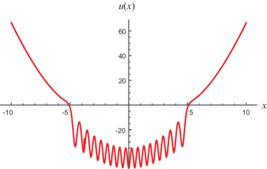
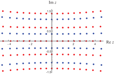
Figure 1: Monodromy-free potential (1.4) $u(x)$, generated by polynomials $H_{m,n}(z)$ and $H_{m,n+1}(z)$ for $m=17$, $n=4$ (left) and zeros of $H_{m,n}$ (blue) and $H_{m,n+1}$ (red) in the complex plane (right).

2 Monodromy-free potentials and dressing chain

A Schrödinger operator

$$L=-\frac{{\rm d}^{2}}{{\rm d}z^{2}}+u(z)$$ (2.1)

with meromorphic potential is called monodromy-free if all solutions of the equation

$$L\psi=-\psi^{\prime\prime}+u\psi=\lambda\psi$$

are meromorphic in the whole complex plane $z\in\mathbb{C}$ for all $\lambda$. In other words, monodromy of the equation (2.1) in the complex plane is trivial for all $\lambda$.

The problem of classification of monodromy-free Schrödinger operators is traditional in spectral theory (see [11, 18]). It became even more important in soliton theory where monodromy-free potentials form a class of soliton solutions to nonlinear equations for which a Schrödinger operator enters the Lax pair. In a case of potentials decreasing at infinity on the real line the spectral theory is well understood (see [28]). In the framework of soliton theory there were found new classes of monodromy-free potentials such as finite-gap ones and rational potentials with quadratic growth at infinity. Here the latter class will be studied in detail in the special case of rational solutions of the PIV equation.

According to [26], the Schrödinger operator (2.1) $L_{j}$ with potential $u_{j}(z)$ is factorized in the form

$$L_{j}=-\left(\frac{{\rm d}}{{\rm d}z}+f_{j}(z)\right)\left(\frac{{\rm d}}{{\rm d}z}-f_{j}(z)\right),$$ (2.2)

where the function $f_{j}(z)$ satisfies the Riccati equation (${}^{\prime}={\rm d}/{\rm d}z$)

$$f_{j}^{\prime}+f_{j}^{2}=u_{j}.$$ (2.3)

The Darboux transformation

$$L_{j}\ \mapsto\ L_{j+1}=-\left(\frac{{\rm d}}{{\rm d}z}-f_{j}(z)\right)\left(\frac{{\rm d}}{{\rm d}z}+f_{j}(z)\right)+\alpha_{j},$$

produces the new potential

$$u_{j+1}=f^{\prime}_{j+1}+f^{2}_{j+1}=-f_{j}^{\prime}+f_{j}^{2}+\alpha_{j}=u_{j}-2f_{j}^{\prime}+\alpha_{j}.$$

This gives rise to the dressing chain equations [26]

$$f^{\prime}_{j+1}+f^{\prime}_{j}=f_{j}^{2}-f_{j+1}^{2}+\alpha_{j},\qquad j=1,2,\ldots,n,\ldots,$$ (2.4)

where $\alpha_{i}$ are arbitrary constants.

In other words, equations (2.4) are equivalent to the relations between Schrödinger operators

$$-\left(\frac{{\rm d}}{{\rm d}z}-f_{j}(z)\right)\left(\frac{{\rm d}}{{\rm d}z}+f_{j}(z)\right)+\alpha_{j}=-\left(\frac{{\rm d}}{{\rm d}z}+f_{j+1}(z)\right)\left(\frac{{\rm d}}{{\rm d}z}-f_{j+1}(z)\right).$$

This property plays a key role in the calculation of spectrum of the monodromy-free potential (2.3) $u(x)=f_{1}^{\prime}(x)+f^{2}_{1}(x)$.

Following [2, 6, 26], consider the following periodic closure of the dressing chain (2.4)

$$f_{j}=f_{j+N},\qquad\alpha_{j}=\alpha_{j+N}.$$

For $N=3$ the infinite chain (2.4) reduces to the second-order ODE written in symmetric form (sPIV) found in [2, 6]

$$\phi^{\prime}_{1}+\phi_{1}(\phi_{2}-\phi_{3})-\alpha_{1}=0,\qquad\phi^{\prime}_{2}+\phi_{2}(\phi_{3}-\phi_{1})-\alpha_{2}=0,$$

$$\phi^{\prime}_{3}+\phi_{3}(\phi_{1}-\phi_{2})-\alpha_{3}=0,$$ (2.5)

where

$$\phi_{1}=f_{1}+f_{2},\qquad\phi_{2}=f_{2}+f_{3},\qquad\phi_{3}=f_{3}+f_{1},$$

and

$$\phi_{1}+\phi_{2}+\phi_{3}=-2z,\qquad\alpha_{1}+\alpha_{2}+\alpha_{3}=-2.$$

The system (2.5), in turn, is equivalent to the PIV equation [2]

$$v^{\prime\prime}=\frac{(v^{\prime})^{2}}{2v}+\frac{3}{2}v^{3}+4zv^{2}+2\big{(}z^{2}-a\big{)}v+{\frac{b}{v}},$$

with

$$v=\phi_{1},\qquad a=\frac{1}{2}(\alpha_{{2}}-\alpha_{{3}}),\qquad b=-\frac{1}{2}\alpha_{1}^{{2}}.$$

The class of rational solutions to the system sPIV has simple “seed solutions”

$$\phi_{1}=-\frac{1}{z},\qquad\phi_{2}=\frac{1}{z},\qquad\phi_{3}=-2z,$$ (2.6)

with parameters $\alpha_{1}=\alpha_{2}={-2}$ and $\alpha_{3}={0}$. They correspond to the “$-1/z$ hierarchy” and the “$-2z$ hierarchy” of PIV rational solutions first found by N. Lukashevich [16]. He proved that there are no other PIV rational solutions with leading terms $-1/z$ or $-2z$ at infinity. Note that there is also a “$-\frac{2}{3}z$” hierarchy of PIV generated by Okamoto polynomials [19] which we will not consider here.

The “$-1/z$” and “$-2z$” hierarchies correspond to rational solutions of the sPIV equation (2.5) formed by generalized Hermite polynomials $H_{m,n}$ [8]

$$\phi_{1}(z)=\frac{{\rm d}}{{\rm d}z}\ln\frac{H_{m+1,n}(z)}{H_{m,n}(z)},\qquad\phi_{2}(z)=\frac{{\rm d}}{{\rm d}z}\ln\frac{H_{m,n}(z)}{H_{m,n+1}(z)},$$

$$\phi_{3}(z)=-2z+\frac{{\rm d}}{{\rm d}z}\ln\frac{H_{m,n+1}(z)}{H_{m+1,n}(z)},$$ (2.7)

where $\alpha_{1}=-2n$, $\alpha_{2}={2m+2n}$, $\alpha_{3}={-2m-2}$.

Due to the symmetry of the sPIV system (2.5) and the periodic relations $f_{j}=f_{j+3}$ the first dressing chain component takes the form

$$f^{(1)}_{1}(z)=-z-\frac{{\rm d}}{{\rm d}z}\ln\frac{H_{m,n}(z)}{H_{m,n+1}(z)},\qquad f^{(2)}_{1}(z)=z+\frac{{\rm d}}{{\rm d}z}\ln\frac{H_{m+1,n}(z)}{H_{m,n+1}(z)},$$

$$f^{(3)}_{1}(z)=-z{+}\frac{{\rm d}}{{\rm d}z}\ln\frac{H_{m,n}(z)}{H_{m+1,n}(z)}.$$ (2.8)

Note that formulas (2.8) can be derived also from results of A. Oblomkov [21]. He proved that any monodromy-free potential of a Schrödinger operator (2.2) with

$$f_{j}=\sum\limits_{k=1}^{N}\frac{c_{k}}{z-z_{k}}-z$$

is quadratic at infinity and has the form

$$u(z)=z^{2}-2\frac{{\rm d}^{2}}{{\rm d}z^{2}}\ln\mathcal{W}(H_{m}(z),H_{m+1}(z),\ldots,H_{m+n{-1}}(z)),$$ (2.9)

where $\mathcal{W}$ is the Wronskian and $H_{k}$ are classical Hermite polynomials. This form of the potential can easily be derived from the definition $u=f_{1}^{\prime}+f_{1}^{2}$ by using relations (2.8)

$$u(z)=z^{2}-2\frac{{\rm d}^{2}}{{\rm d}z^{2}}\ln H_{m+1,n}(z)+2n-1,$$ (2.10a)

$$u(z)=z^{2}-2\frac{{\rm d}^{2}}{{\rm d}z^{2}}\ln H_{m,n+1}(z)+2n-2m+1,$$ (2.10b)

$$u(z)=z^{2}-2\frac{{\rm d}^{2}}{{\rm d}z^{2}}\ln H_{m,n}(z)-2m-1.$$ (2.10c)

Taking into account the definition (1.1) we come to the representation (2.9) up to a constant term.

3 Non-singular potentials on the real line

Spectral theory of Schrödinger operators (2.2) usually supposes a potential $u(x)$ being non-singular, i.e., belonging to some functional space like $L_{2}(\mathbb{R})$. This is true especially for applications like quantum mechanics as we will discuss in Section 4.

We begin with the structure of poles of rational PIV solutions (2.8). In general, all solutions of (1.3) are meromorphic functions. They are described by the following

Theorem 3.1 ([25]).

Any rational solution to equation (1.3) has the form

$$v(z)=\epsilon z+\sum\limits_{j}\frac{c_{j}}{z-z_{j}},\qquad\epsilon=0,-\frac{2}{3},-2,\qquad c_{j}=\pm 1,\qquad j=1,2,\ldots,$$ (3.1)

and the generalized Stieltjes relation is true

$$\sum\limits_{j\not=k}\frac{c_{j}}{z_{k}-z_{j}}+(\epsilon+1)z_{k}=0,\qquad k=1,2,\ldots.$$ (3.2)

Proof.

Take a Laurent series near a pole $z=z_{j}$

$$v(z)=\sum\limits_{k=-l}^{\infty}c_{k}(z-z_{j})^{k},\qquad z\to z_{j}.$$ (3.3)

Balancing the leading terms of the series in equation (1.3) yield $l=1$, $c_{-1}^{2}=1$. A similar comparison at infinity proves that rational solution $u(z)$ has at most linear growth $u(z)=\epsilon z+O(1)$ as $z\to\infty$ with $\epsilon=0,-2/3,-2$. Expand a rational solution $u(z)$ into simple fractions (3.1) and put it into equation (1.3) looking for terms of order $O(z-z_{k})^{-2}$ as $z\to z_{k}$. Balancing these terms gives the relations (3.2) for any pole $z_{k}$. ∎

Corollary 3.2.

For any solution $v$ of the PIV equation (1.3) the residues of the function $(z+v(z))^{2}$ are zero at any pole $z=z_{k}$

$$\operatorname{Res}(z+v(z))^{2}=0.$$

Proof.

From the Laurent series (3.3) one easily derives $c_{0}=-z_{j}$. This yields the similar asymptotics for $z+v(z)$

$$z+v(z)=\frac{c_{-1}}{z-z_{j}}+(c_{0}+z_{j})+(c_{1}+1)(z-z_{j})+\cdots$$

$$\hphantom{z+v(z)}{}=\frac{c_{-1}}{z-z_{j}}+(c_{1}+1)(z-z_{j})+\cdots.$$ ∎

Each pole of the functions (2.8) comes from a zero of a GHP $H_{m,n}$, $H_{m,n+1}$ or $H_{m+1,n}$. The polynomials satisfy the recurrence relations [8]

$$2mH_{m+1,n}H_{m-1,n}=H_{m,n}H^{\prime\prime}_{m,n}-(H^{\prime}_{m,n})^{2}+2mH^{2}_{m,n},$$

$$2nH_{m,n+1}H_{m,n-1}=-H_{m,n}H^{\prime\prime}_{m,n}+(H^{\prime}_{m,n})^{2}+2nH^{2}_{m,n},$$ (3.4)

with initial conditions

$$H_{0,0}=H_{0,1}=H_{1,0}=1,\qquad H_{1,1}=2z.$$

One can easily prove by induction that solutions of the system (3.4) are polynomials and each $H_{m,n}$ has $mn$ simple zeros. Due to the obvious symmetries

$$H_{m,n}(-z)=(-1)^{mn}H_{m,n}(z),\qquad H_{m,n}({\rm i}z)={\rm i}^{mn}H_{{n,m}}(z),$$

all zeros form a symmetric pattern with respect to real and imaginary axes.

Note that $H_{m,1}=H_{m}$, where $H_{m}$ is the classical Hermite polynomial of $m$-th order, $H_{m}(z)=(-1)^{m}{\rm e}^{z^{2}}\frac{{\rm d}^{m}}{{\rm d}z^{m}}{\rm e}^{-z^{2}}$. This means that all zeros of $H_{m,1}$ are on the real line. However, all polynomials $H_{m,n}$ with even $n$ do not have any real-valued zeroes. This follows from the theorem of V.E. Adler

Theorem 3.3 ([1]).

For $x\in\mathbb{R}$ all Wronskians ${\mathcal{W}}(H_{m_{1}}(x),H_{m_{2}}(x),\ldots,H_{m_{n}}(x))\not=0$ if $m_{1}<m_{2}<\dots<m_{n}$ and $n$ is even.

The typical pattern of zeros is a slightly deformed rectangular region shown in Fig. 1 (right). Its horizontal and vertical ranges are proportional to $\sqrt{2m+n}$ and $\sqrt{2n+m}$ respectively. Recently, the generalized Hermite polynomials have been studied in the limit $m,n\to\infty$ in a number of papers [5, 12, 17, 20]. In the paper [17], the distribution of zeros of $H_{m,n}(z)$ was obtained in the asymptotic limit $m\to\infty$, $n=O(1)$. On the other hand, the paper [5] contains an analysis of $H_{m,n}(z)$ in the limit $m,n\to\infty$, $m=rn$, $r=O(1)$ and deduces in particular bounds for the deformed rectangular region containing the zeros. The asymptotic distribution of zeros in the latter asymptotic regime, i.e., the generalization of Plancherel–Rotach formulas to $H_{m,n}(z)$ for $z$ within the deformed rectangular region for $m$ and $n$ of similar large order, remains an open problem. We note that both papers [5, 17] apply methods of asymptotic “undressing” of Riemann–Hilbert problems.

Remark 3.4.

Note that in [5] a mistake was corrected in the asymptotics found in [20]. Namely, there was an incorrect leading term of the Riemann surface equation which led to genus-0 functions instead of genus-1 functions responsible for the asymptotic distribution of zeros. In turn, the poles near each vertex of the asymptotic “rectangle” (see Fig. 1 right) were found incorrectly.

We now prove that the potentials $u(z)$ provided by (2.8) are non-singular on the real line.

Theorem 3.5.

The potential $u(x)=f^{\prime}_{1}(x)+f_{1}^{2}(x)$ is non-singular at $x\in\mathbb{R}$ if

$$f_{1}=f^{(1)}_{1},\qquad n=2k,$$ (3.5a)

$$f_{1}=f^{(2)}_{1},\qquad n=2k+1,$$ (3.5b)

$$f_{1}=f^{(3)}_{1},\qquad n=2k,$$ (3.5c)

and $m$ is arbitrary.

Proof.

Note that the functions (2.8) $f_{1}$ can be written as

$$f_{1}(z)=-z-v(z),$$

with $v=\phi_{j+1}$ as $f_{1}=f_{1}^{(j)}$, $j=1,2,3$, $\phi_{4}=\phi_{1}$.

Then, by Corollary 3.2,

$$f_{1}^{2}=(z+v(z))^{2}=\frac{c^{2}_{-1}}{(z-z_{j})^{2}}+O(1),\qquad z\to z_{j}$$

for every pole $z=z_{j}$ of $v$. This yields

$$u=f_{1}^{\prime}+f_{1}^{2}=\frac{-c_{-1}+c^{2}_{-1}}{(z-z_{j})^{2}}+O(1),\qquad z\to z_{j}.$$

By Theorem 3.1, $c_{-1}=\pm 1$, and the pole of $u$ vanishes only for $c_{-1}=1$. Since all GHP have simple zeros, $H_{i,j}(z)=a(z-z_{1})\cdots(z-z_{ij})$, we have

$$c_{-1}=\mathop{\rm Res}\limits_{z=z_{j}}\frac{{\rm d}}{{\rm d}z}\ln\frac{H_{m+1,n}(z)}{H_{m,n+1}(z)}=\begin{cases}\hphantom{-}1,&H_{m+1,n}(z_{j})=0,\\ -1,&H_{m,n+1}(z_{j})=0,\end{cases}$$

Thus one should eliminate real-valued zeros $z_{j}\in\mathbb{R}$ that provide $c_{-1}=-1$, i.e., the real-valued zeros of denominators in (2.7).

As for the cases (3.5a) and (3.5c), the denominators in (2.7) are $H_{m,n}$ and $H_{m+1,n}$ respectively. If $n=2k$ those polynomials do not have real-valued zeros due to Theorem 3.3. The real-valued zeros of $H_{m,n+1}$ in this case provide residues $c_{-1}=1$, so that $u=f_{1}^{\prime}+f_{1}^{2}$ is non-singular.

In the case (3.5b) we have $n=2k+1$ which yields the denominator $H_{m,n+1}$ to have no zeros on the real line. Here the zeros of the numerator provide residues $c_{-1}=1$, and $u=f_{1}^{\prime}+f_{1}^{2}$ again is non-singular. ∎

Remark 3.6.

The statement of Theorem 3.5 is in line with the representation (2.9) of the potential $u(x)$ by A. Oblomkov [21]. Due to Theorem 3.3 the logarithmic derivatives in (2.10) are non-singular if $n$ is even in cases a) and c) and $n$ is odd in case b).

We now discuss the spectrum of Schrödinger operators (2.2) with non-singular potentials (2.3)

$$L\psi=\lambda\psi,\qquad L=-\left(\frac{{\rm d}}{{\rm d}x}+f\right)\left(\frac{{\rm d}}{{\rm d}x}-f\right)=-\frac{{\rm d}^{2}}{{\rm d}x^{2}}+u(x).$$

All potentials $u$ are quadratic at infinity. Note that the quadratic potential itself $u(x)=x^{2}-1$ has discrete spectrum which is the set of even numbers, $\operatorname{Sp}\big{(}{-}\frac{{\rm d}^{2}}{{\rm d}x^{2}}+x^{2}-1\big{)}=\{\lambda_{k}=2k,\,k=0,1,\ldots\}$. Actually, the GHP potentials demonstrate similar features.

Theorem 3.7.

If the operator $L$ has potentials (2.3) $u=f^{\prime}+f^{2}$ with $f=f_{1}^{(j)}$, $j=1,2,3$ in (2.8), then its spectrum is discrete and consists of even numbers with the exception or addition of a finite number of terms

$$\operatorname{Sp}(L)=\{\lambda=2k,\,k=0,1,\ldots,m,m+n+1,\ldots\},$$ (3.6a)

$$\operatorname{Sp}(L)=\{\lambda=2k,\,k=-m,-m+1,\ldots,0,n+1,n+2,\ldots\},$$ (3.6b)

$$\operatorname{Sp}(L)=\{\lambda=2k,\,k=-m-n,-m-n+1,\ldots,-n-1,0,1,\ldots\}.$$ (3.6c)

Proof.

Since all potentials (2.3) came from iterations of Darboux transformations by the dressing chain (2.4), their spectra are computed explicitly by M. Crum’s method [9]. Namely, if the potential $u_{1}$ has discrete spectrum with eigenfunctions $\psi_{k}$ corresponding to distinct $\lambda_{k}$, $k=1,2,\ldots$, then $n$-th Darboux iteration $u_{n}$ has the form

$$u_{n}(z)=u_{1}(z)-2\frac{{\rm d}^{2}}{{\rm d}z^{2}}\ln\mathcal{W}(\psi_{1}(z),\ldots,\psi_{n}(z)),$$

and its eigenfunctions are

$$\psi_{n,k}=\frac{\mathcal{W}(\psi_{1},\ldots,\psi_{n},\psi_{k})}{\mathcal{W}(\psi_{1},\ldots,\psi_{n})},\qquad k>n.$$ (3.7)

Here $n$ should be even, else the denominator in (3.7) has real-valued zeroes and $\psi_{n,k}$ have non-integrable singularities. Since $\psi_{1},\ldots,\psi_{n}$ are no longer eigenfunctions of new potential $u_{n}$, the spectrum of $u_{n}$ coincides with $\operatorname{Sp}\big{(}{-}\frac{{\rm d}^{2}}{{\rm d}x^{2}}+u_{1}\big{)}\setminus\{\lambda_{1},\ldots,\lambda_{n}\}$.

In particular, put $u_{1}=x^{2}-1$ and $\psi_{1}(x)={\rm e}^{-x^{2}/2}H_{m+1}(x),\ldots,\psi_{n}(x)={\rm e}^{-x^{2}/2}H_{m+n}(x)$, where $H_{k}$ are classical Hermite polynomials. Then

$$u_{n}(z)=z^{2}-2\frac{{\rm d}^{2}}{{\rm d}z^{2}}\ln\mathcal{W}(H_{m+1}(z),\ldots,H_{m+n})+2n-1$$

$$\hphantom{u_{n}(z)}{}=z^{2}-2\frac{{\rm d}^{2}}{{\rm d}z^{2}}\ln H_{m+1,n}(z)+2n-1,$$

which follows from the representation (2.10a). Since $\operatorname{Sp}\big{(}{-}\frac{{\rm d}^{2}}{{\rm d}x^{2}}+x^{2}-1\big{)}=2\mathbb{N}$ and $\lambda_{k}=2(m+k)$, we come to formula (3.6a).

The other two cases (3.6b) and (3.6c) are proved in a similar way. The spectral gap for the potential (2.10b) is $\{2m,2(m+n)\}$ and the constant shift is $-2m$ with respect to (2.10a). As for (2.10c), the gap is $\{2m,2(m+n-1)\}$ and the constant shift is $-2m-2n$. Applying Crum’s formulas this gives spectra (3.6b) and (3.6c). ∎

Note that the case $f=f_{1}^{(1)}$ and the corresponding spectrum (3.6a) was first found in the paper [1] by V.E. Adler. In the next section we reproduce Theorem 3.7 by the Darboux dressing procedure of the harmonic potential.

4 1D SUSY quantum mechanics and the PIV equation

The idea to factorize quantum Hamiltonians and get supersymmetric potentials dates back to the pioneering paper by E. Witten [27]. Later came examples of one-dimensional realizations of this idea with the simplest polynomial Heisenberg algebras. A connection between the harmonic oscillator and supersymmetric (SUSY) partner potentials generated by this algebra has been long known. Recently these potentials were identified with rational solutions of the PIV equation. Here we follow the papers by D. Bermudes and D.J. Fernández C. [3, 4] describing this application.

Starting with two Schrödinger operators (2.1), say $L_{j}$ and $L_{j+1}$, one can factorize them as shown in Section 2

$$L_{j}=A_{j}^{+}A_{j}^{-}+\epsilon_{j},\qquad L_{j+1}=A_{j}^{-}A_{j}^{+}+\epsilon_{j},$$

where

$$A_{j}^{+}=\frac{{\rm d}}{{\rm d}x}+f_{j}(x),\qquad A_{j}^{-}=\frac{{\rm d}}{{\rm d}x}-f_{j}(x)$$ (4.1)

and $u_{j}\mapsto u_{j}+\epsilon_{j}$, $\alpha_{j}=2(\epsilon_{j}-\epsilon_{j+1})$ in (2.3), (2.4).

Then an intertwining relation holds, namely, $L_{j+1}A_{j}^{+}=A_{j}^{+}L_{j}$ which generates the $k$-th order intertwining operators

$$L_{k}B_{k}^{+}=B_{k}^{+}L_{1},\qquad L_{1}B_{k}^{-}=B_{k}^{-}L_{k},\qquad B_{k}^{+}=A_{k}^{+}\cdots A_{1}^{+},\qquad B_{k}^{-}=A_{1}^{-}\cdots A_{k}^{-}.$$ (4.2)

This represents the standard SUSY algebra

$$[\mathcal{Q}_{a},\mathcal{H}]=0,\qquad\{\mathcal{Q}_{a},\mathcal{Q}_{b}\}=\delta_{ab}\mathcal{H},\qquad a,b=1,2,$$

$$\mathcal{Q}_{1}=\frac{1}{\sqrt{2}}\begin{pmatrix}0&B_{k}^{+}\\ B_{k}^{-}&0\end{pmatrix},\qquad\mathcal{Q}_{2}=\frac{1}{i\sqrt{2}}\begin{pmatrix}0&B_{k}^{+}\\ -B_{k}^{-}&0\end{pmatrix},\qquad\mathcal{H}=\frac{1}{\sqrt{2}}\begin{pmatrix}B_{k}^{+}B_{k}^{-}&0\\ 0&B_{k}^{-}B_{k}^{+}\end{pmatrix}.$$

where $\{\,,\}$ is the anticommutator and $\mathcal{H}$ is the Hamiltonian with superpotential partner $u_{k}=u_{1}+2(f_{1}+\dots+f_{k})^{\prime}$ of the initial potential $u_{1}$ [3].

Similarly, the polynomial Heisenberg algebra for the Hamiltonian (2.1) is formed by the dressing chain operators

$$\big{[}L,B_{k}^{\pm}\big{]}=\pm B_{k}^{\pm},\qquad\big{[}B_{k}^{-},B_{k}^{+}\big{]}=N_{k}(L+I)-N_{k}(L),\qquad N_{k}(L)=\prod_{j=1}^{k}(L-\epsilon_{j}).$$

For $k=3$ this algebra can produce new solutions of the PIV equation starting from the known ones (see [4]). Taking a closure condition $L_{4}=L_{1}-I$ we come to the dressing chain (2.5) with some $\alpha_{1}$, $\alpha_{2}$ and $\alpha_{3}$. An example is given at the end of this section.

First we start with the trivial solution of the “$-2x$ hierarchy” (2.6), which corresponds to the harmonic potential $u_{0}(x)=x^{2}{-1}$. The eigenfunctions of the Schrödinger operator with the harmonic potential

$$L\psi_{0}={2}\epsilon\psi_{0}$$

are written explicitly

$$\psi_{0}(x)=\sqrt{\pi}\big{(}(1-c+{\rm i}(1+c){\rm e}^{{\rm i}\pi\epsilon}\big{)}D_{\epsilon-1}\big{(}\sqrt{2}x\big{)}-2(1+c){\rm e}^{{\rm i}\pi\epsilon/2}\sin(\pi\epsilon)\Gamma(\epsilon)D_{-\epsilon}\big{(}{\rm i}\sqrt{2}x\big{)},\!\!\!$$ (4.3)

where $D_{\nu}(x)$ is the Weber–Hermite function, $\Gamma$ is the gamma function and $c$ is an arbitrary complex-valued constant.

Apply now the ladder operators (4.2) to the basic eigenfunction (4.3). The first SUSY partner potential for $k=1$ to $u_{0}(x)=x^{2}{-1}$ has the form

$$u_{1}(x)=x^{2}-{2}\frac{{\rm d}^{2}}{{\rm d}x^{2}}\ln\psi_{0}(x){-1}.$$

Similarly, the $k$-th potential becomes [3]

$$u_{k}(x)=x^{2}-{2}\frac{{\rm d}^{2}}{{\rm d}x^{2}}\ln\mathcal{W}(\psi_{01},\psi_{02},\ldots,\psi_{0{k}}){-1},$$ (4.4)

where $\mathcal{W}$ is the Wronskian of eigenfunctions (4.3) $\psi_{0j}(x)$ with parameters $\epsilon=\epsilon_{j}$.

This gives a way to construct a set of rational potentials associated with GHP. Take parameters $\epsilon_{j}$ to be integers, because in this case the Weber–Hermite functions in (4.3) become Hermite polynomials multiplied by the exponential ${\rm e}^{-x^{2}/2}$. Namely, if we put

$$\epsilon_{1}=m+1,\qquad\epsilon_{j}=m+j,\qquad c_{j}=-1,\qquad j=2,3,\ldots,n,\qquad m,n\in\mathbb{N},$$

the second term in formula (4.3) vanishes and the potential (4.4) takes the form

$$u_{n}(x)=x^{2}-2\frac{{\rm d}^{2}}{{\rm d}x^{2}}\ln\mathcal{W}\left(H_{m}(x),H_{m+1}(x),\ldots,H_{m+n}(x)\right)+2n-1$$

$$\hphantom{u_{n}(x)}{}=x^{2}-2\frac{{\rm d}^{2}}{{\rm d}x^{2}}\ln H_{m,n+1}(x)+2n-1.$$

Unfortunately, this choice of $\psi_{0}$ leads to singularities in the intermediate eigenfuntions (3.7) of the potential (4.4)

$$\psi_{k,j}=\frac{\mathcal{W}(\psi_{01},\psi_{02},\ldots,\psi_{0j-1})}{\mathcal{W}\left(\psi_{01},\psi_{02},\ldots,\psi_{0j}\right)},\qquad j=2,3,\ldots,k.$$ (4.5)

To avoid this and make the formal dressing procedure correct, we use the following theorem proved by D. Bermudez and D.J. Fernández C. in [4] providing non-singularity of eigenfunctions.

Theorem 4.1.

Schrödinger operators (2.1) with potentials (4.4) are monodromy-free. All potentials (4.4) and eigenfunctions (4.5) are non-singular for $x\in\mathbb{R}$ if the dressing parameters satisfy the conditions

$$\epsilon_{k}<\epsilon_{k-1}<\dots<\epsilon_{1}<0,$$ (4.6)

$$|c_{2j}|<1,\qquad|c_{2j+1}|>1,\qquad j=0,1,\ldots,k,$$ (4.7)

where $\epsilon_{j}=\epsilon$ and $c_{j}=c$ in (4.3).

Proof.

Since the Weber–Hermite functions $D_{\nu}(z)$ in (4.3) are entire functions, so is the Wronskian (4.4). Thus its logarithmic derivative is a meromorphic function. Moreover, any solution $\psi(z,\lambda)$ of the Schrödinger equation with potential (4.4) can be found via a finite dressing chain of $k$ operators $A_{j}^{\pm}$ (4.1), i.e., a finite number of Darboux transformations. This yields trivial monodromy of $\psi(z,\lambda)$.

It is easy to check that the function (4.3) has no real-valued zeros if $\epsilon<0$ and $|c|<1$. The remaining inequalities (4.6) and (4.7) are proved by induction (see [3] for details). ∎

Apply now Theorem 4.1 to get non-singular functions (4.5). Take parameters $\epsilon_{j}$ and $c_{j}$ in the form

$$\epsilon_{1}=-n,\!\!\qquad\epsilon_{j}=-n-j,\!\!\qquad c_{2j}=0,\!\!\qquad c_{2j-1}=\infty,\!\!\qquad j=1,2,\ldots,m-1,\!\!\qquad m,n\in\mathbb{N}.$$

In the case of odd $j$ the eigenfunctions (4.3) are normalized as $\psi_{0j}=D_{-\epsilon}\big{(}{\rm i}\sqrt{2}x\big{)}$. This forces the first term in (4.3) to be zero while the second term turns into the Hermite polynomial ${\rm e}^{x^{2}/2}H_{n+j}({\rm i}x)$. Thus the potential (4.4) becomes

$$u_{n}(x)=x^{2}-2\frac{{\rm d}^{2}}{{\rm d}x^{2}}\ln\mathcal{W}(H_{n}({\rm i}x),H_{n+1}({\rm i}x),\ldots,H_{n+m-1}({\rm i}x))-2m-1$$

$$\hphantom{u_{n}(x)}{}=x^{2}-2\frac{{\rm d}^{2}}{{\rm d}x^{2}}\ln H_{m,n}(x)-2m-1,$$ (4.8)

because $H_{k,j}({\rm i}x)={\rm i}^{kj}H_{j,k}(x)$.

As shown in [4], the spectrum of the potential (4.8) is

$$\operatorname{Sp}\left(-\frac{{\rm d}^{2}}{{\rm d}x^{2}}+u_{n}\right)=\{2\epsilon_{m-1}-2,\ldots,2\epsilon_{1}-2\}\cup\{0,2,4,\ldots\},$$

which coincides with formula (2.10c) found in Theorem 3.7.

Finally we illustrate the dressing of the “$-2x$ hierarchy” by the ladder operators (4.1), (4.2) with singular eigenfunctions for the case $k=3$

$$B_{3}^{\pm}=\left(\frac{{\rm d}}{{\rm d}x}\pm f_{1}\right)\left(\frac{{\rm d}}{{\rm d}x}\pm f_{2}\right)\left(\frac{{\rm d}}{{\rm d}x}\pm f_{3}\right).$$ (4.9)

The closure condition $L_{4}=L_{1}-I$ leads to the system

$$f_{1}^{\prime}+f_{2}^{\prime}=f_{1}^{2}-f_{2}^{2}-2(\epsilon_{1}-\epsilon_{2}),$$

$$f_{2}^{\prime}+f_{3}^{\prime}=f_{2}^{2}-f_{3}^{2}-2(\epsilon_{2}-\epsilon_{3}),$$

$$f_{3}^{\prime}+f_{1}^{\prime}=f_{3}^{2}-f_{1}^{2}-2(\epsilon_{3}-\epsilon_{1}{-1}),$$

which is equivalent to the sPIV system (2.5), where

$$\alpha_{1}=2(\epsilon_{1}-\epsilon_{2}),\qquad\alpha_{2}=2(\epsilon_{2}-\epsilon_{3}),\qquad\alpha_{3}=2(\epsilon_{3}-\epsilon_{1}{-1}).$$

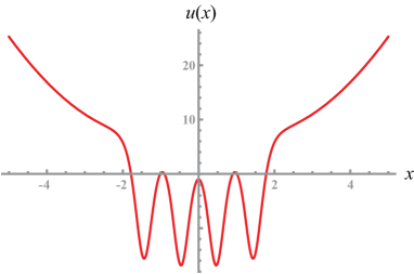
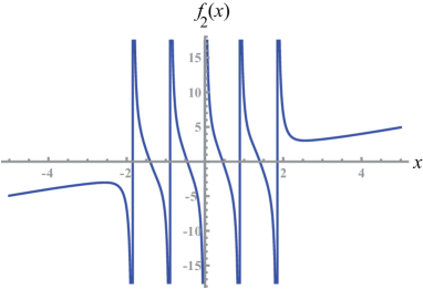
Figure 2: Non-singular potential $u(x)=f_{2}^{\prime}(x)+f^{2}_{2}(x)$ generated by ladder operator (4.9) (left) and its singular component (4.10) $f_{2}(x)$.

Choosing integer values of $\epsilon_{1}$, $\epsilon_{2}$ and $\epsilon_{3}$ it is easy to reproduce the generalized Hermite polynomials which form rational solutions of PIV (2.7). For example, the choice

$${\epsilon_{3}=-3,\qquad\epsilon_{1}=1,\qquad\epsilon_{2}=4,}$$

yields $m=4$ and $n=3$. This provides a rational solution of PIV in the form (2.7)

$$\phi_{2}(x)=\frac{{\rm d}}{{\rm d}x}\ln\frac{H_{4,3}(x)}{H_{4,4}(x)}=\frac{64x^{3}\big{(}7875-900x^{4}+720x^{8}+64x^{1}2\big{)}}{23625+16x^{4}\big{(}7875-450x^{4}+16x^{8}\big{(}15+x^{4}\big{)}\big{)}}$$

$$\hphantom{\phi_{2}(x)=}{}+\frac{24x\big{(}{-}225+2x^{2}\big{(}{-}75-60x^{2}+120x^{4}-40x^{6}+16x^{8}\big{)}\big{)}}{675+4x^{2}\big{(}{-}675-225x^{2}+4x^{4}\big{(}{-}30+45x^{2}-12x^{4}+4x^{6}\big{)}\big{)}}.$$

Since $n$ is odd, by Theorem 3.5 one should choose a non-singular potential from the function (2.8), (3.5b)

$$f_{2}(x)=f_{1}^{(2)}=x+\frac{{\rm d}}{{\rm d}x}\ln\frac{H_{5,3}(x)}{H_{4,4}(x)}$$

$$=x+\frac{1}{x}-\frac{64x^{3}\big{(}7875-900x^{4}+720x^{8}+64x^{12}\big{)}}{23625+16x^{4}\big{(}7875+2x^{4}\big{(}{-}225+8x^{4}\big{(}15+x^{4}\big{)}\big{)}\big{)}}$$ (4.10)

$$\hphantom{=}{}+\frac{4x\big{(}{-}7875+4x^{2}\big{(}{-}4725+2025x^{2}-4200x^{4}+2700x^{6}-720x^{8}+112x^{10}\big{)}\big{)}}{23625+2x^{2}\big{(}{-}7875+2x^{2}\big{(}{-}4725+2x^{2}\big{(}675+2x^{2}\big{(}{-}525+270x^{2}-60x^{4}+8x^{6}\big{)}\big{)}\big{)}\big{)}}.$$

The non-singular potential has the form

$$u(x)=f_{2}^{\prime}(x)+f_{2}^{2}(x)=x^{2}-1+R(x),$$

where $R$ is rational function, $R(x)=O\big{(}x^{-2}\big{)}$, $x\to\infty$. The functions $u$ and $f_{2}$ are plotted in Fig. 2. The spectrum of the Schrödinger operator $L$ with this potential is

$$\operatorname{Sp}(L)=\{-8,-6,-4,-2\}\cup\{8,10,12,\dots\}.$$

Acknowledgements

The work has been supported by Russian Scientific Foundation grant 17-11-01004. The author also is grateful to the referee remarks which helped to improve the paper.

References

• [1] Adler V.E., A modification of Crum’s method, Theoret. and Math. Phys. 101 (1994), 1381–1386.
• [2] Adler V.E., Nonlinear chains and Painlevé equations, Phys. D 73 (1994), 335–351.
• [3] Bermúdez D., Fernández C. D.J., Supersymmetric quantum mechanics and Painlevé IV equation, SIGMA 7 (2011), 025, 14 pages, arXiv:1012.0290.
• [4] Bermúdez D., Fernández C. D.J., Complex solutions to the Painlevé IV equation through supersymmetric quantum mechanics, AIP Conf. Proc. 1420 (2012), 47–51, arXiv:1110.0555.
• [5] Buckingham R., Large-degree asymptotics of rational Painlevé-IV functions associated to generalized Hermite polynomials, Int. Math. Res. Not., to appear, arXiv:1706.09005.
• [6] Bureau F.J., Sur un système d’équations différentielles non linéaires, Acad. Roy. Belg. Bull. Cl. Sci. (5) 66 (1980), 280–284.
• [7] Chen Y., Feigin M.V., Painlevé IV and degenerate Gaussian unitary ensembles, J. Phys. A: Math. Gen. 39 (2006), 12381–12393, math-ph/0606064.
• [8] Clarkson P.A., Special polynomials associated with rational solutions of the Painlevé equations and applications to soliton equations, Comput. Methods Funct. Theory 6 (2006), 329–401.
• [9] Crum M.M., Associated Sturm–Liouville systems, Quart. J. Math. Oxford 6 (1955), 121–127.
• [10] Deift P.A., Orthogonal polynomials and random matrices: a Riemann–Hilbert approach, Courant Lecture Notes in Mathematics, Vol. 3, New York University, Courant Institute of Mathematical Sciences, 1999.
• [11] Duistermaat J.J., Grünbaum F.A., Differential equations in the spectral parameter, Comm. Math. Phys. 103 (1986), 177–240.
• [12] Felder G., Hemery A.D., Veselov A.P., Zeros of Wronskians of Hermite polynomials and Young diagrams, Phys. D 241 (2012), 2131–2137, arXiv:1005.2695.
• [13] Fokas A.S., Its A.R., Kapaev A.A., Novokshenov V.Yu., Painlevé transcendents. The Riemann–Hilbert approach, Mathematical Surveys and Monographs, Vol. 128, Amer. Math. Soc., Providence, RI, 2006.
• [14] Forrester P.J., Log-gases and random matrices, London Mathematical Society Monographs Series, Vol. 34, Princeton University Press, Princeton, NJ, 2010.
• [15] Kapaev A.A., Hubert E., A note on the Lax pairs for Painlevé equations, J. Phys. A: Math. Gen. 32 (1999), 8145–8156.
• [16] Lukaševič N.A., The theory of Painlevé’s fourth equation, Differ. Uravn. 3 (1967), 771–780.
• [17] Masoero D., Roffelsen P., Poles of Painlevé IV rationals and their distribution, SIGMA 14 (2018), 002, 49 pages, arXiv:1707.05222.
• [18] McKean H.P., Trubowitz E., The spectral class of the quantum-mechanical harmonic oscillator, Comm. Math. Phys. 82 (1982), 471–495.
• [19] Noumi M., Yamada Y., Symmetries in the fourth Painlevé equation and Okamoto polynomials, Nagoya Math. J. 153 (1999), 53–86, q-alg/9708018.
• [20] Novokshenov V.Yu., Schelkonogov A.A., Distribution of zeroes to generalized Hermite polynomials, Ufa Math. J. 7 (2015), 54–66.
• [21] Oblomkov A.A., Monodromy-free Schrödinger operators with quadratically increasing potential, Theoret. and Math. Phys. 121 (1999), 374–386.
• [22] Plancherel M., Rotach W., Sur les valeurs asymptotiques des polynomes d’Hermite $H_{n}(x)=(-I)^{n}{\rm e}^{\frac{{x^{2}}}{2}}\frac{{{\rm d}^{n}}}{{{\rm d}x^{n}}}\big{(}{{\rm e}^{-\frac{{x^{2}}}{2}}}\big{)}$, Comment. Math. Helv. 1 (1929), 227–254.
• [23] Saff E.B., Totik V., Logarithmic potentials with external fields, Grundlehren der Mathematischen Wissenschaften, Vol. 316, Springer-Verlag, Berlin, 1997.
• [24] Stieltjes T.J., Sur certains polynômes: qui vérifient une équation différentielle linéaire du second ordre et sur la theorie des fonctions de Lamé, Acta Math. 6 (1885), 321–326.
• [25] Veselov A.P., On Stieltjes relations, Painlevé-IV hierarchy and complex monodromy, J. Phys. A: Math. Gen. 34 (2001), 3511–3519, math-ph/0012040.
• [26] Veselov A.P., Shabat A.B., Dressing chains and the spectral theory of the Schrödinger operator, Funct. Anal. Appl. 27 (1993), 81–96.
• [27] Witten E., Supersymmetry and Morse theory, J. Differential Geom. 17 (1982), 661–692.
• [28] Zakharov V.E., Manakov S.V., Novikov S.P., Pitaevskiĭ L.P., Soliton theory: inverse scattering method, Nauka, Moscow, 1980.
\LastPageEnding