Nonlocal Low-Rank Tensor Factor Analysis for Image Restoration

Abstract

Low-rank signal modeling has been widely leveraged to capture non-local correlation in image processing applications. We propose a new method that employs low-rank tensor factor analysis for tensors generated by grouped image patches. The low-rank tensors are fed into the alternative direction multiplier method (ADMM) to further improve image reconstruction. The motivating application is compressive sensing (CS), and a deep convolutional architecture is adopted to approximate the expensive matrix inversion in CS applications. An iterative algorithm based on this low-rank tensor factorization strategy, called NLR-TFA, is presented in detail. Experimental results on noiseless and noisy CS measurements demonstrate the superiority of the proposed approach, especially at low CS sampling rates.

1 Introduction

Inspired by the nonlocal self-similarity of image patches [3], various image processing algorithms have been proposed to investigate the low-rank property of image patch groups [9, 11, 17, 31, 44]. In general, these methods first select a reference patch and then search for similar patches across the image to form a group. Following this, the patches in this group are vectorized and stacked to a matrix. Since these patches are similar, the constructed matrix has a low-rank property. Via performing this low-rank model on every (overlapping) patch in the image, state-of-the-art image restoration results have been achieved.

One common issue in the above algorithms is that the original two-dimensional (2D) patches are vectorized to construct the group matrix, which loses the spatial structure within the image patch. We propose a tensor based algorithm to retain this structure while still leveraging the advantages of low-rank patch models. Tensor factorization methods [19] offer a useful way to learn latent structure from complex multiway data, and have been used in image processing tasks [43]. These methods decompose the tensor data into a set of factor matrices (one for each mode or “way” of the tensor), that can be used as a latent feature representation for the objects in each of the tensor modes [33]. Recently tensor approaches have been applied in computer vision, such as image denoising [32], and video denoising [42]. We consider the general image restoration problem with specific applications to compressive sensing [12] using the tensor factor analysis (TFA) approach. In particular, instead of vectorizing the image patches, we impose low-rank TFA to the 3D image patch groups.

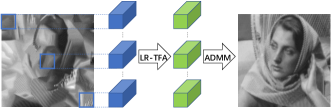
Figure 1: An illustration of the NLR-TFA model. The left image is the initial estimate using some fast algorithm. Each tensor is concatenated by a reference image patch and its similar patches. Blue cubes represent full-rank tensors; green cubes represent low-rank tensors. The right image (PSNR=$26.15$dB) is reconstructed using NLR-TFA from compressive sensing (CS) measurements at a CS rate of only $0.02$. Notice how the proposed method can restore rich semantic content and fine structure of the image, even when the sensing rate is extremely low.

To be concrete, the image restoration problem aims to estimate the latent clean image $\boldsymbol{x}$ given the observation $\boldsymbol{y}$ (the corrupted/compressive measurement) and the measurement matrix $\boldsymbol{\Phi}$, which can be formulated as

$$\boldsymbol{y}=\boldsymbol{\Phi}\boldsymbol{x}+{\boldsymbol{e}},$$ (1)

where ${\boldsymbol{e}}$ denotes the measurement noise and is usually modeled by ${\boldsymbol{e}}\sim\mathcal{N}(0,\sigma^{2}{\bf I})$. The problem has different variants for different $\boldsymbol{\Phi}$: when $\boldsymbol{\Phi}$ is the identity matrix, this is a denoising problem [16]; when $\boldsymbol{\Phi}$ is a diagonal matrix whose diagonal elements are either 1 or 0, keeping or removing corresponding pixels, this becomes image inpainting [63]; and when $\boldsymbol{\Phi}\in\mathbb{C}^{M\times N}$ and $M\ll N$, this is a compressive sensing (CS) problem.

We focus on the CS problem [14, 28], and consider the image reconstruction with a very limited number of compressive measurements [50, 51, 52, 58]. A framework of the proposed NLR-TFA method is shown in Fig. 1. There has been recent interest in using deep learning technique for CS problems [30]. A reconstruction network is developed in [20, 58], and an ADMM-net is proposed in [47]; while the former paper focused on block-wise CS, the latter one only considered CS-MRI [28]. By contrast, we develop a tensor-based framework for general CS applications. Further, to overcome the large-scale matrix inversion in CS, we further propose to pre-train a deep convolutional neural network to approximate the expensive matrix inversion operator [41].

The remainder of this paper is organized as follows. Section 2 presents background knowledge on tensors and CS. Section 3 derives our algorithm. Extensive results are provided in Section 4 to demonstrate the superiority of the proposed algorithm relative to other leading approaches, and Section 5 concludes the paper.

2 Background

2.1 Tensor Decomposition

Tensors (of order higher than two) are arrays indexed by three or more indices. Specifically, matrices are two-way arrays, and tensors are three- or higher-way arrays. In the sequel, we mainly focus on $3\text{-}$way tensors and everything naturally generalizes to higher-order tensors.

A $rank\text{-}1$ $3\text{-}$way tensor $\mathcal{T}\in\mathbb{R}^{I\times J\times K}$ is an outer product of $3$ unit vectors ${\boldsymbol{a}}\in\mathbb{R}^{I}$, ${\boldsymbol{b}}\in\mathbb{R}^{J}$, and ${\boldsymbol{c}}\in\mathbb{R}^{K}$:

$$\mathcal{T} =\lambda{\boldsymbol{a}}\otimes{\boldsymbol{b}}\otimes{\boldsymbol{c}}$$ (2)

$$\mathcal{T}(i,j,k) =\lambda{\boldsymbol{a}}(i){\boldsymbol{b}}(j){\boldsymbol{c}}(k)$$

where $\otimes$ is the vector outer product and $\lambda$ is a scalar.

The $rank$ of a tensor $\mathcal{T}$ is the minimum number of $rank\text{-}1$ tensors that sum to $\mathcal{T}$. Therefore, a $rank\text{-}R$ $3\text{-}$way tensor $\mathcal{T}$ can be written as

$$\mathcal{T} =\sum_{r=1}^{R}\lambda_{r}{\boldsymbol{a}}_{r}\otimes{\boldsymbol{b}}_{r}\otimes{\boldsymbol{c}}_{r}$$ (3)

$$\mathcal{T}(i,j,k) =\sum_{r=1}^{R}\lambda_{r}{\boldsymbol{a}}_{r}(i){\boldsymbol{b}}_{r}(j){\boldsymbol{c}}_{r}(k)$$

where unit vectors ${\boldsymbol{a}}_{r}$, ${\boldsymbol{b}}_{r}$, and ${\boldsymbol{c}}_{r}$ are tensor factors and $\lambda_{r}$ is a scalar that evaluates the significance of tensor factors ${\boldsymbol{a}}_{r},{\boldsymbol{b}}_{r},{\boldsymbol{c}}_{r}$. For brevity, $\mathcal{T}=\sum_{r=1}^{R}\lambda_{r}{\boldsymbol{a}}_{r}\otimes{\boldsymbol{b}}_{r}\otimes{\boldsymbol{c}}_{r}$ can be denoted as $\mathcal{T}=\langle{\boldsymbol{\lambda}},{{\bf A}},{\bf B},{\bf C}\rangle$, where ${\boldsymbol{\lambda}}:=[\lambda_{1},...,\lambda_{R}]$, ${{\bf A}}:=[{\boldsymbol{a}}_{1},...,{\boldsymbol{a}}_{R}]$, ${\bf B}:=[{\boldsymbol{b}}_{1},...,{\boldsymbol{b}}_{R}]$, and ${\bf C}:=[{\boldsymbol{c}}_{1},...,{\boldsymbol{c}}_{R}]$. When the rank $R$ is low, the number of elements needed to represent $\mathcal{T}$ is dramatically decreased after tensor decomposition, i.e., from $I\times K\times J$ to $(I+K+J)\times R$.

Practically, most tensor decomposition problems are NP-hard. However, in most real applications, as long as the tensor does not have too many components, and the components are not adversarially chosen, tensor decomposition can be computed in polynomial time [34]. The tensor-decomposition problem seeks to estimate ${{\bf A}}$, ${\bf B}$, ${\bf C}$ and coefficients ${\boldsymbol{\lambda}}$ from a tensor $\mathcal{T}$. Adopting a least-squares fitness criterion, the problem is

$$\min_{{{\bf A}},{\bf B},{\bf C},{\boldsymbol{\lambda}}}\|\mathcal{T}-\sum_{r=1}^{R}\lambda_{r}{\boldsymbol{a}}_{r}\otimes{\boldsymbol{b}}_{r}\otimes{\boldsymbol{c}}_{r}\|_{F}^{2}$$ (4)

In this work, we employ Jenrich’s algorithm [21] to solve this problem. In Algorithm 1, “$+$” denotes pseudo-inverse of a matrix.

Algorithm 1 Jenrich’s Algorithm

0:  Tensor $\mathcal{T}$.

1:  Pick two random unit vectors $\boldsymbol{u},\boldsymbol{v}$.

2:  Compute $\mathcal{T}_{\boldsymbol{u}}=\sum_{i=1}^{k}u_{i}\mathcal{T}[:,:,i]$;

3:  Compute $\mathcal{T}_{\boldsymbol{v}}=\sum_{i=1}^{k}v_{i}\mathcal{T}[:,:,i]$;

4:  ${\boldsymbol{a}}_{r}$’s are eigenvectors of $\mathcal{T}_{\boldsymbol{u}}(\mathcal{T}_{\boldsymbol{v}})^{+}$, ${\boldsymbol{b}}_{r}$’s are eigenvectors of $(\mathcal{T}_{\boldsymbol{u}}^{\top})(\mathcal{T}_{\boldsymbol{v}}^{\top})^{+}$;

5:  Given ${{\bf A}}$ and ${\bf B}$, we can get ${\boldsymbol{c}}_{r}$’s and $\lambda_{r}$’s by solving a linear system followed by normalization;

6:  Output: Tensor factors ${\boldsymbol{a}}_{r}$’s, ${\boldsymbol{b}}_{r}$’s, ${\boldsymbol{c}}_{r}$’s and coefficients $\lambda_{r}$’s

2.2 Compressive Sensing

Compressive sensing is a signal acquisition technique that enables sampling a signal at sub-Nyquist rates [12]. In CS, a reconstruction algorithm is used to recover the original high-dimensional signal from a small number of random linear measurements. Taking compressive measurements can be viewed as a process of linearly mapping an $N$-dimensional signal vector $\boldsymbol{x}$ to an $M$-dimensional measurement vector $\boldsymbol{y}$, $M\ll N$, using a measurement matrix $\boldsymbol{\Phi}\in\mathbb{C}^{M\times N}$, i.e., $\boldsymbol{y}=\boldsymbol{\Phi}\boldsymbol{x}$. Since the matrix $\boldsymbol{\Phi}$ is rank-deficient, there exists more than one $\boldsymbol{x}$ that yields the same measurement $\boldsymbol{y}$. In this paper, the compressive sensing rate (CSr) is defined as CSr$=M/N$.

To recover $\boldsymbol{x}$, one searches for the vector that possesses a certain structure among all the vectors $\boldsymbol{x}$ that satisfy $\boldsymbol{y}\approx\boldsymbol{\Phi}\boldsymbol{x}$. In the case of a sparse $\boldsymbol{x}$, a popular method is to solve the optimization problem

$$\boldsymbol{x}=\arg\min_{x}\|\boldsymbol{x}\|_{1},\ s.t.\ \|\boldsymbol{y}-\boldsymbol{\Phi}\boldsymbol{x}\|\leq\epsilon.$$ (5)

This problem is convex and known formally as basis pursuit denoising (BPDN). It has been shown in [6][13] that if $\boldsymbol{x}$ is sufficiently sparse and $\boldsymbol{\Phi}$ satisfies certain properties, then the $s$-sparse signal can be accurately recovered from $m=\mathcal{O}(s\log(n/s))$ random linear measurements [5]. Equation (5) can be equivalently translated to the following unconstrained optimization problem

$$\boldsymbol{x}=\arg\min_{x}\|\boldsymbol{y}-\boldsymbol{\Phi}\boldsymbol{x}\|_{2}^{2}+\lambda\|\boldsymbol{x}\|_{1},$$ (6)

where $\lambda$ is a regularization parameter. Various methods can be used to solve the above minimization problem [49, 59, 57], and in this work we adopt the alternative direction multiplier method (ADMM) framework [2, 23]. Specifically, we consider the application of image CS [14, 51, 52], and beyond sparsity, we propose a new tensor factorization approach to exploit the high-order structure in the image patches, seeking high reconstruction performance at extremely low CSr, e.g., CSr<0.05. Refer to Fig. 3 for one example of reconstructed image using our proposed algorithm, compared with other leading algorithms at CSr$=0.02$ (with image size $256\times 256$).

3 Method

We propose a new model that recovers compressively sensed images using low-rank tensor factor analysis and ADMM. First, we generate a tensor from the estimated image based on patch grouping. Then we impose low rankness on the tensor after tensor decomposition. This new low-rank tensor is fed into a global objective function which is solved by ADMM. These two steps are iteratively performed until satisfying some criterion. The complete algorithm is shown in Algorithm 2.

3.1 Patch-Based Low-Rank Tensor Factorization

Given the observation $\boldsymbol{y}$, we first obtain the estimated image $\hat{\boldsymbol{x}}$ using some fast algorithm, e.g., the DCT or wavelet based algorithm [18, 59]. In denoising, $\hat{\boldsymbol{x}}$ can be simply set equal to $\boldsymbol{y}$. Then the estimated image is divided into $P$ overlapping patches $\{\boldsymbol{x}_{1},...,\boldsymbol{x}_{P}\}$. The basic assumption underlying the proposed approach is that a sufficient number of similar patches can be found for any reference patch, a.k.a, the nonlocal self-similarity (NSS) prior [3]. For each reference patch $\boldsymbol{x}_{p}$, we perform a $k$-nearest-neighbor search for the nonlocal similar patches across the image to form a group $\{\boldsymbol{x}_{p,1},\boldsymbol{x}_{p,2},...,\boldsymbol{x}_{p,k}\}$, where $k$ is the number of similar patches (including the reference patch itself). Here, the Euclidean distance of pixel intensity is used as the metric to group patches. By concatenating the grouped patches on the third dimension in ascending order of Euclidean distances, we generate a tensor $\mathcal{T}_{p}$ for reference patch $\boldsymbol{x}_{p}$

$$\mathcal{T}_{p}=[\boldsymbol{x}_{p,1},\boldsymbol{x}_{p,2},...,\boldsymbol{x}_{p,k}].$$ (7)

As $\boldsymbol{x}_{p}$ has zeros distance to itself, it is always found as the leading patch in $\mathcal{T}_{p}$, i.e., $\mathcal{T}_{p}(:,:,1)=\boldsymbol{x}_{p}$. Eventually we have $P$ tensors and each tensor corresponds to a reference patch. The coordinates of the grouped patches are also recorded for later image aggregation. Suppose the size of each patch is $m\times n$, then the size of generated tensor is $\mathcal{T}_{p}\in{\mathbb{R}}^{m\times n\times k}$. It has been shown that the grouped patches can be denoised by low-rank approximation [4]. In this work, the low-rankness is imposed on the tensor by taking the most significant tensor factors after tensor decomposition

$$\mathcal{L}_{p}=\sum_{r\in S_{\ell}}\lambda_{r}{\boldsymbol{a}}_{r}\otimes{\boldsymbol{b}}_{r}\otimes{\boldsymbol{c}}_{r},$$ (8)

where $S_{\ell}$ selects the most significant $\ell$ tensor factors of $\mathcal{T}_{p}$. Therefore, $\mathcal{L}_{p}$ has rank $\ell$. The significance of tensor factors is evaluated by $\lambda_{r}$’s in (3).

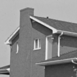
Figure 2: Aggregating low-rank tensors to images. The original image is on top left. The PSNR of images reconstructed from $rank$-$1$ to $rank$-$8$ tensors are $27.88$dB, $34.78$dB, $36.54$dB, $36.65$dB, $36.67$dB, $36.76$dB, $37.00$dB, and $37.09$dB respectively.

Under the assumption that the grouped patches have similar structure, $\mathcal{T}_{p}$ has a low-rank property, which ensures that $\mathcal{T}_{p}$ can be represented by a relatively low-rank tensor $\mathcal{L}_{p}$. This low-rank imposition shares the same spirit with the hard thresholding algorithm [1]. In Fig. 2, we impose low rankness on tensors with size $8\times 8\times 20$ generated from a clean image using the above approach, and then aggregate the tensors back to images. As can be seen, reconstructed images with low-rank tensors can accurately approximate the original image. The images aggregated from $rank$-$3$ to $rank$-$8$ tensors are highly similar (with PSNR merely increased by $0.55$ dB), which indicates that in this case $rank$-$3$ tensors are adequate to represent the original image.

3.2 Image Recovery via ADMM

With the reconstructed low-rank tensors $\mathcal{L}_{p}$, the following optimization problem is proposed for CS recovery:

$${\hat{\boldsymbol{x}}}=\arg\min_{\boldsymbol{x}}\|\boldsymbol{y}-\boldsymbol{\Phi}\boldsymbol{x}\|_{2}^{2}+\eta\sum_{p}\|\tilde{\mathcal{T}}_{p}\boldsymbol{x}-\mathcal{L}_{p}\|_{F}^{2},$$ (9)

where $\tilde{\mathcal{T}}_{p}\boldsymbol{x}=\mathcal{T}_{p}$ denotes the tensor formed for each reference patch $\boldsymbol{x}_{p}$ and $\eta$ is a regularization parameter. The closed-form solution for this quadratic optimization problem is

$$\boldsymbol{x}=(\boldsymbol{\Phi}^{H}\boldsymbol{\Phi}+\eta\sum_{p}\tilde{\mathcal{T}}_{p}^{\top}\tilde{\mathcal{T}}_{p})^{-1}(\boldsymbol{\Phi}^{H}\boldsymbol{y}+\eta\sum_{p}\tilde{\mathcal{T}}_{p}^{\top}\mathcal{L}_{p}),$$ (10)

where $H$ is the Hermitian transpose operation, $\sum_{p}\tilde{\mathcal{T}}_{p}^{\top}\mathcal{L}_{p}$ denotes the results of averaging all of the similar patches for each reference patch, and each entry of $\sum_{p}\tilde{\mathcal{T}}_{p}^{\top}\tilde{\mathcal{T}}_{p}$ corresponds to an image pixel location whose value is the number of overlapping patches that cover this pixel location. In (10), the matrix to be inverted can be large, for which conjugate gradient descent (CG) is usually applied [8]. We adopt ADMM to solve this problem, introducing auxiliary variable $\boldsymbol{z}$. Applying ADMM to (9), we obtain the global objective function

$$({\hat{\boldsymbol{x}}},{\hat{\boldsymbol{z}}})=\arg\min_{\boldsymbol{x},\boldsymbol{z}} \|\boldsymbol{y}-\boldsymbol{\Phi}\boldsymbol{x}\|_{2}^{2}+\beta\|\boldsymbol{x}-\boldsymbol{z}+\frac{{\boldsymbol{\mu}}}{2\beta}\|_{2}^{2}$$

$$+\eta\sum_{p}\|\tilde{\mathcal{T}}_{p}\boldsymbol{z}-\mathcal{L}_{p}\|_{F}^{2},$$ (11)

where ${\boldsymbol{\mu}}$ is the Lagrange multiplier, and $\beta>0$ is the penalty parameter. Instead of minimizing $\boldsymbol{x}$ and $\boldsymbol{z}$ simultaneously, ADMM decomposes the problem into two subproblems that minimizes w.r.t $\boldsymbol{x}$ and $\boldsymbol{z}$, respectively. More specifically, the optimization problem in (3.2) consists of the following iterations:

$$\boldsymbol{z}^{t+1} =\arg\min_{\boldsymbol{z}}\beta\|\boldsymbol{x}^{t}-\boldsymbol{z}+\frac{{\boldsymbol{\mu}}^{t}}{2\beta}\|_{2}^{2}+\eta\sum_{p}\|\tilde{\mathcal{T}}_{p}\boldsymbol{z}-\mathcal{L}_{i}\|_{F}^{2},$$ (12)

$$\boldsymbol{x}^{t+1} =\arg\min_{\boldsymbol{x}}\|\boldsymbol{y}-\boldsymbol{\Phi}\boldsymbol{x}\|_{2}^{2}+\beta\|\boldsymbol{x}-\boldsymbol{z}^{t+1}+\frac{{\boldsymbol{\mu}}^{t}}{2\beta}\|_{2}^{2},$$ (13)

$${\boldsymbol{\mu}}^{t+1} ={\boldsymbol{\mu}}^{t}+2\beta(\boldsymbol{x}^{t+1}-\boldsymbol{z}^{t+1}).$$ (14)

Both $\boldsymbol{x}$ and $\boldsymbol{z}$ admit closed-form solutions. For fixed $\boldsymbol{x}^{t}$ and ${\boldsymbol{\mu}}^{t}$,

$$\boldsymbol{z}^{t+1}=(\eta\sum_{p}\tilde{\mathcal{T}}_{p}^{\top}\tilde{\mathcal{T}}_{p}+\beta{\bf I})^{-1}(\beta\boldsymbol{x}^{t}+\frac{{\boldsymbol{\mu}}^{t}}{2}+\eta\sum_{p}\tilde{\mathcal{T}}_{p}^{\top}\mathcal{L}_{p}).$$ (15)

Then we use the updated $\boldsymbol{z}^{t+1}$ to update $\boldsymbol{x}$,

$$\boldsymbol{x}^{t+1}={{\bf U}}^{-1}(\boldsymbol{\Phi}^{H}\boldsymbol{y}+\beta\boldsymbol{z}^{t+1}-\frac{{\boldsymbol{\mu}}^{t}}{2}),$$ (16)

where ${{\bf U}}^{-1}=(\boldsymbol{\Phi}^{H}\boldsymbol{\Phi}+\beta{\bf I})^{-1}$.

Algorithm 2 CS via Low-Rank TFA

0:  The observation measurement $\boldsymbol{y}$. Initialization:

1:  Set parameters $\eta$, $\beta$, $\ell$, $m$, $n$, $k$, $I$, and $J$.

2:  Pretrain $\mathcal{C}_{\theta}$ for inverting matrix $\boldsymbol{\Phi}^{H}\boldsymbol{\Phi}+\beta{\bf I}$ using (18);

3:  Obtain an estimated image $\hat{\boldsymbol{x}}$ from observation $\boldsymbol{y}$ using a fast CS method;

4:  Divide $\hat{\boldsymbol{x}}$ into a set of overlapping patches;

5:  Initialize $\boldsymbol{x}^{(0)}=\hat{\boldsymbol{x}}$; Image Restoration:

6:  for $i=0,1,...,I-1$ do

7:     Divide $\boldsymbol{x}^{(i)}$ into a set of overlapping patches with size $m\times n$;

8:     Form a set of tensors with size $m\times n\times k$ using patch block matching;

9:     Decompose tensors using Jenrich’s Algorithm;

10:     Impose low rankness on tensors via (8) and generate a set of $rank$-$\ell$ tensors; ADMM:

11:     Initialize ${\boldsymbol{\mu}}^{0}=0$, $\boldsymbol{x}^{0}=\boldsymbol{x}^{(i)}$

12:     for $j=0,1,...,J-1$ do

13:        Update $\boldsymbol{z}^{j+1}$ via (15);

14:        if $\boldsymbol{\Phi}$ is a partial Fourier transform matrix then

15:           Update $\boldsymbol{x}^{j+1}$ via (21);

16:        else

17:           Update $\boldsymbol{x}^{j+1}$ via (19);

18:        end if

19:        Update ${\boldsymbol{\mu}}^{j+1}$ via (14);

20:     end for

21:     Update $\boldsymbol{x}^{(i+1)}=\boldsymbol{x}^{J}$

22:  end for

23:  Output: The reconstructed image $\hat{\boldsymbol{x}}=\boldsymbol{x}^{(I)}$.

3.2.1 Pretrained Deep Convolutional Architectures

In (16), the term ${{\bf U}}^{-1}$ involves an expensive matrix inversion, which makes direct computation of $\boldsymbol{x}^{t+1}$ impractical. An inversion-free approach proposed by [41] addresses this problem by learning a convolutional neural network to approximate the matrix inversion. Note that training this neural network is data-independent since ${{\bf U}}^{-1}$ is only dependent on $\boldsymbol{\Phi}$. Applying the Sherman-Morrison-Woodbury formula, we reduce this matrix inversion to a smaller scale,

$${{\bf U}}^{-1}=\beta^{-1}({\bf I}-\boldsymbol{\Phi}^{H}{{\bf V}}^{-1}\boldsymbol{\Phi}),$$ (17)

where ${{\bf V}}^{-1}=(\beta{\bf I}+\boldsymbol{\Phi}\boldsymbol{\Phi}^{H})^{-1}$ has the dimension $m\times m$. To approximate ${{\bf V}}^{-1}$, a trainable deep convolutional neural network $\mathcal{C}_{\theta}$ parameterized by $\theta$ is employed, i.e., $\mathcal{C}_{\theta}\approx{{\bf V}}^{-1}$. $\mathcal{C}_{\theta}$ is learned by minimizing the sum of two reconstruction losses of two auto-encoders with shared weights

$$\arg\min_{\theta}\mathbb{E}_{\epsilon}[\|\epsilon-\mathcal{C}_{\theta}{{\bf V}}\epsilon\|_{2}^{2}+\|\epsilon-{{\bf V}}\mathcal{C}_{\theta}\epsilon\|],$$ (18)

where ${{\bf V}}=\beta{\bf I}+\boldsymbol{\Phi}\boldsymbol{\Phi}^{H}$ can be computed directly, and $\epsilon$ is sampled from publicly available image datasets [10]. Note that $\mathcal{C}_{\theta}$ is pretrained for different $\boldsymbol{\Phi}$ and $\beta$. By plugging the learned $\mathcal{C}_{\theta}$ into (17), we obtain a reusable term ${{\bf U}}^{-1}=\beta^{-1}({\bf I}-\boldsymbol{\Phi}^{H}\mathcal{C}_{\theta}\boldsymbol{\Phi})$ as the replacement for the cumbersome inversion matrix. Hence $\boldsymbol{x}^{t+1}$ is updated by

$$\boldsymbol{x}^{t+1}=\beta^{-1}({\bf I}-\boldsymbol{\Phi}^{H}\mathcal{C}_{\theta}\boldsymbol{\Phi})(\boldsymbol{\Phi}^{H}\boldsymbol{y}+\beta\boldsymbol{z}^{t+1}-\frac{{\boldsymbol{\mu}}^{t}}{2}).$$ (19)

3.2.2 Fourier space solution

Equation (16) can be solved by transforming the problem from the image space into the Fourier space when $\boldsymbol{\Phi}$ is a partial Fourier transform matrix [11]. For a down-sampling matrix ${\bf D}$ and a Fourier transform matrix ${{\bf F}}$, $\boldsymbol{\Phi}={\bf D}{{\bf F}}$ is substituted into (16)

$$\boldsymbol{x}^{t+1}=({\bf D}^{H}{\bf D}+\beta{\bf I})^{-1}({{\bf F}}^{H}{\bf D}^{H}\boldsymbol{y}+(\beta\boldsymbol{z}^{t+1}-\frac{{\boldsymbol{\mu}}^{t}}{2})),$$ (20)

where the inverse matrix $({\bf D}^{H}{\bf D}+\beta{\bf I})^{-1}$ is a diagonal matrix and thus can be computed easily. Equation (20) is equivalent to

$$\boldsymbol{x}^{t+1}={{\bf F}}^{H}\{({\bf D}^{H}{\bf D}+\beta{\bf I})^{-1}({\bf D}^{H}\boldsymbol{y}+{{\bf F}}(\beta\boldsymbol{z}^{t+1}-\frac{{\boldsymbol{\mu}}^{t}}{2}))\}.$$ (21)

Therefore, $\boldsymbol{x}^{t+1}$ can be obtained by applying inverse Fourier transform to terms in the brackets of the right hand side of (21).

4 Experiments

Table 1: Reconstruction PSNR (dB) and SSIM of $8$ images using different CS recovery methods at different CSr.

Image	Method	CSr
		0.02	0.04	0.06	0.08	0.10
Barbara	BM3D-CS	16.44, 0.389	18.03, 0.422	19.70, 0.470	21.85, 0.561	23.70, 0.635
	TVAL3	21.32, 0.588	22.58, 0.620	23.28, 0.639	23.78, 0.654	24.25, 0.667
	NLR-CS	16.79, 0.400	18.90, 0.433	20.56, 0.501	24.00, 0.659	25.13, 0.725
	D-AMP	15.08, 0.354	17.76, 0.417	20.44, 0.496	22.66, 0.623	24.05, 0.660
	Ours	26.15, 0.812	27.29, 0.835	27.40, 0.837	28.05, 0.848	28.30, 0.852
Boats	BM3D-CS	16.76, 0.398	17.98, 0.440	20.11, 0.507	23.21, 0.624	24.65, 0.687
	TVAL3	21.58, 0.634	23.66, 0.681	24.57, 0.699	25.22, 0.713	25.75, 0.725
	NLR-CS	17.20, 0.409	19.41, 0.489	21.76, 0.559	23.76, 0.638	25.52, 0.711
	D-AMP	15.52, 0.365	18.41, 0.456	20.76, 0.528	22.85, 0.600	25.22, 0.703
	Ours	30.79, 0.898	31.73, 0.909	31.84, 0.910	32.35, 0.916	32.33, 0.912
Cameraman	BM3D-CS	16.84, 0.432	18.34, 0.496	20.62, 0.585	22.32, 0.654	23.85, 0.711
	TVAL3	20.33, 0.557	21.53, 0.579	22.02, 0.580	22.37, 0.578	23.19, 0.688
	NLR-CS	17.00, 0.436	19.10, 0.531	21.60, 0.620	23.99, 0.709	26.25, 0.789
	D-AMP	16.13, 0.401	17.51, 0.461	19.84, 0.562	21.74, 0.629	23.61, 0.705
	Ours	25.88, 0.828	26.47, 0.829	26.66, 0.823	27.16, 0.824	27.64, 0.819
Foreman	BM3D-CS	18.96, 0.610	21.06, 0.680	25.48, 0.726	29.80, 0.831	31.69, 0.866
	TVAL3	23.35, 0.777	26.81, 0.808	28.47, 0.821	29.45, 0.828	30.02, 0.833
	NLR-CS	19.64, 0.645	22.33, 0.695	28.09, 0.809	31.68, 0.865	34.15, 0.900
	D-AMP	19.42, 0.639	22.07, 0.687	26.31, 0.750	29.12, 0.813	31.90, 0.872
	Ours	34.01, 0.934	34.61, 0.936	35.18, 0.937	35.33, 0.939	36.02, 0.939
House	BM3D-CS	18.12, 0.518	20.35, 0.590	25.79, 0.755	29.78, 0.816	30.50, 0.824
	TVAL3	22.57, 0.706	24.58, 0.724	26.36, 0.740	27.63, 0.766	28.68, 0.814
	NLR-CS	18.80, 0.554	21.77, 0.620	27.16, 0.761	31.23, 0.835	33.66, 0.869
	D-AMP	17.74, 0.492	19.93, 0.577	24.00, 0.693	27.39, 0.758	29.84, 0.818
	Ours	30.42, 0.873	31.76, 0.884	33.07, 0.898	34.32, 0.910	34.80, 0.913
Lena	BM3D-CS	16.09, 0.427	18.22, 0.511	20.47, 0.603	23.55, 0.694	24.63, 0.729
	TVAL3	21.60, 0.671	23.23, 0.693	23.88, 0.697	24.41, 0.701	24.81, 0.705
	NLR-CS	16.71, 0.461	19.07, 0.545	21.36, 0.649	25.47, 0.746	25.82, 0.771
	D-AMP	15.53, 0.399	17.21, 0.485	19.93, 0.567	22.29, 0.681	24.60, 0.733
	Ours	28.51, 0.881	29.70, 0.894	29.85, 0.889	30.42, 0.898	30.65, 0.896
Monarch	BM3D-CS	14.55, 0.352	15.24, 0.390	17.65, 0.500	19.75, 0.581	21.64, 0.666
	TVAL3	17.31, 0.537	18.91, 0.577	19.82, 0.595	20.56, 0.611	21.24, 0.624
	NLR-CS	14.69, 0.357	16.03, 0.413	18.53, 0.552	21.84, 0.686	25.12, 0.796
	D-AMP	14.01, 0.334	14.86, 0.366	17.55, 0.497	19.84, 0.587	21.77, 0.675
	Ours	26.14, 0.884	27.28, 0.895	28.21, 0.901	28.97, 0.904	29.25, 0.904
Parrots	BM3D-CS	16.62, 0.506	19.32, 0.613	23.07 0.693	25.04, 0.761	26.10, 0.787
	TVAL3	21.11, 0.714	22.90, 0.722	23.47, 0.714	24.38, 0.770	25.84, 0.804
	NLR-CS	17.39, 0.550	20.84, 0.681	24.95, 0.782	28.18, 0.835	30.35, 0.875
	D-AMP	16.89, 0.520	19.55, 0.619	22.62, 0.684	24.10, 0.711	26.31, 0.792
	Ours	28.28, 0.899	28.88, 0.893	29.22, 0.890	29.55, 0.887	29.84, 0.885
Average	BM3D-CS	16.80, 0.454	18.57, 0.518	21.61, 0.605	24.42, 0.690	25.85, 0.738
	TVAL3	21.15, 0.648	23.02, 0.676	23.98, 0.685	24.72, 0.703	25.47, 0.732
	NLR-CS	17.28, 0.477	19.68, 0.551	23.00, 0.654	26.27, 0.747	28.25, 0.805
	D-AMP	16.29, 0.438	18.41, 0.509	21.43, 0.610	23.75, 0.675	25.91, 0.745
	Ours	28.77, 0.876	29.71, 0.884	30.18, 0.886	30.77, 0.891	31.10, 0.890

We conduct experiments on both noisy and noiseless CS mearurements of $8$ test images: Barbara, Boats, Cameraman, Foreman, House, Lena, Monarch, and Parrots. All images are resized to $256\times 256$. Since excellent results have been obtained when the CS rate is large, i.e. ${\rm CSr}>0.1$ [11, 29], we here focus on testing cases with limited number of measurements (${\rm CSr}<0.1$). The CS measurements are generated by pseudo-radial sampling of the test images in the Fourier domain. Unlike traditional random sampling schemes, pseudo-radial sampling produces streaking artifacts which are more difficult to remove. We also perform experiments using an $M\times N$ random sensing matrix generated by a standard Gaussian distribution. The deep convolutional architecture $C_{\theta}$ is pretrained by the sensing matrix then used in ADMM to solve the expensive matrix inversion. A DCT based CS recovery algorithm [52] is used for the initial image estimate. The main parameters of the proposed method are set as follows: patch size $4\times 4$, number of similar patches for each reference patch $50$, and the imposed low rank is $20$. The regularization parameter $\eta$ and the ADMM parameter $\beta$ are tuned separately for each sensing rate. In practice, we have found that ADMM converges fast after a few iterations and the performance gain is mainly from our low-rank TFA. Thus we set the number of outer-loop iterations to $I=50$ and the number of inner loop iterations $J=2$. Experimental results for noiseless CS measurements and noisy CS measurements are evaluated by peak signal-to-noise ratio (PSNR) and structural similarity (SSIM) [40].

(a)

(b)

(c)

(d)

Figure 3: Reconstruction results from noiseless CS measurements for Foreman at CSr$=0.02$. (a) Original image; (b) TVAL3 (23.35 dB); (c) NLR-CS (19.64 dB); (d) Ours (34.01 dB).

(a)

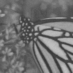
(b)

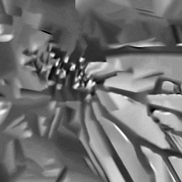
(c)

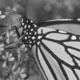
(d)

Figure 4: Reconstruction results from noiseless CS measurements for Monarch at CSr$=0.06$. (a) Original image; (b) TVAL3 (19.82 dB); (c) NLR-CS (18.51 dB); (d) Ours (28.21 dB).

4.1 Baselines

We compare our results with four competitive CS image restoration algorithms: BM3D-CS [15], TVAL3 [22], NLR-CS [11] and D-AMP [29]. BM3D-CS is a nonparametric method that applies block matching and 3D filtering algorithm [9] on compressive sensing. TVAL3 restores images by combining the classic augmented Lagrangian multiplier method with total-variation regularization. NLR-CS is currently a state-of-the-art method that uses a nonlocal low-rank regularization method along with ADMM to solve image CS problems. D-AMP employs a denoiser in an approximate message passing framework, achieving state-of-the-art performance on noisy measurements, especially at high CS rates. The source codes of these baseline methods are downloaded from the respective author’s website and parameters for these algorithms are set to their default values.

4.2 Experiments with Noiseless CS Measurements

We first perform CS image restoration experiments from noiseless measurements using pseudo-radial sampling scheme at five different CS rates, i.e., CSr = {$0.02$, $0.04$, $0.06$, $0.08$, $0.10$}. Table 1 summarizes the results of our proposed algorithm compared with various CS inversion algorithms at different CSr values. Both BM3D-CS and the state-of-the-art methods NLR-CS and D-AMP suffer at extremely low CSr. As CSr increases, NLR-CS yields significant performance improvements, which leads one of its results at higher CSr ($0.10$) to surpass other methods. Our proposed method achieves the best performance in all cases when CSr$<0.1$. On average, our proposed NLR-TFA algorithm outperforms all other competing methods at CSr = {$0.02$, $0.04$, $0.06$, $0.08$, and $0.10$}. The PSNR gains of our NLR-TFA over BM3D-CS, TVAL3, NLR-CS and D-AMP can be as much as $15.04$ dB, $10.65$ dB, $14.36$ dB, and $14.58$ dB, respectively. Furthermore, it can be observed that our average reconstruction PSNR only decreases by $2.33$ dB as CSr decreases from $0.10$ to $0.02$, while this number for NLR-CS and D-AMP are $10.67$ dB and $9.62$ dB, respectively, indicating that the proposed method is very stable at low CSr, i.e., with limited number of measurements.

To evaluate the reconstruction visually, two examples of restored Foreman and Monarch images at CSr of $0.02$ and $0.06$ are shown in Figs. 3 and 4. It is evident that our method recovers the best visual quality among all competiting methods. Large-scale sharp edges and small-scale fine structures are both reconstructed in two images. In particular, at extremely low CSr of $0.02$, our NLR-TFA method (Fig. 3(d)) can effectively approximate the original image while some other methods, such as NLR-CS, can only reconstruct scratches (Fig. 3(c)).

Table 2: PSNR(dB) of reconstructions from measurements generated by random Gaussian sampling of 8 images at different CSr.

Image	Method	CSr
		0.02	0.04	0.06	0.08
Barbara	D-AMP	15.79	17.56	19.20	21.96
	Ours	24.13	25.52	26.38	27.22
Boats	D-AMP	16.06	17.93	19.84	22.47
	Ours	26.04	27.44	28.59	29.51
Cameraman	D-AMP	16.66	18.32	19.79	22.42
	Ours	23.59	24.66	25.41	26.15
Foreman	D-AMP	20.50	22.78	25.75	28.40
	Ours	27.72	29.23	30.66	31.47
House	D-AMP	18.61	20.85	24.42	26.97
	Ours	26.68	28.20	29.48	30.17
Lena	D-AMP	16.34	18.15	19.77	22.15
	Ours	24.63	26.04	26.99	27.78
Monarch	D-AMP	14.50	15.68	17.94	19.93
	Ours	21.57	23.01	24.19	24.89
Parrots	D-AMP	17.49	19.38	22.56	25.24
	Ours	25.92	27.19	27.96	28.54
Average	D-AMP	16.99	18.83	21.15	23.69
	Ours	25.04	26.41	27.46	28.22

We next generate CS measurements by sampling the test images with a random Gaussian sensing matrix. A deep convolutional neural network $\mathcal{C}_{\theta}$ is pretrained using the sensing matrix to solve the large-scale matrix inversion problem in ADMM. We compare our results with D-AMP which provides random Gaussian sensing implementations in their sourcing code. The reconstruction results at CSr of $0.02$, $0.04$, $0.06$ and $0.08$ are shown in Table 2. Our proposed method outperforms D-AMP on all test images and sensing rates. In addition, the runtime of the algorithm using this inversion-free approach is also much faster than using approaches with inner-loop updates, such as conjugate gradient (CG). This demonstrates the efficiency and accuracy of the deep convolutional architecture on approximating the inversion matrix.

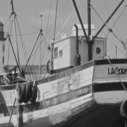
(a)

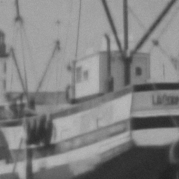
(b)

(c)

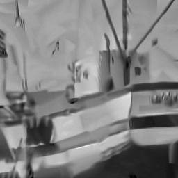
(d)

(e)

Figure 5: Reconstruction results of Boats images from noisy CS measurements with noise standard deviation equal to $30$ at CSr$=0.10$. (a) Original image; (b) TVAL3 (24.02 dB); (c) NLR-CS (23.48 dB); (d) DAMP (24.71 dB); (e) Ours (30.97 dB).

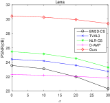
(a)

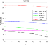
(b)

Figure 6: Comparison of different CS methods with noisy measurements for Lena and Parrots images. (a) CSr$=0.08$. (b) CSr=$0.04$.

Table 3: PSNR(dB) of reconstructions with variant patch sizes at different CSr for foreman image.

Patch Size	CSr
	0.02	0.04	0.06	0.08	0.10
$4\times 4$	34.01	34.61	35.18	35.33	36.02
$6\times 6$	31.16	31.95	32.72	32.88	33.59
$8\times 8$	29.63	30.41	31.37	31.68	32.24
$10\times 10$	28.57	29.45	30.44	30.86	31.33
$12\times 12$	27.39	28.61	29.60	30.11	30.54

Patch Size Selection

We have conducted experiments using different patch sizes. As can be seen from Table 3 (in the pseudo-radial sampling scheme), smaller patch sizes lead to better reconstruction results. When we adopt patch size of $4\times 4$ on the foreman image, the PSNR is significantly increased compared to results with larger patch sizes. Similar conclusions are found on other images as well. In addition, the running time of our model is largely influenced by the tensor size. For tensor size of $4\times 4\times 50$ (image patch size $4\times 4$ and $50$ similar patches for each reference patch), the average running time at CSr=$0.06$ is about 10 minutes on a desktop with i7 CPU @3.4GHz and 24G RAM.

4.3 Experiments with Noisy CS Measurements

Similar experiments are conducted with noisy CS measurements to show the robustness of our algorithm to noise. The noisy CS measurements are obtained by adding random zero-mean Gaussian noise to the noiseless CS measurements. We test the algorithms at three levels of noise, with standard deviation $\sigma$={$10$, $20$, $30$}. The PSNR comparison of all methods for Boats and Monarch images at sensing rates of $0.10$ and $0.04$, respectively, are shown in Fig. 6. Our proposed NLR-TFA outperforms other competing methods at all levels of noise. Furthermore, D-AMP shows great robustness to noise while BM3D-CS and NLR-CS are relatively sensitive to high-level noise. As the noise level increases, the reconstruction performance of our algorithm decreases slowly. This shows that the proposed method is robust to noise. In Fig. 5, we show the reconstructions of Boats images using various algorithms at CSr=$0.10$ and $\sigma=30$. The proposed NLR-TFA clearly yields the best reconstruction and is robust to noise.

5 Conclusion

We have presented a low-rank tensor-factor-analysis-based approach to solve image-restoration problems. A tensor is generated by concatenating similar patches from the estimated image for each exemplar patch. Low-rank is imposed on the tensors to exploit non-local correlation and the high-order structure information via tensor factorization. ADMM is employed on low-rank tensors, where we use either a pretrained convolutional architecture or Fourier approaches to solve a matrix inversion. Experimental results demonstrate that the proposed NLR-TFA method outperforms state-of-the-art algorithms on CS image reconstruction at low CS sampling rates.

We have demonstrated the superiority of our model in image CS with three-way tensors, which can also be used in depth CS [25, 26, 53], polarization CS  [39] and dynamic range CS [48]. Future work includes extending the model to four-way tensors for video CS [24, 27, 35, 36, 45, 46, 54, 55, 56, 60, 61], hyperspectral image CS [7, 62] and to five-way tensors for joint spectral-temporal CS [37, 38].

References

- [1] T. Blumensath and M. E. Davies. Iterative hard thresholding for compressed sensing. Applied and Computational Harmonic Analysis, 27(3):265 – 274, 2009.
- [2] S. Boyd, N. Parikh, E. Chu, B. Peleato, and J. Eckstein. Distributed optimization and statistical learning via the alternating direction method of multipliers. Foundations and Trends® in Machine Learning, 3(1):1–122, 2011.
- [3] A. Buades, B. Coll, and J.-M. Morel. A non-local algorithm for image denoising. In Computer Vision and Pattern Recognition, 2005. CVPR 2005. IEEE Computer Society Conference on, volume 2, pages 60–65. IEEE, 2005.
- [4] A. Buades, J.-L. Lisani, and M. Miladinović. Patch-based video denoising with optical flow estimation. IEEE Transactions on Image Processing, 25(6):2573–2586, 2016.
- [5] E. J. Candès, J. Romberg, and T. Tao. Robust uncertainty principles: Exact signal reconstruction from highly incomplete frequency information. IEEE Transactions on information theory, 52(2):489–509, 2006.
- [6] E. J. Candes and T. Tao. Decoding by linear programming. IEEE transactions on information theory, 51(12):4203–4215, 2005.
- [7] X. Cao, T. Yue, X. Lin, S. Lin, X. Yuan, Q. Dai, L. Carin, and D. J. Brady. Computational snapshot multispectral cameras: Toward dynamic capture of the spectral world. IEEE Signal Processing Magazine, 33(5):95–108, Sept 2016.
- [8] J. Chang, C.-L. Li, B. Póczos, B. Kumar, and A. C. Sankaranarayanan. One network to solve them all—solving linear inverse problems using deep projection models. arXiv preprint arXiv:1703.09912, 2017.
- [9] K. Dabov, A. Foi, V. Katkovnik, and K. Egiazarian. Image denoising by sparse 3-d transform-domain collaborative filtering. IEEE Transactions on image processing, 16(8):2080–2095, 2007.
- [10] J. Deng, W. Dong, R. Socher, L.-J. Li, K. Li, and L. Fei-Fei. ImageNet: A Large-Scale Hierarchical Image Database. In CVPR09, 2009.
- [11] W. Dong, G. Shi, X. Li, Y. Ma, and F. Huang. Compressive sensing via nonlocal low-rank regularization. IEEE Transactions on Image Processing, 23(8):3618–3632, 2014.
- [12] D. L. Donoho. Compressed sensing. IEEE Trans. Inf. Theor., 52(4):1289–1306, Apr. 2006.
- [13] D. L. Donoho. Compressed sensing. IEEE Transactions on information theory, 52(4):1289–1306, 2006.
- [14] M. F. Duarte, M. A. Davenport, D. Takhar, J. N. Laska, T. Sun, K. F. Kelly, and R. G. Baraniuk. Single-pixel imaging via compressive sampling. IEEE Signal Processing Magazine, 25(2):83–91, March 2008.
- [15] K. Egiazarian, A. Foi, and V. Katkovnik. Compressed sensing image reconstruction via recursive spatially adaptive filtering. In Image Processing, 2007. ICIP 2007. IEEE International Conference on, volume 1, pages I–549. IEEE, 2007.
- [16] M. Elad and M. Aharon. Image denoising via sparse and redundant representations over learned dictionaries. IEEE Transactions on Image processing, 15(12):3736–3745, 2006.
- [17] S. Gu, L. Zhang, W. Zuo, and X. Feng. Weighted nuclear norm minimization with application to image denoising. In Proceedings of the IEEE Conference on Computer Vision and Pattern Recognition, pages 2862–2869, 2014.
- [18] L. He and L. Carin. Exploiting structure in wavelet-based bayesian compressive sensing. IEEE Transactions on Signal Processing, 57(9):3488–3497, September 2009.
- [19] T. G. Kolda and B. W. Bader. Tensor decompositions and applications. SIAM Rev., 51(3):455–500, Aug. 2009.
- [20] K. Kulkarni, S. Lohit, P. Turaga, R. Kerviche, and A. Ashok. Reconnet: Non-iterative reconstruction of images from compressively sensed measurements. In The IEEE Conference on Computer Vision and Pattern Recognition (CVPR), June 2016.
- [21] S. Leurgans, R. Ross, and R. Abel. A decomposition for three-way arrays. SIAM Journal on Matrix Analysis and Applications, 14(4):1064–1083, 1993.
- [22] C. Li, W. Yin, H. Jiang, and Y. Zhang. An efficient augmented lagrangian method with applications to total variation minimization. Computational Optimization and Applications, 56(3):507–530, 2013.
- [23] Z. Lin, M. Chen, and Y. Ma. The augmented lagrange multiplier method for exact recovery of corrupted low-rank matrices. arXiv preprint arXiv:1009.5055, 2010.
- [24] P. Llull, X. Liao, X. Yuan, J. Yang, D. Kittle, L. Carin, G. Sapiro, and D. J. Brady. Coded aperture compressive temporal imaging. Optics Express, 21(9):10526–10545, 2013.
- [25] P. Llull, X. Yuan, L. Carin, and D. Brady. Image translation for single-shot focal tomography. Optica, 2(9):822–825, 2015.
- [26] P. Llull, X. Yuan, X. Liao, J. Yang, L. Carin, G. Sapiro, and D. Brady. Compressive extended depth of field using image space coding. In Computational Optical Sensing and Imaging (COSI), pages 1–3, 2014.
- [27] P. Llull, X. Yuan, X. Liao, J. Yang, D. Kittle, L. Carin, G. Sapiro, and D. J. Brady. Compressed Sensing and its Applications: MATHEON Workshop 2013, chapter Temporal Compressive Sensing for Video, pages 41–74. Springer International Publishing, 2015.
- [28] M. Lustig, D. L. Donoho, J. M. Santos, and J. M. Pauly. Compressed sensing mri. IEEE Signal Processing Magazine.
- [29] C. A. Metzler, A. Maleki, and R. G. Baraniuk. From denoising to compressed sensing. IEEE Transactions on Information Theory, 62(9):5117–5144, Sept 2016.
- [30] A. Mousavi, A. B. Patel, and R. G. Baraniuk. A deep learning approach to structured signal recovery. In Communication, Control, and Computing (Allerton), 2015 53rd Annual Allerton Conference on, pages 1336–1343. IEEE, 2015.
- [31] F. Nie, H. Huang, and C. H. Ding. Low-rank matrix recovery via efficient schatten -norm minimization. In AAAI, 2012.
- [32] Y. Peng, D. Meng, Z. Xu, C. Gao, Y. Yang, and B. Zhang. Decomposable nonlocal tensor dictionary learning for multispectral image denoising. In Proceedings of the IEEE Conference on Computer Vision and Pattern Recognition, pages 2949–2956, 2014.
- [33] P. Rai, Y. Wang, S. Guo, G. Chen, D. Dunson, and L. Carin. Scalable bayesian low-rank decomposition of incomplete multiway tensors. In Proceedings of the 31st International Conference on Machine Learning, volume 32, pages 1800–1808, 2014.
- [34] N. D. Sidiropoulos, L. De Lathauwer, X. Fu, K. Huang, E. E. Papalexakis, and C. Faloutsos. Tensor decomposition for signal processing and machine learning. IEEE Transactions on Signal Processing, 65(13):3551–3582, 2017.
- [35] Y. Sun, X. Yuan, and S. Pang. High-speed compressive range imaging based on active illumination. Opt. Express, 24(20):22836–22846, Oct 2016.
- [36] Y. Sun, X. Yuan, and S. Pang. Compressive high-speed stereo imaging. Opt. Express, 25(15):18182–18190, July 2017.
- [37] T. Tsai, P. Llull, X. Yuan, L. Carin, and D. Brady. Coded aperture compressive spectral-temporal imaging. In Computational Optical Sensing and Imaging (COSI), pages 1–3, 2015.
- [38] T.-H. Tsai, P. Llull, X. Yuan, D. J. Brady, and L. Carin. Spectral-temporal compressive imaging. Optics Letters, 40(17):4054–4057, Sep 2015.
- [39] T.-H. Tsai, X. Yuan, and D. J. Brady. Spatial light modulator based color polarization imaging. Optics Express, 23(9):11912–11926, May 2015.
- [40] Z. Wang, A. C. Bovik, H. R. Sheikh, and E. P. Simoncelli. Image quality assessment: From error visibility to structural similarity. Trans. Img. Proc., 13(4):600–612, Apr. 2004.
- [41] Q. Wei, K. Fan, L. Carin, and K. A. Heller. An inner-loop free solution to inverse problems using deep neural networks. arXiv preprint arXiv:1709.01841, 2017.
- [42] B. Wen, Y. Li, L. Pfister, and Y. Bresler. Joint adaptive sparsity and low-rankness on the fly: an online tensor reconstruction scheme for video denoising. In IEEE International Conference on Computer Vision (ICCV), 2017.
- [43] Q. Xie, Q. Zhao, D. Meng, Z. Xu, S. Gu, W. Zuo, and L. Zhang. Multispectral images denoising by intrinsic tensor sparsity regularization. In The IEEE Conference on Computer Vision and Pattern Recognition (CVPR), June 2016.
- [44] Y. Xie, S. Gu, Y. Liu, W. Zuo, W. Zhang, and L. Zhang. Weighted schatten -norm minimization for image denoising and background subtraction. IEEE transactions on image processing, 25(10):4842–4857, 2016.
- [45] J. Yang, X. Liao, X. Yuan, P. Llull, D. J. Brady, G. Sapiro, and L. Carin. Compressive sensing by learning a Gaussian mixture model from measurements. IEEE Transaction on Image Processing, 24(1):106–119, January 2015.
- [46] J. Yang, X. Yuan, X. Liao, P. Llull, G. Sapiro, D. J. Brady, and L. Carin. Video compressive sensing using Gaussian mixture models. IEEE Transaction on Image Processing, 23(11):4863–4878, November 2014.
- [47] Y. Yang, J. Sun, H. Li, and Z. Xu. Deep admm-net for compressive sensing mri. In D. D. Lee, M. Sugiyama, U. V. Luxburg, I. Guyon, and R. Garnett, editors, Advances in Neural Information Processing Systems 29, pages 10–18. Curran Associates, Inc., 2016.
- [48] X. Yuan. Compressive dynamic range imaging via Bayesian shrinkage dictionary learning. Optical Engineering, 55(12):123110, 2016.
- [49] X. Yuan. Generalized alternating projection based total variation minimization for compressive sensing. In 2016 IEEE International Conference on Image Processing (ICIP), pages 2539–2543, Sept 2016.
- [50] X. Yuan, G. Huang, H. Jiang, and P. A. Wilford. Block-wise lensless compressive camera. In 2017 IEEE International Conference on Image Processing (ICIP), pages 31–35, Sept 2017.
- [51] X. Yuan, H. Jiang, G. Huang, and P. Wilford. Lensless compressive imaging. arXiv:1508.03498, 2015.
- [52] X. Yuan, H. Jiang, G. Huang, and P. Wilford. SLOPE: Shrinkage of local overlapping patches estimator for lensless compressive imaging. IEEE Sensors Journal, 16(22):8091–8102, November 2016.
- [53] X. Yuan, X. Liao, P. Llull, D. Brady, and L. Carin. Efficient patch-based approach for compressive depth imaging. Applied Optics, 55(27):7556–7564, Sep 2016.
- [54] X. Yuan, P. Llull, X. Liao, J. Yang, D. J. Brady, G. Sapiro, and L. Carin. Low-cost compressive sensing for color video and depth. In IEEE Conference on Computer Vision and Pattern Recognition (CVPR), pages 3318–3325, 2014.
- [55] X. Yuan and S. Pang. Compressive video microscope via structured illumination. In 2016 IEEE International Conference on Image Processing (ICIP), pages 1589–1593, Sept 2016.
- [56] X. Yuan and S. Pang. Structured illumination temporal compressive microscopy. Biomedical Optics Express, 7:746–758, 2016.
- [57] X. Yuan and Y. Pu. Convolutional factor analysis inspired compressive sensing. In 2017 IEEE International Conference on Image Processing (ICIP), pages 550–554, Sept 2017.
- [58] X. Yuan and Y. Pu. Parallel lensless compressive imaging via deep convolutional neural networks. Optics Express, 26(2):1962–1977, Jan 2018.
- [59] X. Yuan, V. Rao, S. Han, and L. Carin. Hierarchical infinite divisibility for multiscale shrinkage. IEEE Transactions on Signal Processing, 62(17):4363–4374, Sep. 1 2014.
- [60] X. Yuan, Y. Sun, and S. Pang. Compressive video microscope via structured illumination. In Computational Optical Sensing and Imaging (COSI), 2016.
- [61] X. Yuan, Y. Sun, and S. Pang. Compressive temporal rgb-d imaging. In Imaging and Applied Optics 2017 (3D, AIO, COSI, IS, MATH, pcAOP), page CTh1B.3. Optical Society of America, 2017.
- [62] X. Yuan, T.-H. Tsai, R. Zhu, P. Llull, D. J. Brady, and L. Carin. Compressive hyperspectral imaging with side information. IEEE Journal of Selected Topics in Signal Processing, 9(6):964–976, September 2015.
- [63] M. Zhou, H. Chen, L. Ren, G. Sapiro, L. Carin, and J. W. Paisley. Non-parametric bayesian dictionary learning for sparse image representations. In Advances in neural information processing systems, pages 2295–2303, 2009.