Adaptive Decision Making via Entropy Minimization

Abstract

An agent choosing between various actions tends to take the one with the lowest cost. But this choice is arguably too rigid (not adaptive) to be useful in complex situations, e.g., where exploration-exploitation trade-off is relevant in creative task solving or when stated preferences differ from revealed ones. Here we study an agent who is willing to sacrifice a fixed amount of expected utility for adaptation. How can/ought our agent choose an optimal (in a technical sense) mixed action? We explore consequences of making this choice via entropy minimization, which is argued to be a specific example of risk-aversion. This recovers the $\epsilon$-greedy probabilities known in reinforcement learning. We show that the entropy minimization leads to rudimentary forms of intelligent behavior: (i) the agent assigns a non-negligible probability to costly events; but (ii) chooses with a sizable probability the action related to less cost (lesser of two evils) when confronted with two actions with comparable costs; (iii) the agent is subject to effects similar to cognitive dissonance and frustration. Neither of these features are shown by entropy maximization.

I Introduction

Consider an agent who has to choose between a number of different actions ${\cal A}_{1},...,{\cal A}_{n}$. Before taking action, consequences of each action ${\cal A}_{k}$ are subjectively estimated to have the cost $\varepsilon_{k}$ (or the utility $u_{k}=-\varepsilon_{k}$). The basic tenet of decision theory is that the agent ought to choose the action that minimizes the cost (or maximizes the utility) luce . In terms of probabilities $p_{k}$ for various actions ($p_{k}\geq 0$, $\sum_{k=1}^{n}p_{k}=1$), this amounts to taking the action $\ell$ related to the least cost (if it exists and is available):

$$p_{\ell}=1,\qquad p_{k\not=\ell}=0,\qquad\varepsilon_{\ell}<\varepsilon_{k\not=\ell},\qquad k=1,...,n.$$ (1)

There are, however, situations where $\varepsilon_{k}$ may change after actions are taken, also as a result of those actions . Here is an example that points against choosing (1), and illustrates our problem. You got 100 eggs and several baskets, which seem to have different durabilities (i.e. utilities). The probability with which an action, i.e. a basket, is taken refers to the fraction of eggs in it. Even if the most durable basket may appear to support all the eggs, it is not wise to put everything in one basket. First the durability of a basket can change due to very eggs inside of it. Second, the durability can change unexpectedly due to hindrances. Third, you loose the possibility to explore other baskets that may turn out to be more durable than you thought. Let us now mention several more, broadly defined situations, where “putting all eggs into one basket” is not good.

– In reinforcement learning the preliminary costs $\varepsilon_{k}$ do change due to the actions taken barto . Even if these changes are assumed to be predictable, the agent still needs to make several actions before enough experience is accumulated.

– The exploration-exploitation dilemma is known in adaptive (biological, organizational, social) systems; see exp_exp ; exp_exp_1 for reviews. Exploring possibilities that seem inferior from a local viewpoint may provide advantages in the long run. Exploitation (in the narrow sense) makes the choice that does seem optimal at the moment of choice. Broader exploitation scenarios do account for adaptivity, but still concentrate on the most useful possibilities exp_exp_1 .

– In creative problem solving there are conceptually simple tasks which are nevertheless not easy to solve in practice because solving them via the least cost (implied by the statement of the problem and/or the previous experience of the solver) is a dead end handbook ; maier ; luchins . This Einstellung effect is one of the main hindrances of human creativity handbook ; maier ; luchins . Creative tasks can be solved only if (subjectively) less probable ways are looked at handbook ; maier .

How to assign prior probabilities to avoid the strictly deterministic (1)? Such probabilities should hold a natural constraint that actions related to higher cost are getting smaller probabilities. Two ad hoc solutions are especially simple: one can take into account only the second-best action, or take all non-best actions with the same (small) probability. In reinforcement learning the latter prior probability is known as the $\epsilon$-greedy barto . It is preferable to have a regular method of choosing non-deterministic probabilities, which will reflect people’s attitudes towards the decision making in an uncertain situation, and which will include the above ad hoc solutions as particular cases.

Here we explore the possibility of defining the prior probabilities via risk minimization (or maximization); see lola ; lopes for reviews on the notion of risk and its various interpretations. We assume that the agent first decides how much average utility $E-{\rm min}_{k}[\varepsilon_{k}]$ he invests into exploration by going into nonoptimal—in the sense of not holding (1)—behavior. We employ the notion of risk in a specific context, namely when comparing the behavior of agents having the same utilities for various actions and the same value of $E$. We argue below that maximizing (minimizing) risk in this specific situation can be done via maximizing (minimizing) the entropy $-\sum_{k=1}^{n}p_{k}\ln p_{k}$. People demonstrate both risk minimization (aversion) and maximization (seeking) tver ; baron , though the risk in those situations is a less specific (and more difficult to describe) notion—first because it involves agents having different utilities for same actions, and second because it involves a difference between the monetary value (gain or loss) and its utility.

Our results show that there are important behavioral differences between entropy-minimizing and entropy-maximizing agents. They are seen for at least three different actions (and the same $E$). The entropy-minimizing agent implements risk-aversion by weighting the least-cost action more, but he also assigns a non-negligible probability for the high-cost action—whereas the entropy-maximizing agent ignores it. The extent to which the high-cost action is accounted for by the entropy-minimizing agent depends on the amount of utility invested into exploration: investing more utility leads to assigning less probability. As we argue below, this closely relates with the notion of cognitive dissonance disso ; aronson . Another feature is frustration: due to competing local minima of entropy, the entropy-minimizing agent can abruptly change the action probabilities as a result of a small change of $E$. Also, when confronted with two actions with different, but comparable costs, the entropy-minimizing agent tends to select the one with a smaller cost (chooses the lesser of two evils), while the entropy-maximizing agent simply does not distinguish between them. The important point is that for a risk-minimizing agent (which does a constrained minimization of a concave function in a convex domain) choosing the probabilities of actions means selecting between several local minima. In contrast, the risk-seeking agent always has a unique and well-defined probabilistic solution that results from minimizing a convex function rock . We relate the above features of the entropy-minimizing agent with a rudimentary form of intelligence (see Section VII).

The remainder of this paper is organized as follows. Section II explains the statement of our problem. Section III discusses stochastic dominance, risk, majorization and its relation with entropy. In particular, Section III.4 provides general remarks and references on entropy optimization. The reader who agrees from the outset with entropy as a measure of risk (and uncertainty) can consult Sections II and III very briefly. The next two sections, IV and V, present details of (resp.) entropy minimization and maximization. The latter may seem to be standard, but Section V still contains salient points that are frequently overlooked. Section VI compares entropy maximization and minimization scenarios from the viewpoint of the agent’s behavior. We summarize in Section VII.

II Statement of the problem

II.1 Costs and constraints

Let us explain the above problem. An agent faces different actions $\{{\cal A}_{k}\}_{k=1}^{n}$ with (resp.) costs $\{\varepsilon_{k}\}_{k=1}^{n}$. These costs are subjective estimates of future consequences of actions made by the agent before deciding on those actions. After taking several actions, the agent can change his estimates also as a result of the actions taken. However, before taking actions he does not know in which specific way the costs will change. In such an agnostic situation, the agent faces two normative demands—he should behave according to $\{\varepsilon_{k}\}_{k=1}^{n}$, but he also should also explore all actions. Hence he decides to act via probabilities and implements two constraints. First, he decides to invest in the exploration of the average utility $E-{\rm min}_{k}[\varepsilon_{k}]$, where

$$E\equiv\sum_{k=1}^{n}p_{k}\,\varepsilon_{k},\qquad p_{k}\geq 0,\qquad\sum_{k=1}^{n}p_{k}=1,$$ (2)

and where $p_{k}$ are probabilities to be chosen. Within this formulation of the problem, we can regard $E$ to be under control of the agent.

Second, actions related to a lesser cost get higher probability:

$$(p_{k}-p_{l})(\varepsilon_{k}-\varepsilon_{l})\leq 0.$$ (3)

Recall that costs are negative utilities. We work with costs, since this makes explicit the analogy with statistical physics, where the cost corresponds to energy, and the natural tendency is to minimize the energy.

We order the costs and probabilities as

$$\varepsilon_{1}<\varepsilon_{2}<....<\varepsilon_{n},$$ (4)

$$p_{1}\geq p_{2}\geq...\geq p_{n}.$$ (5)

Note that the inequalities in (4) between costs are strict, since within the present study coinciding costs mean coinciding actions. Hence once the actions are different, so should be the costs. The reason for insisting on non-equal costs in (4) will be seen below.

II.2 Stated versus revealed preferences

We can look at this problem from a different angle. In human decision-making, it is known that preferences with respect to different actions can be determined in laboratory conditions (e.g., via surveys). This then defines their costs (negative utilities) (4). However, in reality (e.g., in complex conditions of a market) people generally do not strictly follow these preferences due to lack of cognitive abilities, insufficient attention, lack of a decision time, the need of an exploration behavior etc.. The difference between experimental and real-world choices is known as the problem of stated versus revealed preferences; see marley for a recent review. It is assumed in the psychology of choice that such cases can be described by assigning probabilities to each costs marley . Now, the above formulation does correspond to this situation, where (5) is a natural constraint on probabilities, and where $E-{\rm min}_{k}[\varepsilon_{k}]>0$ is not simply chosen by the agent, but is also due to objective problems described above. For $E-{\rm min}_{k}[\varepsilon_{k}]\to 0$, the agent is back to choosing the least-cost solution only.

II.3 Differences with respect to other models of decision theory

Above we described an agent who is uncertain about future consequences of his actions. Decision theory has models for that situation. The classic model (by Savage and others) luce ; jeffrey ; baron assumes that at the moment of action-taking there is an uncertain state of nature (environment) ${\cal S}_{\alpha}$ to be realized from $\{{\cal S}_{\alpha}\}_{\alpha=1}^{m}$ with probabilities $\{\pi_{\alpha}\}_{\alpha=1}^{m}$, which can be the agent’s subjective degrees of belief. These are called states of nature, since their future realization is independent from the action taken, but an action ${\cal A}_{i}$ in a state ${\cal S}_{\alpha}$ leads to consequences with costs $c_{i\alpha}$ luce ; jeffrey ; baron . The agent does know $\{\pi_{\alpha}\}_{\alpha=1}^{m}$ and $\{c_{i\alpha}\}_{i=1\,\alpha=1}^{n\quad m}$. Now one criterion for looking for the best action is to choose $i$ such that the expected cost $\sum_{\alpha=1}^{m}\pi_{\alpha}c_{i\alpha}$ is minimized over $i$ (i.e., the expected utility is maximized) luce ; jeffrey ; baron .

The classic model has limitations—e.g., that environmental states $\{{\cal S}_{\alpha}\}_{\alpha=1}^{m}$ are realized independently from actions. There are many cases where this simplistic assumption does not hold. Causal decision theory giba ; joyce ; skyrms ; rati ; shafer attempts to remedy this problem, but creates its own issues—e.g., replacing $\pi_{\alpha}$ by the conditional probability $\pi_{\alpha|i}$ of the state ${\cal S}_{\alpha}$ given the action ${\cal A}_{i}$ leads to paradoxical (if not unacceptable) conclusions nicknamed “voodoo” decisions skyrms . In response, the expected utility principle was changed to the concept of ratifiability jeffrey ; rati , but this proposal has its own problems rati , e.g.. it demands an unusual environment. Another response was to change the conditional probability $\pi_{\alpha|i}$ to the probability of conditional $\pi_{\alpha\Leftarrow i}$, which, in contrast to $\pi_{\alpha|i}$, is supposed to describe the causal influence of the action ${\cal A}_{i}$ on ${\cal S}_{\alpha}$ joyce ; giba . But $\pi_{\alpha\Leftarrow i}$ does not have a general definition giba , while some of its particular definitions are flawed shafer . Recent reviews show that all non-classical models of causal decision theory are problematic in one way or another rati ; giba ; shafer .

Our statement of the problem refers to an agnostic agent that (as yet) does not know about possible consequences of his actions in a complex and uncertain world. Even if he is going to learn about them, he still needs to perform several actions with certain prior probabilities. We do not assume any specific mechanism by which uncertain states of the world are realized and changed in response to actions. Hence, our model can be at best descriptional, but it starts from two normative demands: behave according to your own estimated costs (4) and explore all actions.

III Risk and entropy

III.1 Stochastic dominance, risk and majorization

Together with probabilities $p_{1},...,p_{n}$ in (2–5), we define another candidate probability with the same costs (4) and holding the same constraints (2, 3) with the same value of $E$:

$$q_{1}\geq q_{2}\geq...\geq q_{n}\geq 0,\quad\sum_{k=1}^{n}q_{k}=1,\quad E=\sum_{k=1}^{n}q_{k}\,\varepsilon_{k}.$$ (6)

We ask for criteria that should make $\{p_{k}\}^{n}_{k=1}$ more preferable than $\{q_{k}\}^{n}_{k=1}$. The well-known criterion of choosing for a smaller average cost obviously does not apply here. However, one can ask whether $\{p_{k}\}^{n}_{k=1}$ is less risky than $\{q_{k}\}^{n}_{k=1}$.

We emphasize that risk is generally a complex notion that raises conceptual and practical (resp. normative and descriptional) issues; see lola ; lopes ; pope ; baron ; aumann ; leshno ; tver ; chisar ; ahmad ; chin1 ; chin2 ; ng for reviews from various viewpoints. Our application of risk will be to a large extent free of those issues. There are two reasons for this. First, we do not focus on the difference between the commodity and its utility (cost); hence we are not concerned with the problem of convex/concave utility functions baron ; tver . Second, we always compare between lotteries (i.e., probabilities and their outcome costs) that are ordered in the same way [cf. (6, 5)] and refer to the same costs (4). Then a stringent definition of risk goes via the stochastic dominance condition; see luce ; haim for reviews. A risk-averse agent can start with the largest possible cost $\varepsilon_{n}$ and asks for its $p$-probability $p_{n}$ to be not larger than the $q$-probability $q_{n}$. Next, the $p$-probability $p_{n}+p_{n-1}$ of the cost to be larger or equal to $\varepsilon_{n-1}$ is compared with the corresponding $q$-probability $q_{n}+q_{n-1}$ etc. We end up with $n-1$ conditions $\sum_{i=n}^{k}p_{i}\leq\sum_{i=n}^{k}q_{i}$, or

$$\sum_{i=1}^{k}p_{i}\geq\sum_{i=1}^{k}q_{i},\qquad k=1,...,n-1,$$ (7)

so that if one of them holds strictly, then $\{p_{k}\}^{n}_{k=1}$ is less risky than $\{q_{k}\}^{n}_{k=1}$. We emphasize that the same $n-1$ conditions (7) emerge with an alternative definition of risk, when the agent maximizes the probability of the best outcome $\varepsilon_{1}$ etc. So within the present definition it does not matter whether a risk-averse agent selects for higher probabilities of lower-cost options, or for lower probabilities of higher-cost actions.

Due to (4, 5, 6), the stochastic dominance condition (7) coincides with the majorization condition major .

$$\{p_{k}\}_{k=1}^{n}\succ\{q_{k}\}_{k=1}^{n}.$$ (8)

In particular, for any $\{p_{k}\}_{k=1}^{n}$ we get $\{p_{k}\}_{k=1}^{n}\succ\{q_{k}=\frac{1}{n}\}_{k=1}^{n}$ (once $q_{k}$ holds the first condition in (6)), while $(1,0,..,0)\succ\{p_{k}\}_{k=1}^{n}$. Thus, in the present situation we have a natural correspondence between risk and majorization.

III.2 Measure of risk and Schur-concave functions

According to (7), we have $n-1$ different conditions; i.e., it is not a single number as a measure for risk. Hence even if (7) holds, i.e., $\{q_{k}\}_{k=1}^{n}$ is more risky that $\{p_{k}\}_{k=1}^{n}$, we do not have any obvious way of quantifying this relation via a single number or determine its approximate validity.

A more serious drawback of (7) is that for many interesting cases the risk is simply not defined, since neither $\{p_{k}\}_{k=1}^{n}\succ\{q_{k}\}_{k=1}^{n}$ holds nor $\{q_{k}\}_{k=1}^{n}\succ\{p_{k}\}_{k=1}^{n}$:

$$\{p_{k}\}_{k=1}^{n}\not\succ\{q_{k}\}_{k=1}^{n}\quad{\rm and}\quad\{q_{k}\}_{k=1}^{n}\not\succ\{p_{k}\}_{k=1}^{n}.$$ (9)

For $n=3$, (9) is equivalent to

$$(p_{1}-q_{1})(p_{3}-q_{3})>0.$$ (10)

These drawbacks motivate us to take (7) as a sufficient condition for risk, but still look for a single-function measure of risk ${S}[p_{1},...,p_{n}]$ such that if (7) holds, then

$${S}[p_{1},...,p_{n}]\leq{S}[q_{1},...,q_{n}].$$ (11)

While ${S}[p_{1},...,p_{n}]$ is initially defined for ordered probabilities (5), it is natural to extend this definition by demanding that ${S}[p_{1},...,p_{n}]$ is invariant with respect to any permutation of its $n$ arguments. Functions that hold these two conditions—permutation invariance and that (8) implies (11)—are called Schur-concave major . For a differentiable function to be Schur-concave it is necessary and sufficient that major

$$(p_{i}-p_{j})\left(\frac{\partial S}{\partial p_{i}}-\frac{\partial S}{\partial p_{j}}\right)\leq 0.$$ (12)

Naturally, the choice of a Schur-concave function as a measure of risk is not unique; hence certain additional conditions are needed to fix it. Below we discuss one set of such conditions that allows us to fix entropy as a measure of risk leod . But before doing so, let us stress that a candidate Schur-concave function will in fact define the risk for $\{p_{k}\}_{k=1}^{n}$ and $\{q_{k}\}_{k=1}^{n}$ that hold (9). For illustration, let us take the simplest non-trivial case of $n=3$. Now (10) shows that the risk is to be defined between probabilities that have a conflict between giving more probability to the least-cost action ${\cal A}_{1}$ or the less probability to the worst-cost action ${\cal A}_{3}$; i.e., we face a conflict between two different aspects of risk-taking, to be resolved via a reasonable choice of the Schur-concave function ${S}[p_{1},...,p_{n}]$. Note in this context that according to (12) there cannot be a differentiable ${S}[p_{1},...,p_{n}]$ for which, e.g., ${S}[p_{1},...,p_{n}]<{S}[q_{1},...,q_{n}]$ whenever $p_{3}={\rm min}[p_{1},p_{2},p_{3}]<q_{3}={\rm min}[q_{1},q_{2},q_{3}]$.

III.3 Entropy

Following leod ; presse , we now outline several additional conditions that lead to choosing entropy among other Schur-concave functions.

1. $S[p_{1},...,p_{n}]$ is additive with respect to the index $k$, i.e.,

   $$S[p_{1},...,p_{n}]=\sum_{k=1}^{n}\psi(p_{k}),$$ (13)

   with a smooth function $\psi(x)$; cf. (14). Condition (13) can be motivated from demanding that if we compare $(p_{1},...,p_{n})$ and $(q_{1},...,q_{n})$ with each other we want to draw conclusions from non-equal probabilities only. Likewise, if $p_{i}$ and $p_{j}$ ($1\leq i<j\leq n$) change as $p_{i}\to p_{i}+\delta$ and $p_{j}\to p_{j}-\delta$ with a suitable (but not necessarily small) $\delta$, we want the change of $S[p_{1},...,p_{n}]$ to depend only on $p_{i}$, $p_{j}$ and $\delta$, but not on other probabilities $p_{l}$ with $l\not=i$ and $l\not=j$; see shore ; presse for further discussion of (13).

2. The function $\psi(x)$ is concave: $\frac{{\rm d}^{2}\psi}{{\rm d}x^{2}}\leq 0$. This makes $S[p_{1},...,p_{n}]=\sum_{k=1}^{n}\psi(p_{k})$ consistent with (7, 12), because for any concave function $\psi(x)$ relations (7) and (12) imply major

   $$\sum_{k=1}^{n}\psi(p_{k})\leq\sum_{k=1}^{n}\psi(q_{k}).$$ (14)

3. Instead of actions ${\cal A}_{1},...,{\cal A}_{n}$ that refer (resp.) to probabilities $p_{1},...,p_{n}$, consider a composite set of actions $\{{\cal A}_{k}{\cal A}^{\prime}_{l}\}_{k=1\,l=1}^{n\quad n^{\prime}}$ with probabilities (resp.) $\{p_{k}p^{\prime}_{l}\}_{k=1\,l=1}^{n\quad n^{\prime}}$. Hence $\{{\cal A}_{k}\}_{k=1}^{n}$ is independent from $\{{\cal A}^{\prime}_{l}\}_{l=1}^{n^{\prime}}$; e.g. $\{{\cal A}_{k}\}_{k=1}^{n}$ and $\{{\cal A}^{\prime}_{l}\}_{l=1}^{n^{\prime}}$ may refer to the same set of actions performed independently at different times. It is natural to demand from a risk measure $S[...]$ that it adds up for independent actions shore ; presse :

   $$S[p_{1}p^{\prime}_{1},...,p_{n}p^{\prime}_{n^{\prime}}]=S[p_{1},...,p_{n}]+S[p^{\prime}_{1},...,p^{\prime}_{n^{\prime}}].$$ (15)

Conditions (A–C) are natural for a measure of uncertainty—hence for a risk measure—and they lead to leod : $\psi(p)=-p\ln p$, up to a positive multiplicative constant that we fixed to $1$, and an additive constant that we fixed to $0$ leod . Thus the sought-after quantity amounts to the entropy

$$S[p]=-\sum_{k=1}^{n}p_{k}\ln p_{k}.$$ (16)

Eq. (14) means that entropy is larger for more risky probability. The expression (16) for the entropy can be recovered via other axiomatic schemes; see korner ; csis for a review.

Thus, instead of conditions (7) we shall employ the entropy (16) as a measure of risk. Now the risk-averse agent chooses to minimizes entropy (16) under constraints (2, 3):

$${\rm min}\left[-\sum_{k=1}^{n}p_{k}\ln p_{k};\quad p_{1}\geq...\geq p_{n}\geq 0,\quad\sum_{k}p_{k}\varepsilon_{k}=E\right],$$ (17)

while the risk-seeking agent chooses in (17) max instead of min.

The maximization or minimization can be done via the Lagrange function

$${\cal L}=-\sum_{k=1}^{n}p_{k}\ln p_{k}+\hat{\beta}\sum_{k=1}^{n}p_{k}\varepsilon_{k},$$ (18)

where $\hat{\beta}$ is the Lagrange multiplier that corresponds with $E$ in (2). It is important to stress that (18) emerged as a measure of risk and uncertainty in several alternative axiomatic schemes aczel ; chin1 ; chin2 ; ng ; see Appendix A for a discussion.

III.4 A general discussion on entropy maximization versus its minimization

The entropy maximization is a well-known method for determination of prior probabilities jaynes ; shore ; ttl ; uffink ; grun ; landes1 ; landes2 . This method was developed within statistical physics balian , and it reflects the second law of thermodynamics, i.e., the natural tendency of the entropy to increase in closed systems balian . The method was also motivated from within the probabilistic inference theory shore ; ttl ; uffink , and applied to Bayesian decision making grun ; landes1 , social group decision making durlauf , game theory wolpert , and learning algorithms kianercy , where it describes bounded rational agents, etc. The entropy maximization was also discussed from the viewpoint of approximate (and causal) reasoning jar_1 ; jar_2 ; jar_3 ; jar_4 . The maximum entropy method is fundamental for statistics, e.g., it was recently motivated from within the objective Bayesianism program landes1 ; landes2 . In social sciences the outcome of the entropy maximization method is known as the logit distribution; see wolpert ; kianercy for reviews. Several basic features of entropy were related to the utility maximization in economics rozonoer ; saslow ; candeal . Mathematical psychology and choice theory also provide interesting situations, where the agent behavior is determined by entropy maximization for a fixed average utility; see marley for a thorough review.

In contrast, the entropy minimization for a risk-averse agent is compared with a general trend of social and biological systems that create order, i.e., decrease the entropy locally lindsay ; polgar . Formalizations of such processes within statistical physics are less known, but do exist jaynes_pra ; huhu ; karen . Below we shall employ results from karen . Occasionally, aspects of entropy minimization are also discussed in probabilistic inference good ; christensen ; watanabe , e.g., for the feature extraction problem christensen .

IV Prior probabilities via entropy minimization

IV.1 Parametrization of probabilities

Here we discuss the minimization of entropy (16) under constraints (2, 3); see also karen in this context. First, we note that (3) and (2) are compatible only for

$$\frac{1}{n}\sum_{k=1}^{n}\varepsilon_{k}\geq E=\sum_{k=1}^{n}p_{k}\varepsilon_{k}.$$ (19)

Indeed, we apply the summation-by-parts formula

$$\sum_{k=1}^{n}p_{k}\varepsilon_{k}=\varepsilon_{n}\sum_{k=1}^{n}p_{k}-\sum_{m=1}^{n-1}[\varepsilon_{m+1}-\varepsilon_{m}]\sum_{k=1}^{m}p_{k},$$ (20)

to both sides of (19) and obtain:

$$\sum_{k=1}^{n}\frac{1}{n}\varepsilon_{k}-\sum_{k=1}^{n}p_{k}\varepsilon_{k}=\sum_{m=1}^{n-1}[\varepsilon_{m+1}-\varepsilon_{m}]\left[\sum_{k=1}^{m}p_{k}-\sum_{k=1}^{m}\frac{1}{n}\right],$$ (21)

Now (19) follows, because the first (second) term inside square brackets in (21) is non-negative due to (4) (due to (5)). Using (4, 5) we parametrize the sought-after probabilities $(p_{1},..,p_{n})$ as karen

$$(p_{1},...,p_{n})=\sum_{\alpha=1}^{n}\lambda_{\alpha}\pi_{\alpha},\qquad\pi_{\alpha}\equiv\frac{1}{\alpha}(\underbrace{1....1}_{\alpha},0,...,0),$$ (22)

$$\lambda_{\alpha}\geq 0,\quad\sum_{\alpha=1}^{n}\lambda_{\alpha}=1,$$ (23)

$$p_{k}=\sum_{\alpha=k}^{n}\frac{\lambda_{\alpha}}{\alpha},\qquad k=1,...,n.$$ (24)

It is easy to show that (22) is necessary and sufficient for holding (3); see also (4). The advantage of using (22) is that the probabilities $\lambda_{\alpha}$ do not have any other constraints besides (23) and (2) that in terms of $\lambda_{\alpha}$ are written as

$$E=\sum_{\alpha=1}^{n}\lambda_{\alpha}\xi_{\alpha},$$ (25)

$$\xi_{\alpha}\equiv\frac{1}{\alpha}\sum_{i=1}^{\alpha}\varepsilon_{i}.$$ (26)

IV.2 Minimization of a concave function on a convex set

Note that constraints (5) and (2) define a convex set rock , which we denote by $\Omega$. The same convex set, but in different coordinates, is defined via (23) and (25). We now recall that the entropy $S[p]$ in (16) is a concave function of $p=(p_{1},...,p_{n})$ on $\Omega$ jaynes ; shore ; ttl ; uffink [cf. (14)]:

$$S[\chi\,p+(1-\chi)\,q]\geq\chi\,S[p]+(1-\chi)\,S[q],\quad 0\leq\chi\leq 1,$$ (27)

where $q=(q_{1},...,q_{n})$. Eq. (27) is well-known, but it can be verified by looking at an unconstrained Hessian matrix (i.e., without accounting for constraints (5), (2)):

$$\frac{\partial^{2}S}{\partial p_{k}\,\partial p_{l}}=-\frac{\delta_{kl}}{p_{k}},$$ (28)

where $\delta_{kl}$ is a unit matrix. Once $S$ is concave without the constraints, it is also concave on $\Omega$.

Now representation (22) implies that the entropy $S$ is also a concave function of $\lambda_{\alpha}$, e.g., takes derivatives over $\lambda_{\alpha}$ and $\lambda_{\beta}$ as in (28). The non-constant concave function $S[\lambda]$ (entropy in variables $\lambda_{\alpha}$) on the convex set $\Omega$ can reach its local minima only on vertices of $\Omega$—i.e., those elements of $\Omega$ that cannot be represented as a convex sum of other elements of $\Omega$ rock . For those vertices $\lambda_{\alpha}=0$ for as many as possible indices $\alpha$. Now for each vertex of $\Omega$, generically only two $\lambda$’s are non-zero; otherwise (25) cannot hold for a given $E$. (For particular values of $E$ there can be one non-zero $\lambda_{\alpha}$). Let us take all $n(n-1)/2$ vectors (23) with only two non-zero $\lambda_{\alpha}$’s that are determined from the normalization $\sum_{\alpha=1}^{n}\lambda_{\alpha}=1$ in (23) and from (25). Now when minimizing the entropy on those vectors one finds the global entropy minimum karen .

Note that the above concavity argument does not imply that all solutions are local minima with respect to an infinitesimal perturbation that holds (2, 3). Nevertheless, it is the case that for the present problem all above $n(n-1)/2$ solutions are local minima; see Appendix B for details. The local minimality is important because it makes each solution meaningful even if it does not provide the global minimum of entropy. Note that choosing the global minimum demands ${\cal O}(n(n-1)/2)$ operations. This number scales polynomially with $n$.

Denote by $\{\alpha\beta\}$ ($\alpha<\beta$) the solution, where only $\lambda_{\alpha}\equiv\lambda_{\alpha}$ and $\lambda_{\beta}=1-\lambda_{\alpha}$ are non-zero. For we get (25, 26):

$$E=\lambda_{\alpha}\xi_{\alpha}+(1-\lambda_{\alpha})\xi_{\beta},\qquad\lambda_{\alpha}=\frac{\xi_{\beta}-E}{\xi_{\beta}-\xi_{\alpha}},$$ (29)

$$p_{1}=...=p_{\alpha}=\frac{\lambda_{\alpha}}{\alpha}+\frac{\lambda_{\beta}}{\beta},\quad p_{\alpha+1}=...=p_{\beta}=\frac{\lambda_{\beta}}{\beta},\quad p_{\beta+1}=...=p_{n}=0.$$ (30)

we get the minimized entropy from (16, 22, 23, 29, 30)

$$S_{\{\alpha\beta\}}(E)=-\nu_{\alpha\,\beta}\ln\left[\frac{\nu_{\alpha\,\beta}}{\alpha}\right]-(1-\nu_{\alpha\,\beta})\ln\left[\frac{1-\nu_{\alpha\,\beta}}{\beta-\alpha}\right],$$ (31)

$$\nu_{\alpha\,\beta}\equiv\lambda_{\alpha}(1-\frac{\alpha}{\beta})+\frac{\alpha}{\beta}=\frac{\xi_{\beta}-E}{\xi_{\beta}-\xi_{\alpha}}\,(1-\frac{\alpha}{\beta})+\frac{\alpha}{\beta}.$$ (32)

Now note from (4, 26) that [for $\alpha<\beta$]

$$\xi_{\alpha}-\xi_{\beta} = \frac{\beta-\alpha}{\alpha\beta}\sum_{i=1}^{\alpha}\varepsilon_{i}-\frac{1}{\beta}\sum_{i=1+\alpha}^{\beta}\varepsilon_{i}\leq\frac{\beta-\alpha}{\alpha\beta}\sum_{i=1}^{\alpha}\varepsilon_{i}-\frac{\beta-\alpha}{\beta}\,\varepsilon_{\alpha+1}=\frac{\beta-\alpha}{\alpha\beta}\sum_{i=1}^{\alpha}[\,\varepsilon_{i}-\varepsilon_{\alpha+1}\,]\leq 0.$$ (33)

Hence, within solution $\{\alpha\beta\}$ ($\alpha<\beta$) we get [see (29)]

$$\xi_{\alpha}\leq E\leq\xi_{\beta}.$$ (34)

Recall from (19) that the allowed range of $E$ is $\varepsilon_{1}=\xi_{1}\leq E\leq\xi_{n}$.

IV.3 Features of the minimized entropy

We obtain from (26–33)

$$\frac{{\rm d}S_{\{\alpha\beta\}}}{{\rm d}E} = \frac{\partial\nu_{\alpha\beta}}{\partial E}\,\,\frac{\partial S_{\{\alpha\beta\}}}{\partial\nu_{\alpha\beta}}=\frac{1-\frac{\alpha}{\beta}}{\xi_{\beta}-\xi_{\alpha}}~{}\ln\left[\frac{\nu_{\alpha\,\beta}}{1-\nu_{\alpha\,\beta}}\,\,\frac{\beta-\alpha}{\alpha}\right]=\frac{1-\frac{\alpha}{\beta}}{\xi_{\beta}-\xi_{\alpha}}~{}\ln\left[1+\frac{\beta}{\alpha}~{}\frac{\xi_{\beta}-E}{E-\xi_{\alpha}}\right]\geq 0,$$ (35)

where (35) follows from (34). According to (35), $S_{\{\alpha\beta\}}$ is an increasing function of $E$ within each solution ${\{\alpha\beta\}}$, hence also for the global minimum. Likewise, one can show from (35) that

$$\frac{{\rm d}^{2}S_{\{\alpha\beta\}}}{{\rm d}E^{2}}<0,$$ (36)

i.e., $S_{\{\alpha\beta\}}(E)$ is concave within each solution. Hence the global minimum ${\rm min}_{1\leq\alpha<\beta\leq n}[\,S_{\{\alpha\beta\}}(E)\,]$ is also a concave function of $E$.

Eq. (34) shows that different local solutions exist for different values of $E$. Now solutions $\{\alpha\beta\}$ ($\alpha>\beta$) and $\{\beta\gamma\}$ ($\beta<\gamma$) can be glued together at $E=\xi_{\beta}$ so that the probabilities (30) behave continuously at $E=\xi_{\beta}$; cf. (29). Indeed, at $E=\xi_{\beta}$ we get $p_{1}=...=p_{\beta}=\frac{1}{\beta}$, $p_{\beta+1}=...=p_{n}=0$, both for $\{\alpha\beta\}$ and $\{\beta\gamma\}$. The gluing operation is denoted by $\vee$. The purpose of gluing is that local solutions are combined to cover the whole possible range $\varepsilon_{1}=\xi_{1}\leq E\leq\xi_{n}$ (of $E$) via continuous probabilities. For $n=3$ there are two global solutions: $\{12\}\vee\{23\}$ and $\{13\}$. The entropies are given as

$$S_{\{12\}\vee\{23\}}(E)=\begin{cases}S_{\{12\}}(E)\quad{\rm for}\quad\xi_{1}\leq E\leq\xi_{2},\\ S_{\{23\}}(E)\quad{\rm for}\quad\xi_{2}\leq E\leq\xi_{3},\end{cases}$$ (37)

and where $S_{\{\alpha\beta\}}$ is given by (31). For $n=4$ we have: $\{12\}\vee\{23\}\vee\{34\}$, $\{12\}\vee\{24\}$, $\{13\}\vee\{34\}$, and $\{14\}$.

Within solution $\{1n\}$ (e.g., $\{13\}$ for $n=3$) the action with the lowest cost $\varepsilon_{1}$ is assigned the largest probability, while all other actions have the same probability; see (22). This is indeed the simplest possible prescription that provides non-zero probabilities for all utilities and holds for all possible values of $E$. The local minimum solution $\{1n\}$ coincides with the $\epsilon$-greedy scheme from reinforcement learning barto . It is seen to correspond to (at least) a local minimum of entropy. The candidate solution $\{12\}$ refers to the situation, where only the best and the second-best actions are assigned non-zero probabilities. The validity range for this local minimum is restricted by $\xi_{1}=\varepsilon_{1}\leq E\leq\xi_{2}=\frac{\varepsilon_{1}+\varepsilon_{2}}{2}$.

Thus within the present set-up these two simple schemes of assigning non-deterministic prior probability appear naturally. But in contrast to imposing them ad hoc, these schemes now have their validity conditions.

V Entropy maximization for risk-seeking agents

Within the maximum entropy scheme, the risk-seeking agent will maximize over probabilities $p_{k}$ the entropy (16) under constraint (25) jaynes ; shore ; ttl ; uffink . This maximization starts from (18), and it produces the Gibbs-Boltzmann probabilities jaynes ; shore ; ttl ; uffink ; grun ; landes1 ; landes2 [cf. Footnote 10]:

$$\hat{p}_{k}=\frac{1}{Z}\,e^{-\hat{\beta}\varepsilon_{k}},\qquad Z\equiv\sum_{l=1}^{n}e^{-\hat{\beta}\varepsilon_{l}},$$ (38)

where $\hat{\beta}$ is the Lagrange factor determined from $E=\sum_{k=1}^{n}\hat{p}_{k}\varepsilon_{k}$; cf. (2, 18). The sign of $\hat{\beta}$ coincides with the sign of $\frac{1}{n}\sum_{k=1}^{n}\varepsilon_{k}-E$; see (19). Hence $\hat{\beta}\geq 0$, since we assume the validity of (19). In statistical mechanics $\hat{\beta}$ refers to inverse (absolute) temperature, and its positivity is a well-known fact balian .

It is not widely known in non-physical communities that the Gibbs-Boltzmann probabilities (38) have specific responses to parameters, which were uncovered before statistical mechanics balian . Below we recall some features of (38) and compare them with the entropy minimization scheme.

Note that the probabilities at the local entropy minimum $\{\alpha\beta\}$ are not susceptible to changes of $\varepsilon_{\gamma}$ (with $\gamma>\beta$) that take place under a constant $E$; see (29–32). This differs from the Gibbs-Boltzmann probabilities (16) for the risk-seeking agent, where changing any cost $\varepsilon_{k}$ under a fixed $E$ will change $\hat{\beta}$:

$$\left.\frac{\partial\hat{\beta}}{\partial\varepsilon_{k}}\right|_{E}=\frac{\hat{p}_{k}[1+\hat{\beta}(E-\varepsilon_{k})]}{\sum_{l=1}^{n}\hat{p}_{l}(\varepsilon_{l}-E)^{2}},$$ (39)

where the derivative is taken under a constant $E$. Hence all the probabilities $\{\hat{p}_{l}\}_{l=1}^{n}$ will generally change including when changing $\varepsilon_{k}$. Ratios $\hat{p}_{l}/\hat{p}_{m}=e^{-\hat{\beta}(\varepsilon_{l}-\varepsilon_{m})}$, where $l\not=k$ and $m\not=k$, will change as well. This corresponds with the fact that there is a single maximum entropy solution (38), while the entropy minimization produces several competing local minima.

Another difference is that in the maximum entropy situation, as seen from (38)

$$\varepsilon_{k}\approx\varepsilon_{l}~{}~{}{\rm implies}~{}~{}\hat{p}_{k}\approx\hat{p}_{l}.$$ (40)

For the entropy minimizing situation, (40) is not neccesarily the case, as implied by (30), and as seen more explicitly below in (51–53). Due to this feature the entropy minimizing solution is capable of detecting even small differences between the costs. This is also one reason we insisted on strict inequalities in (4).

The maximized entropy is expressed from (38) as

$$\hat{S}=-\sum_{k=1}^{n}\hat{p}_{k}\ln\hat{p}_{k}=\hat{\beta}E+\ln Z.$$ (41)

Differentiating (41) and employing

$$\frac{{\rm d}\hat{\beta}}{{\rm d}E}=-\frac{1}{{\sum_{k=1}^{n}\hat{p}_{k}(\varepsilon_{k}-E)^{2}}},$$ (42)

obtained from $\sum_{k=1}^{n}\hat{p}_{k}\varepsilon_{k}=E$, we get

$$\frac{{\rm d}\hat{S}}{{\rm d}E}=\hat{\beta}.$$ (43)

Eq. (43) shows that for $\hat{\beta}\geq 0$ (which holds due to (19)), $\hat{S}$ is an increasing function of $E$; cf. (35). Likewise, one shows that $\hat{S}(E)$ is a concave function of $E$: $\frac{{\rm d}^{2}\hat{S}}{{\rm d}E^{2}}\leq 0$; cf. (36). Now using (41, 39) we find

$$\left.\frac{\partial\hat{S}}{\partial\varepsilon_{i}}\right|_{E}=-\hat{\beta}\hat{p}_{i}.$$ (44)

It is seen that (44) is negative for $\beta\geq 0$; cf. (19). Hence the uncertainty $\hat{S}$ decreases if one of the costs increases for a fixed $E$. A similar feature holds as well for the minimized entropy in (31):

$$\left.\frac{\partial S_{\{\alpha\beta\}}}{\partial\varepsilon_{\gamma}}\right|_{E}=\left.\frac{\partial\nu_{\alpha\beta}}{\partial\varepsilon_{\gamma}}\right|_{E}\,\,\frac{\partial S_{\{\alpha\beta\}}}{\partial\nu_{\alpha\beta}}=(1-\frac{\alpha}{\beta})\,\,\left.\frac{\partial\lambda_{\alpha}}{\partial\varepsilon_{\gamma}}\right|_{E}\,\,\frac{\partial S_{\{\alpha\beta\}}}{\partial\nu_{\alpha\beta}}\leq 0.$$ (45)

Inequality (45) follows from $\alpha<\beta$ (by definition of $S_{\{\alpha\beta\}}$), from $\left.\frac{\partial\lambda_{\alpha}}{\partial\varepsilon_{\gamma}}\right|_{E}\geq 0$ (which can be shown easily from (29)), and from $\frac{\partial S_{\{\alpha\beta\}}}{\partial\nu_{\alpha\beta}}\leq 0$, which is seen from (35). Eqs. (44, 45) imply an interesting feature of entropy optimization that we explore below in more detail. A large cost $\varepsilon_{\gamma}$ tends to be relevant (irrelevant) for entropy minimization (maximization), since it decreases the entropy.

Using (38, 42) one can show that

$$\left.\frac{\partial\hat{p}_{k}}{\partial E}\right|_{\{\varepsilon_{i}\}_{i=1}^{n}}=-\frac{{\rm d}\hat{\beta}}{{\rm d}E}\,\hat{p}_{k}\,(\varepsilon_{k}-E).$$ (46)

Due to $\frac{{\rm d}\hat{\beta}}{{\rm d}E}\leq 0$, we get from (46) that the probabilities of sufficiently high ($\varepsilon_{k}>E$) costs increase upon increasing $E$. This feature is both natural and expected: the more utility one is ready to invest (into adaptation), the more higher-costs actions he explores. We shall see below that it need not hold for the entropy-minimizing agent.

Finally, we recall that there is a well-known freedom associated with the definition of costs $\varepsilon_{k}$ luce :

$$\varepsilon_{k}\to a\varepsilon_{k}+b,$$ (47)

where $a>0$ and $b$ are arbitrary. In particular, (47) means that probabilities assigned to a given set of actions should not change, if all utilities (of those actions) are multiplied by a common positive factor $a$, and/or are shifted by a common arbitrary number $b$. It is clear that the probabilities for both entropy minimization and entropy maximization do hold (47); see in this context (29, 31, 32) and (38) and note that under (47), $E$ also changes as $E\to aE+b$.

VI Examples

VI.1 Probabilities for three actions ($n=3$)

Let us now study in detail the $n=3$ situation (37): this is the simplest case that illustrates the difference between maximizing entropy and minimizing it. Indeed, for $n=2$ the probabilities $p_{1}$ and $p_{2}=1-p_{1}$ are uniquely determined by the contraint (2). Eqs. (22, 29) imply

$$\{12\}:(p_{1},p_{2},p_{3})=\left(\frac{1}{2}+\frac{\lambda_{\{12\}}}{2},\,\frac{1}{2}-\frac{\lambda_{\{12\}}}{2},\,0\right), \lambda_{\{12\}}=\frac{\xi_{2}-E}{\xi_{2}-\xi_{1}},$$ (48)

$$\{23\}:(p_{1},p_{2},p_{3})=\left(\frac{1}{3}+\frac{\lambda_{\{23\}}}{6},\,\frac{1}{3}+\frac{\lambda_{\{23\}}}{6},\,\frac{1}{3}-\frac{\lambda_{\{23\}}}{3}\right), \lambda_{\{23\}}=\frac{\xi_{3}-E}{\xi_{3}-\xi_{2}},$$ (49)

$$\{13\}:(p_{1},p_{2},p_{3})=\left(\frac{1}{3}+\frac{2\lambda_{\{13\}}}{3},\,\frac{1}{3}-\frac{\lambda_{\{13\}}}{3},\,\frac{1}{3}-\frac{\lambda_{\{13\}}}{3}\right), \lambda_{\{13\}}=\frac{\xi_{3}-E}{\xi_{3}-\xi_{1}}.$$ (50)

Recall that within $\{12\}$ only the two smallest costs get non-zero probabilities; $\{23\}$ prescribes equal probabilities to those two smallest costs, while $\{13\}$ gives equal probabilities to the two highest cost actions.

Using the freedom provided by (47), we fix $\varepsilon_{1}=0$ and $\varepsilon_{3}=1$; hence $0<\varepsilon_{2}<1$. Now (48–50) simplify as follows:

$$\{12\}:(p_{1},p_{2},p_{3})=\frac{1}{\varepsilon_{2}}\left(\varepsilon_{2}-E,E,0\right), 0\leq E\leq\frac{\varepsilon_{2}}{2},$$ (51)

$$\{23\}:(p_{1},p_{2},p_{3})=\frac{1}{2-\varepsilon_{2}}\left(1-E,1-E,2E-\varepsilon_{2}\right), \frac{\varepsilon_{2}}{2}\leq E\leq\frac{1+\varepsilon_{2}}{3},$$ (52)

$$\{13\}:(p_{1},p_{2},p_{3})=\frac{1}{1+\varepsilon_{2}}\left(1+\varepsilon_{2}-2E,E,E\right), 0\leq E\leq\frac{1+\varepsilon_{2}}{3}.$$ (53)

It is seen that (52) and (53) do not coincide with each other for $\varepsilon_{2}\to\varepsilon_{1}+0$ ($\varepsilon_{1}=0$); cf. the discussion around (40).

Note that within each solution (51–53) increasing $E$ leads to larger probabilities for costly actions 2 and 3. We shall show below that this intuitively expected feature does not hold for transitions between different solutions (i.e., local minima of entropy).

For various parameter regimes we shall now compare the behavior of the risk-averse (entropy-minimizing) agent with the risk-seeking (entropy-maximizing) one. Everywhere, such comparisons are made for the same values of $\{\varepsilon_{k}\}_{k=1}^{n}$ and the same value of $E$ (where $E$ is the utility invested into exploration). As seen below, entropy-minimizing probabilities are neither majorized nor majorized by the entropy-maximizing ones, i.e., (9) and (10) are valid. This fact makes the situation interesting, in particular because (for $n=3$) there are two strategies for risk-aversion: putting a larger weight on the lowest-cost action or a lesser weight on the highest-cost action; cf. our discussion after (12).

VI.2 Two low-cost actions

In this regime two lower costs are approximately equal: $\varepsilon_{1}\approx\varepsilon_{2}$. Fig. 1 displays the entropies $S_{\{12\}\vee\{23\}}(E)$ and $S_{\{13\}}(E)$ for a representative set of parameters; see (37). It is seen that for $\varepsilon_{1}\approx\varepsilon_{2}$ the global minimum is always $\{13\}$; cf. Fig. 1. Hence the corresponding probabilities are given by (53), where two actions with non-minimal costs $\varepsilon_{2}$ and $\varepsilon_{3}$ are given the same weight.

In the regime $\{13\}$ the entropy minimizing probabilities (53) hold [cf. Fig. 2]

$$\{13\}: p_{1}>\hat{p}_{1},$$ (55)

$$p_{3}>\hat{p}_{3},$$

where $0<E<\frac{1+\varepsilon_{2}}{3}$, and $\hat{p}_{k}$ are the Gibbs-Boltzmann probabilities (38). Hence $(p_{1},p_{2},p_{3})$ neither majorizes $(\hat{p}_{1},\hat{p}_{2},\hat{p}_{3})$ nor is majorized by that, i.e., (55, 55) amount to a particular case of (10).

Now (55) means that the entropy-minimizing agent invests more probability on the lowest-cost action than the entropy-maximizing one. This is one strategy for risk-aversion. Inequality (55) means that the entropy-minimizing agent assigns to costly actions more probability than the entropy-maximizing agent. Note however that in the considered regime $\varepsilon_{1}\approx\varepsilon_{2}$, where the solution $\{13\}$ is the global minimum of energy we have (in addition to (55))

$$p_{1}-\hat{p}_{1}\gg p_{3}-\hat{p}_{3},$$ (56)

except $E=0$ and $E=\frac{1+\varepsilon_{2}}{3}$, where $p_{1}-\hat{p}_{1}=p_{3}-\hat{p}_{3}=0$; cf. Fig. 2. However, if $\varepsilon_{2}$ is sufficiently larger than $\varepsilon_{1}=0$, relation (56) need not hold—e.g., for $0.51<\varepsilon_{2}<0.68$ and sufficiently small $E$, the global minimum of entropy is still given by $\{13\}$. There we can have (together with (55, 55)): $p_{3}-\hat{p}_{3}-(p_{1}-\hat{p}_{1})\simeq 0.01>0$; i.e., though the difference is relatively small it is still positive.

Another difference is that the entropy-minimizing (maximizing) agent tends to underweight (overweight) the middle-cost action:

$$1=\frac{p_{3}}{p_{2}}>\frac{\hat{p}_{3}}{\hat{p}_{2}}.$$ (57)

The entropy-maximizing agent focuses on this middle-cost action and ignores the most costly action since it has $\hat{p}_{1}\simeq\hat{p}_{2}\gg\hat{p}_{3}$; cf. Fig. 2.

Thus, the feature of $\{13\}$ is that it puts more weight on the lowest-cost action—which is one possibility of risk-aversion—and does account for highest-cost actions in the sense of (55, 57).

VI.3 Two high-cost actions: distinguishing between actions with approximately equal costs

Let us now study the opposite case $\varepsilon_{1}\ll\varepsilon_{2}\approx\varepsilon_{3}=1$. For a sufficiently small $E$ the global minimum of entropy is $\{12\}$; see Fig. 1. For the solution $\{12\}\vee\{23\}$ the inequalities (55, 55) are inverted:

$$\{12\}\vee\{23\}: p_{1}<\hat{p}_{1},$$ (59)

$$p_{3}<\hat{p}_{3}.$$

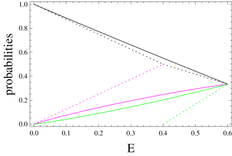
Figure 3: (Color online) The same as in Fig. 2, but now $\varepsilon_{1}=0$, $\varepsilon_{2}=0.8$ and $\varepsilon_{3}=1$. Dotted curves refer to the solution $\{12\}\vee\{23\}$ [see (52)], which is now the global minimum: $p_{1}$ (black), $p_{2}$ (magenta; note that $p_{2}=p_{3}$ for $E\geq\xi_{2}=\frac{\varepsilon_{2}}{2}=0.4$), and $p_{3}$ (green; we have $p_{3}=0$ for $E\leq\xi_{2}=\frac{\varepsilon_{2}}{2}=0.4$).

In this regime another strategy of risk-aversion is realized—the entropy-minimizing agent puts less weight on the highest-cost action. In particular, for $0\leq E\leq\frac{\varepsilon_{2}}{2}$ this action gets no probability at all: $p_{3}=0$; see (48). Hence when having two possibilities $\varepsilon_{2}$ and $\varepsilon_{3}$ with comparable high costs $\varepsilon_{2}\lesssim\varepsilon_{3}$, the agent prefers the lesser of two evils. In contrast, the entropy-maximizing agent will take these options with nearly equal probabilities. For larger values of $E$, the global minimum is $\{23\}$, where all probabilities are non-zero, but the probability for the action with the (intermediate) cost $\varepsilon_{2}$ is as large as for the least-cost action: $p_{2}=p_{1}$; see (49) and Figs. 1 and 3.

We see here an effect whose traces were also observed in the previous scenario: when choosing between two actions of comparable cost $\varepsilon_{2}\approx\varepsilon_{3}$, the entropy-minimizing agent is able to distinguish between them despite a small difference. In contrast to this, the entropy-maximizing agent will just take them with (approximately) equal probability, neglecting that small difference.

VI.4 Transitions from one regime to another, re-entrance, cognitive dissonance and frustration

VI.4.1 Transition between $\{13\}$ and $\{12\}$ upon increasing $E$

So far we studied cases $\varepsilon_{1}\approx\varepsilon_{2}\ll\varepsilon_{3}=1$ and $\varepsilon_{1}\ll\varepsilon_{2}\approx\varepsilon_{3}=1$, where one (global) solution—respectively, $\{13\}$ and $\{12\}\vee\{23\}$—provides the global entropy minimum for all values of $E$. Now we turn to studying cases, where $\varepsilon_{1}\not\approx\varepsilon_{2}$ and $\varepsilon_{3}\not\approx\varepsilon_{2}$. Here it is possible to have transitions between different local minima upon changing $E$; see Fig. 1 with the case $\varepsilon_{2}=0.33$.

For a sufficiently small $E$ the global minimum is $\{13\}$. But for $E>0.15$, the global minimum becomes $\{12\}$. This transition from one regime to another is continuous in terms of entropy, but discontinuous in terms of probabilities for various actions, as seen from (48–50). This is an analogue of the first-order phase transition in statistical physics systems (e.g., the liquid-vapor transition) balian , where the role of $E$ is played by the (physical) temperature. There the thermodynamic potential whose minimization determines stability (for our case this is entropy) changes continuously, but the order parameter (the difference between densities of liquid and vapor) suffers a discontinuous change balian .

The transition at $E=0.15$ is against naive intuition, because with a larger average cost $E$ the agent neglects the action $\varepsilon_{3}$, which is related to the highest cost. Here the agent who invests less into adaptation assigns more probability to costly actions. For the entropy-maximizing agent it is impossible that the probability of the most costly action decreases upon increasing $E$; cf. our discussion around (46). For the entropy-minimizing agent such an effect does take place—the probability $p_{3}$ of the most costly state changes from a positive value to zero—due to transition from one local minimum to another. For changes within the local minimum this cannot happen, as seen from (51–53). This effect can be related to cognitive dissonance disso ; aronson ; akela .

VI.4.2 Re-entrance

However, the above transition from $\{13\}$ to $\{12\}$ upon increasing $E$ is not the end of the story: at $E=0.165$ (and $\varepsilon_{2}=0.33$) the solution $\{12\}$ continuously (both in terms of entropy and probabilities) changes to $\{23\}$. This is a natural transition: for $E>0.165$, the solution $\{12\}$ does not exist anymore, since it cannot hold the constraint $E=p_{2}\varepsilon_{2}$; cf. (34). This is an analogue of a second-order phase transition in statistical physical systems (e.g., paramagnetic-ferromagnetic transition in magnets) balian , where one solution ceases to exist and is replaced by another via a continuous change of the order parameter (magnetization, in our case probabilities of actions).

But eventually, for $E>0.18$, the global minimum is back from $\{23\}$ to $\{13\}$ (re-entrance). The probabilities of the solution $\{13\}$ stay almost constant in the whole interval $0.15\leq E\leq 0.18$. Note that the re-entrance effect persists up to $\varepsilon_{2}\leq 0.45$. For $0.68>\varepsilon_{2}>0.45$ (not shown on figures) the re-entrance behavior is absent; there is only a single transition from $\{13\}$ to $\{12\}$ upon increasing $E$. Eventually, for $0.68<\varepsilon_{2}$ the global entropy minimum is always $\{12\}\vee\{23\}$, and we revert to the studied regime $\varepsilon_{1}\ll\varepsilon_{2}\approx\varepsilon_{3}=1$.

The transitions from $\{13\}$ to $\{12\}\vee\{23\}$ and back mean that there are three local minima with comparable values of entropy but different values for probabilities of actions; cf. Fig.1. They compete with each other upon relatively small changes of $E$. This effect resembles frustration, whose psychological content is that there are two (or more) different (incommensurate) goals or motivations that compete with one other. The concept of frustration is also well-known in statistical physics of complex systems (see kats for a recent review), where its meaning is very close to the above, since it relates to competing local minima of the thermodynamic potential (entropy in our case).

We stress that neither of the above effects is seen for the risk-seeking agent, because in this situation probabilities (38) are unique and depend smoothly on the parameters involved. This has to do with the fact that (38) was obtained via maximization of a concave function in a convex set, which generically produces unique and well-behaved results rock . Possible non-uniqueness of the Gibbs-Boltzmann probabilities (38) can show up only in the thermodynamic limit $n\to\infty$ for specific systems that can be subject to phase-transitions. (We however refrain from considering the $n\to\infty$ case, since it is far from an agent facing a limited amount of different choices.)

VI.5 Four actions

We turn to the entropy-minimizing scenarios for $n=4$. We do so briefly, because though $n=4$ is richer then $n=3$, it does not offer conceptual novelties. Here we also fix $\varepsilon_{1}=0$ and $\varepsilon_{4}=1$ [cf. (47)], and we are left with two parameters: $0<\varepsilon_{2}<\varepsilon_{3}<1$. For $\varepsilon_{2}\approx\varepsilon_{3}\approx 1$ the global minimum of entropy is provided by the solution $\{12\}\vee\{23\}\vee\{34\}$. It has the same meaning as above: among actions of comparable cost the risk-minimizing agent chooses the one with the lowest cost (i.e., $p_{2}>0$, but $p_{3}=p_{4}=0$) for $\xi_{1}\leq E\leq\xi_{2}$. Now this solution does not exist for $\xi_{2}\leq E\leq\xi_{3}$. In this regime the agent takes the solution $\{23\}$, where $p_{2}>0$, $p_{3}>0$, but $p_{4}=0$. For $\varepsilon_{2}\approx\varepsilon_{3}\ll 1$ the global minimum is $\{14\}$, as expected. Now $p_{2}=p_{3}=p_{4}>0$. These two regimes are similar to those for $n=3$. For $\varepsilon_{1}\approx\varepsilon_{2}\ll\varepsilon_{3}\approx\varepsilon_{4}$ the global minimum $\{14\}$ for a relatively low $E$ changes to $\{13\}\vee\{34\}$ for a large $E$. Finally, when both $\varepsilon_{2}$ and $\varepsilon_{3}$ are close to $0.5$, there is a sequence of transitions from one solution to another, such that every solution becomes a global minimum for a certain $E$; e.g., for $\varepsilon_{2}=0.4$ and $\varepsilon_{3}=0.5$ we observe the following transitions upon increasing $E$: $\{14\}\to\{12\}\to\{24\}\to\{23\}\to\{34\}$.

VII Summary and Discussion

An agent who wants to be adaptive in choosing between several actions in a varying and complex environment cannot exclusively focus on the least-cost action. The agent should also explore actions with non-minimal costs, and not only exploit the action with the minimal cost. This is the known exploration-exploitation trade-off, which exists in various forms and fields. We here worked out a set-up that allows us to study the trade-off within decision-making. The agent faces several actions, whose initial costs are known, but it is not known how they will change given the time and actions of the agent. Now the agent needs to perform several actions so that if there is a regular information about costs, then this information can be gathered. With which probabilities should he choose initial actions in such an agnostic situation?

We worked out one possibility, where the exploration goes via risk-minimization—a heuristic rule that people frequently apply in uncertain situations. Risk is a wide notion that appears in various situations. In particular, both risk-minimization (aversion) and risk-maximization are seen in experiments with people gambling on uncertain monetary outcomes baron .

In our situation the treatment of risk is easier than usual (cf. haim ; aumann ; leshno ) because we compare agents that have the same costs for their actions and decide to invest the same amount of average utility into exploration, i.e., into not taking the least-cost action only. We start with the stochastic dominance (or majorization) condition, which constraints specific risk measures. Given certain standard constraints, we show that the entropy can be employed as a measure of risk. This result is obtained via several different axiomatization schemes; see section III. Thus the risk-averse (risk-seeking) agent will minimize (maximize) the entropy given the average utility invested into adaptation, and also the constraint that more costly actions should get less probability. There are two different strategies of risk aversion: putting more probability on low-cost vs. high-cost actions. These strategies are different, and they relate to a rich behavior spectrum even in the simplest case of three actions.

While the entropy maximization is a well-known rule in probabilistic inference jaynes ; shore ; ttl ; uffink ; grun ; landes1 ; landes2 ; balian ; good ; christensen , the entropy minimization is an under-explored idea; cf. lindsay ; polgar ; jaynes_pra ; huhu ; karen ; good ; christensen . We show that this method can lead to useful predictions, e.g., it recovers (under definite conditions) the $\epsilon$-greedy probability known in reinforcement learning theory barto . Our main result is that the entropy-minimizing agent (in contrast to the entropy-maximizing one) shows certain aspects of intelligent behavior: (i) taking into account costly actions; (ii) choosing the best alternative among two comparable ones; (iii) cognitive dissonance.

Within (i) the entropy-minimizing (risk-averse) agent puts more probability into the least-cost action than the risk-seeking (entropy-maximizing) agent, and distributes the remainder such that the largest-cost action gets more probability than the risk-seeking agent; see (55, 55). Empirically, this scenario coincides with the $\epsilon$-greedy strategy known in reinforcement learning barto , but now it is derived—together with its validity conditions—from a more general principle of entropy minimization. Overall, this scenario resembles the behavior of a scientist who follows the incremental character of any science—hence devotes most of his time to traditional, low-cost subjects but is still open-minded enough to venture on alternatives that have higher costs of implementation and recognition.

When choosing between two actions with comparable cost, the entropy-minimizing agent chooses to put a higher probability on the lower-cost action; cf. (ii). We find this to be a (rudimentary) scientific attitude. The progress of science does relate to noting small differences in experiments and/or in theory; e.g. successful scientists are prone to see potential contradictions that are ignored by others. Also, modern theories of physics (e.g., quantum mechanics) are based on small experimental differences between their predictions and those of classical physics. In contrast, the entropy-maximizing agent gives approximately the same probability for actions with close costs.

The entropy-minimizing agent also demonstrates cognitive dissonance: by increasing the amount of utility $E$ invested into adaptation, this agent tends to nullify probabilities of high-cost actions. This effect relates to the fact that the minimization of entropy produces several local minima that compete with each other (frustration). Within the cognitive dissonance theory this effect is taken as a general sign of a loosely defined cognitive consistency. We relate it with risk-minimization.

We mention that maximizing the entropy of probability paths was proposed as a scheme for the emergence of intelligent behavior wissner . Though the mathematical details of the original proposal are unclear kappen , the proposal was generalized to social collective systems mann , and formalized within the convex analysis fry . We stress however that within the set-up studied here, the entropy maximization did not show features of intelligent behavior. Further work is needed to connect the presented research with the ones reported in wissner ; mann ; fry . There are also proposals of employing entropy minimization for improving the performance of machine learning algorithms kovach . Future research may clarify relations of this proposal with the presented results.

Another open problem is how to modify/continue the presented theory for applying it to problems of creativity modeling. One difference here is that in creative task solving it is the action space that has to be conceived and understood, while in various types of decision theories the action space is fixed. As examples show, even with this serious difference there are clear analogies between creative task solving and the exploration-exploitation dilemma.

Figure 1: (Color online) The locally minimal entropies $S_{\{12\}\vee\{23\}}(E)$ (red curves) and $S_{\{13\}}(E)$ (blue curves) as functions of $E$ for $n=3$; see (37). Using (47) we fixed for costs: $\varepsilon_{1}=0$, $0<\varepsilon_{2}<1$, and $\varepsilon_{3}=1$.
Dotted curves: $\varepsilon_{2}=0.1$. The blue curve is always lower: $S_{\{12\}\vee\{23\}}(E)>S_{\{13\}}(E)$; hence the local minimum $\{13\}$ is the global entropy minimum.
Full curves: $\varepsilon_{2}=0.33$. Now the blue and red curves intersect two times: the local minimum $\{13\}$ is not the global one for $0.15\leq E\leq 0.18$. The transition from $\{12\}$ to $\{23\}$ takes place at $E=0.165$.
Dashed curves: $\varepsilon_{2}=0.8$. Now the red curve is always lower, $S_{\{12\}\vee\{23\}}(E)<S_{\{13\}}(E)$, meaning that the solution $\{12\}\vee\{23\}$ is the global minimum.

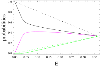
Figure 2: (Color online) Probabilities as a function of $E$ for the $n=3$ situation with $\varepsilon_{1}=0$, $\varepsilon_{2}=0.1$ and $\varepsilon_{3}=1$. Full curves: $\hat{p}_{1}$ (black), $\hat{p}_{2}$ (magenta), $\hat{p}_{3}$ (green). Dotted curves: $p_{1}$ (black), $p_{2}=p_{3}$ (green).
The Gibbs-Boltzmann probabilities $\hat{p}_{k}$ for the risk-seeking agent are calculated from (38). The probabilities $\{p_{k}\}_{k=1}^{3}$ refer to $\{13\}$ [see (53)], which is the global minimum for the present values of $\varepsilon_{k}$; cf. Fig. 1.

Appendix A Alternative route to constrained entropy optimization

The purpose of this Appendix is to outline an alternative method for obtaining entropy as a measure of risk and uncertainty; see (18). Recall that optimization (i.e., minimization or maximization) of entropy (16) under constraint (2) can be done via the optimization of the Lagrange function

$${\cal L}=-\sum_{k=1}^{n}p_{k}\ln p_{k}+\hat{\beta}\sum_{k=1}^{n}p_{k}\varepsilon_{k},$$ (60)

where $\hat{\beta}$ is the Lagrange multiplier that corresponds with $E$ in (2). Following aczel we shall mention an approach that allows us to recover directly (60) via few reasonable axioms. This is useful as an alternative (and more direct) route to optimizing entropy under (2).

Let us reinterpret actions ${\cal A}_{1},...,{\cal A}_{n}$ in (1) as events of a classical probability space. One seeks a measure ${\cal L}_{n}({\cal A}_{1},p_{1};...;{\cal A}_{n},p_{n})$ of uncertainty (or risk) that depends on both the probabilities and the corresponding events and that hold the following axioms aczel :

1. ${\cal L}_{n}({\cal A}_{1},p_{1};...;{\cal A}_{n},p_{n})$ is symmetric with respect to any permutation of $n$ elements $(z_{1},...,z_{n})$, where $z_{k}=({\cal A}_{k},p_{k})$.

2. ${\cal L}_{n}({\cal A}_{1},p_{1};...;{\cal A}_{n},p_{n})$ holds the branching feature

   $${\cal L}_{n}({\cal A}_{1},p_{1};...;{\cal A}_{n},p_{n})={\cal L}_{n-1}({\cal A}_{1}\cup{\cal A}_{2},p_{1}+p_{2};{\cal A}_{3},p_{3};...;{\cal A}_{n},p_{n})+(p_{1}+p_{2}){\cal L}_{2}({\cal A}_{1},\frac{p_{1}}{p_{1}+p_{2}};{\cal A}_{2},\frac{p_{2}}{p_{1}+p_{2}}).$$ (61)

   This is a natural feature for an uncertainty, where joining to events ${\cal A}_{1}$ and ${\cal A}_{2}$ (thus $p_{1}+p_{2}$ is the joint probability) leaves the residual uncertainty ${\cal L}_{2}({\cal A}_{1},\frac{p_{1}}{p_{1}+p_{2}};{\cal A}_{2},\frac{p_{2}}{p_{1}+p_{2}})$ with conditional probabilities $\frac{p_{1}}{p_{1}+p_{2}}$ and $\frac{p_{2}}{p_{1}+p_{2}}$ for ${\cal A}_{1}$ and ${\cal A}_{2}$, respectively.

3. ${\cal L}_{n}({\cal A}_{1},p_{1};...;{\cal A}_{n},p_{n})$ is a continuous function of $p_{1},p_{2},...,p_{n}$.

The three axioms lead to aczel :

$${\cal L}_{n}({\cal A}_{1},p_{1};...;{\cal A}_{n},p_{n})=-\sum_{k=1}^{n}p_{k}\ln p_{k}+\hat{\gamma}\sum_{k=1}^{n}p_{k}\varepsilon_{k}({\cal A}_{k}),$$ (62)

where $\varepsilon_{k}({\cal A}_{k})$ is an arbitrary function of ${\cal A}_{k}$, and $\hat{\gamma}$ is an arbitrary constant. (An irrelevant additive constant was fixed to zero). Interpreting $\varepsilon_{k}({\cal A}_{k})$ as the cost related to ${\cal A}_{k}$, and equating $\hat{\gamma}=\hat{\beta}$ we revert from (62) to (60). Eq. (62) and many related results can be proved via the functional equations methods reviewed in ali .

Note, that expressions similar to (62), i.e., a convex combination of entropy and expected cost (negative utility) were proposed in chin1 ; chin2 as a measure of risk. Refs. chin1 ; chin2 employ this measure for elucidating several controversies in the decision theory. The same measure was axiomatically deduced and studied in ng . Taking into account the axiomatic development, one can say that the measure of risk (62) expressed by a linear combination of entropy and expected cost does have normative features.

Appendix B Local minimality of solutions (29).

The aim of this Appendix is to show that the solutions for entropy minimization given by (29) do provide local minima of entropy. This is an important point, because once the local minimality is established, the solutions become meaningful even if they do not provide the global entropy minimum. To illustrate ideas, we start with the simplest non-trivial situation.

B.1 $n=3$

To check the local minimality we represent the probabilities of different actions as [see (22)]

$$p_{1}=\mu_{1}+\frac{\mu_{2}}{2}+\frac{\mu_{3}}{3}+\lambda_{1}+\frac{\lambda_{2}}{2}+\frac{\lambda_{3}}{3},$$ (63)

$$p_{2}=\frac{\mu_{2}}{2}+\frac{\mu_{3}}{3}+\frac{\lambda_{2}}{2}+\frac{\lambda_{3}}{3},$$ (64)

$$p_{3}=\frac{\mu_{3}}{3}+\frac{\lambda_{3}}{3},$$ (65)

$$p_{1}\geq p_{2}\geq p_{3},$$ (66)

where the unperturbed probabilities are [see (25, 26)]

$$\lambda_{1}+\lambda_{2}+\lambda_{3}=1,$$ (67)

$$\lambda_{1}\xi_{1}+\lambda_{2}\xi_{2}+\lambda_{3}\xi_{3}=E,$$ (68)

and where small perturbations $\mu_{k}$ hold

$$\mu_{1}+\mu_{2}+\mu_{3}=0,$$ (69)

$$\mu_{1}\xi_{1}+\mu_{2}\xi_{2}+\mu_{3}\xi_{3}=0.$$ (70)

We recall from (33) that

$$\xi_{1}\leq\xi_{2}\leq\xi_{3}.$$ (71)

To check the local minimality of the first solution we take $\lambda_{2}=0$ in (63–65). Now (66) demands [in addition to (69, 70)]

$$\mu_{2}>0.$$ (72)

Now we have for the entropy changes due to the perturbation:

$$\Delta S = -\sum_{k=1}^{3}p_{k}\ln p_{k}+\sum_{k=1}^{3}p_{k}|_{\mu_{l}=0}\ln p_{k}|_{\mu_{l}=0}$$ (73)

$$= -\sum_{k=1}^{3}(p_{k}-p_{k}|_{\mu_{l}=0})\ln p_{k}|_{\mu_{l}=0}$$ (74)

$$= -(\mu_{1}+\frac{\mu_{2}}{2}+\frac{\mu_{3}}{3})\ln\left[\frac{p_{1}|_{\mu_{l}=0}}{p_{2}|_{\mu_{l}=0}}\right]$$ (75)

$$= \frac{2\mu_{2}}{3}\left[\frac{\xi_{3}-\xi_{2}}{\xi_{3}-\xi_{1}}-\frac{1}{4}\right]\ln\left[\frac{p_{1}|_{\mu_{l}=0}}{p_{2}|_{\mu_{l}=0}}\right],$$ (76)

where in (74) we kept only the linear order over $\mu_{l}$, and where we employed (69, 70) in (75) and in (76). Due to (72) and to $\ln\left[\frac{p_{1}|_{\mu_{l}=0}}{p_{2}|_{\mu_{l}=0}}\right]\geq 0$, we get that $\Delta S>0$ (we are looking for the local minimum of entropy) is achieved for

$$\frac{\xi_{3}-\xi_{2}}{\xi_{3}-\xi_{1}}>\frac{1}{4}.$$ (77)

This inequality always holds, once one recalls the definition of $\xi_{k}$; see (26, 4).

To check the local minimality of the second solution we take $\lambda_{1}=0$ in (63–65). Now (66) demands [in addition to (69, 70)]

$$\mu_{1}>0.$$ (78)

Repeating the same steps as in (73–76), we get

$$\Delta S=\frac{\mu_{1}}{3}\,\frac{\xi_{2}-\xi_{1}}{\xi_{3}-\xi_{2}}\,\ln\left[\frac{p_{2}|_{\mu_{l}=0}}{p_{3}|_{\mu_{l}=0}}\right]>0,$$ (79)

i.e. this solution is local minimum (without additional conditions) due to (78), $\ln\left[\frac{p_{2}|_{\mu_{l}=0}}{p_{3}|_{\mu_{l}=0}}\right]>0$ and (71).

For the third solution we take $\lambda_{3}=0$ in (63–65). Now (66) demands [in addition to (69, 70)]

$$\mu_{3}>0.$$ (80)

We get instead of (79)

$$\Delta S={\cal O}(\mu_{3})+\frac{\mu_{3}}{3}\,\ln\left[\frac{3\,e\,p_{2}|_{\mu_{l}=0}}{\mu_{3}}\right]>0.$$ (81)

This expression is always non-negative, whenever $\mu_{3}>0$ is sufficiently small. Thus all solutions are always local minima.

B.2 $n>3$

We now turn to the more general situation and write probabilities as

$$p_{k}=\sum_{l=k}^{n}\frac{\mu_{l}}{l}+\sum_{l=k}^{n}\frac{\lambda_{l}}{l},\qquad k=1,...,n,$$ (82)

$$p_{1}\geq p_{2}\geq...\geq p_{n},$$ (83)

$$\sum_{l=k}^{n}\mu_{l}=0,$$ (84)

$$\sum_{l=k}^{n}\xi_{l}\mu_{l}=0,$$ (85)

where $\mu_{l}$ are perturbations. Now the unperturbed solution is defined by only two non-zero elements in $\{\lambda_{\alpha}\}_{\alpha=1}^{n}\geq 0$: $\lambda_{\alpha}$ and $\lambda_{\beta}$. Eq. (83) then implies that besides $\mu_{\alpha}$ and $\mu_{\beta}$ all other $\mu_{k}$ are necessarily non-negative:

$$\mu_{k}\geq 0,\qquad k\not=\alpha,\qquad k\not=\beta.$$ (86)

Using (84, 85), $\mu_{\alpha}$ and $\mu_{\beta}$ are expressed as

$$\mu_{\alpha}=\sum_{k=1,k\not=\alpha,k\not=\beta}^{n}\mu_{k}\frac{\xi_{k}-\xi_{\beta}}{\xi_{\beta}-\xi_{\alpha}},\qquad\mu_{\beta}=\sum_{k=1,k\not=\alpha,k\not=\beta}^{n}\mu_{k}\frac{\xi_{k}-\xi_{\alpha}}{\xi_{\alpha}-\xi_{\beta}}.$$ (87)

Eqs. (87) imply that if at least one $p_{k}|_{\mu_{l}=0}$ equals to zero, the corresponding solution is locally stable via the same mechanism as in (81).

Solutions for which $p_{k}|_{\mu_{l}=0}>0$ can be studied on the case-by-case basis. For the solution with $\lambda_{1}>0$ and $\lambda_{n}>0$ we obtain from (87) [cf. (73)]:

$$\Delta S = -\sum_{k=1}^{n}(p_{k}-p_{k}|_{\mu_{l}=0})\ln p_{k}|_{\mu_{l}=0}$$ (88)

$$= \ln\left[\frac{p_{1}|_{\mu_{l}=0}}{p_{2}|_{\mu_{l}=0}}\right]\,\frac{n-1}{n}\,\sum_{k=2}^{n-1}\mu_{k}\left\{\frac{\xi_{n}-\xi_{k}}{\xi_{n}-\xi_{1}}-\frac{n-k}{k(n-1)}\right\}$$ (89)

Now using (26, 4) for $\xi_{k}$ one can show directly that all the curly brackets in (89) are non-negative, which together with (86) and (83) implies $\Delta S\geq 0$, i.e., this solution is a local minimum of entropy. Generalizing this argument we converge to a conclusion that all the solutions are local minima.

References

- (1) D. Luce and H. Raiffa, Games and Decisions, (Wiley, New York, 1957).
- (2) R. Jeffrey, The Logic of Decision (2nd edition, Chicago University Press, Chicago, 1983).
- (3) R.S. Sutton and A.G. Barto, Reinforcement learning: an introduction (MIT Press, Cambridge, 1998).
- (4) J. D. Cohen, S. M. McClure, and A. J. Yu, Should I stay or should I go? How the human brain manages the trade-off between exploitation and exploration, Philosophical Transactions of the Royal Society B: Biological Sciences, 362, 933 (2007). J. G. March, Organization Science, Exploration and exploitation in organizational learning, 2, 71-87 (1991).
- (5) A.K. Gupta, K.G. Smith, and C.E. Shalley, Academy of Management Journal, 49, 693-706 (2006).
- (6) Handbook of Creativty, edited by R.J. Sternberg (Cambridge University Press, NY, 2009).
- (7) N.R.F. Maier, An aspect of human reasoning, British J. Psychol. 24, 144-155 (1933).
- (8) A. Luchins and E. Luchins, Mechanization in problem solving: The effect of Einstellung, Psychological Monographs 54(6) (1942).
- (9) L.L. Lopes, Between hope and fear: The psychology of risk, Advances in experimental social psychology, 20, 255-295 (1987).
- (10) L.L. Lopes, Re-Modelling Risk Aversion, in G. M. von Furstenberg (ed), Acting Under Uncertainty: Multidisciplinary Conceptions (Kluwer, Dordrecht 1990).
- (11) R. Pope, Towards a more precise decision framework, Theory and Decision 39, 241 (1995).
- (12) J. Baron, Thinking and deciding (Cambridge University Press, Cambridge, 2008).
- (13) R.T. Rockafellar, Convex Analysis (Princeton University Press, Princeton, NJ, 1970).
- (14) A. Gibbard and W. Harper, Two kinds of expected utility, in Ifs edited by W. Harper (pp. 153 190) (D. Reidel, Dordrecht, 1981).
- (15) J. Joyce and A. Gibbard, Causal Decision Theory, in Handbook of Utility Theory (Volume 1: Principles), edited by S. Barbera, P. Hammond, and C Seidl, (pp. 627 666) (Kluwer Academic Publishers, Dordrecht, 1998).
- (16) B. Skyrms, Darwin meets the “Logics of Decision”: Correlation in evolutionary game theory, Philosophy of Science, 61, 503 (1994).
- (17) B. Skyrms, Ratifiability and the “Logic of Decision”, Midwest studies in philosophy, 15, 44, (1990).
- (18) M. J. Shaffer, Decision Theory, Intelligent Planning and Counterfactuals, Minds & Machines, 19, 61 (2009).
- (19) A. Lenard, Thermodynamical proof of the Gibbs formula for elementary quantum systems, Journal of Statistical Physics, 19, 575 (1978).
- (20) V.I. Yukalov, D. Sornette, Self-organization in complex systems as decision making, Adv. Complex Syst. 17, 1450016 (2014).
- (21) A.E. Abbas, Maximum entropy utility, Operations Research, 54, 277 (2006).
- (22) H. Levy, Stochastic dominance and expected utility: survey and analysis, Management Science 38, 555 (1992).
- (23) R.J. Aumann and R. Serrano, An Economic Index of Riskiness, Journal of Political Economy, 116, 810 (2008). D.P. Foster and S. Hart, Journal of Political Economy, An operational measure of riskiness, 117, 785 (2009).
- (24) M. Leshno and H. Levy, Preferred by ”All” and Preferred by ”Most” Decision Makers: Almost Stochastic Dominance, Management Science, 48, 1074 (2002).
- (25) D. Kahneman and A. Tversky, Prospect theory: An analysis of decision under risk, Econometrica, 47, 263 (1979). A. Tversky and D. Kahneman, Advances in prospect theory: Cumulative representation of uncertainty, Journal of Risk and Uncertainty 5, 297 (1992).
- (26) T. Breuer and I. Csiszar, Measuring distribution model risk, Mathematical Finance, 26, 395 (2016).
- (27) A. Ahmadi-Javid, Entropic Value-at-Risk: A New Coherent Risk Measure, Journal of Optimization Theory and Applications, 155, 1105 (2012).
- (28) E.T. Jaynes, Violation of Boltzmann’s H theorem in real gases, Physical Review A, 4, 747 (1971).
- (29) C. Hu, Anti-H-theorem in Markov processes, Physical Review A, 34, 596 (1986). B. Crell, Comment on ”Anti-H-theorem in Markov processes”, Physical Review A, 39, 911 (1989).
- (30) M. Perarnau-Llobet, K V. Hovhannisyan, M. Huber, P. Skrzypczyk, J. Tura, and A. Acin, Most energetic passive states, Physical Review E, 92, 042147 (2015).
- (31) E.T. Jaynes, Prior probabilities, IEEE Trans. Syst. Science & Cybernetics 4, 227 (1968).
- (32) J.E. Shore and R.W. Johnson, Axiomatic derivation of the principle of maximum entropy and the principle of minimum cros-entropy, IEEE Trans. Info. Theory, IT-26, 26 (1980); ibid. IT-29, 942 (1980).
- (33) Y. Tikochinsky, N.Z. Tishby, and R.D. Levine, Consistent inference of probabilities for reproducible experiments, Physical Review Letters, 52, 1357 (1984).
- (34) J. Uffink, Can the maximum entropy principle be explained as a consistency requirement? Studies in History and Philosophy of Science B, 26, 223 (1995).
- (35) P. D. Grunwald and A. P. Dawid, Game theory, maximum entropy, minimum discrepancy and robust Bayesian decision theory, Annals of Statistics, 32, 1367 (2004).
- (36) J. Landes, Probabilism, Entropies and Strictly Proper Scoring Rules, International Journal of Approximate Reasoning, 63, 1 (2015).
- (37) J. Landes and J. Williamson, Objective Bayesianism and the maximum entropy principle, Entropy, 15, 3528 (2013).
- (38) R. Balian, From microphysics to macrophysics, I (Springer, Berlin, 2007).
- (39) I.J. Good, Some Statistical Methods in Machine Intelligence Research, Mathematical Biosciences, 6, 185 (1970).
- (40) R. Christensen, Entropy Minimax Multivariate Statistical Modeling I: Theory, International Journal of General Systems, 11, 231 (1985).
- (41) S. Watanabe, Information-theoretical aspects of inductive and deductive inference, IBM Journal of Research and Development, 4, 208 (1960).
- (42) S.N. Durlauf, How can statistical mechanics contribute to social science?, Proceedings of the National Academy of Sciences, 96, 10582 (1999).
- (43) D. H. Wolpert, M. Harre, E. Olbrich, N. Bertschinger, and J. Jost, Hysteresis effects of changing the parameters of noncooperative games, Physical Review E 85, 036102 (2012).
- (44) A. Kianercy and A. Galstyan, Dynamics of Boltzmann Q-learning in two-player two-action games, Physical Review E 85, 041145 (2012).
- (45) J.B. Paris and A. Vencovska, On the applicability of maximum entropy to inexact reasoning, International Journal of Approximate Reasoning, 1, 1 (1989).
- (46) J.B. Paris and A. Vencovska, A note on the inevitability of maximum entropy, International Journal of Approximate Reasoning, 4, 183 (1990).
- (47) D. Hunter, Causality and maximum entropy updating, International Journal of Approximate Reasoning, 3, 87 (1989).
- (48) G. Kern-Isberner, A note on conditional logics and entropy, International journal of approximate reasoning, 19, 231 (1998).
- (49) L.I. Rozonoer, Economics and Thermodynamics III, Automation and Remote Control, 34, 1272 (1973).
- (50) W. M. Saslow, An economic analogy to thermodynamics, American Journal of Physics 67, 1239 (1999).
- (51) J.C. Candeal, J.R. De Miguel, E. Indura, G.B. Mehta, Utility and entropy, Economic Theory, 17, 233 (2001).
- (52) J. Aczél and Z. Daróczy, A mixed theory of information I, RAIRO. Informatique théorique, 12, 149 (1978).
- (53) A.E. Abbas and J. Aczél, The role of some functional equations in decision analysis, Decision Analysis 7, 215 (2010),
- (54) J. Yang and W. Qiu, A measure of risk and a decision-making model based on expected utility and entropy, European Journal of Operational Reserch, 164, 792 (2005).
- (55) J. Yang and W. Qiu, Normalized Expected Utility-Entropy Measure of Risk, Entropy, 16, 3590 (2014).
- (56) R.D. Luce, C.T. Ng, A.A.J. Marley, and J. Aczel, Utility of gambling I: Entropy modified linear weighted utility, Econ. Theory, 36, 1 (2008); Utility of gambling II: Risk, paradoxes, and data, ibid. 36, 165 (2008).
- (57) J. Swait and A.A.J. Marley, Probabilistic choice (models) as a result of balancing multiple goals, Journal of Mathematical Psychology 57, 1 (2013).
- (58) R.B. Lindsay, Entropy consumption and values in physical science, American Scientist, 47, 376 (1959).
- (59) S. Polgar, Evolution and the thermodynamic imperative, Human Biology, 33, 99, (1961).
- (60) L. Festinger, A Theory of Cognitive Dissonance (Stanford University Press, Stanford, CA, 1957).
- (61) E. Aronson, The Social Animal (Palgrave Macmillan, 10th revised edition, 2007).
- (62) G. Akerlof and W.T. Dickens, The economic consequences of cognitive dissonance, American Economic Review, 72, 307 (1982).
- (63) A.E. Allahverdyan and A. Galstyan, Opinion Dynamics with Confirmation Bias, PLoS ONE 9, e99557 (2014).
- (64) A. D. Wissner-Gross and C. E. Freer, Causal Entropic Forces, Physical Review Letters, 110, 168702 (2013).
- (65) H. J. Kappen, Comment: Causal entropic forces, arXiv:1312.4185v1.
- (66) R. P. Mann and R. Garnett, The entropic basis of collective behaviour, Journal of The Royal Society Interface, 12, 20150037 (2015).
- (67) R. L. Fry, Physical Intelligence and Thermodynamic Computing, Entropy, 19, 107 (2017).
- (68) D. Kovach, The Computational Theory of Intelligence: Information Entropy, arXiv:1412.7978v1.
- (69) A.W. Marshall and I. Olkin, Inequalities: Theory of Majorization and its Applications, (Academic Press, New York, 1979).
- (70) T.W. Chaundy and J. B. McLeod, On a functional equation, Edinburgh Mathematical Notes, 43, 7 (1960).
- (71) M. I. Katsnelson, Y. I. Wolf, and E. V. Koonin, Towards physical principles of biological evolution, Physica Scripta 93, 043001 (2018).
- (72) S. Presse, K. Ghosh, J. Lee, K.A. Dill, Nonadditive Entropies Yield Probability Distributions with Biases not Warranted by the Data, Physical Review Letters, 111, 180604 (2013).
- (73) I. Csiszar and J. Korner, Information Theory (Akademiai Kiado, Budapest, 1981).
- (74) I. Csiszar, Axiomatic Characterizations of Information Measures, Entropy, 10, 261 (2008).