A stabilized cut discontinuous Galerkin framework: I. Elliptic boundary value and interface problems.

Abstract

We develop a stabilized cut discontinuous Galerkin framework for the numerical solution of elliptic boundary value and interface problems on complicated domains. The domain of interest is embedded in a structured, unfitted background mesh in $\mathbb{R}^{d}$, so that the boundary or interface can cut through it in an arbitrary fashion. The method is based on an unfitted variant of the classical symmetric interior penalty method using piecewise discontinuous polynomials defined on the background mesh. Instead of the cell agglomeration technique commonly used in previously introduced unfitted discontinuous Galerkin methods, we employ and extend ghost penalty techniques from recently developed continuous cut finite element methods, which allows for a minimal extension of existing fitted discontinuous Galerkin software to handle unfitted geometries. Identifying four abstract assumptions on the ghost penalty, we derive geometrically robust a priori error and condition number estimates for the Poisson boundary value problem which hold irrespective of the particular cut configuration. Possible realizations of suitable ghost penalties are discussed. We also demonstrate how the framework can be elegantly applied to discretize high contrast interface problems. The theoretical results are illustrated by a number of numerical experiments for various approximation orders and for two and three-dimensional test problems.

1 Introduction

1.1 Background

A fundamental prerequisite for the finite element based numerical solution of partial differential equations (PDEs) is the generation of high quality meshes to resolve geometric domain features and to ensure a sufficiently accurate approximation of the unknown solution. But despite continuously growing computer power, the generation of meshes for realistic, complex three-dimensional domains can still be a challenging task that can easily account for large portions of the time, human and computing resources in the overall simulation work flow. In applications where the domain geometry is main subject of interest, e.g., in shape optimization problems [1, 2, 3], the need of frequent remeshing can be the major computational cost. When the domain boundary is exposed to large or even topological changes, for instances in large deformation fluid-structure interaction problems [4] or multiphase flows [5, 6, 7, 8], even modern mesh moving algorithms may break down and then a costly remeshing is the only resort. Even if the domain of interest is stationary but rather complex, creating a 3D high quality mesh is a computationally demanding task. For instance, the simulation of geological flow and transport problems requires a series of highly non-trivial preprocessing steps to transform geological image data into conforming domain discretizations which respect intricate geometric structures such as faults and large-scale networks of fractures [9]. Similar non-trivial preprocessing steps are necessary when mesh-based domain descriptions are generated from biomedical image data, e.g., when creating flow models [10], bone models [11] or tissue models [12]. As a possible remedy to the mesh generation challenges, so-called unfitted finite elements methods have gained much attention in recent years. The fundamental idea is to avoid creating meshes fitted to the domain boundary by simply embedding the domain inside an easy-to-create background mesh. This way, the geometry description is decoupled from the numerical approximation and hence, complex static or evolving geometry can be handled.

1.2 Earlier work

Starting with [13], Glowinski et al. presented several fictitious domain formulations for the finite element method [14, 15, 16] with applications to electromagnetics [13], elliptic equations [16], and mainly fluid related equations [13, 17, 18, 19, 20], focusing on flows around moving rigid bodies.

In [21], Moës et al. introduced the so-called eXtended finite element method (XFEM) to avoid remeshing during crack propagation by representing discontinuities within an single mesh element, Based on the partition of unity method (PUM) [22], the polynomial spaces in the elements cut by the crack are enriched. The idea was later picked up by many authors and extended to a variety of applications, including two-phase flows [23], dendritic solidification [24], shock capturing problems [25], fluid-structure interaction problems [26], and flow and transport in fractured porous media [27, 28]. For an early overview over XFEM and its applications, the reader is referred to [29] and the references therein.

Parallel to the XFEM methodology,  Hansbo and Hansbo [30] proposed an alternative unfitted finite element formulation to treat elliptic interface problems by imposing weak discontinuities within the elements using a variant of Nitsche’s method [31]. Optimal a priori error and a posteriori error estimates were derived, independent of the interface position. Soon after, the idea was extended to composite grids [32] and to linear elasticity problems with strong and weak discontinuities [33]. Later Areias and Belytschko [34] showed that the approach in [33] can be recast into a XFEM formulation with a Heaviside enrichment. To deal with incompressible elasticity, the approach from [33] was extended in [35] by considering a stabilized mixed formulation using $\mathbb{P}_{1}$ continuous displacements and $\mathbb{P}_{0}$ discontinuous pressures. A critical ingredient in the analysis was the extension of the jump penalty based pressure stabilization from the “physical” part of the faces to the entire faces, leading to the first “ghost penalty” stabilized unfitted finite element formulation. The key idea of employing ghost penalties to extend the control of the relevant norms from the physical domain to the entire active mesh then crystallized in a series of papers [36, 37, 38] proposing Lagrange multiplier and Nitsche-based, optimally convergent fictitious domain methods for the Poisson problem. Additionally, the condition numbers of the associated system matrices turned out to be insensitive to the particular cut configuration and scaled similiar with respect to the mesh size as their fitted mesh counterparts.

Building upon and extending these ideas, the cut finite element method (CutFEM) as a particular unfitted finite element framework has gained rapidly increasing attention in the science and engineering community, see [39, 40] for some recent overviews. A distinctive feature of the CutFEM approach is that it provides a general, theoretically founded stabilization framework which, roughly speaking, transfers stability and approximation properties from a finite element scheme posed on a standard mesh to its cut finite element counterpart. As a result, a wide range of problem classes has been treated including, e.g., elliptic interface problems [41, 42, 43], Stokes and Navier-Stokes type problems [44, 45, 46, 47, 48, 49, 50, 51, 52], two-phase and fluid-structure interaction problems [53, 6, 54, 55]. Building up on the seminal work by  Olshanskii et al. [56], Olshanskii and Reusken [57], stabilized CutFEMs and so-called TraceFEMs were also developed for surface and surface-bulk PDEs [58, 59, 60, 61, 62, 63, 64, 65]. As a natural application area, unfitted finite element methods have also been proposed for problems in fractured porous media [66, 27, 67, 68]. Finally, we also mention the finite cell method as another important instance of an unfitted finite element framework with applications to flow and mechanics problems [69, 71, 70], see [72] for a review and references therein.

In addition to the aforementioned unfitted continuous finite element methods, unfitted discontinuous Galerkin methods have successfully been devised to treat boundary and interface problems on complex and evolving domains [73, 74, 75], including flow problems with moving boundaries and interfaces [76, 77, 78, 79, 80]. In contrast to stabilized continuous cut finite element methods, in unfitted discontinuous Galerkin methods, troublesome small cut elements can be merged with neighbor elements with a large intersection support by simply extending the local shape functions from the large element to the small cut element. As inter-element continuity is enforced only weakly, no additional measures need to be taken to force the modified basis functions to be globally continuous. Consequently, cell merging in unfitted discontinuous Galerkin methods provides an alternative stabilization mechanism to ensure that the discrete systems are well-posed and well-conditioned. For a very recent extension of the cell merging approach to continuous finite elements, we refer to [81, 82]. Thanks to their favorable conservation and stability properties, unfitted discontinuous Galerkin methods remain an attractive alternative to continuous CutFEMs, but some drawbacks are the almost complete absence of numerical analysis except for [83, 84], the implementational labor to reorganize the matrix sparsity patterns when agglomerating cut elements, and the lack of natural discretization approaches for PDEs defined on surfaces.

Finally, we also point out that alternative discontinuous Galerkin method for PDEs on complicated domains have been devised by exploiting the possibility to use non-standard element geometries which allows for a more flexible meshing of complicated geometries, see, e.g., [85, 86, 87].

1.3 Novel contributions and outline of this paper

In this work, we initiate the development of a novel stabilized cut discontinuous Galerkin (cutDG) framework by extending the stabilization techniques from the continuous CutFEM approach to discontinuous Galerkin based discretizations. Such an approach allows for a minimally invasive extension of existing fitted discontinuous Galerkin software to handle unfitted geometries. Only additional quadrature routines need to be added to handle the numerical integration on cut geometries, and while not being a completely trivial implementation task, we refer to the numerous quadrature algorithms capable of higher order geometry approximation  [88, 75, 89, 90, 91] which have been proposed in the last 5 years. Additionally, with a suitable choice of the ghost penalty, the sparsity pattern associated with the final system matrix does not require any manipulation and is identical to its fitted DG counterpart.

To lay out the theoretical foundations in the most simple setting, we here introduce and analyze cutDGMs for elliptic boundary and interface problems in Section 2 and Section 3, respectively. Boundary and interface conditions are imposed weakly using Nitsche’s method, and the discrete bilinear forms are augmented with an abstract ghost penalty stabilization. Hyperbolic and advection dominant advection-diffusion-reaction problems are considered in [92], while in the upcoming work [93], we will combine the presented framework with extension of [94, 95] to introduce cutDGM for mixed-dimensional, coupled problems.

We start with the Poisson boundary problem as model problem in Section 2.2 followed by the presentation of a symmetric interior penalty based cutDGM in Section 2.3. In the course of our stability and a priori error analysis of the cutDGM for the Poisson boundary problem in Section 2.4–2.5, we identify two abstract assumptions on the ghost penalty to derive geometrically robust and optimal approximation properties. In contrast to continuous cutFEMs, those do not automatically guarantee that the condition number of the resulting linear system is insensitive to the particular cut configuration. We find two additional abstract assumptions, allowing us to prove geometrically robust condition number estimates in Section 2.6. Afterwards in Section 2.7, we discuss a number of possible ghost penalty realizations which satisfy our abstract assumptions for the considered piecewise polynomial space of order $p$. The discussion of cutDGM for the Poisson boundary problem concludes with a series of numerical results in two and three dimensions to corroborate our theoretical findings and to examine the effects and properties of the ghost penalties in detail, see Section 2.7. Finally, in Section 3, we demonstrate how the framework can easily be used to devise cutDGM for high contrast interface problems. After the presentation of the interface model and the corresponding cutDGM in Section 3.1 and Section 3.2, respectively, we derive optimal a priori estimates in a concise manner in Section 3.3, followed by a number of convergence rate experiments for low and high contrast interface problems presented in Section 3.4.

2 Elliptic boundary value problems

2.1 Basic notation

Throughout this work, $\Omega\subset\mathbb{R}^{d}$, $d=2,3$ denotes an open and bounded domain with piecewise smooth boundary $\partial\Omega$, while $\Gamma$ denotes a piecewise smooth manifold of codimension $1$ embedded into $\mathbb{R}^{d}$. For $U\in\{\Omega,\Gamma\}$ and $0\leqslant m<\infty$, $1\leqslant q\leqslant\infty$, let $W^{m,q}(U)$ be the standard Sobolev spaces consisting of those $\mathbb{R}$-valued functions defined on $U$ which possess $L^{q}$-integrable weak derivatives up to order $m$. Their associated norms are denoted by $\|\cdot\|_{m,q,U}$. As usual, we write $H^{m}(U)=W^{m,2}(U)$ and $(\cdot,\cdot)_{m,U}$ and $\|\cdot\|_{m,U}$ for the associated inner product and norm. If unmistakable, we occasionally write $(\cdot,\cdot)_{U}$ and $\|\cdot\|_{U}$ for the inner products and norms associated with $L^{2}(U)$, with $U$ being a measurable subset of $\mathbb{R}^{d}$. Any norm $\|\cdot\|_{\mathcal{P}_{h}}$ used in this work which involves a collection of geometric entities $\mathcal{P}_{h}$ should be understood as broken norm defined by $\|\cdot\|_{\mathcal{P}_{h}}^{2}=\sum_{P\in\mathcal{P}_{h}}\|\cdot\|_{P}^{2}$ whenever $\|\cdot\|_{P}$ is well-defined, with a similar convention for scalar products $(\cdot,\cdot)_{\mathcal{P}_{h}}$. Any set operations involving $\mathcal{P}_{h}$ are also understood as element-wise operations, e.g., $\mathcal{P}_{h}\cap U=\{P\cap U\;|\;P\in\mathcal{P}_{h}\}$ and $\partial\mathcal{P}_{h}=\{\partial P\;|\;P\in\mathcal{P}_{h}\}$ allowing for compact short-hand notation such as $(v,w)_{\mathcal{P}_{h}\cap U}=\sum_{P\in\mathcal{P}_{h}}(v,w)_{P\cap U}$ and $\|\cdot\|_{\mathcal{P}_{h}\cap U}=\sqrt{\sum_{P\in\mathcal{P}_{h}}\|\cdot\|_{P\cap U}^{2}}$. Finally, throughout this work, we use the notation $a\lesssim b$ for $a\leqslant Cb$ for some generic constant $C$ (even for $C=1$) which varies with the context but is always independent of the mesh size $h$ and the position of $\Gamma$ relative to the background $\mathcal{T}_{h}$.

2.2 Poisson problem

We consider the following model boundary value problem: given $f\in H^{1}(\Omega)$ and $g\in H^{1/2}(\Gamma)$, find $u:\Omega\to\mathbb{R}$ such that

$$-\Delta u =f\quad\mbox{in }\Omega,$$ (2.1a)

$$u =g\quad\mbox{on }\Gamma.$$ (2.1b)

Setting $V_{g}=\{v\in H^{1}(\Omega):v|_{\Gamma}=g\}$ and defining the bilinear and linear forms

$$a(u,v)=(\nabla u,\nabla v)_{\Omega},\qquad l(v)=(f,v)_{\Omega},$$ (2.2)

the weak or variational formulation of the strong problem (2.1a) is to seek $u\in V_{g}$ such that

$$a(u,v)=l(v)\quad\forall\,v\in V_{0}.$$ (2.3)

2.3 A cut discontinuous Galerkin method for the Poisson problem

Let $\widetilde{\mathcal{T}}_{h}$ be a quasi-uniform background mesh consisting of $d$-dimensional, shape-regular (closed) simplices $\{T\}$ covering $\overline{\Omega}$. As usual, we introduce the local mesh size $h_{T}=\operatorname{diam}(T)$ and the global mesh size $h=\max_{T\in\widetilde{\mathcal{T}}_{h}}\{h_{T}\}$. For $\widetilde{\mathcal{T}}_{h}$ we define the so-called active (background) mesh

$$\mathcal{T}_{h} =\{T\in\widetilde{\mathcal{T}}_{h}\;|\;\cap\Omega^{\circ}\neq\emptyset\},$$ (2.4)

and its submesh $\mathcal{T}_{\Gamma}$ consisting of all cut elements,

$$\mathcal{T}_{\Gamma} =\{T\in\widetilde{\mathcal{T}}_{h}\;|\;\cap\Gamma\neq\emptyset\}.$$ (2.5)

Note that since the elements $\{T\}$ are closed by definition, the active mesh $\mathcal{T}_{h}$ still covers ${\Omega}$. The set of interior faces in the active background mesh is given by

$$\mathcal{F}_{h} =\{F=T^{+}\cap T^{-}\;|\;T^{+},T^{-}\in\mathcal{T}_{h}\}.$$ (2.6)

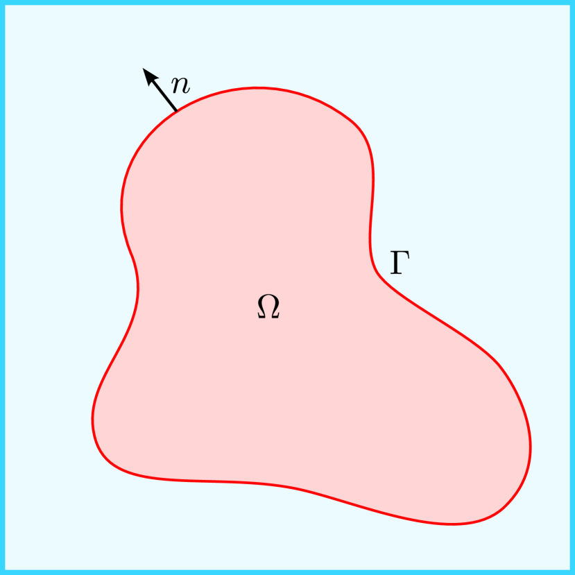
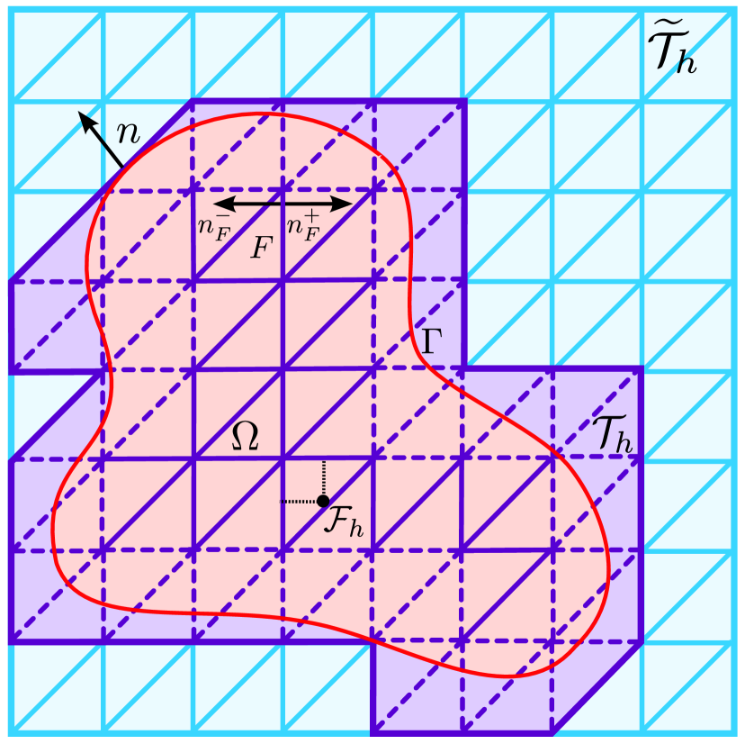
Figure 2.1: Computational domains for the boundary value problem (2.1). (Left) Physical domain $\Omega$ with boundary $\Gamma$ and outer normal $n$. (Right) Background mesh and active mesh used to define the approximation space. Faces on which the face based ghost penalty (2.97) is defined are plotted as dashed faces.

On the active mesh $\mathcal{T}_{h}$, we define the discrete function space $V_{h}$ as the broken polynomial space of order $k$,

$$V_{h}\coloneqq\mathbb{P}_{k}(\mathcal{T}_{h})\coloneqq\bigoplus_{T\in\mathcal{T}_{h}}\mathbb{P}_{k}(T).$$ (2.7)

To formulate our cut discontinuous Galerkin method for the boundary value problem (2.1), we recall the definition of the averages

$$\{{\sigma}\}|_{F} =\dfrac{1}{2}(\sigma_{F}^{+}+\sigma_{F}^{-}),$$ (2.8)

$$\{{n\cdot\sigma}\}|_{F} =\dfrac{1}{2}n\cdot(\sigma_{F}^{+}+\sigma_{F}^{-}),$$ (2.9)

and the jump across an interior face $F\in\mathcal{F}_{h}$,

$$[w]|_{F} =w_{F}^{+}-w_{F}^{-}.$$ (2.10)

Here, $w(x)^{\pm}=\lim_{t\rightarrow 0^{+}}w(x\pm tn)$ for some chosen unit facet normal $n$ on $F$.

Remark 2.1

To keep the notation at a moderate level, we usually do not use subscripts to indicate whether a normal belongs to a $F$ or to the boundary $\Gamma$ as it will be clear from context.

With these definitions in place, we can now define the discrete counterparts to the continuous bilinear and linear form (2.3) and set

$$a_{h}(v,w) =(\nabla v,\nabla w)_{\mathcal{T}_{h}\cap\Omega}-(\partial_{n}v,w)_{\Gamma}-(v,\partial_{n}w)_{\Gamma}+\beta(h^{-1}v,w)_{\Gamma}$$

$$\qquad-(\{{\partial_{n}v}\},[w])_{\mathcal{F}_{h}\cap\Omega}-([v],\{{\partial_{n}w}\})_{\mathcal{F}_{h}\cap\Omega}+\beta(h^{-1}[v],[w])_{\mathcal{F}_{h}\cap\Omega},$$ (2.11)

$$l_{h}(v) =(f,v)_{\mathcal{T}_{h}\cap\Omega}-(\partial_{n}v,g)_{\Gamma}+\beta(h^{-1}g,v)_{\Gamma},$$ (2.12)

for $v,w\in V_{h}$ where we used the short-hand notation $\partial_{n}v=n\cdot\nabla v$. The symmetric interior penalty based cut discontinuous Galerkin method for the Poisson problem (2.1) then reads: find $u_{h}\in V_{h}$ such that $\forall\,v\in V_{h}$

$$A_{h}(u_{h},v)\coloneqq a_{h}(u_{h},v)+g_{h}(u_{h},v)=l_{h}(v).$$ (2.13)

In contrast to the classical symmetric interior penalty method formulated on fitted meshes, we here augment the bilinear form $a_{h}$ with an additional stabilization form $g_{h}$, which is typically only active on elements in the vicinity of the embedded boundary $\Gamma$. The role of this stabilization is to ensure that, irrespective of the particular cut configuration, the bilinear form $A_{h}$ defined in (2.13) is coercive and bounded with respect to certain discrete energy-norms, and that the system matrix associated with $A_{h}$ is well-conditioned. To obtain these properties while maintaining the approximation qualities of original symmetric interior penalty method, the stabilization has to satisfy certain assumptions which we will extract from the forthcoming numerical analysis. Concrete realizations of $g_{h}$ are presented and discussed in Section 2.7.

Remark 2.2

The idea of augmenting an unfitted finite element scheme by certain stabilization forms acting in the vicinity of the boundary $\Gamma$ was first formulated in [38, 37] in the context of Nitsche-based fictitious domain methods for the Poisson problem employing continuous, piecewise polynomial ansatz functions. As realizations of $g_{h}$ typically require the evaluation of discrete functions $v\in V_{h}$ outside the physical domain $\Omega$, the term ghost penalty was coined in [38, 37, 35].

We conclude this section by formulating a few reasonable geometric assumptions on $\Gamma$ and $\mathcal{T}_{h}$, which allow us to keep the technical details the forthcoming numerical analysis at a moderate level.

Assumption G1

The boundary $\Gamma$ is of class $C^{2}$.

Assumption G2

The mesh $\mathcal{T}_{h}$ is quasi-uniform.

Finally, we require that $\Gamma$ is reasonably resolved by the active mesh $\mathcal{T}_{h}$. More specifically, for a boundary $\Gamma$ of class $C^{2}$ and its tubular neighborhood $U_{\delta}(\Gamma)=\{x\in\mathbb{R}^{d}:\operatorname{dist}(\Gamma,x)<\delta\}$ of radius $\delta$, it is well-known, that there is a $\delta_{0}>0$ such that $\forall\,x\in U_{\delta}(\Gamma)$, there is a unique closest point $p(x)$ on $\Gamma$ satisfying $|x-p(x)|=\operatorname{dist}(\Gamma,x)$, see, e.g, [96][Section 14.6]. We assume that $h<\delta_{0}$ such that $\mathcal{T}_{\Gamma}$ is contained in a tubular neighborhood for which such a closest point projection $p(x)$ is defined. In [43][Proposition 3.1] it was then shown that the following geometric assumption on the active mesh $\mathcal{T}_{h}$ is satisfied:

Assumption G3

For $T\in\mathcal{T}_{\Gamma}$ there is an element $T^{\prime}$ in $\omega(T)$ with a “fat” intersection such that

$$|T^{\prime}\cap\Omega|_{d}\geqslant c_{s}|T^{\prime}|_{d}$$ (2.14)

for some mesh independent $c_{s}>0$. Here, $\omega(T)$ denotes the set of elements sharing at least one node with $T$.

Remark 2.3

The assumed quasi-uniformity of $\mathcal{T}_{h}$ is mostly for notional convenience. Except for the condition number estimates, most given estimates can be easily localized to element or patch-wise estimates.

2.4 Stability properties

We start our theoretical investigation of the proposed cutDG method (2.13) by introducing various natural discrete norms and semi-norms. For $v\in V_{h}$ we define

$$|\mspace{-1.0mu}|\mspace{-1.0mu}|v|\mspace{-1.0mu}|\mspace{-1.0mu}|^{2}_{a_{h}} =\|\nabla v\|^{2}_{\mathcal{T}_{h}\cap\Omega}+\|h^{-1/2}[v]\|^{2}_{\mathcal{F}_{h}\cap\Omega},$$ (2.15)

$$|v|^{2}_{g_{h}} =g_{h}(v,v),$$ (2.16)

$$|\mspace{-1.0mu}|\mspace{-1.0mu}|v|\mspace{-1.0mu}|\mspace{-1.0mu}|^{2}_{A_{h}} =|\mspace{-1.0mu}|\mspace{-1.0mu}|v|\mspace{-1.0mu}|\mspace{-1.0mu}|^{2}_{a_{h}}+|v|^{2}_{g_{h}},$$ (2.17)

while for $v\in H^{2}(\mathcal{T}_{h})+V_{h}$, we will also consider the norm

$$|\mspace{-1.0mu}|\mspace{-1.0mu}|v|\mspace{-1.0mu}|\mspace{-1.0mu}|_{a_{h},\ast}^{2}=|\mspace{-1.0mu}|\mspace{-1.0mu}|v|\mspace{-1.0mu}|\mspace{-1.0mu}|_{a_{h}}^{2}+\|h^{\nicefrac{{1}}{{2}}}\{{\partial_{n}v}\}\|_{\mathcal{F}_{h}\cap\Omega}^{2}+\|h^{\nicefrac{{1}}{{2}}}\partial_{n}v\|_{\Gamma}^{2}.$$ (2.18)

Next, we show that the bilinear form $A_{h}$ is coercive and bounded with respect to the discrete energy norm $|\mspace{-1.0mu}|\mspace{-1.0mu}|\cdot|\mspace{-1.0mu}|\mspace{-1.0mu}|_{A_{h}}$. Recall that a pivotal ingredient in the numerical analysis of classical symmetric interior penalty method is the inverse inequality

$$\|\partial_{n}v\|_{F}\leqslant C_{I}h_{T}^{-\nicefrac{{1}}{{2}}}\|\nabla v\|_{T},$$ (2.19)

which holds for discrete functions $v\in\mathbb{P}_{k}(T)$ and $F\in\mathcal{F}_{T}\coloneqq\{F_{h}\in\mathcal{F}:F\subset\partial T\}$. Here, the inverse constant $C_{I}$ depends on the dimension $d$, the degree $k$ and the shape regularity of $T$. Unfortunately, a corresponding inverse inequality for the cut faces $F\cap\Omega\neq F$ of the form

$$\|\partial_{n}v\|_{F\cap\Omega}\leqslant C_{I}h_{T}^{-\nicefrac{{1}}{{2}}}\|\nabla v\|_{T\cap\Omega}$$

does not hold as the ratio $\tfrac{|F\cap\Omega|_{d-1}}{|T\cap\Omega|_{d}}$ between the $d-1$ dimensional surface area of the cut face $F\cap\Omega$ and the $d$-dimensional volume of the cut element $T\cap\Omega$ is highly dependent on the cut configuration; in fact, it can become arbitrarily large as illustrated by the “sliver case” in Figure 2.2.

Figure 2.2: Critical cut configurations. (Left): Sliver case. For $\delta\to 0$, the ratio $\tfrac{|\Gamma\cap T_{1}|_{d-1}}{|T_{1}\cap\Omega|_{d}}\sim\tfrac{h^{d}}{\delta h^{d-1}}$ can become arbitrarily large and thus the corresponding local inverse constant $C$ in (2.21) is practically unbounded. A similar observation holds for the ratio $\tfrac{|F_{1}|_{d-1}}{|T_{1}\cap\Omega|_{d}}$. (Right) Dotting case. Observe that for the faces $F_{x}$ and elements $T_{x}$ associated with node $x$, the corresponding face and element related contributions to the stiffness matrix associated with $a_{h}$ become arbitrarily small as $\delta\to 0$. Consequently, the stiffness matrix is almost singular and ill-conditioned if no proper ghost penalty is added.

As a partial replacement, one might be tempted to use simply the estimate

$$\|\partial_{n}v\|_{F\cap\Omega}\leqslant\|\partial_{n}v\|_{F}\leqslant C_{I}h_{T}^{-\nicefrac{{1}}{{2}}}\|\nabla v\|_{T}$$ (2.20)

instead. A similar issue arises when one wishes to control the normal flux on the boundary $\Gamma$ since an inequality of the form

$$\|\partial_{n}v\|_{\Gamma\cap T}\leqslant Ch_{T}^{-\nicefrac{{1}}{{2}}}\|\nabla v\|_{T\cap\Omega}$$ (2.21)

cannot hold with a constant $C$ which is independent of the cut configuration. Instead, we have only the inverse inequality

$$\|\partial_{n}v\|_{\Gamma\cap T}\leqslant Ch_{T}^{-\nicefrac{{1}}{{2}}}\|\nabla v\|_{T}$$ (2.22)

at our disposal, see [32] for a proof. Note that compared to constant $C_{I}$ in (2.20), the constant in (2.22) depends also on the local curvature of $\Gamma$. To fully exploit (2.20) and (2.22), it is necessary to extend the control of the $\|\nabla v\|^{2}_{\mathcal{T}_{h}\cap\Omega}$-part in natural energy norm $|\mspace{-1.0mu}|\mspace{-1.0mu}|\cdot|\mspace{-1.0mu}|\mspace{-1.0mu}|_{a_{h}}$ from the physical domain $\Omega$ to the entire active mesh $\mathcal{T}_{h}$. This is precisely one important role of the ghost penalty term $g_{h}$ which we formulate as our first assumption on $g_{h}$:

Assumption EP1

The ghost penalty $g_{h}$ extends the $H^{1}$ semi-norm from the physical domain $\Omega$ to the entire active mesh $\mathcal{T}_{h}$ in the sense that

$$\|\nabla v\|_{\mathcal{T}_{h}}^{2}\lesssim\|\nabla v\|_{\Omega}^{2}+|v|_{g_{h}}^{2}$$ (2.23)

holds for $v\in V_{h}$, with the hidden constants depending only on the dimension $d$, the polynomial order $k$ and the shape-regularity of $\mathcal{T}_{h}$.

An immediate result of our discussion is the following important corollary.

Corollary 2.4

Let $g_{h}$ satisfy EP1, then it holds that

$$\|h^{\nicefrac{{1}}{{2}}}\partial_{n}v\|_{\Gamma\cap\Omega}^{2}+\|h^{\nicefrac{{1}}{{2}}}\partial_{n}v\|_{\mathcal{F}_{h}\cap\Omega}^{2}\lesssim\|\nabla v\|_{\Omega}^{2}+|v|_{g_{h}}^{2}\lesssim|\mspace{-1.0mu}|\mspace{-1.0mu}|v|\mspace{-1.0mu}|\mspace{-1.0mu}|^{2}_{A_{h}}\quad\forall\,v\in V_{h},$$ (2.24)

with the hidden constants depending only on the dimension $d$, the polynomial order $k$, the shape-regularity of $\mathcal{T}_{h}$, and the curvature of $\Gamma$. In particular, we observe that

$$\|v|\mspace{-1.0mu}|\mspace{-1.0mu}|_{a_{h},\ast}\lesssim\|v|\mspace{-1.0mu}|\mspace{-1.0mu}|_{A_{h}}\quad\forall\,v\in V_{h}.$$ (2.25)

Having managed to control the normal flux on the cut geometries $\mathcal{F}_{h}\cap\Omega$ and $\Gamma\cap\Omega$, we can now prove the main result of this section.

Proposition 2.5

The discrete form $A_{h}$ is coercive and stable with respect to the discrete energy norm $|\mspace{-1.0mu}|\mspace{-1.0mu}|\cdot|\mspace{-1.0mu}|\mspace{-1.0mu}|_{A_{h}}$; that is,

$$|\mspace{-1.0mu}|\mspace{-1.0mu}|v|\mspace{-1.0mu}|\mspace{-1.0mu}|_{A_{h}}^{2} \lesssim A_{h}(v,v) \quad\forall\,v\in V_{h},$$ (2.26)

$$A_{h}(v,w) \lesssim|\mspace{-1.0mu}|\mspace{-1.0mu}|v\|_{A_{h}}\|v|\mspace{-1.0mu}|\mspace{-1.0mu}|_{A_{h}} \quad\forall\,v,w\in V_{h}.$$ (2.27)

Moreover, for $v\in H^{2}(\mathcal{T}_{h})+V_{h}$ and $w\in V_{h}$, the discrete form $a_{h}$ satisfies

$$a_{h}(v,w) \lesssim|\mspace{-1.0mu}|\mspace{-1.0mu}|v\|_{a_{h},\ast}\|v|\mspace{-1.0mu}|\mspace{-1.0mu}|_{A_{h}}.$$ (2.28)

Proof 1

Thanks to Corollary 2.4, the proof follows the standard arguments in the analysis of the classical symmetric interior penalty method. We start with (2.26). Setting $w=v$ in (2.13) and combining an $\epsilon$-Young inequality of the form $2ab\leqslant\epsilon a^{2}+\epsilon^{-1}b^{2}$ with the inverse estimates (2.20),(2.22), and Corollary 2.4, we see that

$$A_{h}(v,v) =\|\nabla v\|_{\Omega}^{2}+|v|_{g_{h}}^{2}+\beta\|h^{-\nicefrac{{1}}{{2}}}[v]\|_{\mathcal{F}_{h}}^{2}+\beta\|h^{-\nicefrac{{1}}{{2}}}v\|_{\Gamma}^{2}$$

$$\quad-2(\{{\partial_{n}v}\},[v])_{\mathcal{F}_{h}\cap\Omega}-2({\partial_{n}v},{v})_{\Gamma\cap\Omega}$$ (2.29)

$$\gtrsim\|\nabla v\|_{\Omega}^{2}+|v|_{g_{h}}^{2}+\beta\|h^{-\nicefrac{{1}}{{2}}}[v]\|_{\mathcal{F}_{h}}^{2}+\beta\|h^{-\nicefrac{{1}}{{2}}}v\|_{\Gamma}^{2}$$

$$\quad-\epsilon\|h^{\nicefrac{{1}}{{2}}}\{{\partial_{n}v}\}\|_{\mathcal{F}_{h}\cap\Omega}-\epsilon^{-1}\|h^{-\nicefrac{{1}}{{2}}}[v]\|_{\mathcal{F}_{h}\cap\Omega}-\epsilon\|h^{\nicefrac{{1}}{{2}}}{\partial_{n}v}\|_{\Gamma\cap\Omega}-\epsilon^{-1}\|h^{-\nicefrac{{1}}{{2}}}{v}\|_{\Gamma\cap\Omega}$$ (2.30)

$$\gtrsim(1-2\epsilon)\bigl{(}\|\nabla v\|_{\Omega}^{2}+|v|_{g_{h}}^{2}\bigr{)}+\bigl{(}\beta-\epsilon^{-1}\bigr{)}\bigl{(}\|h^{-\nicefrac{{1}}{{2}}}[v]\|_{\mathcal{F}_{h}}^{2}+\|h^{-\nicefrac{{1}}{{2}}}{v}\|_{\Gamma}^{2}\bigr{)}$$ (2.31)

$$\gtrsim|\mspace{-1.0mu}|\mspace{-1.0mu}|v|\mspace{-1.0mu}|\mspace{-1.0mu}|_{A_{h}}^{2}$$ (2.32)

if we choose $\epsilon>0$ small enough and $\beta\gtrsim\epsilon^{-1}$. To prove (2.27) and (2.28), simply apply a standard Cauchy-Schwarz inequality to see that terms involving the normal fluxes are bounded by

$$(\{{\partial_{n}v}\},[w])_{\mathcal{F}_{h}\cap\Omega}+({\partial_{n}v},{w})_{\Gamma\cap\Omega}\lesssim|\mspace{-1.0mu}|\mspace{-1.0mu}|v|\mspace{-1.0mu}|\mspace{-1.0mu}|_{a_{h},\ast}|\mspace{-1.0mu}|\mspace{-1.0mu}|w|\mspace{-1.0mu}|\mspace{-1.0mu}|_{a_{h},\ast}.$$ (2.33)

Then a further application of Corollary 2.4, Eq.(2.25) gives the desired estimates.

Remark 2.6

If the Dirichlet boundary condition (2.1b) is replaced by a natural boundary condition of Neuman or Robin type, the continuous cut finite element method version of (2.13) does not need any additional ghost penalty to guarantee discrete coercivity and optimal convergence of the method, but one can add a (more weakly scaled) ghost penalty to ensure robust condition numbers. In contrast, in the case of our cutDG formulation, a proper ghost penalty has to be added irrespective of the imposed boundary condition as the normal flux terms on cut faces also require the additional control formulated as Assumption EP1.

2.5 A priori error analysis

We turn the error analysis of the unfitted discretization scheme (2.13). To keep the technical details at a moderate level, we assume for a priori error analysis that the contributions from the cut elements $\mathcal{T}_{h}\cap\Omega$, the cut faces $\mathcal{F}_{h}\cap\Omega$ and the boundary parts $\Gamma\cap\mathcal{T}_{h}$ can be computed exactly. For a thorough treatment of variational crimes arising from the discretization of a curved boundary element methods, we refer the reader to [97, 98, 99].

Let us review some useful inequalities needed later and explain how to construct a suitable approximation operator. Recall that for $v\in H^{1}(\mathcal{T}_{h})$, the local trace inequalities of the form

$$\|v\|_{\partial T} \lesssim h_{T}^{-1/2}\|v\|_{T}+h_{T}^{1/2}\|\nabla v\|_{T}\quad\forall\,T\in\mathcal{T}_{h},$$ (2.34)

$$\|v\|_{\Gamma\cap T} \lesssim h_{T}^{-1/2}\|v\|_{T}+h_{T}^{1/2}\|\nabla v\|_{T}\quad\forall\,T\in\mathcal{T}_{h},$$ (2.35)

hold, see [32] for a proof of the second one. To construct a suitable approximation operator, we depart from the $L^{2}$-orthogonal projection $\pi_{h}:L^{2}(\mathcal{T}_{h})\to V_{h}$ which for $T\in\mathcal{T}_{h}$ and $F\in\mathcal{F}_{T}$ satisfies the error estimates

$$|v-\pi_{h}v|_{T,r} \lesssim h_{T}^{s-r}|v|_{s,T}, \quad 0\leqslant r\leqslant s,$$ (2.36)

$$|v-\pi_{h}v|_{F,r} \lesssim h_{T}^{s-r-\nicefrac{{1}}{{2}}}|v|_{s,T}, \quad 0\leqslant r\leqslant s-1/2,$$ (2.37)

whenever $v\in H^{s}(T)$. Now to lift a function $v\in H^{s}(\Omega)$ to $H^{s}(\Omega_{h}^{e})$, where we for the moment use the notation $\Omega_{h}^{e}=\bigcup_{T\in\mathcal{T}_{h}}T$, we recall that for Sobolev spaces $W^{m,q}(\Omega)$, $0<m\leqslant\infty,1\leqslant q\leqslant\infty$, there is a bounded extension operator satisfying

$$(\cdot)^{e}:W^{m,q}(\Omega)\to W^{m,q}(\Omega^{e}),\quad\|v^{e}\|_{m,q,\Omega^{e}}\lesssim\|v\|_{m,q,\Omega}$$ (2.38)

for $u\in W^{m,q}(\Omega)$, see [100] for a proof. After choosing some $\Omega^{e}$ such that $\Omega_{h,e}\subset\Omega^{e}\;\forall\,h\lesssim 1$, we can define an “unfitted” $L^{2}$ projection variant $\pi_{h}^{e}:H^{r}(\Omega_{h}^{e})\to V_{h}$ by setting

$$\pi_{h}^{e}v\coloneqq\pi_{h}v^{e}.$$ (2.39)

Note that this $L^{2}$-projection is slightly “perturbed” in the sense that it is not orthogonal on $L^{2}(\Omega)$ but rather on $L^{2}(\Omega_{h}^{e})$. Combining the local approximation properties of $\pi_{h}$ with the stability of the extension operator $(\cdot)^{e}$, we see immediately that $\pi_{h,\ast}$ satisfies the global error estimates

$$\|v-\pi_{h}^{e}v\|_{\mathcal{T}_{h},r} \lesssim h^{s-r}\|v\|_{s,\Omega}, \quad 0\leqslant r\leqslant s,$$ (2.40)

$$\|v-\pi_{h}^{e}v\|_{\mathcal{F}_{h},r} \lesssim h^{s-r-\nicefrac{{1}}{{2}}}\|v\|_{s,\Omega}, \quad 0\leqslant r\leqslant s-1/2,$$ (2.41)

$$\|v-\pi_{h}^{e}v\|_{\Gamma,r} \lesssim h^{s-r-\nicefrac{{1}}{{2}}}\|v\|_{s,\Omega}, \quad 0\leqslant r\leqslant s-1/2.$$ (2.42)

As a direct consequence, we can easily estimate the approximation error in the $|\mspace{-1.0mu}|\mspace{-1.0mu}|\cdot|\mspace{-1.0mu}|\mspace{-1.0mu}|_{a_{h},\ast}$-norm.

Corollary 2.7

Let $u\in H^{s}(\Omega)$ and assume that $V_{h}=P^{k}(\mathcal{T}_{h})$. Then for $r=\min\{s,k+1\}$, the approximation error of $\pi_{h}^{e}$ satisfies

$$|\mspace{-1.0mu}|\mspace{-1.0mu}|u-\pi_{h}^{e}u|\mspace{-1.0mu}|\mspace{-1.0mu}|_{a_{h},\ast}\lesssim h^{r-1}\|u\|_{r,\Omega}.$$ (2.43)

Proof 2

Set $e^{\pi}=u-\pi_{h}^{e}u$ and recall that

$$|\mspace{-1.0mu}|\mspace{-1.0mu}|u-\pi_{h}^{e}u|\mspace{-1.0mu}|\mspace{-1.0mu}|_{a_{h},\ast}^{2} =\|\nabla e^{\pi}\|^{2}_{\mathcal{T}_{h}\cap\Omega}+\|h^{-1/2}[e^{\pi}]\|^{2}_{\mathcal{F}_{h}\cap\Omega},+\|h^{\nicefrac{{1}}{{2}}}\{{\partial_{n}e^{\pi}}\}\|_{\mathcal{F}_{h}\cap\Omega}^{2}+\|h^{\nicefrac{{1}}{{2}}}\partial_{n}e^{\pi}\|_{\Gamma}^{2}$$ (2.44)

The first term can be simply estimated using (2.40), while estimate (2.41) gives the desired bounds for second. Finally, the last term can be treated by applying (2.42).

Before we formulate the main a priori error estimate, we need to quantify how the additional stabilization term $g_{h}$ affects the consistency of our method. First note that we have the following weak Galerkin orthogonality.

Lemma 2.8 (Weak Galerkin orthogonality)

Let $u\in H^{2}(\Omega)$ be the solution to (2.1) and let $u_{h}$ be the solution to the discrete formulation (2.13). Then

$$a_{h}(u-u_{h},v)=g_{h}(u_{h},v)\quad\forall\,v\in V_{h}.$$ (2.45)

Proof 3

Follows directly from the observation that $u$ satisfies $a_{h}(u,v)=l_{h}(v)\;\forall\,v\in V_{h}$.

Next, to assure that the remainder $g_{h}$ does not deteriorate the convergence order, we formulate our second assumption on the ghost penalty $g_{h}$.

Assumption EP2 (Weak consistency estimate)

For $v\in H^{s}(\Omega)$ and $r=\min\{s,k+1\}$, the semi-norm $|\cdot|_{g_{h}}$ satisfies the estimate

$$|\pi_{h}^{e}v|_{g_{h}}\lesssim h^{r-1}\|v\|_{r,\Omega}.$$ (2.46)

With these preliminaries in place, we can state and prove the main a priori error estimates.

Theorem 2.9 (A prior error estimates)

Let $u\in H^{s}(\Omega)$, $s\geqslant 2$ be the solution to (2.1) and let $u_{h}\in\mathbb{P}_{k}(\mathcal{T}_{h})$ be the solution to the discrete formulation (2.13). Then with $r=\min\{s,k+1\}$, the error $u-u_{h}$ satisfies

$$|\mspace{-1.0mu}|\mspace{-1.0mu}|u-u_{h}|\mspace{-1.0mu}|\mspace{-1.0mu}|_{a_{h},\ast} \lesssim h^{r-1}\|u\|_{r,\Omega},$$ (2.47)

$$\|u-u_{h}\|_{\Omega} \lesssim h^{r}\|u\|_{r,\Omega}.$$ (2.48)

Proof 4

With the “extended” $L^{2}$ projection $\pi_{h}^{e}$ and the proper cut variants of trace inequalities in place, the proof follows closely the standard arguments and is included only for completeness.

Estimate (2.47). First, we decompose the total error $e=u-u_{h}$ into a discrete error $e_{h}=\pi_{h}^{e}u-u_{h}$ and a projection error $e_{\pi}=u-\pi_{h}^{e}u$. Observe that $|\mspace{-1.0mu}|\mspace{-1.0mu}|u-u_{h}|\mspace{-1.0mu}|\mspace{-1.0mu}|_{a_{h}}\leqslant\|e_{\pi}|\mspace{-1.0mu}|\mspace{-1.0mu}|_{a_{h},\ast}+\|e_{h}|\mspace{-1.0mu}|\mspace{-1.0mu}|_{A_{h}}$ and thanks to Corollary 2.7, it is enough to estimate the discrete error. Combining the coercivity result (2.26) with the weak Galerkin orthogonality (2.45) and the boundedness (2.28) yields

$$|\mspace{-1.0mu}|\mspace{-1.0mu}|e_{h}|\mspace{-1.0mu}|\mspace{-1.0mu}|_{A_{h}}^{2} \lesssim a_{h}(\pi_{h}^{e}u-u_{h},e_{h})+g_{h}(\pi_{h}^{e}u-u_{h},e_{h})$$ (2.49)

$$=a_{h}(\pi_{h}^{e}u-u,e_{h})+g_{h}(\pi_{h}^{e}u,e_{h})$$ (2.50)

$$\lesssim\bigl{(}|\mspace{-1.0mu}|\mspace{-1.0mu}|\pi_{h}^{e}u-u|\mspace{-1.0mu}|\mspace{-1.0mu}|_{a_{h},\ast}+|\pi_{h}^{e}u|_{g_{h}}\bigr{)}\bigl{(}|\mspace{-1.0mu}|\mspace{-1.0mu}|e_{h}|\mspace{-1.0mu}|\mspace{-1.0mu}|_{a_{h},\ast}+|e_{h}|_{g_{h}}\bigr{)}$$ (2.51)

$$\lesssim h^{r-1}|\mspace{-1.0mu}|\mspace{-1.0mu}|u\|_{r,\Omega}|\mspace{-1.0mu}|\mspace{-1.0mu}|e_{h}|\mspace{-1.0mu}|\mspace{-1.0mu}|_{A_{h}},$$ (2.52)

where in the last step, the projection error estimate (2.43) was used again together with the consistency error assumption EP2 and the norm equivalence $|\mspace{-1.0mu}|\mspace{-1.0mu}|e_{h}|\mspace{-1.0mu}|\mspace{-1.0mu}|_{a_{h},\ast}+|e_{h}|_{g_{h}}\sim|\mspace{-1.0mu}|\mspace{-1.0mu}|e_{h}|\mspace{-1.0mu}|\mspace{-1.0mu}|_{A_{h}}$ valid for $e_{h}\in V_{h}$. Now dividing (2.52) by $|\mspace{-1.0mu}|\mspace{-1.0mu}|e_{h}|\mspace{-1.0mu}|\mspace{-1.0mu}|_{A_{h}}$ gives the desired estimate for the discrete error.

Estimate (2.48). As usual, we employ the Aubin-Nitsche duality trick, but we need to keep track of the weakly consistent ghost penalty $g_{h}$. Let $\psi\in L^{2}(\Omega)$, then thanks to assumption G1, there is a $\phi\in H^{2}(\Omega)\cap H_{0}^{1}(\Omega)$ satisfying $-\Delta\phi=\psi$ and the regularity estimate $\|\phi\|_{2,\Omega}\lesssim\|\psi\|_{\Omega}$. Since $\phi\in H^{2}(\Omega)\cap H_{0}^{1}(\Omega)$, an integration by parts argument shows that $(e,-\Delta\phi)_{\Omega}=a_{h}(e,\phi)$. Hence, recalling the weak Galerkin orthogonality (2.45), we see that

$$(e,\psi)_{\Omega} =a_{h}(e,\phi)$$ (2.53)

$$=a_{h}(e,\phi-\pi_{h}\phi)+g_{h}(u_{h},\pi_{h}\phi)$$ (2.54)

$$=a_{h}(e,\phi-\pi_{h}\phi)+g_{h}(u_{h}-\pi_{h}^{e}u,\pi_{h}\phi)+g_{h}(\pi_{h}^{e}u,\pi_{h}\phi)$$ (2.55)

$$\lesssim|\mspace{-1.0mu}|\mspace{-1.0mu}|u-u_{h}|\mspace{-1.0mu}|\mspace{-1.0mu}|_{a_{h},*}|\mspace{-1.0mu}|\mspace{-1.0mu}|\phi-\pi_{h}\phi|\mspace{-1.0mu}|\mspace{-1.0mu}|_{a_{h},*}+|\mspace{-1.0mu}|\mspace{-1.0mu}|\pi_{h}^{e}u-u_{h}|\mspace{-1.0mu}|\mspace{-1.0mu}|_{a_{h},*}|\pi_{h}\phi|_{g_{h}}+|\pi_{h}u|_{g_{h}}|\pi_{h}\phi|_{g_{h}}$$ (2.56)

$$\lesssim h^{r-1}\|u\|_{r,\Omega}h\|\phi\|_{2,\Omega}\lesssim h^{r}\|u\|_{r,\Omega}\|\psi\|_{\Omega},$$ (2.57)

where in the two last steps, a Cauchy-Schwarz inequality for the symmetric bilinear forms $a_{h}$ and $g_{h}$ was combined with the weak consistency assumption EP2, estimate (2.47) and the energy-norm estimate for the discrete error $\pi_{h}^{e}u-u_{h}$ derived in  (2.49)–(2.52). Consequently, we found that

$$\|u-u_{h}\|_{\Omega} =\sup_{\psi\in L^{2}(\Omega),\|\psi\|_{\Omega}=1}(e,\psi)_{\Omega}\lesssim h^{r}\|u\|_{r,\Omega}.$$ (2.58)

Remark 2.10

Note that since the proof of the $L^{2}$ error estimate is based on a duality argument, the employed ghost penalty is not required to extend the $L^{2}$ norm to actually guarantee optimal error estimates in the $L^{2}$ norm.

2.6 Condition number estimates

We conclude the theoretical analysis of the stabilized cutDGM for the Poisson problem by demonstrating how the addition of a suitably designed ghost penalty $g_{h}$ ensures that the condition number of the resulting stiffness matrix can be bounded by $\mathcal{O}(h^{-2})$, irrespective of how the boundary $\Gamma$ cuts the background mesh $\mathcal{T}_{h}$.

Let $\{\phi_{i}\}_{i=1}^{N}$ be the standard piecewise polynomial basis functions associated with $V_{h}=\mathbb{P}_{k}(\mathcal{T}_{h})$ so that any $v\in V_{h}$ can be writtes as $v=\sum_{i=1}^{N}V_{i}\phi_{i}$ with coefficients $V=\{V_{i}\}_{i=1}^{N}\in\mathbb{R}^{N}$. The stiffness matrix $\mathcal{A}$ is defined by the relation

$$(\mathcal{A}V,W)_{\mathbb{R}^{N}}=A_{h}(v,w)\quad\forall\,v,w\in V_{h}.$$ (2.59)

Thanks to the coercivity of $A_{h}$, the stiffness matrix $\mathcal{A}$ is a bijective linear mapping $\mathcal{A}:\mathbb{R}^{N}\to\mathbb{R}^{N}$ with its operator norm and condition number defined by

$$\|\mathcal{A}\|_{\mathbb{R}^{N}}=\sup_{V\in\widehat{\mathbb{R}}^{N}\setminus\boldsymbol{0}}\dfrac{\|\mathcal{A}V\|_{\mathbb{R}^{N}}}{\|V\|_{\mathbb{R}^{N}}}\quad\text{and}\quad\kappa(\mathcal{A})=\|\mathcal{A}\|_{\mathbb{R}^{N}}\|\mathcal{A}^{-1}\|_{\mathbb{R}^{N}},$$ (2.60)

respectively. Following the approach in [101], a bound for the condition number can be derived by combining three ingredients. The first one consists of the well-known estimate

$$h^{d/2}\|V\|_{\mathbb{R}^{N}}\lesssim\|v\|_{L^{2}(\mathcal{T}_{h})}\lesssim h^{d/2}\|V\|_{\mathbb{R}^{N}},$$ (2.61)

which holds for any quasi-uniform mesh $\mathcal{T}_{h}$ and $v\in V_{h}$, and allows us to pass between the discrete $l^{2}$ norm of coefficient vectors $V$ and the continuous $L^{2}$ norm of finite element functions $v_{h}$. Second, a discrete Poincaré-type estimate is needed to pass from the $L^{2}$ norm to the discrete energy-norm. Finally, we need an inverse inequality which enables us to bound the discrete energy norm by the $L^{2}$ norm.

2.6.1 Discrete Poincaré estimate

Recall that for the standard symmetric interior penalty method on fitted, quasi-uniform meshes, the discrete Poincaré inequality

$$\|v\|_{\mathcal{T}_{h}}\lesssim\|\nabla v\|_{\mathcal{T}_{h}}+\|h^{-\nicefrac{{1}}{{2}}}[u]\|_{\mathcal{F}_{h}}+\|h^{-\nicefrac{{1}}{{2}}}u\|_{\Gamma}$$ (2.62)

holds for $v\in V_{h}$, see [102, 103]. Proving such an inequality in the unfitted case is a slightly more subtle undertaking. First, to apply (2.61) when passing between discrete $l^{2}$ and continuous $L^{2}$-norms, we have to work again on the entire active mesh and not only on the physical part $\Omega$. In particular, $\Gamma$ does not longer constitutes the boundary of the domain under consideration as in (2.62). Second, note that the fictitious domain $\Omega_{h}^{e}$ associated with the active mesh $\mathcal{T}_{h}$ changes with decreasing mesh size. To gain control over the $L^{2}(\mathcal{T}_{h})$ and to be able to derive a suitable discrete Poincaré inequality leads us to the next assumption on $g_{h}$:

Assumption EP3

The ghost penalty $g_{h}$ extends the $L^{2}$ norm from the physical domain to the entire active mesh $\mathcal{T}_{h}$ in the sense that

$$\|v\|_{\mathcal{T}_{h}}^{2} \lesssim\|v\|_{\Omega}^{2}+|v|_{g_{h}}^{2},$$ (2.63)

holds for $v\in V_{h}$, with the hidden constants depending only on the dimension $d$, the polynomial order $k$ and the shape-regularity of $\mathcal{T}_{h}$.

Proposition 2.11 (Discrete Poincaré inequality)

For $v\in V_{h}$, it holds that

$$\|v\|_{\mathcal{T}_{h}}\lesssim|\mspace{-1.0mu}|\mspace{-1.0mu}|v|\mspace{-1.0mu}|\mspace{-1.0mu}|_{A_{h}}.$$ (2.64)

Proof 5

Since $\|v\|_{\mathcal{T}_{h}}\lesssim\|v\|_{\Omega}+|v|_{g_{h}}$ by Assumption EP3, the main task is to estimate $\|v\|_{\Omega}$, which can be done by combining the proof given [102] with the trace inequalities (2.34), (2.35) and the boundedness of the extension operator $(\cdot)^{e}:W^{m,p}(\Omega)\to W^{m,q}(\mathbb{R}^{d})$. More specifically, thanks to Assumption G1 and the implied elliptic regularity, there is a $\psi\in H^{2}(\Omega)\cap H^{1}_{0}(\Omega)$ satisfying $-\Delta\psi=v$ and $\|\psi^{e}\|_{2,\mathbb{R}^{d}}\lesssim\|v\|_{\Omega}$. Consequently,

$$\|v\|_{\Omega}^{2} =(v,-\Delta\psi)_{\Omega}$$ (2.65)

$$=(\nabla v,\nabla\psi)_{\Omega}-(v,\partial_{n}\psi)_{\Gamma}-([v],\{{\partial_{n}\psi}\})_{\mathcal{F}_{h}\cap\Omega}$$ (2.66)

$$\lesssim\bigl{(}\|\nabla v\|_{\Omega}+\|h^{-\nicefrac{{1}}{{2}}}v\|_{\Gamma}+\|h^{-\nicefrac{{1}}{{2}}}[v]\|_{\mathcal{F}_{h}\cap\Omega}\bigr{)}$$

$$\quad\cdot\bigl{(}\|\nabla\psi\|_{\Omega}+\|h^{\nicefrac{{1}}{{2}}}\partial_{n}\psi\|_{\Gamma}+\|h^{\nicefrac{{1}}{{2}}}\{{\partial_{n}\psi}\}\|_{\mathcal{F}_{h}\cap\Omega}\bigr{)}$$ (2.67)

$$\lesssim|\mspace{-1.0mu}|\mspace{-1.0mu}|v|\mspace{-1.0mu}|\mspace{-1.0mu}|_{a_{h}}\bigl{(}\|\nabla\psi^{e}\|_{\mathcal{T}_{h}}+h\|D^{2}\psi^{e}\|_{\mathcal{T}_{h}}\bigr{)}$$ (2.68)

$$\lesssim|\mspace{-1.0mu}|\mspace{-1.0mu}|v|\mspace{-1.0mu}|\mspace{-1.0mu}|_{a_{h}}\|v\|_{\Omega}$$ (2.69)

and thus $\|v\|_{\mathcal{T}_{h}}\lesssim\|v\|_{\Omega}+|v|_{g_{h}}\lesssim|\mspace{-1.0mu}|\mspace{-1.0mu}|v|\mspace{-1.0mu}|\mspace{-1.0mu}|_{a_{h}}+|v|_{g_{h}}\sim|\mspace{-1.0mu}|\mspace{-1.0mu}|v|\mspace{-1.0mu}|\mspace{-1.0mu}|_{A_{h}}$ which gives the desired bound.

Remark 2.12

We point out that in continuous cut finite element formulations for the Poisson problem as proposed in [38, 37], Assumption EP3 and thus Proposition 2.11 are automatically satisfied when Assumption EP1 holds, thanks to a standard Poincaré inequality of the form $\|v\|_{\Omega}\lesssim\|\nabla v\|_{\Omega}+\|v\|_{\Gamma}$ valid for $H^{1}$ conform elements.

2.6.2 Inverse inequalities

We note first that, similar to (2.22) and (2.20), we have the following inverse estimates for $v\in\mathbb{P}_{k}(T)$ and $F\in\mathcal{F}_{T}$,

$$\|\nabla v\|_{T\cap\Omega}\lesssim\|h^{-1}v\|_{T},\qquad\|v\|_{\Gamma\cap T}\lesssim\|h^{-\nicefrac{{1}}{{2}}}u\|_{T},\qquad\|u\|_{F\cap\Omega}\lesssim\|h^{-\nicefrac{{1}}{{2}}}u\|_{T}.$$ (2.70)

To prove the desired inverse estimate for the energy norm $|\mspace{-1.0mu}|\mspace{-1.0mu}|\cdot|\mspace{-1.0mu}|\mspace{-1.0mu}|_{A_{h}}$, it is natural to require that the ghost penalty itself satisfies the same type of inverse inequality:

Assumption EP4

For $v\in V_{h}$ it holds that

$$|v|_{g_{h}}\lesssim h^{-1}\|v\|_{\mathcal{T}_{h}},$$ (2.71)

with the hidden constant independent of the particular configuration.

Then combining the inverse estimates (2.70) with Assumption EP4, it is straightforward to prove the next lemma.

Lemma 2.13 (Inverse estimate for $|\mspace{-1.0mu}|\mspace{-1.0mu}|\cdot|\mspace{-1.0mu}|\mspace{-1.0mu}|_{A_{h}}$)

For $v\in V_{h}$, it holds

$$|\mspace{-1.0mu}|\mspace{-1.0mu}|v|\mspace{-1.0mu}|\mspace{-1.0mu}|_{A_{h}}\lesssim h^{-1}\|v\|_{\mathcal{T}_{h}}$$ (2.72)

with the hidden constant only depending on the dimension $d$, the polynomial degree $k$ and the shape regularity of $\mathcal{T}$, but not on the particular cut configuration.

Remark 2.14

Note again, that for a cut face with $F\cap T\subsetneq F$ (and similar for $\Gamma\cap T$), an inverse estimate of the form $\|v\|_{F\cap\Omega}\lesssim\|h^{-\nicefrac{{1}}{{2}}}v\|_{T\cap\Omega}$ cannot hold for arbitrary cut configurations, thus the application of the inverse estimates (2.70) forces us to pass from the physical domain $\Omega$ to the entire active mesh $\mathcal{T}_{h}$.

2.6.3 The condition number estimate

Finally, we combine the mass-matrix scaling (2.61), the discrete Poincaré inequality (2.64) and the inverse estimate (2.72) to derive a geometrically robust conditon number bound.

Theorem 2.15

The condition number of the stiffness matrix satisfies the estimate

$$\kappa(\mathcal{A})\lesssim h^{-2},$$ (2.73)

where the hidden constant depends only on the dimension $d$, the polynomial order $k$ and the quasi-uniformity of $\mathcal{T}_{h}$, but not on the particular cut configuration.

Proof 6

We need to bound $\|\mathcal{A}\|_{\mathbb{R}^{N}}$ and $\|\mathcal{A}^{-1}\|_{\mathbb{R}^{N}}$. First observe that for $w\in V_{h}$,

$$|\mspace{-1.0mu}|\mspace{-1.0mu}|w|\mspace{-1.0mu}|\mspace{-1.0mu}|_{A_{h}}\lesssim h^{-1}\|w\|_{\mathcal{T}_{h}}\lesssim h^{(d-2)/2}\|W\|_{\mathbb{R}^{N}},$$ (2.74)

where the inverse estimate (2.72) and equivalence (2.61) were successively used. Thus

$$\|\mathcal{A}V\|_{\mathbb{R}^{N}} =\sup_{W\in\mathbb{R}^{N}\setminus\{0\}}\frac{(\mathcal{A}V,W)_{\mathbb{R}^{N}}}{\|W\|_{\mathbb{R}^{N}}}=\sup_{w\in V_{h}\setminus\{0\}}\frac{A_{h}(v,w)}{|\mspace{-1.0mu}|\mspace{-1.0mu}|w|\mspace{-1.0mu}|\mspace{-1.0mu}|_{A_{h}}}\frac{|\mspace{-1.0mu}|\mspace{-1.0mu}|w|\mspace{-1.0mu}|\mspace{-1.0mu}|_{A_{h}}}{\|W\|_{\mathbb{R}^{N}}}$$ (2.75)

$$\lesssim h^{(d-2)/2}|\mspace{-1.0mu}|\mspace{-1.0mu}|v|\mspace{-1.0mu}|\mspace{-1.0mu}|_{A_{h}}\lesssim h^{d-2}\|V\|_{\mathbb{R}^{N}},$$ (2.76)

and thus $\|\mathcal{A}\|_{\mathbb{R}^{N}}\lesssim h^{d-2}$ by the definition of the operator norm. To estimate $\|\mathcal{A}^{-1}\|_{\mathbb{R}^{N}}$, start from (2.61) and combine the Poincaré inequality (2.64) with a Cauchy-Schwarz inequality to arrive at the following chain of estimates:

$$\|V\|^{2}_{\mathbb{R}^{N}}\lesssim h^{-d}\|v\|^{2}_{\mathcal{T}_{h}}\lesssim h^{-d}A_{h}(v,v)=h^{-d}(V,\mathcal{A}V)_{\mathbb{R}^{N}}\lesssim h^{-d}\|V\|_{\mathbb{R}^{N}}\|\mathcal{A}V\|_{\mathbb{R}^{N}}$$ (2.77)

and hence $\|V\|_{\mathbb{R}^{N}}\lesssim h^{-d}\|\mathcal{A}V\|_{\mathbb{R}^{N}}$. Now setting $V=\mathcal{A}^{-1}W$ we conclude that $\|\mathcal{A}^{-1}\|_{\mathbb{R}^{N}}\lesssim h^{-d}$ and combining the estimates for $\|\mathcal{A}\|_{\mathbb{R}^{N}}$ and $\|\mathcal{A}^{-1}\|_{\mathbb{R}^{N}}$ the theorem follows.

2.7 Ghost penalty realizations

The goal of this section to discuss possible realizations of the ghost penalty operator $g_{h}$ which meet the assumptions we made while developing the theoretical properties of the cutDG formulation (2.13):

• EP1 $H^{1}$ semi-norm extension property for $v\in V_{h}$,

  $$\|\nabla v\|_{\mathcal{T}_{h}}\lesssim\|\nabla v\|_{\Omega}+|v|_{g_{h}}$$ (2.78)

• EP2 Weak consistency for $v\in H^{s}(\Omega)$ and $r=\min\{s,k+1\}$,

  $$|\pi_{h}^{e}v|_{g_{h}}\lesssim h^{r-1}\|v\|_{r,\Omega}$$ (2.79)

• EP3 $L^{2}$ norm extension property for $v\in V_{h}$,

  $$\|v\|_{\mathcal{T}_{h}} \lesssim\|v\|_{\Omega}+|v|_{g_{h}}$$ (2.80)

• EP4 Inverse inequality for $v\in V_{h}$,

  $$|v|_{g_{h}}\lesssim h^{-1}\|v\|_{\mathcal{T}_{h}}$$ (2.81)

Remark 2.16

Note that only the first two assumptions are needed to guarantee optimal convergence properties, while the last two ones are required to ensure that the condition number of the system matrix scales as in the fitted mesh case.

Remark 2.17

Thus the necessity of Assumption EP3 reflects a subtle difference between continuous and discontinuous cut finite element methods, see also Remark 2.17.

We start by discussing cutDG variants of the face based ghost penalties introduced in [35, 38] and their higher-order generalizations proposed and analyzed in [37, 38, 104]. Afterwards, we briefly review variants of the ghost penalty proposed in [37, 44] which are based on a local projection stabilization.

2.7.1 Face-based ghost penalties

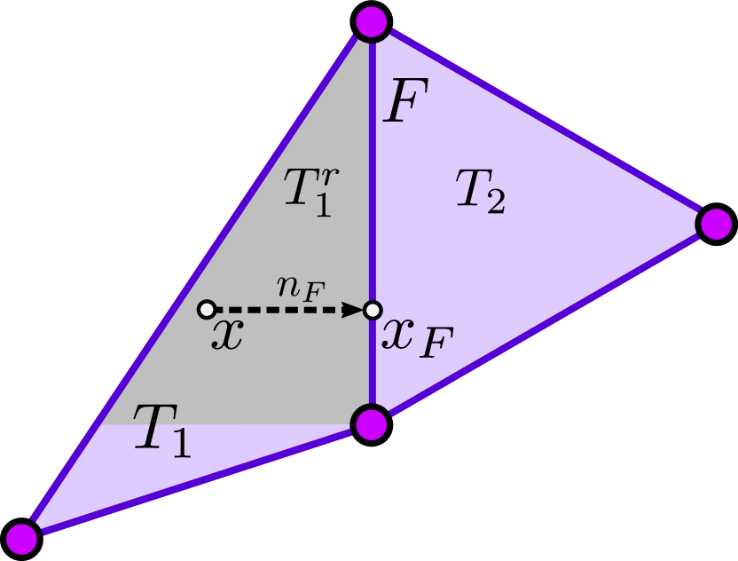
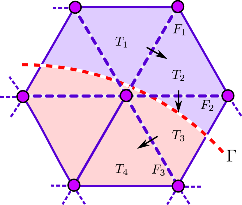
Figure 2.3: Controlling the $L^{2}$-norm $\|v\|_{T_{1}}$ of a finite element function $v$ on a barely intersected, “fictitious” element $T_{0}$ by $\|v\|_{T_{4}}$ and boundary zone jump-penalties. Starting from $T_{0}$, each term $\|v\|_{T_{i}}^{2}$ can be estimated by the neighboring term $\|v\|_{T_{i+1}^{2}}$ when a sum of jump-terms of the form $h_{F_{i+1}}^{2j+i}\|\dfrac{\partial}{\partial n}v\|_{F_{i+1}}^{2}$ is added.

As a first step, we recall from [104] how the local $L^{2}$ control of $v\in V_{h}$ can be passed between elements by adding a penalty of the jumps of all higher order normal derivatives.

Lemma 2.18

Let $T_{1},\,T_{2}\in\mathcal{T}_{h}$ be two elements sharing a common face $F$. Then for $v_{h}\in V_{h}$ the inequality

$$\|v\|_{T_{1}}^{2}\lesssim\|v\|_{T_{2}}^{2}+\sum_{0\leqslant j\leqslant k}h^{2j+1}([{\partial}_{n}^{j}v],[{\partial}_{n}^{j}v])_{F}$$ (2.82)

holds with the hidden constant depending only on the shape-regularity of $\mathcal{T}_{h}$, the polynomial order $k$, and the dimension d. Here, we used the notation ${\partial}_{n}^{j}v\coloneqq\sum_{|\alpha|=j}\tfrac{D^{\alpha}v(x)n^{\alpha}}{\alpha!}$ for multi-index $\alpha=(\alpha_{1},\ldots,\alpha_{d})$, $|\alpha|=\sum_{i}\alpha_{i}$ and $n^{\alpha}=n_{1}^{\alpha_{1}}n_{2}^{\alpha_{2}}\cdots n_{d}^{\alpha_{d}}$.

For the reader’s convenience, we include a slightly improved version of the proof from [104].

Proof 7

Let $n_{F}$ be the inward pointing face normal vector associated with $F$. For a given point $x\in T_{1}$, we write $x_{F}=x_{F}(x)$ for the normal projection of $x$ onto the plane defined by the face $F$. We define the set

$$T_{1}^{r}=\{x\in T_{1}\;|\;x_{F}+t(x-x_{F})\in T_{1}\;\forall\,t\in[0,1]\},$$ (2.83)

see also Figure 2.3 (left). By shape regularity and a finite dimension argument, there is a constant $C_{1}$ such that

$$\|v\|_{T_{1}}\leqslant C_{1}\|v\|_{T_{1}^{r}}.$$ (2.84)

Denote by $v_{i}$ the uniquely and globally defined polynomial satisfying $v_{i}|_{T_{i}}=v|_{T_{i}}$. For $i=1,2$ and $x\in T_{1}^{r}$, we may express $v_{i}(x)$ in terms of its Taylor expansion around $x_{F}$,

$$v_{i}(x)=\sum_{|\alpha|\leqslant k}\dfrac{D^{\alpha}v_{i}(x_{F})}{\alpha!}(|x-x_{F}|n)^{\alpha},$$ (2.85)

and subtracting the two Taylor expansions, we find that

$$v_{1}(x) =v_{2}(x)+\sum_{|\alpha|\leqslant k}\dfrac{[D^{\alpha}v(x_{F})n^{\alpha}]}{\alpha!}|x-x_{F}|^{\alpha}=v_{2}(x)+\sum_{j=0}^{k}|x-x_{F}|^{j}[{\partial}_{n}^{j}v(x_{F})].$$ (2.86)

After taking squares of the identity (2.86), multiple applications of a Cauchy-Schwarz inequality of the form $(\sum_{i}a_{i}b_{i})^{2}\leqslant\sum a_{i}^{2}\sum_{i}b_{i}^{2}$ show that

$$v_{1}^{2}(x)\leqslant 2v_{2}^{2}(x)+2(k+1)\sum_{j=0}^{k}|x-x_{F}|^{2j}[{\partial}_{n}^{j}v(x_{F})]^{2}.$$ (2.87)

Now, we integrate (2.87) over $T_{1}^{r}$ with respect to $x$ and exploit the fact that $x_{F}(x)$ is constant when integrating in face normal direction. With the height of $T_{1}^{r}$ over $F$ being bounded by $h$, we thus find that

$$C_{1}^{-1}\|v_{1}\|_{T_{1}}^{2} \leqslant\|v_{1}\|_{T_{1}^{r}}^{2}\leqslant 2\|v_{2}\|_{T_{1}^{r}}^{2}+2(k+1)\sum_{j=0}^{k}h^{2j}\int_{T_{1}^{r}}|[{\partial}_{n}^{j}v(x_{F}(x)]|^{2}\,\mathrm{d}x$$ (2.88)

$$\leqslant 2\|v_{2}\|_{T_{1}^{r}}^{2}+2(k+1)\sum_{j=0}^{k}h^{2j+1}\int_{F}|[{\partial}_{n}^{j}v(x_{F})]|^{2}\,\mathrm{d}x_{F},$$ (2.89)

$$\leqslant 2\max\{C_{2},k+1\}\bigg{(}\|v_{2}\|_{T_{2}}^{2}+\sum_{j=0}^{k}h^{2j+1}\|[{\partial}_{n}^{j}v]\|_{F}^{2}\biggr{)},$$ (2.90)

where in the last step, we again used the fact that the inequality $\|v_{2}\|_{T_{1}^{r}}\leqslant C_{2}\|v_{2}\|_{T_{2}}$ holds with some constant $C_{2}$ which only depends on the shape regularity parameter, the dimension $d$ and the order $k$.

The previous lemma is the main motivation to introduce the set of ghost penalty faces

$$\mathcal{F}_{h}^{g}=\{F\in\mathcal{F}_{h}:T^{+}\cap\Gamma\neq\emptyset\lor T^{-}\cap\Gamma\neq\emptyset\},$$ (2.91)

that is, the set of interior faces in active mesh belonging to elements which are intersected by the boundary $\Gamma$. See also Figure 2.1 (right), where the of ghost penalty faces are represented by dashed lines. Thanks to the geometric assumptions G2 and G3, we deduce that there is a uniformly bounded maximal number of ghost penalty faces which have to be crossed to “walk” from any element $T\in\mathcal{T}_{\Gamma}$ to an element $T^{\prime}$ satisfying the fat intersection property (2.14), see also Figure 2.3 (right). Thus we have derived the first estimate of the following lemma.

Lemma 2.19

For $v\in V_{h}$, it holds that

$$\|v\|_{\mathcal{T}_{h}}^{2}\lesssim\|v\|_{\Omega}^{2}+\sum_{j=0}^{k}\sum_{F\in\mathcal{F}_{h}^{g}}h^{2j+1}([{\partial}_{n}^{j}v],[{\partial}_{n}^{j}v])_{F},$$ (2.92)

$$\|\nabla v\|_{\mathcal{T}_{h}}^{2}\lesssim\|\nabla v\|_{\Omega}^{2}+\sum_{j=0}^{k}\sum_{F\in\mathcal{F}_{h}^{g}}h^{2j-1}([{\partial}_{n}^{j}v],[{\partial}_{n}^{j}v])_{F},$$ (2.93)

with the hidden constant only depending on the polynomial order $k$, the quasi-uniformity of $\mathcal{T}_{h}$ and the dimension $d$, but not on the particular cut configuration.

Proof 8

It only remains to show the second inequality. The prove (2.93), simply replace $v$ by $\nabla v$ in (2.92) in a first step, yielding

$$\|\nabla v\|_{\mathcal{T}_{h}}^{2}\lesssim\|\nabla v\|_{\Omega}^{2}+\sum_{j=0}^{k}\sum_{F\in\mathcal{F}_{h}^{g}}h^{2j+1}([\nabla{\partial}_{n}^{j}v],[\nabla{\partial}_{n}^{j}v])_{F}.$$ (2.94)

In the second step, decompose $\nabla v=(\partial_{n}v)n_{F}+{P}_{F}\nabla v$ into its facet normal and face tangential part using the tangential projection ${P}_{F}:=I-n_{F}\otimes n_{F}$ and then employ the inverse estimate

$$\|[P_{F}\nabla{\partial}_{n}^{j}v]\|_{F}^{2}=\|P_{F}\nabla[{\partial}_{n}^{j}v]\|_{F}^{2}\lesssim h^{-2}\|[{\partial}_{n}^{j}v]\|_{F}^{2}$$ (2.95)

on the tangential part to show that on each face $F$, we have

$$h^{2j+1}\|[{\partial}_{n}^{j}\nabla v]\|_{F}^{2}\lesssim h^{2j+1}\|[{\partial}_{n}^{j+1}v]\|_{F}^{2}+h^{2j-1}\|[{\partial}_{n}^{j}v]\|_{F}^{2}.$$ (2.96)

which establishes estimate (2.93).

Proposition 2.20

For any set of positive parameters $\{\gamma_{j}\}_{j=0}^{k}$, the ghost penalty $g^{1}_{h}$ defined by

$$g_{h}^{1}(v,w) \coloneqq\sum_{j=0}^{k}\sum_{F\in F_{h}^{g}}\gamma_{j}h_{F}^{2j-1}([{\partial}_{n}^{j}v],[{\partial}_{n}^{j}w])_{F},$$ (2.97)

for $v,w\in V_{h}$ satisfies Assumption EP1–EP4.

Remark 2.21

From a theoretical perspective, any pair of parameters choices $\{\gamma_{j}\}_{j=0}^{k}$ leads to equivalent discrete norms and thus we simply assume that $\gamma_{0}=\ldots=\gamma_{k}=1$ in all relevant proofs presented in this work. From a practical perspective, the choice of $\{\gamma_{j}\}_{j=0}^{k}$ will clearly affect the final constants in the derived estimates and consequently, the numerically observed robustness and accuracy of the method. In all our conducted numerical experiments, we chose $\beta=\gamma_{0}=50$ and $\gamma_{i}=0.1$ for $i=1,2,3$ as a good compromise between accuracy, robustness and conditioning.

Proof 9 (Proposition 2.20)

Thanks to Lemma 2.19, $g_{h}^{1}$ has both the $H^{1}$ and $L^{2}$ norm extension property and it only remains to show that EP2 and EP4 are satisfied. Starting with the weak consistency estimate (2.46), we let $v\in H^{s}(\Omega)$ and set $r=\min\{s,k+1\}$. Then

$$|\pi_{h}^{e}v|_{g_{h}^{1}}^{2} =\sum_{j=0}^{k}h^{2j-1}\|[{\partial}_{n}^{j}\pi_{h}^{e}v]\|_{\mathcal{F}_{h}^{g}}^{2}$$ (2.98)

$$=\sum_{j=0}^{r-1}h^{2j-1}\|[{\partial}_{n}^{j}(\pi_{h}^{e}v-v^{e})]\|_{\mathcal{F}_{h}^{g}}^{2}+\sum_{j=r}^{k}h^{2j-1}\|[{\partial}_{n}^{j}\pi_{h}^{e}v]\|_{\mathcal{F}_{h}^{g}}^{2}$$ (2.99)

$$\lesssim h^{2r-2}\|v\|_{r,\Omega}^{2}+h^{2j-2}\|D^{r}\pi_{h}^{e}v\|_{\mathcal{T}_{h}}^{2}$$ (2.100)

$$\lesssim h^{2r-2}\|v\|_{r,\Omega}^{2}.$$ (2.101)

where we combined the fact that $[{\partial}_{n}^{j}v^{e}]|_{F}=0$ for $0\leqslant j\leqslant r-1$ and the approximation property (2.41) to estimate the first sum appearing in (2.99). The second sum in (2.99) was treated by successively employing an inverse inequality of the form

$$\|\partial_{n}^{j}v\|_{F}\lesssim h^{r-j-\nicefrac{{1}}{{2}}}\|D^{r}v\|_{T},\quad v\in V_{h},$$ (2.102)

and the stability of the projection operator $\pi_{h}$ and the Sobolev extension operator in the $H^{r}$ norm. Finally, to establish the inverse estimate (2.99), simply use (2.102) with $r=0$.

Remark 2.22

The previous proof shows that if $v\in H^{k+1}(\Omega)$, the ghost penalty $g_{h}^{1}$ is in fact consistent since then $|v^{e}|_{g_{h}^{1}}=0$.

Remark 2.23

A closer inspection of the proofs of Lemma 2.19 and Proposition 2.20 reveals that for $v\in\mathbb{P}_{1}(\mathcal{T}_{h})$, the ghost penalty

$$\widetilde{g}_{h}^{1}(v,w)=\sum_{F\in\mathcal{F}_{h}^{g}}h([\nabla v],[\nabla w])_{F},$$ (2.103)

penalizing the full gradient jump satisfies all required assumptions except the $L^{2}$ extension property EP3. As a consequence, we would obtain geometrically robust a priori estimates but not robust condition number bounds when using $\widetilde{g}_{h}^{1}$, see also Remark 2.12 and 2.17.

2.7.2 Projection-based ghost penalties

To avoid the inconvenient evaluation of higher order normal derivatives appearing in the ghost penalty defined by (2.97) for polynomial order $k>1$, Burman [37] and Burman and Hansbo [44] proposed ghost penalty based on local projections, which we briefly review here in the context of cut discontinuous Galerkin methods. Let $P$ be a patch of $\operatorname{diam}(P)\lesssim h$ containing the two elements $T_{1}$ and $T_{2}$ and define the projection $\pi_{P}:L^{2}(P)\to\mathbb{P}_{k}(P)$ to be the $L^{2}$ projection onto the space of polynomials of order $k$ defined on the patch $P$. Then the next lemma first stated and proven in [37] shows that the $L^{2}$ norm of $v\in V_{h}$ can be passed from $T_{1}$ to $T_{2}$ by penalizing the deviation of $v|_{P}$ from its $L^{2}$ projection $\pi_{\mathcal{P}}v\in\mathbb{P}_{k}(P)$.

Lemma 2.24

Let $T_{1},T_{2}\in P$ and $\operatorname{diam}(P)\lesssim h$. Then for $v\in V_{h}$ its holds that

$$\|v\|_{T_{1}}^{2} \lesssim\|v\|_{T_{2}}^{2}+\|v-\pi_{P}v\|_{P}^{2},$$ (2.104)

$$\|\nabla v\|_{T_{1}}^{2} \lesssim\|\nabla v\|_{T_{2}}^{2}+h^{-2}\|v-\pi_{P}v\|_{P}^{2},$$ (2.105)

with the hidden constant only depending on the shape regularity of $\mathcal{T}_{h}$ the polynomials order $k$ and the dimension $d$.

Proof 10

For a proof we refer to Burman [37].

The previous lemma motivates the definition of a patch-wise local projection stabilization $g_{P}$ and its corresponding (global) ghost penalty $g_{h}^{2}$ by setting

$$g_{P}(v,w)=h^{-2}(v-\pi_{P}v,w-\pi_{P}w)_{P},\qquad g_{h}^{2}(v,w)=\sum_{P\in\mathcal{P}}g_{P}(v,w),$$ (2.106)

with $v,w\in V_{h}$. By choosing a suitable collections of patches $\mathcal{P}=\{P\}$, the previous lemma can now be applied in a number of ways to define ghost penalties for the cutDG formulation (2.13). For instance, a local projection stabilized analogue to the jump penalty based stabilization $g_{h}^{1}$ can be obtained by defining the patch $P(F)=T^{+}\cup T^{-}$ for two elements $T^{+}$, $T^{-}$ sharing the (interior) face $F$ and setting

$$\mathcal{P}_{1}=\{P(F)\}_{F\in\mathcal{F}_{h}^{g}}.$$ (2.107)

A second possibility is to simply use neighborhood patches $\omega(T)$,

$$\mathcal{P}_{2}=\{\omega(T)\}_{T\in\mathcal{T}_{\Gamma}}.$$ (2.108)

Finally, one can mimic the cell agglomeration approach taken in classical unfitted discontinuous Galerkin approaches [73, 77, 76, 84] by associating to each cut element $T\in\mathcal{T}_{\Gamma}$ with a small intersection $|T\cap\Omega|_{d}\leqslant c_{s}h_{T}^{d}$ an element $T^{\prime}\in\omega(T)$ satisfying the fat intersection property $|T^{\prime}\cap\Omega|_{d}\geqslant c_{s}h_{T^{\prime}}^{d}$. Setting the “agglomerated patch” $P_{a}(T)$ to $P_{a}(T)=T\cup T^{\prime}$, a proper collection of patches is given by

$$\mathcal{P}_{3}=\{P_{a}(T)\;|\;T\in\mathcal{T}_{\Gamma}\wedge|T\cap\Omega|\leqslant c_{s}h_{T}^{d}\}.$$ (2.109)

Lemma 2.25

For $\mathcal{P}\in\{\mathcal{P}_{1},\mathcal{P}_{2},\mathcal{P}_{3}\}$, the resulting projection based ghost penalty $g_{h}^{2}$ satisfies Assumption EP1–EP4.

Proof 11

Assumption EP1 and EP3 are clearly satisfied thanks to Lemma 2.24 and the geometric assumption G3. The inverse inequality (2.71) clearly holds by the very definition of $g_{P}$, so we are left with verifying Assumption EP2. Again, for $v\in H^{s}(\Omega)$ set $r=\min\{s,k+1\}$. Thanks to the approximation and stability properties of $\pi_{h}^{e}$ and $\pi_{P}$, the term $|\pi_{h}^{e}v|_{g_{h}^{2}}^{2}$ can be bounded by

$$|\pi_{h}^{e}v|_{g_{h}^{2}}^{2} =h^{-2}\|\pi_{h}^{e}v-\pi_{P}\pi_{h}^{e}v\|_{\mathcal{P}}^{2}$$ (2.110)

$$\lesssim h^{-2}\Bigl{(}\|\pi_{h}^{e}v-v^{e}\|_{\mathcal{P}}^{2}+\|v^{e}-\pi_{P}v^{e}\|_{\mathcal{P}}^{2}+\|\pi_{P}v^{e}-\pi_{P}\pi_{h}^{e}v\|_{\mathcal{P}}^{2}\Bigr{)}$$ (2.111)

$$\lesssim h^{-2}\Bigl{(}h^{2r}\|v\|_{r,\Omega}^{2}+h^{2r}\|v\|_{r,\Omega}^{2}+\|v^{e}-\pi_{h}^{e}v\|_{\mathcal{P}}^{2}\Bigr{)}$$ (2.112)

$$\lesssim h^{2r-2}\|v\|_{r,\Omega}^{2},$$ (2.113)

where we also used the fact that the number of patch overlaps is uniformly bounded.

2.8 Numerical examples

This section is devoted to corroborate our theoretical analysis by a number of numerical experiments. First, a convergence rate study for various approximation orders is conducted. Afterwards, we take a closer look at how the choice of the stabilization parameters affects the geometrical robustness of the energy error and the condition number of the overall system matrix.

2.8.1 Convergence rate studies

As a first test case, we numerically solve the Poisson problem (2.1) posed on the flower-like domain

$$\Omega =\{(x,y)\in\mathbb{R}^{2}\;|\;\phi(x,y)<0\}\quad\text{with }\phi(x,y)=\sqrt{x^{2}+y^{2}}-r_{0}-r_{1}\cos(\operatorname{atan_{2}}(y,x)),$$ (2.114)

setting $r_{0}=0.6$ and $r_{1}=0.2$. The analytical reference solution given by

$$u(z,y)=\cos(2\pi x)\cos(2\pi y)+\sin(2\pi x)\sin(2\pi y).$$ (2.115)

Starting from an initial tesselation $\widetilde{\mathcal{T}}_{0}$ of the domain $\Omega_{0}=[-1.1,1.1]^{2}\supset\Omega$, we generate a sequence of meshes $\{\mathcal{T}_{k}\}_{k=0}^{4}$ with mesh size $h_{k}=2.2\cdot 2^{-3-k}$ by successively refining $\widetilde{\mathcal{T}}_{0}$ and extracting the resulting active background mesh. On each mesh $\mathcal{T}_{k}$, we compute the numerical solution $u_{k}^{p}\in\mathbb{P}_{p}(\mathcal{T}_{k})$ to (2.13) using the ghost penalty $g_{h}^{1}$ defined by (2.97) together with the parameter set $\beta=\gamma_{0}=50.0$ and $\gamma_{p}=0.1$ for $p=1,2,3$. Based on the manufactured solution $u$, the experimental order of convergence (EOC) is calculated by

$$\text{EOC}(k,p)=\dfrac{\log(E_{k-1}^{p}/E_{k}^{p})}{\log(h_{k-1}/h_{k})},$$

where $E_{k}^{p}=\|e_{k}^{p}\|=\|u-u_{k}^{p}\|$ denotes the error of the numerical approximation $u_{k}^{p}$ measured in a certain norm $\|\cdot\|$. In our convergence tests, we consider both the $\|\cdot\|_{H^{1}(\Omega)}$ and the $\|\cdot\|_{L^{2}(\Omega)}$ norm. For each polynomial order $p=1,2,3$, we plot the resulting errors against the corresponding mesh size $h_{k}$ in a $\log$-$\log$-plot which confirms the theoretically predicted convergence rates for both the $H^{1}$ and $L^{2}$ error, see Figure 2.4.

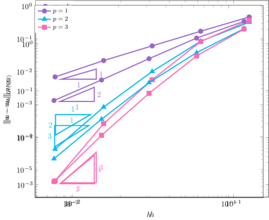
Figure 2.4: $H^{1}$ error (left) and $L^{2}$ error (right) convergence rates for the first, two-dimensional test case using different approximation orders $p=1,2,3$.

To demonstrate the applicability of our code to complex three-dimensional problems, we consider a second test case, where the model problem (2.1) is solved over a flower shaped, three-dimensional domain $\Omega=\{(x,y,z)\in\mathbb{R}^{3}\;|\;\phi(x,y,z)<0\}\subset\mathbb{R}^{3}$ defined by

$$\phi(x,y,z)=\sqrt{x^{2}+y^{2}+z^{2}}-r+(r/r_{0})\cos({5\operatorname{atan_{2}}(y,x)})\cos({\pi z}),$$

with $r=0.5$ and $r_{0}=3.5$. This time, we choose an analytic reference solution of the form

$$u(x,y,z)=\exp(x+y+z)\cos(x+y+z)\sin(x+y+z).$$ (2.116)

After embedding $\Omega$ into the domain $\Omega_{0}=[-0.8,0.8]^{3}$, a series of meshes $\{\mathcal{T}_{k}\}_{k=0}^{4}$ is generated with mesh size $h=1.6/N$, $N=6\cdot 2^{k}$ and the numerical solution is computed using $V_{h}=\mathbb{P}_{1}(\mathcal{T}_{k})$ and stabilization parameters $\beta=\gamma_{0}=50.0$, $\gamma_{1}=0.1$. The resulting EOC displayed in Table 2.1 corroborates the theoretical results from Section 2.5. Plots of the computed solutions to both the two- and three-dimensional test problems can be found in Figure 2.5.

$N_{k}$	$\|e_{k}^{1}\|_{H_{1}(\Omega)}$		EOC	$\|e_{k}^{1}\|_{L^{2}(\Omega)}$		EOC
$6$	$4.53$	$\cdot 10^{-1}$	–	$6.33$	$\cdot 10^{-2}$	–
$12$	$2.46$	$\cdot 10^{-1}$	$0.88$	$1.88$	$\cdot 10^{-2}$	$1.75$
$24$	$1.26$	$\cdot 10^{-1}$	$0.97$	$5.04$	$\cdot 10^{-3}$	$1.90$
$48$	$6.35$	$\cdot 10^{-2}$	$0.99$	$1.28$	$\cdot 10^{-3}$	$1.98$
$96$	$3.18$	$\cdot 10^{-2}$	$1.00$	$3.14$	$\cdot 10^{-4}$	$2.03$

Table 2.1: Convergence rates for three-dimensional test case using $\mathbb{P}_{1}(\mathcal{T}_{h})$.

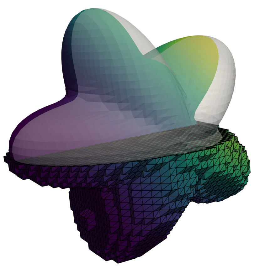
Figure 2.5: Solutions plots for the two-dimensional (left) and the three-dimensional (right) convergence study. The solutions are plotted over the active background mesh, together with actual the physical domain embedded into it. For the two-dimensional problem, the $\mathbb{P}_{2}(\mathcal{T}_{h})$ based solution is shown.

2.8.2 A numerical look at the $H^{1}$ extension property

Next, we illustrate numerically the role of the $H^{1}$ extension property defined in Assumption EP1. In a first experiment, we repeat the convergence study for the two-dimensional test problem from Section 2.8.1 using discontinuous $P_{1}$ elements and deactivate the ghost penalty by setting $\gamma_{0}=\gamma_{1}=0$. To trigger critical cut configurations more easily, we compute the corresponding numerical solutions on a series of non-hierarchical meshes $\{\mathcal{T}_{k}\}_{k=1}^{20}$ for the domain $[-0.8,0.8]^{2}$. More precisely, for $k=1,2,\ldots,20$, a structured mesh $\mathcal{T}_{k}$ was generated by subdividing each axis into $N=k\cdot 5$ subintervals and subsequently dividing each quadrilateral into two similar triangles. Figure 2.6 (left) displays the computed $H^{1}$ discretization error over the mesh size in a double logarithmic plot. The erratic convergence curve clearly illustrates that without properly defined ghost penalties, the particular cut configuration has a severe impact on the $H^{1}$ discretization error. On the contrary, the corresponding convergence curve for stabilized method with $\gamma_{0}=50$ and $\gamma_{1}=0.1$ has the theoretically expected slope. We repeat this experiment with alternative ghost penalty $\widetilde{g}_{h}^{1}(v,w)=\gamma_{1}h([\nabla v],[\nabla w])_{\mathcal{F}_{h}^{g}}$ satisfying only Assumption EP1, EP2, and EP4 (see Remark 2.23) and observe that the resulting convergence plot practically coincides with the one for the standard stabilized cutDGM. In all three cases, the $L^{2}$ convergence rate curve was practically unaffected by the particular cut configuration and thus was omitted from the convergence rate plots.

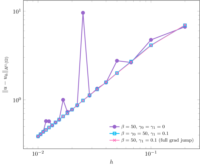
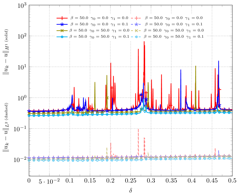
Figure 2.6: $H^{1}$ error cut configuration dependency studies. (Left) Convergence study for the two-dimensional test case on a series of non-hierarchical meshes using $\mathbb{P}_{1}(\mathcal{T}_{h})$ without ghost penalty, with ghost penalty $g_{h}^{1}$, and the alternative full grad jump ghost penalty $\widetilde{g}_{h}^{1}$. (Right) $H^{1}$ and $L^{2}$ error study on a single mesh computed for a family of gradually translated domains $\Omega_{1,\delta}$.

In a second experiment, we take a closer look at the influence of the cut configuration on the discretization error for a single fixed mesh. Again, we start from the two-dimensional test problem from Section 2.8.1 using discontinuous $P_{1}$ and define a $\mathcal{T}_{h}$. for $\Omega_{0}=[-0.8,0.8]^{2}$ with mesh size $h=1.6/8$. To create a large sample of possible cut configurations, we then generate a family of gradually translated domains $\{\Omega_{\delta_{k}}\}_{k=1}^{5000}$ where $\Omega_{\delta_{k}}=\Omega+\delta_{k}(h,h)$ with $\delta_{k}=k\cdot 2e^{-4}$ and the direction vector $(h,h)$. For each translated domain, we compute the $H^{1}$ and $L^{2}$ discretization error plot them as functions of $\delta_{k}$ in a semi-$\log$ plot, see Figure 2.6 (right). Again, the $H^{1}$ error for the fully activated ghost penalty $g_{h}^{1}$ with $\gamma_{0}=50$ and $\gamma_{1}=0.1$ is nearly completely unaffected by the cut configuration. When deactivating any of its contribution by either setting $\gamma_{0}$ or $\gamma_{1}$ (or both) to $0$, the $H^{1}$ error becomes clearly much more dependent on the particular cut configuration. In contrast, the $L^{2}$ error is nearly unaffected and shows only a few, less drastic spikes when the ghost penalty stabilization is turned off.

2.8.3 Condition number studies

We conclude the presentation of the numerical results with a series of experiments which illustrate the stabilizing effect of the ghost penalty on the condition number of the system matrix associated with the cutDGM (2.13). Following the experimental setup in Section 2.8.1, we now pick $\Omega_{1}=\{(x,y,z)\in\mathbb{R}^{3}\;|\;x^{2}+y^{2}+z^{2}-0.25^{2}\}$ which is embedded into the domain $[-0.51,0.51]^{3}$. The correspond family of translated domains $\{\Omega_{\delta_{k}}\}_{k=1}^{500}$ is defined through setting $\delta_{k}=k\cdot 0.002$. We also refer to Figure 2.7 for a principal sketch of the experimental setup.

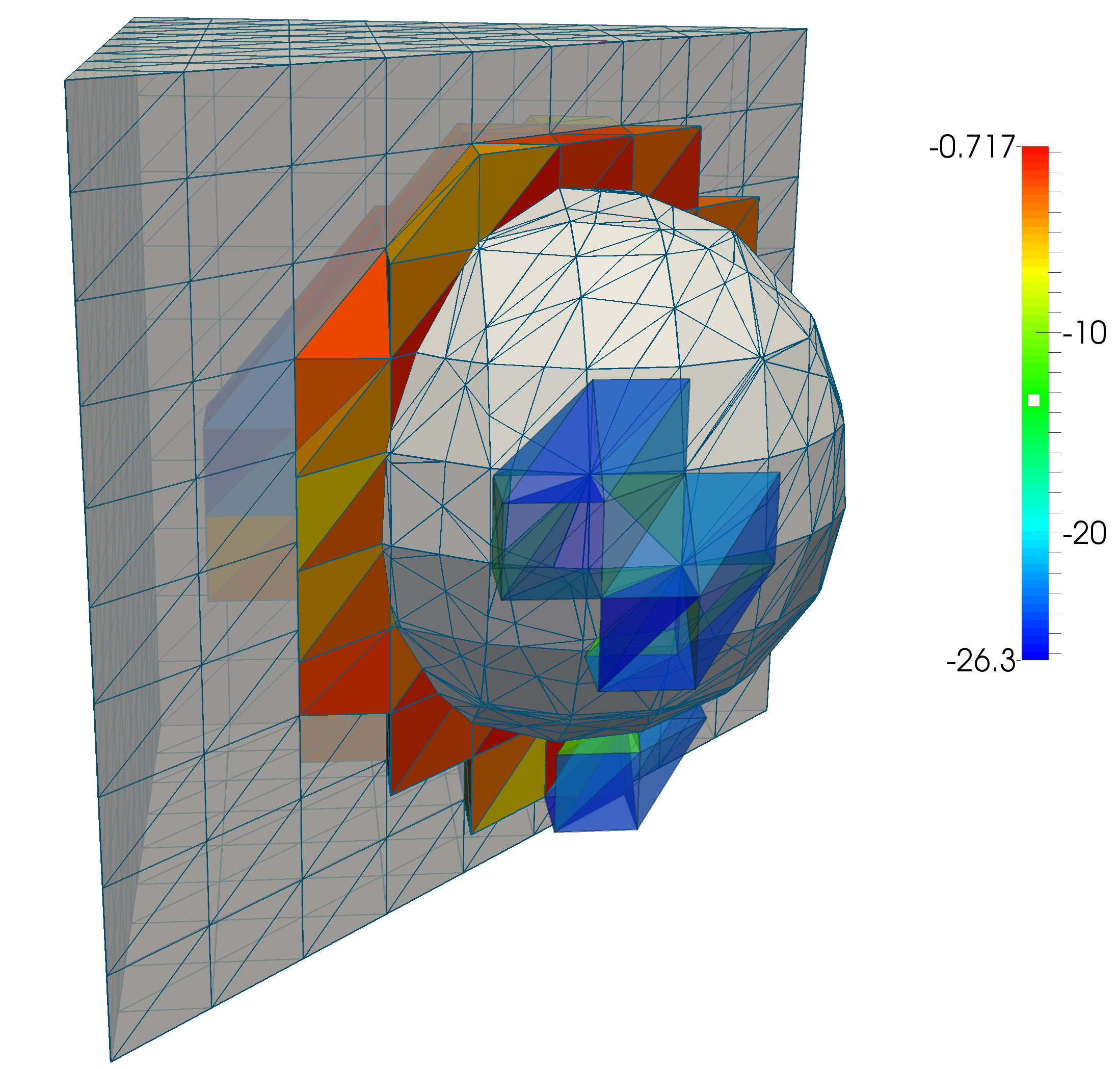
Figure 2.7: (Left) Principal experimental set-up to study the sensitivity of the conditon number with respect to the relative $\Gamma$ position. (Right): Snapshot of an intersection configuration when moving $\Gamma$ through the background mesh. To visualize “extreme” cut configurations, the color map plots for each intersected mesh element $T$ the value of $\log(\Gamma\cap T/\operatorname{diam}(T)^{2})$. Thus blue-colored elements contain only an extremely small fraction of the surface.

For each cut configuration, the condition number of system matrix associated with formulation (2.13) is computed and plotted against $\delta_{k}$ in a semi-$\log$ plot. We consider the fully activated ghost penalty $g_{h}^{1}$ with $\gamma_{0}=50$ and $\gamma_{1}=0.1$, partially deactivated versions of it and finally, the alternative ghost penalty $\widetilde{g}_{h}^{1}$ which does not satisfy the $L^{2}$ extension property EP3. As predicted by our theoretical analysis, the matrix condition number of all variants except for the fully activated ghost penalty $g_{h}^{1}$ is highly sensitive to the translation parameter $\delta$, see Figure 2.8 (left).

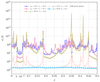
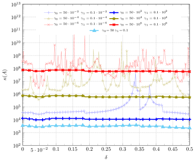
Figure 2.8: (Left) Condition number analysis for shifting domain with and without ghost penalty stabilization. (Right) Condition number analysis for changing values of stabilization parameters $\gamma_{0}$ and $\gamma_{1}$.

In a final numerical experiment, we assess the effect of the stability parameter magnitude on the magnitude and geometric robustness of the condition number. Starting from our standard parameter choice $\gamma_{0}=50$ and $\gamma_{1}=0.1$, we rescale the initial pair of parameters using rescaling factors ranging from $10^{-6}$ to $10^{6}$ and repeat the previous experiments. The resulting plot in Figure 2.8 (right) shows that both the base line magnitude and the fluctuation of the condition number decrease with increasing size of the stability parameters with a minimum around our parameter choice. A further increase of the stability parameters leaves the condition number insensitive to $\delta$, but leads to an increase of the overall magnitude. Combined with a series of convergence experiments (not presented here) for various parameter choices and combinations , we found that our standard parameter choice offers a good balance between the accuracy of the numerical scheme and the magnitude and fluctuation of the condition number.

3 Interface problems

In the final section, we demonstrate how the theoretical framework developed in Section 2.3–2.7, can be applied to formulate and analyze a cutDG method for interface problems. As before, we depart from a model problem and define suitable computational domains and approximation spaces leading us to a symmetric interior penalty based cutDG formulation. We present a short but complete theoretical analysis establishing geometrically robust error estimates in the energy norm, which are complemented with a number of convergence rate studies. For a detailed presentation and analysis of the corresponding cut finite element method for Poisson interface problems using continuous piecewise polynomials, we refer to [41, Section 3].

3.1 Model problem

Let $\Omega$ be a bounded, closed domain which is divided into two non-overlapping subdomains $\Omega_{1}$ and $\Omega_{2}$ by an interface $\Gamma=\partial\Omega_{1}\cap\partial\Omega_{2}$. Consider the Poisson interface problem

$$-\nabla\cdot(\kappa\nabla u) =f \quad\text{in }\Omega_{1}\cup\Omega_{2},$$ (3.1a)

$$u =g \quad\text{on }\partial\Omega,$$ (3.1b)

$$[u] =g_{D} \quad\text{on }\Gamma,$$ (3.1c)

$$[\kappa\partial_{n}u] =g_{N} \quad\text{on }\Gamma,$$ (3.1d)

where the restricted diffusion coefficient $\kappa_{i}=\kappa|_{\Omega_{i}}$ is supposed to be constant for $i=1,2$. Assuming the interface normal $n$ is pointing outward with respect to $\Omega_{1}$, the solution and normal flux jumps across $\Gamma$ are defined as usual by respectively

$$[u]=u_{1}|_{\Gamma}-u_{2}|_{\Gamma},\quad\text{and }\quad[\kappa\partial_{n}u]=\kappa_{1}\nabla u_{1}\cdot n-\kappa_{2}\nabla u_{2}\cdot n.$$ (3.2)

3.2 A cut discontinuous Galerkin method for the Poisson interface problem

As for the Poisson boundary problem, we assume that $\Omega$ is covered by a quasi-uniform background mesh $\widetilde{\mathcal{T}}_{h}$ with mesh size $h$. For each subdomain $\Omega_{i}$, $i=1,2$, the active background mesh $\mathcal{T}_{h,i}$ is again given by

$$\mathcal{T}_{h,i} =\{T\in{\mathcal{T}}_{h}:T\cap\Omega_{i}^{\circ}\neq\emptyset\}.$$ (3.3)

Finally, we denote the set of (interior and exterior) faces belonging to $\mathcal{T}_{h,i}$ by $\mathcal{F}_{h,i}$. Figure 3.1 illustrates the various computational domains and related mesh entities.

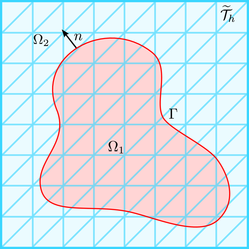
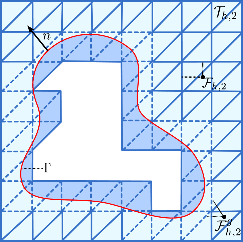
Figure 3.1: Computational domains for the interface problem. (Left) Original background mesh covering $\Omega=\Omega_{1}\cup\Omega_{2}$. (Middle) The active background mesh $\mathcal{T}_{h,1}$, internal faces $\mathcal{F}_{h,1}$ and the ghost penalty facets $\mathcal{F}_{h,1}^{g}$ associated with $\Omega_{1}$. (Right) Corresponding mesh entities associated with $\Omega_{2}$.

On the active mesh $\mathcal{T}_{h,i}$, we introduce the broken polynomial space of order $k$,

$$V_{h,i} =\mathbb{P}_{k}(\mathcal{T}_{h,i}),$$ (3.4)

and define the resulting total approximation space by

$$V_{h} =V_{h,1}\times V_{h,2}.$$ (3.5)

For $v=(v_{1},v_{2})\in V_{h}$, the weighted average of the normal flux along $\Gamma$ is given by

$$\{{\kappa\partial_{n}v}\}_{\omega} =\omega_{1}\kappa_{1}\partial_{n}v_{1}+\kappa_{2}\partial_{n}v_{2},$$ (3.6)

where the weights satisfy $0\leqslant\omega_{1},\omega_{2}\leqslant 1$ and $\omega_{1}+\omega_{2}=1$. In the following, we will also make use of the dual weighted average,

$$\langle{v}\rangle_{\omega} =\omega_{2}v_{1}+\omega_{1}v_{2}.$$ (3.7)

Moreover, unifying the notation for interior and exterior faces, we also set the jump and average operator on any exterior face $F$ belonging $\mathcal{T}_{h,i}$ to

$$\{{v}\}|_{F}=[v]|_{F}=v.$$ (3.8)

To write our cutDG formulation in a compact way and to facilitate the forthcoming numerical analysis, we introduce for $i=1,2$ the uncoupled, discrete bilinear forms

$$a_{h,i}(v_{i},w_{i}) =(\kappa_{i}\nabla v_{i},\nabla w_{i})_{\mathcal{T}_{h,i}\cap\Omega_{i}}-(\{{\kappa_{i}\partial_{n}v}\},[w])_{\mathcal{F}_{h,i}\cap\Omega_{i}}$$ (3.9)

$$\quad-([v],\{{\kappa_{i}\partial_{n}w}\})_{\mathcal{F}_{h,i}\cap\Omega_{i}}+\beta\kappa_{i}(h^{-1}[v],[w])_{\mathcal{F}_{h,i}\cap\Omega_{i}},$$ (3.10)

which involve only geometric quantities defined in the physical domain $\Omega_{i}$. The corresponding combined form is then

$$a_{h,\Omega}(v,w) =\sum_{i=1}^{2}a_{h,i}(v_{i},w_{i}),$$ (3.11)

and the coupling between the domains is encoded in the interface related bilinear form

$$a_{h,\Gamma}(v,w) =-(\{{\kappa_{i}\partial_{n}v}\}_{\omega},[w])_{\Gamma}-([v],\{{\kappa_{i}\partial_{n}w}\}_{\omega})_{\Gamma}+\beta_{\Gamma}(\kappa_{1},\kappa_{2})(h^{-1}[v],[w])_{\Gamma}.$$ (3.12)

To account for high contrast interface problems where the ratio $\tfrac{\kappa_{1}}{\kappa_{2}}$ can become arbitrary large or small, we employ harmonic weights following [105, 106, 41] and set the weights $\omega_{i}$ and the stability parameter $\beta_{\Gamma}$ to

$$\omega_{1}=\frac{\kappa_{2}}{\kappa_{1}+\kappa_{2}},\quad\omega_{2}=\frac{\kappa_{1}}{\kappa_{1}+\kappa_{2}},\quad\beta_{\Gamma}(\kappa_{1},\kappa_{2})=\widetilde{\beta}_{\Gamma}\dfrac{2\kappa_{1}\kappa_{2}}{\kappa_{1}+\kappa_{2}},$$ (3.13)

with $\widetilde{\beta}_{\Gamma}$ independent of $\kappa$. Alternative weights were proposed in  [107, 108], see also Remark 3.4. Next, similar to the cutDG formulation (2.13) for the Poisson boundary problem, we introduce ghost penalty enhanced versions of $a_{h,i}$ by setting

$$A_{h,i}(v_{i},w_{i}) =a_{h,i}(v_{i},w_{i})+g_{h,i}(v_{i},w_{i})\quad i=1,2,$$ (3.14)

and require that each $g_{h,i}$ individually satisfies the Assumption EP1–EP4 with respect to $\Omega_{i}$ and $\mathcal{T}_{h,i}$. Occasionally, we will also use the short-hand notation $g_{h}(v,w)=\sum_{i=1}^{2}g_{h,i}(v_{i},w_{i})$. Now the cutDG formulation for the interface problem (3.1) is to seek $u_{h}=(u_{h,1},u_{h,2})\in V_{h}$ such that

$$A_{h}(u_{h},v)\coloneqq\sum_{i=1}^{2}A_{h,i}(u_{h,i},v_{i})+a_{h,\Gamma}(u_{h},v)=l_{h}(v)\quad\forall\,v=(v_{1},v_{2})\in V_{h},$$ (3.15)

where the linear form $l_{h}$ is given by

$$l_{h}(v) =\sum_{i=1}^{2}(f_{i},v_{i})_{\mathcal{T}_{h,i}\cap\Omega_{i}}-(g_{D},\{{\kappa_{i}\partial_{n}v}\}_{\omega})_{\Gamma}+\beta_{\Gamma}(h^{-1}{g_{D}},[v])_{\Gamma}$$ (3.16)

$$\quad+(g_{N},\langle{v}\rangle_{\omega})_{\Gamma}-(g,\kappa_{2}\partial_{n}v)_{\partial\Omega}+\beta_{F,2}\kappa_{2}(h^{-1}g,v)_{\partial\Omega}.$$ (3.17)

3.3 Stability and convergence properties

As the theoretical investigation of the cutDG formulation of the Poisson interface problem will heavily rest upon the numerical analysis presented in Section 2, we decompose the energy norm for the final formulation (3.15) into domain specific and interface specific contributions. To this end, we define the discrete energy norms for $v_{i}\in V_{h,i}$, $i=1,2$ by

$$|\mspace{-1.0mu}|\mspace{-1.0mu}|v_{i}|\mspace{-1.0mu}|\mspace{-1.0mu}|_{a_{h,i}}^{2} =\|\nabla v_{i}\|^{2}_{\mathcal{T}_{h,i}\cap\Omega_{i}}+\|h^{-1/2}[v_{i}]\|^{2}_{\mathcal{F}_{h,i}\cap\Omega_{i}},$$ (3.18)

$$|\mspace{-1.0mu}|\mspace{-1.0mu}|v_{i}|\mspace{-1.0mu}|\mspace{-1.0mu}|^{2}_{A_{h,i}} =|\mspace{-1.0mu}|\mspace{-1.0mu}|v_{i}|\mspace{-1.0mu}|\mspace{-1.0mu}|^{2}_{a_{h,i}}+|v|^{2}_{g_{h,i}},$$ (3.19)

and the discrete energy norms associated with the total bilinear form $a_{h}$ and $A_{h}$ by

$$|\mspace{-1.0mu}|\mspace{-1.0mu}|v|\mspace{-1.0mu}|\mspace{-1.0mu}|^{2}_{a_{h}} =\sum_{i=1}^{2}|\mspace{-1.0mu}|\mspace{-1.0mu}|v_{i}|\mspace{-1.0mu}|\mspace{-1.0mu}|^{2}_{a_{h,i}}+\beta_{\Gamma}\|[h^{-1}v]\|_{\Gamma}^{2},$$ (3.20)

$$|\mspace{-1.0mu}|\mspace{-1.0mu}|v|\mspace{-1.0mu}|\mspace{-1.0mu}|^{2}_{A_{h}} =\sum_{i=1}^{2}|\mspace{-1.0mu}|\mspace{-1.0mu}|v_{i}|\mspace{-1.0mu}|\mspace{-1.0mu}|^{2}_{A_{h,i}}+\beta_{\Gamma}\|[h^{-1}v]\|_{\Gamma}^{2},$$ (3.21)

respectively. As an immediate result of the numerical analysis presented in Section 2.4, we record the following corollary, stating that the bulk forms $a_{h,i}$ are coercive with respect to $|\mspace{-1.0mu}|\mspace{-1.0mu}|\cdot|\mspace{-1.0mu}|\mspace{-1.0mu}|_{a_{h,i}}$.

Corollary 3.1

For $v=(v_{1},v_{2})\in V_{h}$, it holds that

$$|\mspace{-1.0mu}|\mspace{-1.0mu}|v_{i}|\mspace{-1.0mu}|\mspace{-1.0mu}|_{A_{h},i}^{2}\lesssim A_{h,i}(v_{i},v_{i})\quad i=1,2.$$ (3.22)

This observation allows us to give a short proof showing that the total discrete form $A_{h}$ defined by (3.15) is coercive in the discrete energy norm $|\mspace{-1.0mu}|\mspace{-1.0mu}|\cdot|\mspace{-1.0mu}|\mspace{-1.0mu}|_{A_{h}}$.

Proposition 3.2

It holds that

$$|\mspace{-1.0mu}|\mspace{-1.0mu}|v|\mspace{-1.0mu}|\mspace{-1.0mu}|_{A_{h}}^{2} \lesssim A_{h}(v,v) \quad\forall\,v\in V_{h}.$$ (3.23)

Proof 12

Since

$$A_{h}(v,v) =\sum_{i=1}^{2}A_{h,i}(v_{i},v_{i})+a_{h,\Gamma}(v,v)\gtrsim\sum_{i=1}^{2}|\mspace{-1.0mu}|\mspace{-1.0mu}|v_{i}|\mspace{-1.0mu}|\mspace{-1.0mu}|_{A_{h,i}}^{2}+a_{h,\Gamma}(v,v),$$ (3.24)

it only remains to treat the interface related contribution in (3.24). Recalling the definition of the weighted average $\{{\cdot}\}_{\omega}$, and successively applying an $\epsilon$-Young inequality and the trace estimate (2.70), we deduce that

$$2(\{{\kappa\partial_{n}v}\}_{\omega},[v])_{\Gamma} =2(\omega_{1}\kappa_{1}\partial_{n}v_{1}+\omega_{2}\kappa_{2}\partial_{n}v_{2},[v])_{\Gamma}$$ (3.25)

$$=\dfrac{2\kappa_{1}\kappa_{2}}{\kappa_{1}+\kappa_{2}}(\partial_{n}v_{1}+\partial_{n}v_{2},[v])_{\Gamma}$$ (3.26)

$$\lesssim\epsilon\dfrac{\kappa_{1}\kappa_{2}}{\kappa_{1}+\kappa_{2}}(\|h^{\nicefrac{{1}}{{2}}}\partial_{n}v_{1}\|_{\Gamma}^{2}+\|h^{\nicefrac{{1}}{{2}}}\partial_{n}v_{2}\|_{\Gamma}^{2})+\epsilon^{-1}\dfrac{2\kappa_{1}\kappa_{2}}{\kappa_{1}+\kappa_{2}}\|h^{-\nicefrac{{1}}{{2}}}[v]\|_{\Gamma}$$ (3.27)

$$\lesssim\epsilon\sum_{i=1}^{2}\kappa_{i}\|\nabla v_{i}\|_{\mathcal{T}_{h}}^{2}+\epsilon^{-1}\dfrac{2\kappa_{1}\kappa_{2}}{\kappa_{1}+\kappa_{2}}\|h^{-\nicefrac{{1}}{{2}}}[v]\|_{\Gamma}$$ (3.28)

$$\lesssim\epsilon\sum_{i=1}^{2}|\mspace{-1.0mu}|\mspace{-1.0mu}|v_{i}|\mspace{-1.0mu}|\mspace{-1.0mu}|_{A_{h,i}}^{2}+\epsilon^{-1}\dfrac{2\kappa_{1}\kappa_{2}}{\kappa_{1}+\kappa_{2}}\|h^{-\nicefrac{{1}}{{2}}}[v]\|_{\Gamma},$$ (3.29)

where in the last two steps, we used the fact that $\tfrac{\kappa_{1}\kappa_{2}}{\kappa_{1}+\kappa_{2}}\leqslant\min\{\kappa_{1},\kappa_{2}\}$ and the $H^{1}$ extension property of $g_{h,i}$. Now recalling that $\beta_{\Gamma}=\widetilde{\beta}_{\Gamma}\tfrac{2\kappa_{1}\kappa_{2}}{\kappa_{1}+\kappa_{2}}$, it follows that

$$a_{h,\Gamma}(v,v) =-2(\{{\kappa\partial_{n}v}\}_{\omega}[v])_{\Gamma}+\beta_{\Gamma}\|h^{-\nicefrac{{1}}{{2}}}[v]\|_{\Gamma}$$ (3.30)

$$\gtrsim-\epsilon\sum_{i=1}^{2}|\mspace{-1.0mu}|\mspace{-1.0mu}|v_{i}|\mspace{-1.0mu}|\mspace{-1.0mu}|_{A_{h,i}}^{2}+(\widetilde{\beta}_{\Gamma}-\epsilon^{-1})\dfrac{2\kappa_{1}\kappa_{2}}{\kappa_{1}+\kappa_{2}}\|h^{-\nicefrac{{1}}{{2}}}[v]\|_{\Gamma},$$ (3.31)

which together with (3.24) gives the desired result for $\epsilon$ small enough and $\widetilde{\beta}$ large enough.

Remark 3.3

The previous proof reveals that the key role of the ghost penalty forms $g_{h,i}$ is to extend the control of the domain-related energy norms $|\mspace{-1.0mu}|\mspace{-1.0mu}|\cdot|\mspace{-1.0mu}|\mspace{-1.0mu}|_{a_{h,i}}$ from physical subdomains $\Omega_{i}$ to the respective active meshes $\mathcal{T}_{h,i}$. As a consequence, we can closely follow the standard derivation of coercivity results for discontinuous Galerkin methods for high contrast interface and heterogeneous diffusion problems presented in [103, 41].

Remark 3.4

Barrau et al. [107] and Annavarapu et al. [108] proposed an unfitted Nitsche-based formulation for large contrast interface problems without ghost penalties using the weights

$$\omega_{1}=\dfrac{\kappa_{2}|T\cap\Omega_{1}|_{d}}{\kappa_{2}|T\cap\Omega_{1}|_{d}+\kappa_{1}|T\cap\Omega_{2}|_{d}},\qquad\omega_{2}=\dfrac{\kappa_{1}|T\cap\Omega_{2}|_{d}}{\kappa_{2}|T\cap\Omega_{1}|_{d}+\kappa_{1}|T\cap\Omega_{2}|_{d}},$$ (3.32)

and instead of $$\beta_{\Gamma}h^{-1}$$, a stability parameter of the form

$$\beta^{*}=\widetilde{\beta_{\Gamma}}\dfrac{\kappa_{1}\kappa_{2}|\Gamma\cap T|_{d-1}}{\kappa_{2}|T\cap\Omega_{1}|_{d}+\kappa_{1}|T\cap\Omega_{2}|_{d}}.$$ (3.33)

was employed. By incorporating the area of the physical element parts $T\cap\Omega_{i}$, this choice of weights accounts for both the contrast in the diffusion coefficient and the particular cut configuration. Consequently, this technique is not completely robust in the most extreme cases, where both a large contrast and a bad cut configuration must be handled simultaneously. For instance, let us consider again the sliver cut case in Figure 2.2 (left) with the normal $n$ pointing outwards with respect to $\Omega_{1}$. For a fixed mesh and mesh size, we see that if $\kappa_{2}\delta\geqslant\kappa_{1}h$ or equivalently, $\tfrac{\kappa_{2}}{\kappa_{1}}\geqslant\tfrac{h}{\delta}$, the stability parameter scales like

$$\dfrac{\kappa_{1}\kappa_{2}|\Gamma\cap T|_{d-1}}{\kappa_{2}|T\cap\Omega_{1}|_{d}+\kappa_{1}|T\cap\Omega_{2}|_{d}}\sim\dfrac{\kappa_{1}\kappa_{2}h^{d-1}}{\kappa_{2}\delta h^{d-1}+\kappa_{1}h^{d}}\geqslant\dfrac{\kappa_{1}\kappa_{2}h^{d-1}}{2\kappa_{2}\delta h^{d-1}}=\dfrac{\kappa_{1}}{2\delta}$$ (3.34)

and thus it can become arbitrary large in case of large contrast and a bad cut configuration. Using ghost penalty enhanced (continuous or discontinuous) unfitted finite element methods on the other hand, the stability parameter $\beta_{\Gamma}h^{-1}$ scales like $\beta_{\Gamma}h^{-1}\sim\min\{\kappa_{1},\kappa_{2}\}h^{-1}$ and thus is not affected by a large diffusion parameter $\kappa_{2}\gg\kappa_{1}$ or a particular bad cut configuration with $\delta\ll h$.

Thanks to the discrete coercivity estimate (3.23), we can now follow the derivation in Section 2.5 to prove optimal and geometrically robust a priori error estimates. To do so, we first define a suitable interpolation operator similar as in Section 2.5 by setting

$$\pi_{h}^{e}u=(\pi_{h,1}u_{1}^{e},\pi_{h,2}u_{2}^{e})$$ (3.35)

where $\pi_{h,i}:L^{2}(\mathcal{T}_{h,i})\to V_{h,i}$ for $i=1,2$. Then we have the following result.

Theorem 3.5

Let $u=(u_{1},u_{2})\in H^{s}(\Omega_{1})\times H^{s}(\Omega_{2})$ be the solution to the interface problem (3.1) and let $u_{h}=(u_{h,1},u_{h,2})\in\mathbb{P}_{k}(\mathcal{T}_{h,1})\times\mathbb{P}_{k}(\mathcal{T}_{h,2})$ be the solution to the cut discontinuous Galerkin formulation (3.15). Setting $r=\min\{s,k+1\}$, it holds that

$$|\mspace{-1.0mu}|\mspace{-1.0mu}|u-u_{h}|\mspace{-1.0mu}|\mspace{-1.0mu}|_{a_{h}}\lesssim\sum_{i=1}^{2}\kappa_{1}^{\nicefrac{{1}}{{2}}}h^{r-1}\|u_{i}\|_{r,\Omega_{i}}.$$ (3.36)

Proof 13

Following closely the derivation of the a priori estimate (2.47), we only sketch the proof. As before, by decomposing $u-u_{h}=(u-\pi_{h}^{e}u)+(\pi_{h}^{e}u-u_{h})=e_{\pi}+e_{h}$, it is enough to focus on the discrete error $e_{h}$. Combining the discrete coercivity and the weak Galerkin orthogonality of $A_{h}$, we see that

$$|\mspace{-1.0mu}|\mspace{-1.0mu}|e_{h}|\mspace{-1.0mu}|\mspace{-1.0mu}|_{A_{h}}^{2} \lesssim\sum_{i=1}^{2}\bigl{(}a_{h,i}(e_{\pi,i},e_{h,i})+g_{h,i}(\pi^{e}_{h,i}u_{i},e_{h,i})\bigr{)}+a_{h,\Gamma}(e_{\pi,i},e_{h})$$ (3.37)

$$\lesssim\sum_{i=1}^{2}h^{r-1}\kappa_{i}^{\nicefrac{{1}}{{2}}}\|u\|_{r,\Omega}|\mspace{-1.0mu}|\mspace{-1.0mu}|e_{h,i}|\mspace{-1.0mu}|\mspace{-1.0mu}|_{A_{h,i}}+a_{h,\Gamma}(e_{\pi},e_{h}).$$ (3.38)

Unwinding the definition of $a_{h,\Gamma}$ and recalling that $\omega_{i}\kappa_{i}\partial_{n}v_{i}=\tfrac{\kappa_{1}\kappa_{2}}{\kappa_{1}+\kappa_{2}}\partial_{n}v_{i}$ and that $\tfrac{\kappa_{1}\kappa_{2}}{\kappa_{1}+\kappa_{2}}\leqslant\min\{\kappa_{1},\kappa_{2}\}$, the remaining interface term can be estimated as in Corollary 2.7,

$$a_{h,\Gamma}(e_{\pi},e_{h}) =-(\{{\kappa_{i}\partial_{n}e_{\pi}}\}_{\omega},[e_{h}])_{\Gamma}-([e_{\pi}],\{{\kappa_{i}\partial_{n}e_{h}}\}_{\omega})_{\Gamma}+\widetilde{\beta}_{\Gamma}\dfrac{2\kappa_{1}\kappa_{2}}{\kappa_{1}+\kappa_{2}}(h^{-1}[e_{\pi}],[e_{h}])_{\Gamma}$$ (3.39)

$$\lesssim\min\{\kappa_{1},\kappa_{2}\}h^{r-1}\|u\|_{r,\Omega_{1}\cup\Omega_{2}}\|e_{h}\|_{A_{h}}.$$ (3.40)

3.4 Numerical examples

We conclude this work by briefly presenting a number of convergence rates studies conducted for two and three-dimensional interface problems with various contrast ratios. Throughout the numerical studies, we employ as ghost penalty the analog of $g_{h}^{1}$ defined in (2.97) and set for $i=1,2$,

$$g_{h,i}(v,w) \coloneqq\sum_{j=0}^{k}\sum_{F\in F_{h,i}^{g}}\gamma_{j}h_{F}^{2j-1}([{\partial}_{n}^{j}v],[{\partial}_{n}^{j}w])_{F},$$ (3.41)

with the ghost penalty faces

$$\mathcal{F}_{h,i}^{g} =\{F=T^{+}\cap T^{-}\in\mathcal{F}_{h,i}\;|\;T^{+}\cap\Gamma\neq\emptyset\lor T^{-}\Gamma\neq\emptyset\}.$$ (3.42)

3.4.1 Convergence rate studies for 2D interface problems

Based on geometry for the two-dimensional test case presented in Section 2.8.1, we now consider the interface problem (3.1) where the domains $\Omega_{1}$ and $\Omega_{2}$ are given by

$$\Omega_{1} =\{(x,y)\in\mathbb{R}^{2}\;|\;\phi(x,y)<0\}\quad\text{with }\phi(x,y)=\sqrt{x^{2}+y^{2}}-r_{0}-r_{1}\cos(\operatorname{atan_{2}}(y,x)),$$ (3.43)

$$\Omega_{2} =[-1.1,1.1]^{2}\setminus\Omega_{1}.$$ (3.44)

As before, we set $r_{0}=0.6$ and $r_{1}=0.2$. In our convergence study, we consider two cases. First, we define the simplest possible interface problem and set $\kappa_{1}=\kappa_{2}=1$ and $g_{D}=g_{N}=0$. We construct a manufactured solution based on the smooth analytical reference solution

$$u_{i}(x,y)=\cos(2\pi x)\cos(2\pi y)+\sin(2\pi x)\sin(2\pi y)\quad i=1,2$$ (3.45)

and compute the right-hand side $f$ and the boundary data $g$ accordingly. In the second test case, a high contrast interface problem is considered, setting $\kappa_{1}=1$ and $\kappa_{2}=10^{6}$ and employing the analytical reference solutions

$$u_{1}(x,y) =\sin(\pi(x-y))\cos(\pi(x+y)),$$ (3.46)

$$u_{2}(x,y) =\frac{1}{\kappa_{1}}\sin(0.5\pi(x+y))\cos(0.5\pi(x+y)).$$ (3.47)

This time, the interface data $g_{D}$ and $g_{N}$ are non-trivial functions as the chosen combination of $u_{1}$ and $u_{2}$ results in discontinuities in both the solution and the normal flux across the interface.

Following the presentation in Section 2.8.1, we conduct a convergence study for both cases, employing $V_{h}^{p}=\mathbb{P}_{p}(\mathcal{T}_{h,1})\times\mathbb{P}_{p}(\mathcal{T}_{h,2})$ for $p=1,2,3$. The resulting convergence curves associated with the $\|\kappa^{\nicefrac{{1}}{{2}}}\nabla(\cdot)\|_{L^{2}(\Omega_{1}\cup\Omega_{2})}$ norm are plotted in Figure 3.2 (left) and have the predicted optimal slopes. We also plot the convergence curves for the error measured in the $\|\cdot\|_{L^{2}(\Omega_{1}\cup\Omega_{2})}$ norm in Figure 3.2 (right), also showing optimal convergence rates for the chosen examples.

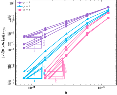
Figure 3.2: Convergence rate plots for the first (top) and second (bottom) two-dimensional test cases. Both the $\|\kappa^{\nicefrac{{1}}{{2}}}\nabla(\cdot)\|_{\Omega}$ (left) and $\|\cdot\|_{\Omega}$ (right) error plots show optimal convergence rates.

3.4.2 Convergence rate studies for 3D interface problems

In a final convergence study, we consider two test cases involving a three-dimensional interface problem posed in the domain $\Omega_{0}=[-1.1,1.1]^{3}$. For the first test problem, we define $\Omega_{1}$ as the union of $8$ balls $B_{r}(\boldsymbol{x}_{k})$ with $r=0.3$ and the $8$ center points $\boldsymbol{x}_{k}=(x_{k},y_{k},z_{k})$ given by $(\pm 0.5,\pm 0.5,\pm 0.5)$. Thus

$$\Omega_{1} =\{(x,y,z)\in\mathbb{R}^{3}\;|\;\phi(x,y,z)<1\},\quad\Omega_{2}=\Omega_{0}\setminus\Omega_{1},$$ (3.48)

with the level set function $\phi$ being defined by

$$\phi(x_{1},x_{2},x_{2})=\min_{0\leqslant k\leqslant 7}{\sqrt{(x-x_{k})^{2}+(y-y_{k})^{2}+(z-z_{k})^{2}}}-r.$$

We set $k_{1}=k_{2}=1$ and construct a manufactured solution from

$$u_{1}=u_{2}=\sin{(3\pi x)}+\sin{(3\pi y)}+\sin{(3\pi z)}\quad\mbox{ in }\Omega_{1}\cup\Omega_{2},$$ (3.49)

leading to a smooth solution and solution gradient across the interface $\Gamma$ and thus $g_{D}=g_{N}=0$.

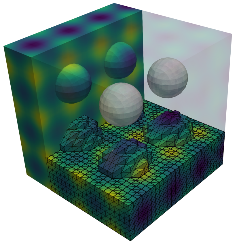
Figure 3.3: Solution plot for the first three-dimensional test case with no contrast and homogeneous jump conditions. The computed solution shows as expected a smooth transition across the interface.

In the second test case, we place $8$ balls of radius $r_{k}=0.8$, $k=0,\ldots 7$ at the $8$ corner points $(\pm 1,\pm 1,\pm 1)$ of $\Omega_{0}$ and add a cylinder with radius $r_{8}=0.6$ centered around $x$-axis. Using the standard notation $\delta_{ij}$ with $\delta_{ij}=1$ if $i=j$ and $0$ else, we can define the level set function $\phi$ and corresponding domains $\Omega_{1}$ and $\Omega_{2}$ by

$$\phi(x_{1},x_{2},x_{2})=\min_{0\leqslant k\leqslant 8}{\sqrt{(x-x_{k})^{2}\delta_{k8}+(y-y_{k})^{2}+(z-z_{k})^{2}}}-r_{k},$$ (3.50)

$$\Omega_{1}=\{(x,y,z)\in\Omega_{0}\;|\;\phi(x,y,z)<0\},\quad\Omega_{2}=\Omega_{0}\setminus\Omega_{1},$$ (3.51)

respectively. This time, we construct a manufactured solution with solution jumps and gradient jumps across the interface by setting

$$u_{1} =1/\kappa_{1}(\sin{(3\pi x)}+\sin{(3\pi y)}+\sin{(3\pi z)}),\quad \kappa_{1}=1 \quad\mbox{ in }\Omega_{1},$$ (3.52)

$$u_{2} =1/\kappa_{2}(\cos{(3\pi x)}+\cos{(3\pi y)}+\cos{(3\pi z)}),\quad \kappa_{2}=10 \quad\mbox{ in }\Omega_{2}.$$ (3.53)

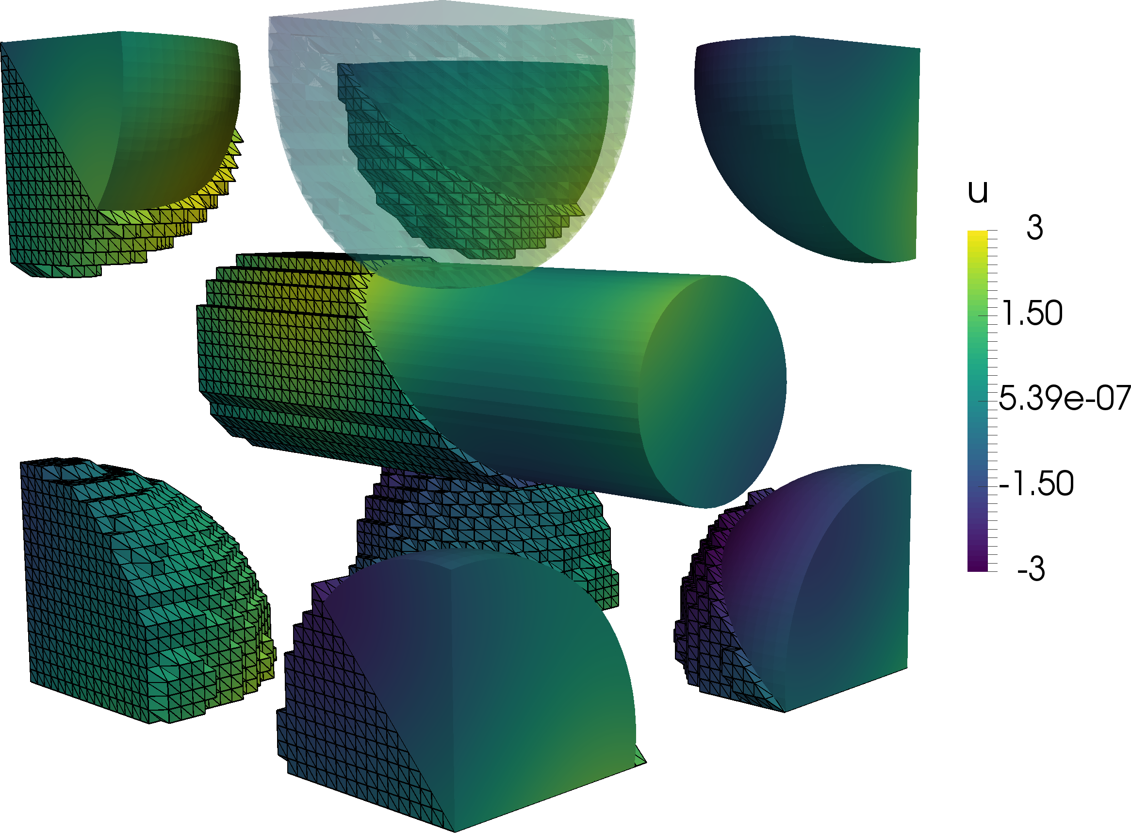
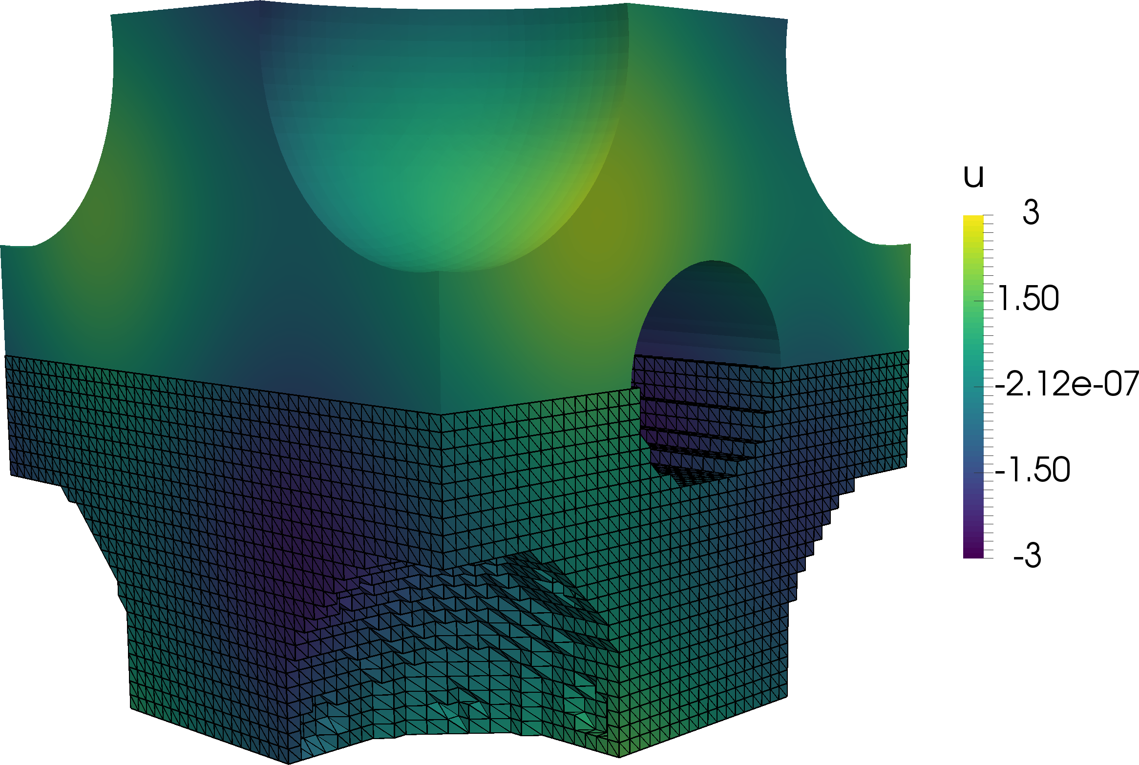
Figure 3.4: Solution plot for the second three-dimensional test case with a mild contrast and inhomogeneous jump conditions. The plots for $u_{1}$ (left) and $u_{2}$ (right) show the computed solution on parts of the physical domain as well as on its corresponding active mesh.

Focusing on piecewise linear approximations, we conduct a convergence study using $V_{h}=\mathbb{P}_{1}(\mathcal{T}_{h,1})\times\mathbb{P}_{1}(\mathcal{T}_{h,2})$ on a series of background meshes $\{\mathcal{T}_{k}\}_{k=1}^{7}$ with mesh size $h_{k}=2.2/N_{k}$ and $N_{k}\in\{6,9,12,18,24,36,48\}$. The computed EOC for both three-dimensional test cases are summarized in Table (3.1) and show optimal convergence with respect to the $\|\kappa^{\nicefrac{{1}}{{2}}}\nabla(\cdot)\|_{L^{2}(\Omega_{1}\cup\Omega_{2})}$ and $\|\cdot\|_{L^{2}(\Omega_{1}\cup\Omega_{2})}$ norm. Solution plots for the first and second test examples can be found in Figure 3.3 and 3.4.

$N_{k}$		$\|\kappa^{\nicefrac{{1}}{{2}}}\nabla e_{k}^{1}\|_{\Omega}$		EOC	$\|e_{k}^{1}\|_{\Omega}$		EOC		$\|\kappa^{\nicefrac{{1}}{{2}}}\nabla e_{k}^{1}\|_{\Omega}$		EOC	$\|e_{k}^{1}\|_{\Omega}$		EOC
$6$		$3.68$	$\cdot 10^{1}$	–	$4.20$	$\cdot 10^{0}$	–		$1.06$	$\cdot 10^{1}$	–	$6.93$	$\cdot 10^{-1}$	–
$9$		$2.51$	$\cdot 10^{1}$	$0.94$	$2.47$	$\cdot 10^{0}$	$1$	$.31$	$6.94$	$\cdot 10^{0}$	$1.04$	$3.46$	$\cdot 10^{-1}$	$1.71$
$12$		$1.98$	$\cdot 10^{1}$	$0.83$	$1.76$	$\cdot 10^{0}$	$1$	$.19$	$5.20$	$\cdot 10^{0}$	$1.01$	$1.96$	$\cdot 10^{-1}$	$1.97$
$18$		$1.29$	$\cdot 10^{1}$	$1.05$	$9.09$	$\cdot 10^{-1}$	$1$	$.62$	$3.44$	$\cdot 10^{0}$	$1.02$	$8.45$	$\cdot 10^{-2}$	$2.08$
$24$		$9.48$	$\cdot 10^{0}$	$1.08$	$5.24$	$\cdot 10^{-1}$	$1$	$.92$	$2.57$	$\cdot 10^{0}$	$1.01$	$4.66$	$\cdot 10^{-2}$	$2.07$
$36$		$6.20$	$\cdot 10^{0}$	$1.05$	$2.36$	$\cdot 10^{-1}$	$1$	$.97$	$1.73$	$\cdot 10^{0}$	$0.98$	$2.01$	$\cdot 10^{-2}$	$2.07$
$48$		$4.63$	$\cdot 10^{0}$	$1.02$	$1.32$	$\cdot 10^{-1}$	$2$	$.01$	$1.29$	$\cdot 10^{0}$	$1.02$	$1.11$	$\cdot 10^{-2}$	$2.06$

Table 3.1: Convergence rates for the first (left) and second (right) three-dimensional interface test problem using $\mathbb{P}_{1}(\mathcal{T}_{h})$.

References

- Allaire et al. [2014] G. Allaire, C. Dapogny, P. Frey, Shape optimization with a level set based mesh evolution method, Comput. Methods Appl. Mech. Engrg. 282 (2014) 22–53.
- Burman et al. [2018] E. Burman, D. Elfverson, P. Hansbo, M. G. Larson, K. Larsson, Shape optimization using the cut finite element method, Comput. Methods Appl. Mech. Engrg. 328 (2018) 242–261.
- Bernland et al. [2017] A. Bernland, E. Wadbro, M. Berggren, Acoustic shape optimization using cut finite elements, Int. J. Numer. Methods Eng. 113 (2017) 432–449.
- Tezduyar et al. [2006] T. E. Tezduyar, S. Sathe, R. Keedy, K. Stein, Space–time finite element techniques for computation of fluid–structure interactions, Comput. Methods Appl. Mech. Engrg. 195 (17) (2006) 2002–2027.
- MR and K. [1986] A. MR, O. K., Moving boundary-moving mesh analysis of phase change problems using finite elements and transfinite mappings, Int. J. Numer. Methods Eng. 23 (1986) 591–607.
- Groß et al. [2006] S. Groß, V. Reichelt, A. Reusken, A finite element based level set method for two-phase incompressible flows, Computing and Visualization in Science 9 (4) (2006) 239–257.
- Marchandise and Remacle [2006] E. Marchandise, J.-F. Remacle, A stabilized finite element method using a discontinuous level set approach for solving two phase incompressible flows, J. Comp. Phys. 219 (2) (2006) 780–800.
- Ganesan and Tobiska [2009] S. Ganesan, L. Tobiska, A coupled arbitrary Lagrangian–Eulerian and Lagrangian method for computation of free surface flows with insoluble surfactants, J. Comput. Phys. 228 (8) (2009) 2859–2873.
- Dassi et al. [2014] F. Dassi, S. Perotto, L. Formaggia, P. Ruffo, Efficient geometric reconstruction of complex geological structures, Math. Comput. Simul 106 (2014) 163–184.
- Antiga et al. [2009] L. Antiga, J. Peiró, D. A. Steinman, From image data to computational domains, in: Cardiovascular Mathematics, Springer, 123–175, 2009.
- Ural et al. [2011] A. Ural, P. Zioupos, D. Buchanan, D. Vashishth, The effect of strain rate on fracture toughness of human cortical bone: a finite element study, J. Mech. Behav. Biomed. Mater. 4 (7) (2011) 1021–1032.
- Cattaneo and Zunino [2014] L. Cattaneo, P. Zunino, Computational models for fluid exchange between microcirculation and tissue interstitium, Networks and Heterogeneous Media 9 (1).
- Dinh et al. [1992] Q. V. Dinh, R. Glowinski, J. He, V. Kwock, T. W. Pan, J. Periaux, Lagrange multiplier approach to fictitious domain methods: Application to fluid dynamics and electromagnetics, in: Fifth Int. Symp. Domain Decompos. Methods Partial Differ. Equations, T. Chan, D. Keyes, G. Meurant, J. Scroggs, R. Voigt, eds., Philadelphia, 151–194, 1992.
- Glowinski et al. [1994] R. Glowinski, T. Pan, J. Périaux, A fictitious domain method for Dirichlet problem and applications, Comput. Methods Appl. Mech. Engrg. 111 (1994) 283–303.
- Glowinski et al. [1995] R. Glowinski, T. Pan, J. Périaux, A Lagrange multiplier/fictitious domain method for Dirichlet problem. Generalization to some flow problems, Jpn. J. Ind. Appl. Math. 12 (1995) 87–108.
- Glowinski and Kuznetsov [2007] R. Glowinski, Y. Kuznetsov, Distributed Lagrange multipliers based on fictitious domain method for second order elliptic problems, Comput. Methods Appl. Mech. Engrg. 196 (8) (2007) 1498–1506.
- Glowinski et al. [1997] R. Glowinski, T. Pan, J. Periaux, A Lagrange multiplier/fictitious domain method for the numerical simulation of incompressible viscous flow around moving rigid bodies: (I) case where the rigid body motions are known a priori, Comptes Rendus l’Académie des Sci. - Ser. I - Math. 324 (3) (1997) 361–369.
- Glowinski et al. [1999a] R. Glowinski, T. W. Pan, J. Periaux, A distributed Lagrange multiplier/fictitious domain method for flows around moving rigid bodies: Application to particulate flow, Int. J. Numer. Meth. Fluids 30 (3) (1999a) 1043–1066.
- Glowinski et al. [1999b] R. Glowinski, T.-W. Pan, T. Hesla, D. Joseph, A distributed Lagrange multiplier/fictitious domain method for particulate flows, Int. J. Multiphase Flow 25 (5) (1999b) 755–794.
- Glowinski et al. [2001] R. Glowinski, T. Pan, T. Hesla, D. Joseph, J. Périaux, A fictitious domain approach to the direct numerical simulation of incompressible viscous flow past moving rigid bodies: application to particulate flow, J. Comp. Phys. 169 (2) (2001) 363–426.
- Moës et al. [1999] N. Moës, J. Dolbow, T. Belytschko, A finite element method for crack growth without remeshing, Int. J. Numer. Meth. Engng. 46 (1) (1999) 131–150.
- Melenk and Babuška [1996] J. Melenk, I. Babuška, The partition of unity finite element method: Basic theory and applications, Comput. Methods Appl. Mech. Engrg. 139 (1) (1996) 289–314.
- Chessa and Belytschko [2003] J. Chessa, T. Belytschko, An extended finite element method for two-phase fluids, J. Appl. Mech. 70 (1) (2003) 10–17.
- Zabaras et al. [2006] N. Zabaras, B. Ganapathysubramanian, L. Tan, Modelling dendritic solidification with melt convection using the extended finite element method, J. Comput. Phys. 218 (1) (2006) 200–227.
- Abbas et al. [2009] S. Abbas, A. Alizada, T. Fries, The XFEM for high-gradient solutions in convection-dominated problems, Int. J. Numer. Methods Eng. 82 (5) (2009) 1044–1072.
- Gerstenberger and Wall [2008] A. Gerstenberger, W. A. Wall, An extended finite element method/Lagrange multiplier based approach for fluid–structure interaction, Comput. Methods Appl. Mech. Engrg. 197 (19) (2008) 1699–1714.
- Fumagalli [2012] A. Fumagalli, Numerical modelling of flows in fractured porous media by the XFEM method, Ph.D. thesis, Italy, 2012.
- Fumagalli and Scotti [2014] A. Fumagalli, A. Scotti, An Efficient XFEM Approximation of Darcy Flows in Arbitrarily Fractured Porous Media, Oil & Gas Science and Technology–Revue d’IFP Energies nouvelles 69 (4) (2014) 555–564.
- Fries and Belytschko [2000] T.-P. Fries, T. Belytschko, The extended/generalized finite element method: An overview of the method and its applications, Int. J. Numer. Methods Eng. 00 (2000) 1–6.
- Hansbo and Hansbo [2002] A. Hansbo, P. Hansbo, An unfitted finite element method, based on Nitsche’s method, for elliptic interface problems, Comput. Methods Appl. Mech. Engrg. 191 (47-48) (2002) 5537–5552.
- Nitsche [1971] J. Nitsche, Über ein Variationsprinzip zur Lösung von Dirichlet-Problemen bei Verwendung von Teilräumen, die keinen Randbedingungen unterworfen sind, Abhandlungen aus dem Mathematischen Seminar der Universität Hamburg 36 (1) (1971) 9–15.
- Hansbo et al. [2003] A. Hansbo, P. Hansbo, M. G. Larson, A Finite Element Method on Composite Grids based on Nitsche’s Method, ESAIM: Math. Model. Numer. Anal. 37 (3) (2003) 495–514.
- Hansbo and Hansbo [2004] A. Hansbo, P. Hansbo, A finite element method for the simulation of strong and weak discontinuities in solid mechanics, Comput. Methods Appl. Mech. Engrg. 193 (33) (2004) 3523–3540.
- Areias and Belytschko [2006] P. M. Areias, T. Belytschko, A comment on the article “A finite element method for simulation of strong and weak discontinuities in solid mechanics” by A. Hansbo and P. Hansbo [Comput. Methods Appl. Mech. Engrg. 193 (2004) 3523–3540], Comput. Methods Appl. Mech. Engrg. 195 (9) (2006) 1275–1276.
- Becker et al. [2009] R. Becker, E. Burman, P. Hansbo, A Nitsche extended finite element method for incompressible elasticity with discontinuous modulus of elasticity, Comput. Methods Appl. Mech. Engrg. 198 (41-44) (2009) 3352–3360.
- Burman and Hansbo [2010] E. Burman, P. Hansbo, Fictitious domain finite element methods using cut elements: I. A stabilized Lagrange multiplier method, Comput. Methods Appl. Mech. Engrg. 199 (2010) 2680–2686.
- Burman [2010] E. Burman, Ghost penalty, C.R. Math. 348 (21-22) (2010) 1217–1220.
- Burman and Hansbo [2012] E. Burman, P. Hansbo, Fictitious domain finite element methods using cut elements: II. A stabilized Nitsche method, Appl. Numer. Math. 62 (4) (2012) 328–341.
- Burman et al. [2015a] E. Burman, S. Claus, P. Hansbo, M. G. Larson, A. Massing, CutFEM: discretizing geometry and partial differential equations, Internat. J. Numer. Meth. Engrg 104 (7) (2015a) 472–501.
- Bordas et al. [2018] S. Bordas, E. Burman, M. Larson, M. Olshanskii (Eds.), Geometrically Unfitted Finite Element Methods and Applications, Springer, 2018.
- Burman and Zunino [2012] E. Burman, P. Zunino, Numerical approximation of large contrast problems with the unfitted Nitsche method, Front. Numer. Anal. 2010 (2012) 1–54.
- Guzman et al. [2015] J. Guzman, M. A. Sanchez, M. Sarkis, A finite element method for high-contrast interface problems with error estimates independent of contrast, ArXiv e-prints .
- Burman et al. [2017] E. Burman, J. Guzmán, M. A. Sánchez, M. Sarkis, Robust flux error estimation of an unfitted Nitsche method for high-contrast interface problems, IMA J. Numer. Anal. .
- Burman and Hansbo [2014] E. Burman, P. Hansbo, Fictitious domain methods using cut elements: III. A stabilized Nitsche method for Stokes’ problem, ESAIM: Math. Model. Numer. Anal. 48 (3) (2014) 859–874.
- Massing et al. [2014a] A. Massing, M. G. Larson, A. Logg, M. E. Rognes, A stabilized Nitsche overlapping mesh method for the Stokes problem, Numer. Math. 128 (1) (2014a) 73–101.
- Burman et al. [2015b] E. Burman, S. Claus, A. Massing, A Stabilized Cut Finite Element Method for the Three Field Stokes Problem, SIAM J. Sci. Comput. 37 (4) (2015b) A1705–A1726.
- Cattaneo et al. [2014] L. Cattaneo, L. Formaggia, G. F. Iori, A. Scotti, P. Zunino, Stabilized extended finite elements for the approximation of saddle point problems with unfitted interfaces, Calcolo (2014) 1–30.
- Massing et al. [2018] A. Massing, B. Schott, W. Wall, A stabilized Nitsche cut finite element method for the Oseen problem, Comput. Methods Appl. Mech. Engrg. 328 (2018) 262–300.
- Winter et al. [2017] M. Winter, B. Schott, A. Massing, W. Wall, A Nitsche cut finite element method for the Oseen problem with general Navier boundary conditions, Comput. Methods Appl. Mech. Engrg. 330 (2017) 220–252.
- Kirchhart et al. [2016] M. Kirchhart, S. Groß, A. Reusken, Analysis of an XFEM discretization for Stokes interface problems, SIAM J. Sci. Comput. 38 (2) (2016) A1019–A1043.
- Groß et al. [2016] S. Groß, T. Ludescher, M. Olshanskii, A. Reusken, Robust preconditioning for XFEM applied to time-dependent Stokes problems, SIAM J. Sci. Comput. 38 (6) (2016) A3492–A3514.
- Guzmán and Olshanskii [2017] J. Guzmán, M. Olshanskii, Inf-sup stability of geometrically unfitted Stokes finite elements, To appear in Math. Comp. .
- Schott et al. [2015] B. Schott, U. Rasthofer, V. Gravemeier, W. A. Wall, A face-oriented stabilized Nitsche-type extended variational multiscale method for incompressible two-phase flow, Int. J. Numer. Methods Eng. 104 (7) (2015) 721–748.
- Groß and Reusken [2011] S. Groß, A. Reusken, Numerical methods for two-phase incompressible flows, vol. 40, Springer, 2011.
- Massing et al. [2015] A. Massing, M. G. Larson, A. Logg, M. Rognes, A Nitsche-based cut finite element method for a fluid-structure interaction problem, Commun. Appl. Math. Comput. Sci. 10 (2) (2015) 97–120.
- Olshanskii et al. [2009] M. A. Olshanskii, A. Reusken, J. Grande, A finite element method for elliptic equations on surfaces, SIAM J. Numer. Anal. 47 (5) (2009) 3339–3358.
- Olshanskii and Reusken [2010] M. A. Olshanskii, A. Reusken, A finite element method for surface PDEs: matrix properties, Numer. Math. 114 (3) (2010) 491–520.
- Burman et al. [2015c] E. Burman, P. Hansbo, M. G. Larson, A stabilized cut finite element method for partial differential equations on surfaces: The Laplace–Beltrami operator, Comput. Methods Appl. Mech. Engrg. 285 (2015c) 188–207.
- Burman et al. [2016a] E. Burman, P. Hansbo, M. G. Larson, A. Massing, Cut Finite Element Methods for Partial Differential Equations on Embedded Manifolds of Arbitrary Codimensions, ArXiv e-prints .
- Burman et al. [2016b] E. Burman, P. Hansbo, M. G. Larson, A. Massing, S. Zahedi, Full gradient stabilized cut finite element methods for surface partial differential equations, Comput. Methods Appl. Mech. Engrg. 310 (2016b) 278–296.
- Hansbo et al. [2017] P. Hansbo, M. Larson, A. Massing, A stabilized cut finite element method for the Darcy problem on surfaces, Comput. Methods Appl. Mech. Engrg. 326 (2017) 298–318.
- Grande et al. [2016] J. Grande, C. Lehrenfeld, A. Reusken, Analysis of a high order Trace Finite Element Method for PDEs on level set surfaces, ArXiv e-prints .
- Hansbo et al. [2016] P. Hansbo, M. G. Larson, S. Zahedi, A cut finite element method for coupled bulk-surface problems on time-dependent domains, Comput. Methods Appl. Mech. Engrg. 307 (2016) 96–116.
- Reusken [2014] A. Reusken, Analysis of trace finite element methods for surface partial differential equations, IMA J. Numer. Anal. 35 (2014) 1568–1590.
- Olshanskii and Reusken [2014] M. A. Olshanskii, A. Reusken, Error analysis of a space-time finite element method for solving PDEs on evolving surfaces, SIAM J. Numer. Anal. 52 (4) (2014) 2092–2120.
- Flemisch et al. [2016] B. Flemisch, A. Fumagalli, A. Scotti, A Review of the XFEM-Based Approximation of Flow in Fractured Porous Media, in: Advances in Discretization Methods: Discontinuities, Virtual Elements, Fictitious Domain Methods, vol. 12, Springer, 47–76, 2016.
- D’Angelo and Scotti [2012] C. D’Angelo, A. Scotti, A mixed finite element method for Darcy flow in fractured porous media with non-matching grids, ESAIM: Math. Model. Numer. Anal. 46 (02) (2012) 465–489.
- Formaggia et al. [2013] L. Formaggia, A. Fumagalli, A. Scotti, P. Ruffo, A reduced model for Darcy’s problem in networks of fractures, ESAIM: Math. Model. Numer. Anal. 48 (4) (2013) 1089–1116.
- Parvizian et al. [2007] J. Parvizian, A. Düster, E. Rank, Finite cell method, Comput. Mech. 41 (1) (2007) 121–133.
- Varduhn et al. [2016] V. Varduhn, M.-C. Hsu, M. Ruess, D. Schillinger, The tetrahedral finite cell method: Higher-order immersogeometric analysis on adaptive non-boundary-fitted meshes, Int. J. Numer. Meth. Engng. 107 (2016) 1054–1079.
- Xu et al. [2016] F. Xu, D. Schillinger, D. Kamensky, V. Varduhn, C. Wang, M.-C. Hsu, The tetrahedral finite cell method for fluids: Immersogeometric analysis of turbulent flow around complex geometries, Comput. Fluids 141 (2016) 135–154.
- Schillinger and Ruess [2014] D. Schillinger, M. Ruess, The finite cell method: A review in the context of higher-order structural analysis of cad and image-based geometric models, Arch. Comput. Methods Eng. (2014) 1–65.
- Bastian and Engwer [2009] P. Bastian, C. Engwer, An unfitted finite element method using discontinuous Galerkin, Internat. J. Numer. Meth. Engrg 79 (12) (2009) 1557–1576.
- Bastian et al. [2011] P. Bastian, C. Engwer, J. Fahlke, O. Ippisch, An Unfitted Discontinuous Galerkin method for pore-scale simulations of solute transport, Math. Comput. Simul 81 (10) (2011) 2051–2061.
- Saye [2015] R. I. Saye, High-Order Quadrature Methods for Implicitly Defined Surfaces and Volumes in Hyperrectangles, SIAM J. Sci. Comput. 37 (2) (2015) A993–A1019.
- Sollie et al. [2011] W. E. H. Sollie, O. Bokhove, J. J. W. van der Vegt, Space–time discontinuous Galerkin finite element method for two-fluid flows, J. Comput. Phys. 230 (3) (2011) 789–817.
- Heimann et al. [2013] F. Heimann, C. Engwer, O. Ippisch, P. Bastian, An unfitted interior penalty discontinuous Galerkin method for incompressible Navier–Stokes two–phase flow, Internat. J. Numer. Methods Fluids 71 (3) (2013) 269–293.
- Saye [2017] R. Saye, Implicit mesh discontinuous Galerkin methods and interfacial gauge methods for high-order accurate interface dynamics, with applications to surface tension dynamics, rigid body fluid-structure interaction, and free surface flow: Part I, J. Comput. Phys. 344 (2017) 647–682.
- Müller et al. [2016] B. Müller, S. Krämer-Eis, F. Kummer, M. Oberlack, A high-order Discontinuous Galerkin method for compressible flows with immersed boundaries, Int. J. Numer. Methods Eng. 110 (1) (2016) 3–30, nme.5343.
- Krause and Kummer [2017] D. Krause, F. Kummer, An Incompressible Immersed Boundary Solver for Moving Body Flows using a Cut Cell Discontinuous Galerkin Method, Comput. Fluids 153 (2017) 118–129.
- Badia et al. [2017] S. Badia, F. Verdugo, A. F. Martín, The aggregated unfitted finite element method for elliptic problems, arXiv preprint arXiv:1709.09122 .
- Badia and Verdugo [2017] S. Badia, F. Verdugo, Robust and scalable domain decomposition solvers for unfitted finite element methods, J. Comput. Appl. Math. .
- Massjung [2012] R. Massjung, An unfitted discontinuous Galerkin method applied to elliptic interface problems, SIAM J. Numer. Anal. 50 (6) (2012) 3134–3162.
- Johansson and Larson [2013] A. Johansson, M. Larson, A High Order Discontinuous Galerkin Nitsche Method for Elliptic Problems with Fictitious Boundary, Numer. Math. 123 (4).
- Antonietti et al. [2016a] P. F. Antonietti, A. Cangiani, J. Collis, Z. Dong, E. H. Georgoulis, S. Giani, P. Houston, Review of discontinuous Galerkin finite element methods for partial differential equations on complicated domains, in: Building Bridges: Connections and Challenges in Modern Approaches to Numerical Partial Differential Equations, Springer, 279–308, 2016a.
- Antonietti et al. [2016b] P. F. Antonietti, C. Facciola, A. Russo, M. Verani, Discontinuous Galerkin approximation of flows in fractured porous media on polytopic grids, Tech. Rep., MOX, Dipartimento di Matematica, Politecnico di Milano, 2016b.
- Giani and Houston [2014] S. Giani, P. Houston, Goal-oriented adaptive composite discontinuous Galerkin methods for incompressible flows, J. Comput. Appl. Math. 270 (2014) 32–42.
- Müller et al. [2013] B. Müller, F. Kummer, M. Oberlack, Highly accurate surface and volume integration on implicit domains by means of moment-fitting, Internat. J. Numer. Meth. Engrg 6 (2013) 10–16.
- Lehrenfeld [2016] C. Lehrenfeld, High order unfitted finite element methods on level set domains using isoparametric mappings, Comput. Methods Appl. Mech. Engrg. 300 (2016) 716–733.
- Fries and Omerović [2016] T.-P. Fries, S. Omerović, Higher-order accurate integration of implicit geometries, Int. J. Numer. Methods Eng. 106 (2016) 323–371.
- Fries et al. [2017] T. Fries, S. Omerović, D. Schöllhammer, J. Steidl, Higher-order meshing of implicit geometries—Part I: Integration and interpolation in cut elements, Comput. Methods Appl. Mech. Engrg. 313 (2017) 759–784.
- Gürkan and Massing [2018a] C. Gürkan, A. Massing, A stabilized cut discontinuous Galerkin framework: II. Hyperbolic and advection-dominated problems, Submitted. .
- Gürkan and Massing [2018b] C. Gürkan, A. Massing, A stabilized cut discontinuous Galerkin framework: III. Surface and mixed dimensional coupled problems, In preparation. .
- Burman et al. [2016a] E. Burman, P. Hansbo, M. G. Larson, A. Massing, A cut discontinuous Galerkin method for the Laplace–Beltrami operator, IMA J. Numer. Anal. 37 (1) (2016a) 138–169.
- Massing [2017] A. Massing, A Cut Discontinuous Galerkin Method for Coupled Bulk-Surface Problems, chap. Chapter in UCL Workshop volumen on ”Geometrically Unfitted Finite Element Methods”, to appear in Lecture Notes in Computational Science and Engineering, Springer, 1–19, 2017.
- Gilbarg and Trudinger [2001] D. Gilbarg, N. S. Trudinger, Elliptic Partial Differential Equations of Second Order, Classics in Mathematics, Springer-Verlag, Berlin, 2001.
- Li et al. [2010] J. Li, J. Melenk, B. Wohlmuth, J. Zou, Optimal a priori estimates for higher order finite elements for elliptic interface problems, Appl. Numer. Math. 60 (1) (2010) 19–37.
- Burman et al. [2016b] E. Burman, P. Hansbo, M. Larson, S. Zahedi, Cut Finite Element Methods for Coupled Bulk-Surface Problems, Numer. Math. 133 (2016b) 203–231.
- Groß et al. [2015] S. Groß, M. A. Olshanskii, A. Reusken, A trace finite element method for a class of coupled bulk-interface transport problems, ESAIM: Math. Model. Numer. Anal. 49 (5) (2015) 1303–1330.
- Stein [1970] E. Stein, Singular Integrals and Differentiability Properties of Functions, Princeton University Press, 1970.
- Ern and Guermond [2006] A. Ern, J.-L. Guermond, Evaluation of the condition number in linear systems arising in finite element approximations, ESAIM: Math. Model. Numer. Anal. 40 (1) (2006) 29–48.
- Arnold [1982] D. Arnold, An interior penalty finite element method with discontinuous elements, SIAM J. Num. Anal. 19 (4) (1982) 742–760.
- Di Pietro and Ern [2012] D. A. Di Pietro, A. Ern, Mathematical aspects of discontinuous Galerkin methods, vol. 69, Springer, 2012.
- Massing et al. [2014b] A. Massing, M. Larson, A. Logg, M. Rognes, A stabilized Nitsche fictitious domain method for the Stokes problem, J. Sci. Comput. 61 (3) (2014b) 604–628.
- Dryja [2003] M. Dryja, On discontinuous Galerkin methods for elliptic problems with discontinuous coefficients, Comput. Methods Appl. Math. 3 (1) (2003) 76–85.
- Ern et al. [2009] A. Ern, A. F. Stephansen, P. Zunino, A discontinuous Galerkin method with weighted averages for advection–diffusion equations with locally small and anisotropic diffusivity, IMA J. Numer. Anal. 29 (2009) 235–256.
- Barrau et al. [2012] N. Barrau, R. Becker, E. Dubach, R. Luce, A robust variant of NXFEM for the interface problem, C.R. Math. 350 (15) (2012) 789–792.
- Annavarapu et al. [2012] C. Annavarapu, M. Hautefeuille, J. E. Dolbow, A robust Nitsche’s formulation for interface problems, Comput. Methods Appl. Mech. Engrg. 225 (2012) 44–54.