A Deal with the Devil: From Divergent Perturbation Theory to an Exponentially-Convergent Self-Consistent Expansion

Abstract

For many nonlinear physical systems, approximate solutions are pursued by conventional perturbation theory in powers of the non-linear terms. Unfortunately, this often produces divergent asymptotic series, collectively dismissed by Abel as “an invention of the devil.” Although a lot of progress has been made on understanding the mathematics and physics behind this, new approaches are still called for. A related method, the self-consistent expansion (SCE), has been introduced by Schwartz and Edwards. Its basic idea is a rescaling of the zeroth-order system around which the solution is expanded, to achieve optimal results. While low-order SCEs have been remarkably successful in describing the dynamics of non-equilibrium many-body systems (e.g., the Kardar-Parisi-Zhang equation), its convergence properties have not been elucidated before. To address this issue we apply this technique to the canonical partition function of the classical harmonic oscillator with a quartic $gx^{4}$ anharmonicity, for which perturbation theory’s divergence is well-known. We obtain the $N$th order SCE for the partition function, which is rigorously found to converge exponentially fast in $N$, and uniformly in $g\geq 0$. We use our results to elucidate the relation between the SCE and the class of approaches based on the so-called “order-dependent mapping.” Moreover, we put the SCE to test against other methods that improve upon perturbation theory (Borel resummation, hyperasymptotics, Padé approximants, and the Lanczos $\tau$-method), and find that it compares favorably with all of them for small $g$ and dominates over them for large $g$. The SCE is shown to converge to the correct partition function for the double-well potential case, even when expanding around the local maximum. Our treatment is generalized to the case of many oscillators, as well as to any nonlinearity of the form $g|x|^{q}$ with $q\geq 0$ and complex $g$. These results allow us to treat the Airy function, and to see the fingerprints of Stokes lines in the SCE.

I Introduction

A recurring theme in physics is the necessity of approximations. Exactly solvable systems are rare in the landscape of modern science, and the majority of physical problems cannot be assailed directly without resorting to any estimates or simplifications. First-principle calculations must often be replaced by phenomenological models, which are then only solved approximately, to varying degrees of success. The ability to make informed, strategic approximations that would allow us to gain ground, but still capture the essential physics under consideration, is as much an art as it is a science. To this end, over the last centuries, practitioners of the natural sciences have collectively amassed an ever-expanding arsenal of indispensable techniques and methods in their professional toolbox.

Chief among these tools is the concept of perturbative expansion Boyd (1999). Its premise is simple and elegant: for a given difficult problem, identify a related but easier one; solve the simpler system exactly; and apply corrections to obtain an approximate solution to the original problem. This time-tested principle is applied at all hierarchies of engagement, from Taylor’s theorem to quantum field theory. Broadly speaking, linear systems, where the cumulative impact of additional intricacies is additive, are considered “simple,” while nonlinear systems are deemed “complicated.” An expansion of a nonlinear system about its linear counterpart, in powers the non-linearity, is recognized as a Perturbation Theory (PT).

Unfortunately, PT frequently produces an asymptotic, divergent expansion. While this in practice provides sensible answers when applied to low orders (quantum electrodynamics, for instance, is a remarkable example Feynman (1949)), in principle it denies us high-accuracy, large-order results, especially for strongly coupled systems. Over time, the non-perturbative physical processes which stand behind this behavior (tunneling, instantons, solitons, etc. Zinn-Justin (2002)) have been identified, which have also allowed for the development of sophisticated mathematical techniques for extracting correct physical results from PT. These efforts include resummation schemes, such as Borel Costin (2008), successive expansions of the PT remainder Berry and Howls (1990), methods based on the theory of resurgence Cherman et al. (2015); Aniceto et al. (2018), and various numerical and asymptotic prescriptions Bender and Orszag (1978); Boyd (1999). However, these are usually technically difficult to implement, especially to large order, and typically on a case-by-case basis. This situation was surmised by Abel, who begrudgingly proclaimed (Abel, , loosely translated) “divergent series are an invention of the devil, and it is shameful to base on them any demonstration whatsoever.” This implies an erroneous application of a perturbative approach in systems where the fundamental phenomena are non-perturbative. We stress that the issue is not the divergence of individual perturbative terms, which is usually tamed by other means (such as regularization and renormalization Peskin and Schroder (1995) for IR/UV catastrophes, and secular PT Strogatz (1994) for the time dependence of nonlinear systems at long times), but rather the divergence of the PT series itself, even if all its constituent terms are finite.

A related technique, the Self-Consistent Expansion (SCE) Schwartz and Katzav (2008); Cohen et al. (2016), was introduced by Schwartz and Edwards Schwartz and Edwards (1992, 1998) in their study of the Kardar–Parisi–Zhang (KPZ) problem of nonlinear deposition Kardar et al. (1986). The KPZ equation is not amenable to PT, as Wiese showed Wiese (1998) that above two dimensions, the KPZ strongly-coupled phase is inherently inaccessible by a perturbative expansion, regardless of its order. In contrast, the SCE, utilized at low orders, was remarkably successful in reproducing exact critical values in one dimension and agreeing with numerical values in higher dimensions. This method was subsequently applied to more complicated variants of the KPZ equation Katzav and Schwartz (1999); Schwartz and Edwards (2002); Katzav (2003); Katzav and Schwartz (2004a, b), and to other problems such as fracture, turbulence, and the XY model Katzav and Adda-Bedia (2006); Katzav et al. (2007); Edwards and Schwartz (2002); Li et al. (1996).

The SCE’s central idea is to smartly choose the zeroth-order system around which one expands, so that the zeroth-order system is as close as possible, in some sense, to the perturbed one. The SCE prescription is Schwartz and Katzav (2008); Cohen et al. (2016): (i) Decide on the order $N$ of the expansion. (ii) Split the potential into zeroth- and first-order terms parametrically as a function of $N$, namely

$$V\left(x\right)=V_{0}\left(x;N\right)+V_{1}\left(x;N\right)\,.$$ (1)

Fix this partitioning by demanding some “self-consistent” criterion, which ensures that the expansion reproduces some physical property of the system. Crucially, the self-consistency criterion must depend on $N$. This is akin to verifying that the new perturbation $V_{1}$ is “small.” Ideally, $V_{0}$ should be a problem which is solvable exactly. (iii) Expand the solution around the problem $V_{0}$ in powers of $V_{1}$, up to order $N$.

The goal of this procedure is to optimize the choice of the zeroth-order system such that the errors incurred by the expansion are minimal, as the order $N$ is increased. At its leading order, the SCE is often equivalent to the variational method. However, at higher orders the SCE constitutes a systematic improvement upon it, without introducing any additional variational parameters. The actual expansion is technically similar to PT, which is recovered if the separation of the potential into two terms in step (ii) does not depend on the order of the expansion $N$.

So far, the SCE has only been applied to low orders, and its phenomenal empirical effectiveness Schwartz and Edwards (1992); Katzav and Schwartz (1999); Edwards and Schwartz (2002); Katzav (2003) was left unexplained. The goal of this paper is to explore the large-order properties of the method, by applying it to the toy model of the classical anharmonic oscillator with a quartic $gx^{4}$ non-linearity, for which PT diverges for any $g$ Negele and Orland (1998). As the difficulties presented by this divergence have long since been resolved (i.e., by resummation, semi-classical analysis, instanton effects, etc.), this model provides an ideal benchmark for the SCE.

The SCE is related conceptually to several other schemes, such as self-similar perturbation theory Yukalov (1976); Yukalov and Yukalova (1999), order-dependent mapping (ODM) Zinn-Justin and Seznec (1979); Zinn-Justin (2010), optimized perturbation theory (OPT) Stevenson (1981), and the linear delta expansion (LDE) Jones (1990), most of which were introduced in contexts of high-energy physics, and which were subsequently applied to problems such as scattering cross sections in quantum chromodynamics Mattingly and Stevenson (1994); Stevenson (2013), spontaneous breaking of supersymmetry Abdalla et al. (2009), the Gross-Neveu and Nambu–Jona-Lasinio models Kneur et al. (2007, 2010), critical $O\left(N\right)$ field theory Braaten and Radescu (2002), melting and crystallization Yukalov (1985), Ising and nonlinear $\sigma$ models Yamada (2007), and Bose-Einstein condensation Kneur et al. (2003); de Souza Cruz et al. (2001). Contrary to these methods, the SCE offers a flexibility in the condition which determines the splitting of $V\left(x\right)$, and provides criteria which are motivated physically rather than mathematically. Thus, we study the SCE and find rigorously its regime of convergence and convergence rate, and reveal its relationship with the other schemes and their convergence properties (previously explored in Refs. Zinn-Justin and Seznec (1979); Buckley et al. (1993); Guida et al. (1995, 1996)). Moreover, our simplified approach will allow us to then extend our treatment to the double well case, higher anharmonicities, many coupled oscillators, and, most importantly, the complex coupling case vis-à-vis the Stokes phenomenon.

Our main result is a proof that by imposing self-consistency (i.e., determining the splitting of $V\left(x\right)$) through the moments $\left\langle x^{2M}\right\rangle$ where $M=M\left(N\right)$, the SCE is a convergent approximation scheme, and thus, as opposed to PT, does not require non-perturbative corrections. We show this convergence is exponentially fast and uniform in $g>0$, and provide a lower bounds on its rate at $10^{-cN}$ with $c$ a constant, if $M\left(N\right)\sim N$, and also find the rates of convergence for other scalings of $M\left(N\right)$. This is extended to the double-well potential, showing the SCE can also be formulated around the oscillator’s origin and still converge to the correct result, while a PT must instead be expanded around the minima of the potential. We also show that the SCE compares favorably against other asymptotic and numerical approximation schemes, with striking supremacy in the strongly-coupled regime. We then generalize our results to arbitrary power-law $g\left|x\right|^{q}$ perturbations, as well as to many coupled degrees of freedom. Applying the former results for $q=3$, and extending our treatment to the complex parameter plane, we inspect the Airy function $\mathrm{Ai}\left(z\right)$, a representative WKB application, where we show that the SCE gives a correct description of $\mathrm{Ai}\left(z\right)$ in the entire $z$ plane, and explore the manifestation of the Stokes lines of $\mathrm{Ai}\left(z\right)$ in this new formalism.

The rest of this paper is organized as follows: In II we derive the explicit form of the SCE for the partition function of the classical anharmonic oscillator. III provides the proof of the SCE’s convergence, where we place bounds on the remainder of the expansion, and identify the domain of convergence of the self-consistency parameter $M\left(N\right)$. IV demonstrates the actual numerical performance of the SCE, showing good agreement with our analytical results. In V we show SCE’s success even in the case of a double-well potential. We generalize our results to powers $q>0$ in VI, and apply it to SCE of $\mathrm{Ai}\left(z\right)$ in VII. We briefly sketch an argument for the SCE’s convergence in the case of many coupled oscillators in VIII. Lastly, we offer our conclusions and outlook for future work in IX.

II The SCE for the Anharmonic Oscillator

II.1 Divergence of PT

A canonical example of the limitation of PT is found in the anharmonic oscillator. The simplest anharmonicity that keeps global stability is a quartic perturbation, which we write

$$V(x)=\frac{1}{2}\gamma x^{2}+g_{0}x^{4}\,,$$ (2)

with $g_{0}>0$. This potential refines models of ideal binding interactions and also lends itself to $\phi^{4}$ field theories. Coupled to a thermal bath with inverse temperature $\beta$, the system is described completely by a single parameter, the effective coupling $g=\frac{g_{0}}{\beta\gamma^{2}}$. Its partition function is then given, up to constants, by

$$\mathcal{Z}\left(g\right)=\int_{-\infty}^{\infty}e^{-\left[\frac{1}{2}x^{2}+gx^{4}\right]}dx\,,$$ (3)

It so happens that this partition function has a closed-form expression,

$$\mathcal{Z}\left(g\right)=\sqrt{\frac{1}{8g}}e^{\frac{1}{32g}}K_{\frac{1}{4}}\left(\frac{1}{32g}\right)\,,$$ (4)

where $K_{\nu}(x)$ is the modified Bessel function of the second kind Abramowitz and Stegun (1964).

One may wish to make a perturbative expansion of $\mathcal{Z}$ in small $g$, which would correspond to the asymptotic expansion of the Bessel function for a large value of its argument. This, however, leads to an asymptotic series which diverges for all $g$ (Negele and Orland, 1998, Sec. 2),

$$\mathcal{Z} \neq\sum_{n=0}^{\infty}\int_{-\infty}^{\infty}e^{-\frac{1}{2}x^{2}}\frac{\left(-gx^{4}\right)^{n}}{n!}dx=\sum_{n=0}^{\infty}\frac{\sqrt{2}}{n!}\left(-4g\right)^{n}\Gamma\left(2n+\frac{1}{2}\right)\,.$$ (5)

This occurs because the often-useful exchange of summation and integration, $\int\left[\lim_{N\rightarrow\infty}\sum_{n}^{N}\right]\rightarrow\lim_{N\rightarrow\infty}\int\sum_{n}^{N}$ is invalid Pernice and Oleaga (1998). More generally, this divergence was expected by virtue of an argument due to Dyson Dyson (1952): The system is unstable for negative $g$ (as the potential would cease to be binding), therefore its PT must diverge for any $g>0$. A similar situation occurs when evaluating the ground state energy in the quantum mechanical version of the problem Bender and Wu (1969, 1973).

Of course, the divergence of this model is well understood. In particular, the divergent series (5) is Borel-resummable to the correct result, and we enjoy the knowledge of the closed-form solution (4). However, for more interesting problems this is oftentimes not the case, due to two counts: Chiefly, some problems may not be resummable, (such as the double-well case which we address in V) unless PT is supplemented by non-perturbative effects. Second, the application of the resummation procedure presents its own challenges, such as knowledge of the late PT terms, which may not be available. Therefore, we will use the anharmonic oscillator as a test-bed and show that a convergent series may instead be obtained by applying the SCE.

II.2 SCE Around a Modified Oscillator

Ref. Schwartz and Katzav (2008) offers a treatment of the anharmonic oscillator by expanding its Fokker-Planck equation of motion. Here we pursue another approach: In the language of the SCE, instead of expanding the system around the harmonic term, we expand around a modified harmonic potential, whose strength is consistently varied to obtain an optimal approximation. We thus split the potential into two terms

$$V(x)=\frac{1}{2}Gx^{2}+\left[\frac{1}{2}\left(1-G\right)x^{2}+gx^{4}\right]=V_{0}\left(x\right)+V_{1}\left(x\right)\,,$$ (6)

where $G$ is the coefficient of the new harmonic potential which constitutes our zeroth-order system. However, for any choice of constant $G\left(g\right)$, we run into the same difficulty as that of a naive expansion, and obtain a divergent series. The crucial principle of SCE is that $G$ should also depend on the order of the approximation, so $G=G\left(N,g\right)$ where $N$ is the order of the expansion. The SCE is then an expansion in powers of $V_{1}$ up to $N$, along with a proper choice of $G\left(N\right)$.

A drawback of the approach employed in Ref. Schwartz and Katzav (2008), which aims to calculate the moments $\left\langle x^{2k}\right\rangle$, is that the successive terms in their expansions are obtained by a recurrence relation. For a given order and moment, these entail the calculation of all lower moments at the same order, as well as many higher moments to lower order. We therefore concentrate on the partition function itself, from which all moments may be derived.

We wish to evaluate

$$\mathcal{Z}=\int_{-\infty}^{\infty}e^{-\frac{1}{2}Gx^{2}-\left[\frac{1}{2}\left(1-G\right)x^{2}+gx^{4}\right]}dx\,,$$ (7)

for which the choice of $G$ is still arbitrary. The perturbative expansion would then be

$$\mathcal{Z} =\int_{-\infty}^{\infty}\lim_{N\rightarrow\infty}e^{-\frac{1}{2}G\left(N\right)x^{2}}\sum_{n=0}^{N}\frac{1}{n!}\left(-\left[\frac{1}{2}\left(1-G\left(N\right)\right)x^{2}+gx^{4}\right]\right)^{n}dx\,,$$ (8)

where $n$ enumerates the order of each term. Again, swapping integration with the limit is not permissible. However, if we instead truncate the expansion at a fixed order $N$, we may compute a finite-order approximation. Note that after truncation, we have lost the arbitrariness of $G$, whose value now impacts the numeric efficacy of the approximation. Binomial expansion then gives:

$$\mathcal{Z}^{\left(N\right)} =\int_{-\infty}^{\infty}e^{-\frac{1}{2}G\left(N\right)x^{2}}\sum_{n=0}^{N}\frac{\left(-1\right)^{n}}{n!}\sum_{l=0}^{n}\binom{n}{l}\left[\frac{1}{2}(1-G\left(N)\right)x^{2}\right]^{n-l}\left[gx^{4}\right]^{l}dx$$

$$=\sum_{n=0}^{N}\frac{\left(-1\right)^{n}}{n!}\sum_{l=0}^{n}\binom{n}{l}2^{l-n}\left(1-G\left(N\right)\right)^{n-l}g^{l}\int_{-\infty}^{\infty}e^{-\frac{1}{2}G\left(N\right)x^{2}}x^{2n+2l}dx$$

$$=\sum_{n=0}^{N}\frac{\left(-1\right)^{n}}{n!}\sum_{l=0}^{n}\binom{n}{l}2^{l-n}\left(1-G\left(N\right)\right)^{n-l}g^{l}\left(\frac{G(N)}{2}\right)^{-n-l-\frac{1}{2}}\Gamma\left(n+l+\frac{1}{2}\right)\,.$$ (9)

Thus, we find the $N^{\text{th}}$ order expansion of $\mathcal{Z}$,

$$\mathcal{Z}^{\left(N\right)} =\sqrt{\frac{2}{G\left(N\right)}}\sum_{n=0}^{N}\left[1-\frac{1}{G\left(N\right)}\right]^{n}\sum_{l=0}^{n}\binom{n}{l}\frac{\Gamma\left(n+l+\frac{1}{2}\right)}{n!}\left(\frac{\left(1-G\left(N\right)\right)G\left(N\right)}{4g}\right)^{-l}\,.$$ (10)

II.3 The Self-Consistent Criteria for $G$

Lastly, we require a choice of the function $G\left(N\right)$. In the ODM it is determined solely based on mathematical convergence properties, while for the OPT and the LDE this is usually done by one of two common criteria: the principle of minimal sensitivity (PMS), or the principle of fastest apparent convergence (FAC) Stevenson (1981). The PMS stipulates that since $G$ is a synthetically introduced parameter, it should be fixed to a value at which the expansion is stationary,

$$\left.\frac{d\mathcal{Z}^{\left(N\right)}}{dG}\right|_{G_{PMS}\left(N\right)}=0\,.$$ (11)

In a related vain, FAC requires that $G$ be fixed so that two subsequent approximations agree numerically, that is

$$\left.\mathcal{Z}^{\left(N\right)}\right|_{G_{FAC}\left(N\right)}=\left.\mathcal{Z}^{\left(N-1\right)}\right|_{G_{FAC}\left(N\right)}\,,$$ (12)

which is equivalent to demanding that the final $n=N$ term in (LABEL:SCE_moments_full) is zero. Since these schemes require inspection of the expansion at high order, they are often difficult to implement explicitly.

In the SCE, $G$ is chosen to be “self-consistent,” in the sense that as $N$ increases, the expansion still reproduces faithfully some physical feature of the system. To this end, in Ref. Schwartz and Katzav (2008) the authors suggest picking $G$ for which the first order correction to some even moment $\left\langle x^{2M}\right\rangle$ vanishes(i.e., $\left\langle x^{2M}\right\rangle^{\left(1\right)}=\left\langle x^{2M}\right\rangle^{\left(0\right)}$). As this criterion is first-order for any $N$, it is easily evaluated, and was found to be (Schwartz and Katzav, 2008, Eq. (21), up to change of notation of $g$)

$$G\left(M\right)=\frac{1}{2}+\frac{1}{2}\sqrt{1+16\left(M\left(N\right)+2\right)g}\,,$$ (13)

where the dependence on $N$ has been abstracted by the dependence $M\left(N\right)$.

We may show that this result is reproduced in our formulation of the SCE. To first order in the SCE perturbation, the partition function is

$$\mathcal{Z}^{\left(1\right)} =\sqrt{\frac{2}{G}}\Gamma\left(\frac{1}{2}\right)\left(1+\frac{1}{2}\left(\left(1-\frac{1}{G}\right)-\frac{4g}{G}\frac{3}{2}\right)\right)\,,$$ (14)

while the corresponding moment $x^{2M}$ would be

$$\left[\mathcal{Z}\cdot\left\langle x^{2M}\right\rangle\right]^{\left(1\right)} =\left(\frac{2}{G}\right)^{\frac{1}{2}+M}\Gamma\left(M+\frac{1}{2}\right)\left(1+\left(M+\frac{1}{2}\right)\left(\left(1-\frac{1}{G}\right)-\frac{4g}{G}\left(\frac{3}{2}+M\right)\right)\right)\,,$$ (15)

so we can find the first order correction,

$$\left\langle x^{2M}\right\rangle^{\left(1\right)} =\left\langle x^{2M}\right\rangle^{\left(0\right)}\left[1+\left(M+\frac{1}{2}\right)\left(\left(1-\frac{1}{G}\right)-\frac{4g}{G}\left(\frac{3}{2}+M\right)\right)-\frac{1}{2}\left(\left(1-\frac{1}{G}\right)-\frac{4g}{G}\frac{3}{2}\right)\right]\,.$$ (16)

Demanding that $\left\langle x^{2M}\right\rangle^{\left(1\right)}=\left\langle x^{2M}\right\rangle^{\left(0\right)}$, we get (LABEL:First_order_G). For convenience we will define the symbol $K=M+2$, so $G\left(K\right)=\frac{1}{2}+\frac{1}{2}\sqrt{1+16gK}$. The motivation for this notation will become apparent in VI. A useful inequality for $G$ is then:

$$\max\left(1,\,\frac{1}{2}+2\sqrt{gK}\right)<G\left(K\right)<1+2\sqrt{gK}\,.$$ (17)

A particular convenience of this choice is that

$$\frac{(1-G)G}{4g}=\frac{1}{16g}\left(1-\sqrt{1+16Kg}\right)\left(1+\sqrt{1+16Kg}\right)=-K\,,$$ (18)

so now the expansion takes the form

$$\mathcal{Z}^{\left(N\right)}=\sqrt{\frac{2}{G\left(K\left(N\right)\right)}}\sum_{n=0}^{N}\left[1-\frac{1}{G\left(K\left(N\right)\right)}\right]^{n}\sum_{l=0}^{n}\left(-1\right)^{l}\binom{n}{l}\frac{\Gamma\left(n+l+\frac{1}{2}\right)}{n!K^{l}\left(N\right)}\,.$$ (19)

The sum over $l$ may be expressed through the confluent hypergeometric function ${}_{1}F_{1}$$\left(-n,\frac{1}{2}-2n,-K\right)$ (DLMF, , Chap. 13), which proves useful for numerical evaluation. This representation, while not conducive to our proof of convergence, admits a direct error estimate which is explored in Direct_1F1_estimation.

It now remains to be seen whether this expansion is convergent, and if so, whether it is equal to the required partition function, namely if

$$\lim_{N\rightarrow\infty}\mathcal{Z}^{\left(N\right)}\overset{?}{=}\mathcal{Z}\,.$$ (20)

Ref. Schwartz and Katzav (2008) employs the choice of $M\left(N\right)=N$. While this produced good results empirically for small $N$, the convergence of this approximation as $N$ tends to infinity was left unexplored. We will proceed to show that the sequence $\mathcal{Z}^{\left(N\right)}$, with $M\propto N$ and a sufficiently large proportionality constant, converges to the exact result in the limit of $N\rightarrow\infty$. A ratio $M/N$ of unity, as in Ref. Schwartz and Katzav (2008), is adequate, but not optimal.

III Convergence Properties of the SCE

Let us state and prove our main result for the convergence properties of the SCE; its relation to the convergence properties and their proofs for the related schemes mentioned above will be discussed at the end of this Section. We will show that the following proposition holds:

Proposition 1.

Let the self-consistently conserved moment $\left\langle x^{2M\left(N\right)}\right\rangle$ scale as $M\left(N\right)\sim N^{p}$. Then depending on the value of $p$,

1. For $0\leq p<1$, the SCE is divergent, with $\lim_{N\rightarrow\infty}\mathcal{Z}^{\left(N\right)}=\left(-\right)^{N}\infty$.

2a. For $1\leq p<2$, the SCE converges to the correct result, $\lim_{N\rightarrow\infty}\mathcal{Z}^{\left(N\right)}=\mathcal{Z}$. Convergence is uniform for any $g>0$, and its rate is bounded by $\exp\left\{-AN^{2-p}-B\left(g\right)N^{1-p/2}\right\}$, where $A,\,B>0$ are independent of $N$, and $A$ is independent of $g$.

2b. The borderline case $p=1$ converges, uniformly and exponentially fast, only if $\alpha\equiv M\left(N\right)/N$ is sufficiently large. Below we estimate the minimal satisfactory value, and find $A\left(\alpha\right)$ and $B\left(\alpha,g\right)$.

3. For $p>2$, the expansion is convergent. Unfortunately, $\lim_{N\rightarrow\infty}\mathcal{Z}^{\left(N\right)}=0$.

Case 1 is a trivial reproduction of the divergence of standard PT, and will be shown in Direct_1F1_estimation. We now concentrate on cases 2 and 3, and most specifically on 2b. These results will be generalized to any arbitrary anharmonicity $g\left|x\right|^{q}$ in VI, where case 2 corresponds to $1\leq p<\frac{q}{q-2}=1+\frac{2}{q-2}$, and the convergence rate will be replaced by $\exp\left\{-AN^{1-(p-1)(q-2)/2}-B\left(g\right)N^{1-p\left(1-2/q\right)}\right\}$.

III.1 Convergence to $\mathcal{Z}$ and Its Rate

For our proof we will denote explicitly the limiting operations involved in the definitions of the summations of infinite series, in order to emphasize that we never stumble into the same pitfall as regular perturbation theory. Our proof begins by examining:

$$\lim_{N\rightarrow\infty}\mathcal{Z}^{\left(N\right)} =\lim_{N\rightarrow\infty}\int_{-\infty}^{\infty}e^{-\frac{1}{2}G\left(K\left(N\right)\right)x^{2}}\sum_{n=0}^{N}\frac{1}{n!}\left(-\left[\frac{1}{2}\left(1-G\left(K\left(N\right)\right)\right)x^{2}+gx^{4}\right]\right)^{n}dx$$

$$=\lim_{N\rightarrow\infty}\sqrt{\frac{2}{G}}\int_{0}^{\infty}e^{-u}\sum_{n=0}^{N}\frac{1}{n!}\left(-\left[\frac{1}{2}\left(1-G\right)\frac{2u}{G}+g\left(\frac{2u}{G}\right)^{2}\right]\right)^{n}\frac{du}{\sqrt{u}}$$

$$=\lim_{N\rightarrow\infty}\sqrt{\frac{2}{G}}\int_{0}^{\infty}e^{-u}\sum_{n=0}^{N}\frac{1}{n!}\left(1-\frac{1}{G}\right)^{n}\left(u-\frac{4g}{G\left(G-1\right)}u^{2}\right)^{n}\frac{du}{\sqrt{u}}$$

$$=\lim_{N\rightarrow\infty}\sqrt{\frac{2K\left(N\right)}{G\left(K\left(N\right)\right)}}\int_{0}^{\infty}e^{-Kv}\sum_{n=0}^{N}\frac{K^{n}\left(N\right)}{n!}\left(1-\frac{1}{G\left(K\left(N\right)\right)}\right)^{n}v^{n}\left(1-v\right)^{n}\frac{dv}{\sqrt{v}}\,.$$ (21)

Indeed, this equation is similar to (LABEL:SCE_expanded_integral), apart from the flip of integral and limit. We stress that we do not assume a priori that this exchange preserves the value of the expansion. The aim of this proof is to show that this is true only under certain restrictions on $K\left(N\right)=M\left(N\right)+2$. Inside the integral we have the exponential function’s Taylor series. It is evident that if this would be summed to infinity (i.e., the limit was inside the integral), we would return to the original integral (7), whose result is independent of $N$. Thus, the error associated with the expansion is due to the remainder of the Taylor series, which is truncated before integration.

We note that the integrand has three distinct regions where its behavior is qualitatively different:

$$\mathcal{D}_{1}=\left[0,1\right],\qquad\mathcal{D}_{2}=\left[1,\infty\right)=\mathcal{D}_{2A}\cup\mathcal{D}_{2B},\qquad\mathcal{D}_{2A}=\left[1,2\right],\qquad\mathcal{D}_{2B}=\left[2,\infty\right)\,.$$ (22)

These domains correspond to the regions where each term in the potential $V_{1}$ dominates: in $\mathcal{D}_{1}$ it is the harmonic term while in $\mathcal{D}_{2}$ it is the quartic. We thus denote the remainders due to domain $\mathcal{D}_{1}$ and $\mathcal{D}_{2}$ as $R_{1}^{\left(N\right)}$ and $R_{2}^{\left(N\right)}$, respectively, so we have

$$\lim_{N\rightarrow\infty}\mathcal{Z}^{\left(N\right)}=\lim_{N\rightarrow\infty}\left[\mathcal{Z}+R_{1}^{\left(N\right)}+R_{2}^{\left(N\right)}\right]\,.$$ (23)

III.2 The Domain $\mathcal{D}_{1}$

In this domain, the remainder can be bounded explicitly. The error is negative, and is the sum of the truncated terms in the exponent’s Taylor series:

$$-R_{1}^{\left(N\right)} =\sqrt{\frac{2K\left(N\right)}{G\left(K\left(N\right)\right)}}\int_{0}^{1}e^{-Kv}\left[\lim_{L\rightarrow\infty}\sum_{n=N+1}^{L}\frac{K^{n}\left(N\right)}{n!}\left(1-\frac{1}{G\left(K\left(N\right)\right)}\right)^{n}v^{n}\left(1-v\right)^{n}\right]\frac{dv}{\sqrt{v}}\,.$$ (24)

We note that the summand is positive for all $v$ in $\mathcal{D}_{1}$; also, as the terms in the sum are independent of the upper limit $L$ (which, by construction, is not true when we sum up to $N$, such as in (LABEL:Z_limit_integral_form)) we find that the partial sums over $n$ constitute a monotonically increasing sequence in $L$. Thus, by the Monotone Convergence Theorem, we may take liberty to swap the order between integration and the limit of $L$, and integrate term by term. We then find

$$-R_{1}^{\left(N\right)} =\sqrt{\frac{2K\left(N\right)}{G\left(K\left(N\right)\right)}}\sum_{n=N+1}^{\infty}\left(1-\frac{1}{G\left(K\left(N\right)\right)}\right)^{n}\frac{K^{n}\left(N\right)}{n!}\int_{0}^{1}e^{-Kv}v^{n}\left(1-v\right)^{n}\frac{dv}{\sqrt{v}}$$

$$<\sqrt{\frac{2K\left(N\right)}{G\left(K\left(N\right)\right)}}\sum_{n=N+1}^{\infty}\left(1-\frac{1}{G\left(K\left(N\right)\right)}\right)^{n}\frac{K^{n}\left(N\right)}{n!}\int_{0}^{1}e^{-Kv}v^{n}e^{-nv}\frac{dv}{\sqrt{v}}$$

$$<\sqrt{\frac{2}{G\left(K\left(N\right)\right)}}\sum_{n=N+1}^{\infty}\left(1-\frac{1}{G\left(K\left(N\right)\right)}\right)^{n}\left[\frac{K\left(N\right)}{K\left(N\right)+n}\right]^{n+\frac{1}{2}}\frac{\Gamma\left(n+\frac{1}{2}\right)}{n!}\,.$$ (25)

Next, we use Gaustchi’s inequality (DLMF, , Eq. (5.6.4)) $x^{1-s}<\frac{\Gamma\left(x+1\right)}{\Gamma\left(x+s\right)}$ for $s<1$. With $x=n$ and $s=\frac{1}{2}$ it reads $\frac{\Gamma\left(n+\frac{1}{2}\right)}{\Gamma\left(n+1\right)}<n^{-\frac{1}{2}}$, leaving us with

$$-R_{1}^{\left(N\right)} <\sqrt{\frac{2}{G\left(K\left(N\right)\right)}}\sum_{n=N+1}^{\infty}\left(1-\frac{1}{G\left(K\left(N\right)\right)}\right)^{n}\left[\frac{K\left(N\right)}{K\left(N\right)+n}\right]^{n+\frac{1}{2}}\frac{1}{\sqrt{n}}$$

$$<\sqrt{\frac{2}{G\left(K\left(N\right)\right)}}\frac{1}{\sqrt{N+1}}\sum_{n=N+1}^{\infty}\left(1-\frac{1}{G\left(K\left(N\right)\right)}\right)^{n}\left[\frac{K\left(N\right)}{K\left(N\right)+N^{\prime}}\right]^{n+\frac{1}{2}}$$

$$<\sqrt{\frac{2}{G\left(K\left(N\right)\right)}}\sqrt{\frac{K^{2}}{\left(N^{\prime}\right)^{3}}}\left(1-\frac{1}{G\left(K\left(N\right)\right)}\right)^{N^{\prime}}\left[\frac{K\left(N\right)}{K\left(N\right)+N^{\prime}}\right]^{N^{\prime}-\frac{1}{2}}\,,$$ (26)

where we have introduced the shorthand notation $N^{\prime}=N+1$. This error indeed decays to zero regardless of the choice of $K\left(N\right)$, as the ratios which are exponentiated are both smaller than unity for all $K$.

III.3 The Domain $\mathcal{D}_{2}$

In this domain, the integrand alternates in sign as $\left(-1\right)^{n}$, which prevents us from using the Monotone Convergence Theorem. However, the Taylor series in (LABEL:Z_limit_integral_form) now represents a negative exponent, so its remainder may be bounded with the Lagrange remainder form $\left|e^{-x}-\sum_{n=0}^{N}\frac{\left(-x\right)^{n}}{n!}\right|<\frac{x^{N+1}}{\left(N+1\right)!}$, with $x=v\left(v-1\right)$. We thus have

$$\left(-1\right)^{N}R_{2}^{\left(N\right)} <\sqrt{\frac{2K\left(N\right)}{G\left(K\left(N\right)\right)}}\int_{1}^{\infty}e^{-Kv}\frac{K^{N^{\prime}}\left(N\right)}{N^{\prime}!}\left(1-\frac{1}{G\left(K\left(N\right)\right)}\right)^{N^{\prime}}v^{N^{\prime}-\frac{1}{2}}\left(v-1\right)^{N^{\prime}}dv$$

$$=\sqrt{\frac{2K\left(N\right)}{G\left(K\left(N\right)\right)}}e^{-K}\frac{K^{N^{\prime}}\left(N\right)}{N^{\prime}!}\left(1-\frac{1}{G\left(K\left(N\right)\right)}\right)^{N^{\prime}}\int_{0}^{\infty}e^{-Kv}\left(v+1\right)^{N^{\prime}-\frac{1}{2}}v^{N^{\prime}}dv\,.$$ (27)

Separating the integral into the domains corresponding to (the now shifted) $\mathcal{D}_{2A}$ and $\mathcal{D}_{2B}$, in $\mathcal{D}_{2A}$ we have

$$\int_{0}^{1}v^{N^{\prime}} \left(v+1\right)^{N^{\prime}-\frac{1}{2}}e^{-Kv}dv<\int_{0}^{\infty}v^{N^{\prime}}\left(2\right)^{N^{\prime}-\frac{1}{2}}e^{-Kv}dv=\frac{2^{N^{\prime}-\frac{1}{2}}}{K^{N^{\prime}+1}}N^{\prime}!\,.$$ (28)

For $\mathcal{D}_{2B}$, we write

$$\int_{1}^{\infty}v^{N^{\prime}} \left(v+1\right)^{N^{\prime}-\frac{1}{2}}e^{-Kv}dv<\int_{1}^{\infty}v^{N^{\prime}}\left(v+1\right)^{N^{\prime}}e^{-Kv}dv\,.$$ (29)

We now wish to find the maximum of this integrand, which occurs at

$$v =\frac{1}{2}\left(\left(\frac{2N^{\prime}}{K}-1\right)+\sqrt{\left(\frac{2N^{\prime}}{K}\right)^{2}+1}\right)<\frac{2N^{\prime}}{K}\,.$$ (30)

Next, we observe the fact that the function $\ln\left(v\right)+\ln\left(v+1\right)$ is strictly concave in the domain $\left[1,\infty\right)$. Thus, the function is bounded from above by any line tangential to it at any point $v_{0}$ of our choosing. We would like to optimally approximate the peak of the integrand; however, that would produce a horizontal tangent, and consequentially a divergent integral. Therefore, we pick $v_{0}=2N^{\prime}/K$ which is in the vicinity, but to the right of the peak, thus producing a negative slope for the tangential approximation, effectively attenuating the integrand as $v$ tends to infinity. We so proceed to bound

$$\ln\left(v\right)+\ln\left(v+1\right)\leq\ln\left(v_{0}\right)+\ln\left(v_{0}+1\right)+\left(\frac{1}{v_{0}}+\frac{1}{v_{0}+1}\right)\left(v-v_{0}\right)\,.$$ (31)

In total, we now get

$$\int_{1}^{\infty}v^{N^{\prime}} \left(v+1\right)^{N^{\prime}}e^{-Kv}dv\leq\int_{1}^{\infty}v_{0}^{N^{\prime}}\left(v_{0}+1\right)^{N^{\prime}}e^{-Kv+N^{\prime}\frac{2v_{0}+1}{v_{0\left(v_{0}+1\right)}}\left(v-v_{0}\right)}dv$$

$$=\frac{2}{K}\left(\frac{2N^{\prime}}{K}\right)^{N^{\prime}}\left(\frac{2N^{\prime}}{K}+1\right)^{N^{\prime}+1}e^{-2N^{\prime}+\frac{K}{2}-\frac{K^{2}}{2N^{\prime}+K}}\,.$$ (32)

Collecting the contributions of $\mathcal{D}_{2A}$ and $\mathcal{D}_{2B}$, we finally find

$$\left(-1\right)^{N^{\prime}}R_{2}^{\left(N\right)}< \sqrt{\frac{2}{G}}\left(1-\frac{1}{G}\right)^{N^{\prime}}\left\{\frac{2^{N^{\prime}}e^{-K}}{\sqrt{2K}}+\frac{2}{K}\frac{\left(2N^{\prime}\right)}{N^{\prime}!}^{N^{\prime}}\left(\frac{2N^{\prime}}{K}+1\right)^{N^{\prime}+1}e^{-2N^{\prime}-\frac{K}{2}-\frac{K^{2}}{2N^{\prime}+K}}\right\}\,.$$ (33)

III.4 Domain of Convergence

Summing the magnitudes of the remainders from both domains, we get a total error bound of

$$R^{\left(N\right)} =\left|\mathcal{Z}^{\left(N\right)}-\mathcal{Z}\right|=\left|R_{1}^{\left(N\right)}+R_{2}^{\left(N\right)}\right|<\left|R_{1}^{\left(N\right)}\right|+\left|R_{2}^{\left(N\right)}\right|$$

$$<\sqrt{\frac{2}{G}}\left(1-\frac{1}{G}\right)^{N^{\prime}}\left\{\sqrt{\frac{K^{2}}{\left(N^{\prime}\right)^{3}}}\left[\frac{K}{K+N^{\prime}}\right]^{N^{\prime}-\frac{1}{2}}+\frac{2^{N^{\prime}}e^{-K}}{\sqrt{2K}}+\frac{2}{K}\frac{\left(2N^{\prime}\right)}{N^{\prime}!}^{N^{\prime}}\left(\frac{2N^{\prime}}{K}+1\right)^{N^{\prime}+1}e^{-2N^{\prime}-\frac{K}{2}-\frac{K^{2}}{2N^{\prime}+K}}\right\}\,.$$ (34)

We can see that all the terms above scale exponentially with $N$. Convergence would thus require a choice of $M\left(N\right)=K\left(N\right)-2$ for which the base of this exponent is smaller than unity. Apart from the prefactor $\sqrt{\frac{2}{G}}(1-\frac{1}{G})^{N^{\prime}}$, all the terms inside the braces are independent of $g$. Let us start from the case $M(N)=\alpha N$ for constant $\alpha$, and $N,M\left(N\right)\gg 1$:

(i) The first term scales as $\left(\frac{M}{M+N}\right)^{N}$, resulting from a geometric progression. This is evidently smaller than unity for any choice of $M\left(N\right)$. However, note that if $M$ is super-linear in $N$, then the ratio $\frac{M}{M+N}$ would approach $1$ as $N$ increases, so convergence would be hindered.

(ii) The second term scales as $2^{N}e^{-M}=\left(2e^{-\alpha}\right)^{N}$. This would require us to pick a minimal value of $\alpha>\ln 2\approx 0.693$.

(iii) The last term scales as

$$\frac{2^{N}N^{N}}{N!}\left(\frac{2N}{M}+1\right)^{N}e^{-2N-\frac{M}{2}-\frac{M^{2}}{2N+M}} \sim\left(2\left(\frac{2}{\alpha}+1\right)e^{-1-\frac{\alpha}{2}-\frac{\alpha^{2}}{\alpha+2}}\right)^{N}\,.$$ (35)

The exponentiated expression is monotonically decreasing with $\alpha$, and reaches unity for the numerically obtained critical value of

$$\alpha_{c}\approx 0.976\,.$$ (36)

Moreover, one now observes that the error bound above increases for $\alpha$ which is too large, as the first term $\sim\left(\frac{\alpha}{\alpha+1}\right)^{N}$ approaches $1$. It is then apparent that an optimum exists, where the dominance in the bound shifts from the third term to the first. This will occur when (neglecting the prefactors)

$$2\left(\frac{2}{\alpha}+1\right)e^{-1-\frac{\alpha}{2}-\frac{\alpha^{2}}{\alpha+2}}\approx\frac{\alpha}{\alpha+1}\,.$$ (37)

This equation is satisfied for

$$\alpha^{*}\approx 1.317\,\text{,}$$ (38)

for which the exponential rate of convergence is at least $10^{-0.245N}$.

Additionally, we estimate the contribution of the factor $\left(1-\frac{1}{G}\right)^{N}$,

$$\left(1-\frac{1}{G}\right)^{N}<e^{-\frac{N}{G}}<e^{-\frac{1}{4}\sqrt{\frac{1}{g}\frac{N}{\alpha}}}\,,$$ (39)

where we have assumed $\sqrt{gK}>\frac{1}{2}$. Thus, this factor behaves as a stretched exponent. We note its sign corresponds to the sign of the quadratic potential; for a double well ($\gamma<0$ in (LABEL:anharmonic_potential_V)), the argument of the stretched exponent would be positive, but it would still be overwhelmed for large $N$. This case is discussed further in V.

In total, we expect the large-$N$ error to scale asymptotically as

$$R^{\left(N\right)}=\mathcal{O}\left(10^{-A\left(\alpha\right)N-B\left(\alpha,g\right)\sqrt{N}}\right)\,,$$ (40)

where the bound on $A\left(\alpha\right)$ is

$$A\left(\alpha\right)=\begin{cases}-\log_{10}\left(2\left(\frac{2}{\alpha}+1\right)e^{-1-\frac{\alpha}{2}-\frac{\alpha^{2}}{\alpha+2}}\right)\,,&\alpha<\alpha^{*}\\ -\log_{10}\left(\frac{\alpha}{\alpha+1}\right)\,,&\alpha>\alpha^{*}\end{cases}\,.$$ (41)

Furthermore, since $1-1/G\leq 1$, we may loosen the bound and get

$$\left|\mathcal{Z}^{\left(N\right)}-\mathcal{Z}\right| <\sqrt{\frac{2K^{2}}{\left(N^{\prime}\right)^{3}}}\left[\frac{K}{K+N^{\prime}}\right]^{N^{\prime}-\frac{1}{2}}+\frac{2^{N^{\prime}}e^{-K}}{K}+\frac{\sqrt{8}}{K}\frac{\left(2N^{\prime}\right)}{N^{\prime}!}^{N^{\prime}}\left(\frac{2N^{\prime}}{K}+1\right)^{N^{\prime}+1}e^{-2N^{\prime}-\frac{K}{2}-\frac{K^{2}}{2N^{\prime}+K}}\,,$$ (42)

which depends only on $N$ and not on $g$. This implies that for any desired level of accuracy, one may find to which order the expansion needs to be evaluated, regardless of the coupling strength. This concludes the proof that the expansion is uniformly convergent, case 2b of Proposition 1.

Finally, if $M\sim N^{p}$ with $p>1$, then $\alpha\left(N\right)$ is increasing and will eventually surpass $\alpha^{*}$. The error will then be dominated by the first term, and have the functional form

$$\sqrt{\frac{2}{G}}\sqrt{\frac{M^{2}}{N^{3}}}\left(1-\frac{1}{G}\right)^{N}\left[\frac{M}{M+N}\right]^{N} \sim N^{-\frac{p}{4}}N^{p-\frac{3}{2}}\left(1-\frac{1}{N^{p/2}}\right)^{N}\left(1-\frac{N}{N^{p}}\right)^{N}\sim N^{\frac{3}{4}\left(p-2\right)}e^{-N^{1-p/2}}e^{-N^{2-p}}\,.$$ (43)

This shows the convergence of the method in case 2a of Proposition 1.

Note that for $p>2$, this error is algebraically divergent due to the first factor, and recalling that $R_{1}^{\left(N\right)}$ is negative, we have that $\mathcal{Z}^{\left(N\right)}\leq\mathcal{Z}$. However, this bound does not imply that $\mathcal{Z}^{\left(N\right)}$ could not converge after all. In order to prove case 3, we proceed by a different approach: Consider the inner summation over $l$ in (LABEL:SCE_partition). The maximal term in the sum would be at the index $l$ which is the integer closest to the solution of

$$\frac{\left(n-l\right)\left(2n+2l+1\right)}{2K\left(l+1\right)}=1\,,$$ (44)

which is quadratic in $l$. Only one of its roots is positive, so there exists at most a single peak for $0\leq l\leq n$. We find the value of $K$ for which this peak occurs at $l=0$ to be

$$K=M+2>n^{2}+\frac{1}{2}n\,,$$ (45)

which would be satisfied for all values of $n=0,1,\dots,N$ if we take

$$M\left(N\right)>N^{2}+\frac{1}{2}N\,.$$ (46)

If $M\left(N\right)\sim N^{p}$ with $p>2$, then for sufficiently large $N$, the condition above will be satisfied. We now have, for a given $n$, a monotonically decreasing alternating sum in $l$. It is bounded by the first term in the sum, $l=0$ (which is positive), so we have

$$\mathcal{Z}^{\left(N\right)} <\sqrt{\frac{2}{G\left(K\left(N\right)\right)}}\sum_{n=0}^{N}\left[1-\frac{1}{G\left(K\left(N\right)\right)}\right]^{n}\frac{\Gamma\left(n+\frac{1}{2}\right)}{n!}$$

$$<\sqrt{\frac{2}{G\left(K\left(N\right)\right)}}\sum_{n=0}^{N}\frac{\Gamma\left(n+\frac{1}{2}\right)}{n!}$$

$$\overset{!}{=}\sqrt{\frac{2}{G\left(K\left(N\right)\right)}}\frac{2\Gamma\left(N+\frac{3}{2}\right)}{N!}$$

$$<\sqrt{\frac{2}{G\left(K\left(N\right)\right)}}\frac{2\left(N+1\right)!/\sqrt{N+1}}{N!}$$

$$<\sqrt{\frac{4\left(N+1\right)}{\left(gM\right)^{1/2}}}$$

$$\sim N^{-\frac{p-2}{4}}\rightarrow 0\,,$$ (47)

since we assumed $p>2$. Thus, we have proved all cases of Proposition 1.

III.5 Comparison with Results for Related Methods

It is instructive to compare the results we have shown here with those obtained for the ODM/OPT/LDE schemes. Following arguments by Zinn-Justin and Seznec Zinn-Justin and Seznec (1979), Buckley, Duncan, and Jones showed Buckley et al. (1993) that the sequence $\mathcal{Z}^{\left(N\right)}$ converges to $\mathcal{Z}\left(g\right)$ if the modified harmonic coefficient $G$ scales as $\sim\sqrt{gN}$, and that $G\approx 2.30\sqrt{gN}$ is the asymptotic solution to the PMS condition, so that the PMS ensures convergence. This scaling would correspond to $M\left(N\right)\sim N$ in Proposition 1, and to an optimal $\alpha^{*}=1.325$. Convergence was subsequently extended to a wider scaling range, equivalent to $M\sim N^{p}$ with $1\leq p<2$, by Guida, Konishi, and Suzuki (Guida et al., 1996, Appendix B), who also showed that at large order the FAC criterion produces a similar condition for $G$ as the PMS. However, these sources neither provided estimated rates of convergence away from the PMS solution, nor a precise functional form of the expansion error for $p\neq 1$. Furthermore, these proofs relied on knowledge of the approximate location of the PMS solution, and subsequently also on the analytic structure of the expanded function $\mathcal{Z}\left(g\right)$; this information might not be available in systems other than the most simple.

Though we have obtained slightly looser bounds for the error at $G$ which satisfies the PMS (i.e., our optimal $\alpha$), our proof offers several improvements over that of Buckley et al.: (i) We estimate the minimal proportionality constant $M/N$ necessary for convergence. (ii) Our error bound is applicable to any monotonic arbitrary function $M\left(N\right)$, and thus any $G\left(N\right)$. (iii) Our proof covers even values of $N$, and dispenses with the need that the approximants satisfy $\mathcal{Z}^{\left(N\right)}<\mathcal{Z}$. (A simplified argument, which recovers the convergence rate of Ref. Buckley et al. (1993) but for all $N$, is given in Direct_1F1_estimation.) (iv) The derivation does not require an a priori knowledge of the required scaling of $G$. (v) We solve for the general case of a non-zero harmonic term in the original potential.

Thanks to the simplified analysis, in the following Sections our results will extend naturally to the many-oscillators and double-well cases, and generalize to arbitrarily high anharmonicities and the complex $g$ plane.

To conclude this discussion, the treatment above establishes the equivalence of the SCE with the other methods in the large order limit. Namely, the SCE optimum for $G$ coincides with that of the PMS and FAC criteria. However, the SCE procedure is easily posed and solved explicitly, and its implementation generates its own effective coupling $1-1/G$. Moreover, we will see that the SCE has additional intrinsic appeal, as the linear relation $M=\alpha N$ will repeatedly yield the optimal convergence rate, even for different anharmonicities.

IV Numerical Results

In order to demonstrate the properties of SCE, the expansion in (LABEL:SCE_partition) was evaluated in Mathematica Wolfram Research, Inc. , and was compared against a direct evaluation of (LABEL:Z_analytic). Mathematica was chosen by virtue of its ability to evaluate both to arbitrary numerical precision Wolfram Research, Inc. . However, this precluded the usage of floating-point values of $g$ and $\alpha$; instead we only evaluate rational values. In particular, instead of evaluating at $\alpha^{*}\approx 1.317$ [cf. (LABEL:alpha_star_value)], we use $\tilde{\alpha}^{*}=\frac{4}{3}$. It is also worth noting that the summand in the summation over the index $l$ in (LABEL:SCE_partition) is wildly alternating, in the sense that delicate cancellations occur between terms of opposite signs, and the total sum for a given $n$ may be many orders of magnitude smaller than any individual term. Thus, for a given total precision of the expansion, we empirically find that intermediate calculations need to be carried out with roughly $\sim 3$ times as many significant digits.

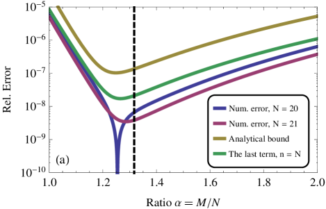
(a)

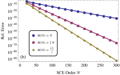
(b)

Figure 1: Performance of the SCE versus the parameter $\alpha$ and order $N$. (a) Relative error of the SCE as a function of $\alpha=M\left(N\right)/N$. $g$ is fixed at $1$. Shown are measured errors for $N=20$ and $21$. Also plotted is the analytical bound from (LABEL:Total_Error_Bound), and the last, $n=N$ term in (LABEL:SCE_partition) (after summation over $l$, for $N=20$). The analytical bound is quite loose, while the $n=N$ term is a much better estimator of the error of the approximation, especially for $\alpha<\alpha^{*}$ — this property is explored in Direct_1F1_estimation. All the graphs exhibit an optimum choice in the vicinity of $\alpha=1.3$, close to our estimated $\alpha^{*}\approx 1.317$ [(LABEL:alpha_star_value)], marked by the vertical dashed line; note that this value was calculated in the limit of $N\gg 1$. The different behavior of $N=20$ and $N=21$ at optimum is explained in the text. (b) Convergence of the SCE at high order. Plotted are the relative errors of the SCE expansion of the partition function $\mathcal{Z}^{(N)}$ versus the order $N$ (markers). These are plotted for $M=\alpha N$ with $\alpha=1$, $2$, and $\frac{4}{3}$, in order of merit (blue, purple, and yellow, respectively). The coupling $g$ is fixed at $1$. The vertical axis reflects the number of significant digits successfully reproduced by the expansion. The data was fitted with a trend of the form $10^{-AN-B\sqrt{N}+C}$, corresponding to our analytical bound (continuous lines). The fits achieve a $\chi^{2}$ value of $\sim 10^{-2}$ ($\chi^{2}$ is defined in the text). Though even orders admit better accuracy, we evaluate at odd orders to mitigate the sensitivity of the fitted parameters to the exact choice of $\alpha$ near its optimum (cf. the left panel). The fitted values for the coefficient $A$ are $0.072$, $0.200$, and $0.283$, for $\alpha=1$ , $2$, and $\frac{4}{3}$, respectively, representing the minimal amount of decimal places obtained per increment of $N$. The lower bounds for $A\left(\alpha\right)$ as predicted by (LABEL:A_coefficient_bound) are $0.018$, $0.176$ and $0.243$, in agreement with the numerical results. The minimal error shown is roughly $1.5\times 10^{-92}$. Note that in order to obtain this many accurate digits, the intermediate calculations had to be performed with over $300$ digit precision.

1(a)thesubfigure depicts the convergence properties of the SCE as a function of $\alpha$. It shows the error of the expansion for two orders, $N=20$ and $21$, as well as the bound on the error given by (LABEL:Total_Error_Bound), for a moderate coupling strength $g=1$. Lastly, the final $n=N$ term of the expansion is plotted for $N=20$. The analytical bound captures the qualitative behavior of the error, but the last term provides an estimate for the error which is much tighter. This is explored further in Direct_1F1_estimation.

All four error measures exhibit an optimum in the vicinity of $\alpha\approx 1.3$, close to the analytic value we deduced for $\alpha^{*}$. We argued that this point occurs when the dominant domain in the error shifts from $\mathcal{D}_{1}$ to $\mathcal{D}_{2}$. Recall that $R_{1}^{\left(N\right)}$ is always negative, while $R_{2}^{\left(N\right)}$ alternates in sign as $\left(-1\right)^{N}$. If these are continuous functions of $\alpha$, then at $\alpha^{*}$ they should have equal magnitudes. This would imply that for $N$ which is even, at the optimum point they cancel each other to achieve zero error. Indeed, in 1(a)thesubfigure, the expansion with $N=21$ is somewhat better than $N=20$ far from $\alpha^{*}$ (due to the exponential convergence in $N$), but close to $\alpha^{*}$, $N=20$ affords a better approximation. In fact, we note that the location of $\alpha^{*}$ represents the solution of the PMS condition, since (our bound for) the remainder is stationary there for odd $N$; however, whereas the SCE works equally well for even or odd $N$, the PMS breaks down for even $N$ Buckley et al. (1993), despite the fact that the remainder could be canceled completely at even orders.

Next, in 1(b)thesubfigure we push the SCE to large order, evaluating it up to $N=301$. This is performed for $g=1$ and with $\alpha=1$ (as in Ref. Schwartz and Katzav (2008)), $2$ and $\frac{4}{3}$, as an approximation to our estimate for $\alpha^{*}$ and the location of the optima visible in 1(a)thesubfigure. The resulting relative errors are fitted with a curve of the form $10^{C-AN-B\sqrt{N}}$, according to (LABEL:Total_error_functional_form). These fits all achieve a value of $\chi^{2}\sim 10^{-2}$, defined as $\chi^{2}=\left[\frac{1}{L}\sum_{N}\left(C-AN-B\sqrt{N}-\log_{10}\left|R^{\left(N\right)}\big{/}\mathcal{Z}\right|\right)^{2}\right]^{\frac{1}{2}}$, where $R^{\left(N\right)}/\mathcal{Z}$ is the relative error, the sum is over all the data points, and $L$ is their number. Discarding the stretched exponent by setting $B=0$, $\chi^{2}$ jumps to about $\sim 0.2$. The fitted values for the parameter $A$ are $0.072$, $0.200$ and $0.283$, for $\alpha=1$ , $2$, and $\frac{4}{3}$, respectively. These are in agreement with the bounding values $0.018$, $0.176$, and $0.243$, given by (LABEL:A_coefficient_bound).

We continue with a comparison of the SCE with other asymptotic and numerical approximation schemes. These include the methods of super and hyperasymptotics Boyd (1999); Berry and Howls (1990, 1991), Borel remainder summation Negele and Orland (1998); Costin (2008), Padé approximants Bender and Orszag (1978), and the Chebyshev $\tau$ method due to Lanczos Boyd (2001). For an outline of these methods, refer to Competing_Methods.

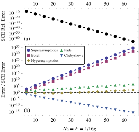
Figure 2: A comparison of the SCE with other asymptotic and numeric schemes, in order of merit (see Competing_Methods): Superasymptotics (i.e. truncation of PT at the least term) Boyd (1999); Borel resummation of the superasymptotic remainder (Negele and Orland, 1998, Sec. 7.2); Padé approximants of PT Bender and Orszag (1978); $3^{\text{rd}}$ level hyperasymptotics Berry and Howls (1990, 1991); SCE (with $\alpha=4/3$); and Lanczos’s Chebyshev $\tau$ approximations of $\mathcal{Z}\left(g\right)$ Boyd (2001). Since the Padé, SCE and Lanczos methods converge and thus can be evaluated to arbitrary order, we choose to compare them with the asymptotic methods at the same order $N=N_{0}=\frac{1}{16g}$ as that used in the superasymptotic expansion. (a) The relative error of the SCE. The horizontal axis is the singulant $F=\frac{1}{16g}$ (cf. Subsection B.B.2thesubsection), and at each point the SCE is evaluated to order $N_{0}=F$, which is the same truncation as the superasymptotic scheme. The line segments are a guide to the eye. (b) The errors produced by the other methods, relative to that produced by the SCE (i.e., the data was normalized by that shown in the top panel). The line segments are a guide to the eye. When evaluated at the same order, the SCE outperforms superasymptotics, Borel tail resummation, and the Padé approximants. Note the extremely similar errors produced by the SCE and hyperasymptotics, which is formally of order $2N_{0}$; this is discussed in the text. Lastly, the Chebyshev $\tau$ method appears more accurate than the SCE, but only because of the specific truncation at $1/16g$. In the large-$N$ limit, the SCE is more rapidly convergent, as demonstrated in 3(b)thesubfigure. The dominance of the SCE in the strongly-coupled regime is not manifest in this comparison, since for $g\gg 1$ the superasymptotic truncation occurs at $N_{0}=0$; however, for fixed and finite $N$, the SCE is vastly superior in this scenario, as depicted in 3(a)thesubfigure.

A comparative plot of all techniques is shown in 2 for different values of weak $g$. By definition, superasymptotics are evaluated up to the least term of PT, which occurs at $N_{0}=\frac{1}{16g}$ (round down). Hyperasymptotics are evaluated up to level 3 (or less, if the procedure halts before). To make a “fair” comparison, the SCE, Padé, and $\tau$ methods are evaluated at $N=N_{0}$, though in principle they converge as $N\rightarrow\infty$.

A striking result of 2 is the similarity of the errors produced by SCE (at order $N_{0}=\frac{1}{16g}$) and hyperasymptotics. This can be explained by the error estimates of both: Revisiting (LABEL:SCE_Stretched_Exponent), we can bound

$$\left(1-\frac{1}{G\left(N_{0}\right)}\right)^{N_{0}} =\left(1-\frac{1}{\frac{1}{2}+\frac{1}{2}\sqrt{1+16g\left(\frac{\alpha}{16g}+2\right)}}\right)^{N_{0}}\approx\left(1-\frac{1}{\frac{1}{2}+\frac{1}{2}\sqrt{1+\alpha}}\right)^{N_{0}}\approx e^{-1.57N_{0}}\,,$$ (48)

where we have substituted $\alpha=\frac{4}{3}$. Notably, at this truncation, we do not yet witness the stretched-exponential behavior which occurs at large $N$, but rather a regular exponent. Adding the factor $\left(\frac{\alpha}{\alpha+1}\right)^{N_{0}}=e^{-0.56N_{0}}$ [(LABEL:Total_error_functional_form) and (LABEL:A_coefficient_bound)], we find that the SCE at order $\frac{1}{16g}$ has an error bound that scales as $\sim e^{-2.12N_{0}}$. Substituting the numerically fitted uniform factor $10^{-0.283N}=e^{-0.65N}$ [cf. 1(b)thesubfigure], an even smaller error of $\sim e^{-2.22N_{0}}$ is obtained. In comparison, examining the exponential factors in (LABEL:Anharmonic_Z4_Hypersymptotic_Error), we see a scaling of $\exp\left\{-\left(1+\sum_{s=1}^{S}\frac{\ln 2}{2^{s-1}}\right)N_{0}\right\}$ with $S=-\log_{2}\left(16g\right)$. For $2$ and $3$ stages, the scaling so obtained is $e^{-2.04N_{0}}$ and $e^{-2.21N_{0}}$, respectively, very close to the scaling for infinitesimal $g$ (when $S$ is very large), $e^{-\left(1+2\ln 2\right)N_{0}}\approx e^{-2.386N_{0}}$ Berry and Howls (1990, 1991). This implies that the SCE to order $N_{0}$ produces an error comparable with the hyperasymptotic trans-series at levels $2$ and $3$. However, the SCE requires only $N_{0}$ terms to achieve this, compared to $\sim\frac{3}{2}N_{0}$ or $\sim\frac{7}{4}N_{0}$ terms required by hyperasymptotics at these stages. If compared with hyperasymptotics when carried through to its conclusion, halting at roughly $2N_{0}$ terms with an error of order $e^{-2.386N_{0}}$, then at order $2N_{0}$ the SCE would result in an error of order $\left(1-\frac{1}{\frac{1}{2}+\frac{1}{2}\sqrt{1+2\times\alpha}}\right)^{2N_{0}}\left(\frac{\alpha}{\alpha+1}\right)^{2N_{0}}\approx e^{-3.44N_{0}}$, which is about $44\%$ faster in terms of its dependence on $N_{0}$.

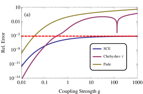
(a)

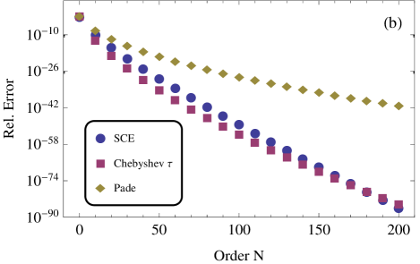
(b)

Figure 3: Comparison of the SCE against numerical methods. (a) The relative error produced by SCE, Padé approximants Bender and Orszag (1978) and the Chebyshev $\tau$ method Boyd (2001) versus $g$ (see Competing_Methods). All methods are evaluated at $N=13$; the SCE is evaluated with $\alpha=\frac{4}{3}$. The SCE outperforms the Padé approximants across a wide range of values for $g$, and outperforms the $\tau$ method for $g\gtrsim 0.1$. This holds for other values of $N$ as well. As $g$ grows larger, the relative errors of the Padé and $\tau$ approximations diverge, though the approximations themselves are finite. The dashed red line shows the ultimate error of the SCE for $g\rightarrow\infty$, about $7.83\times 10^{-6}$. This value was calculated by comparing the coefficients of $g^{-\frac{1}{4}}$ in the large-$g$ expansions of (LABEL:Z_analytic) [which is $\frac{1}{2}\Gamma\left(\frac{1}{4}\right)$] and (LABEL:SCE_partition) [obtained by taking $1-1/G\to 1$ and $\sqrt{\frac{2}{G}}\to\left(gK\right)^{-\frac{1}{4}}$]. The sharp dip in the error of the $\tau$ method near $g\approx 150$ is due to the the error switching signs across that value, so at the crossover the relative error vanishes. This does not occur with the SCE since we evaluate at an odd order $N$ [cf. 1(a)thesubfigure]. (b) The relative error produced by the same methods versus the approximation order $N$, up to order $200$. All methods are evaluated at $g=0.01$; the SCE is evaluated with $\alpha=\frac{4}{3}$. The SCE is consistently more accurate than the Padé approximants, and it supersedes the $\tau$ method at roughly $N=180$, which depends on the value of $g$.

We also wish to compare the SCE with convergent methods of approximation. For this comparison, we can again decouple $g$ and the truncation order $N$. From 2 one may deduce that the SCE is numerically comparable to the Padé approximants, and inferior to the Chebyshev $\tau$ method, but that is misleading. First, the immediate advantage of the SCE over the other methods is its uniform convergence in $g$ for all positive values, and in particular for $g\gtrsim 1$, a domain which was not represented in 2, since there the superasymptotic series is trivial (truncated at the zeroth term) for $g>\frac{1}{16}$. Both the Padé approximants and the $\tau$ approximations are rational functions of $g$, where the numerator and denominator are of identical order in $g$; as such, for a fixed order $N$, they will tend to a constant as $g\rightarrow\infty$. $\mathcal{Z}\left(g\right)$ decays to zero for $g\rightarrow\infty$ (the anharmonicity compresses the oscillator’s spatial distribution), so the relative error of these schemes will diverge for larger $g$. The SCE’s supremacy over these techniques for larger couplings is demonstrated in 3(a)thesubfigure.

Second, we contend that even for $g\ll 1$, while the SCE is initially less accurate, it overtakes other methods at high enough orders. We show this numerically in 3(b)thesubfigure for $g=\frac{1}{100}$. The SCE converges markedly faster than the Padé approximants for any $N$, while for smaller $N$ it is outperformed by the $\tau$ method. However, at sufficiently large order — $N\approx 180$, in this case — the SCE overtakes it. This crossover point depends on $g$; for example, for $g=\frac{2}{100}$, it occurs as early as $N=90$. It is also worth mentioning that at a given order, evaluating the SCE is much quicker than any of the other methods.

V Non-Perturbative SCE: The Double-Well Potential

Now that the convergent nature of the SCE has been observed, we can examine a more intricate case, that of the double-well potential, corresponding to a negative quadratic part of the potential ($\gamma<0$ in (LABEL:anharmonic_potential_V)). This has the effect of flipping the sign of the quadratic term in (LABEL:Z_definition). It is an interesting test case, since the quadratic Hamiltonian alone is not stable, and thus the PT expansion must be performed about the minima of the potential, instead of around $g=0$ and the $x$ origin. However, we will show that the SCE captures the correct partition function even when expanding around a harmonic zeroth order approximation.

The partition function is now given by

$$\mathcal{Z}\left(g\right)=\frac{\pi}{\sqrt{16g}}e^{\frac{1}{32g}}\left[I_{\frac{1}{4}}\left(\frac{1}{32g}\right)+I_{-\frac{1}{4}}\left(\frac{1}{32g}\right)\right]\,,$$ (49)

with $I_{\nu}\left(x\right)$ the modified Bessel functions of the first kind Abramowitz and Stegun (1964). Carrying through the same analysis as in II, we find that now the self-consistent harmonic coefficient $G$ becomes

$$G_{DW}\left(M\right)=-\frac{1}{2}+\frac{1}{2}\sqrt{1+16g\left(M+2\right)}>0\,,$$ (50)

where we have chosen the positive root for $G$, so that the integrals of $\exp\left(-\frac{1}{2}Gx^{2}\right)$ are convergent. We then find that the SCE for the double-well partition function is the same power series as (19), apart from the replacement $\left(1-1/G\right)\to\left(1+1/G\right)>1$.

In III we established that the exponential convergence of the SCE was due to the large-$N$ scaling of its coefficients. For the double-well potential, these coefficients are unchanged and exponential convergence is preserved. However, the factor $\left(1-1/G\right)^{N}$, which previously contributed a decaying stretched exponent, now becomes a divergent $\left(1+1/G\right)^{N}$ factor. Furthermore, note that the small-$Mg$ limit of (LABEL:Double_Well_G) gives $G_{DW}=0$ and not $1$, so that at low orders, $G^{-1}\approx\left(4gM\right)^{-1}$ is very large. However, at large order, this factor behaves again as a stretched exponent, which will eventually be overwhelmed by the exponential convergence for sufficiently large $N$, once [cf. (LABEL:SCE_Stretched_Exponent) and (LABEL:A_coefficient_bound)]

$$N\geq N_{c}\left(\alpha,g\right)=-\sqrt{\frac{1}{16g\alpha}}\Bigg{/}\ln\left(\frac{\alpha}{\alpha+1}\right)\,.$$ (51)

For our optimal $\alpha^{*}\approx\frac{4}{3}$, this is satisfied already at order $N=1$ for $g\gtrsim 0.2$. This convergence is demonstrated in 4(a)thesubfigure. The positivity of the stretched exponent implies that for the double-well system, convergences is not uniform for all $g>0$, but only for $g\geq\epsilon>0$, i.e. on any interval of finite $g$. This is of course unavoidable, since at $g=0$ the potential is not bound from below and the partition function cannot be defined.

We attribute the initial divergence of the SCE at low orders to an incompatibility between two conflicting goals. The first is that the SCE zeroth order potential $V_{0}\left(x\right)=\frac{1}{2}Gx^{2}$ preserve the moments $\left\langle x^{2M}\right\rangle$; the second goal is that it should revert to the original system when $g\rightarrow 0$, i.e. reduce to $V\left(x\right)=-\frac{1}{2}x^{2}$. Of course, the latter potential has ill-defined moments, as the original system relies on the quartic term for stability. Faced with this conflict, our formulation of the SCE favors the first goal. Let us also note that the solution in (LABEL:Double_Well_G) is but one of two for $G$, borne of a quadratic equation, with the other being $G=-\frac{1}{2}-\frac{1}{2}\sqrt{1+16g\left(M+2\right)}$, which does revert to the correct potential when $g=0$; however, this $G$ is strictly negative, contrary to the requirement that integrals of $\exp\left(-\frac{1}{2}Gx^{2}\right)$ converge.

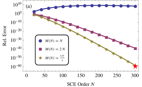
(a)

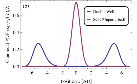
(b)

Figure 4: The convergence of the SCE for the case of a double-well potential. We examine the barely binding case of $g=0.01$, so that the differences between this case and the previous Sections are accentuated. (a) The double-well counterpart of 1(b)thesubfigure: Shown is the numerical accuracy of the SCE, evaluated for $\alpha=1$, $2$, and $\frac{4}{3}$ (markers). Note that all three trends converge, though for the $\alpha=1$ case, the exponential convergence has barely begun to rein in the divergent stretched exponent at $N\approx 200$, showing that a proper choice of $\alpha$ is critical to the effectiveness of the approximation. All points are evaluated at odd order [cf. 1(a)thesubfigure]. Against the data we fit a trend line of the form $10^{C-AN+B\sqrt{N}}$ (solid lines), and the fitted values of $A$ are $0.075,$ $0.197$, and $0.282$ for $\alpha=1$, $2$, and $\frac{4}{3}$, respectively, essentially the same as those fitted in 1(b)thesubfigure. (b) The Boltzmannian (normalized) distributions $e^{-\beta V\left(x\right)}/\mathcal{Z}$ of the double-well potential $V\left(x\right)=-\frac{1}{2}x^{2}+gx^{4}$, and the zeroth-order approximation $V\left(x\right)=+\frac{1}{2}Gx^{2}$ around which the SCE is expanded. This plot corresponds to the point marked by a red star in the left panel, where $N=301$ and $\alpha=\frac{4}{3}$. Note how the SCE’s reference system bears little resemblance to the approximated one.

Lastly, we examine the behavior of the SCE if the quadratic coefficient $\gamma$ is varied continuously. Let us begin with a positive $\gamma$, and steadily decrease it. The effective coupling $g=\frac{g_{0}}{\beta\gamma^{2}}$ starts to increase, while the solution for $G$ is on the branch given by (LABEL:First_order_G). As $\gamma\rightarrow 0^{+}$, $g\rightarrow\infty$ and so does $G$. As $\gamma$ crosses zero, $G\rightarrow\infty$ for $\gamma\rightarrow 0^{-}$, but as $\left|\gamma\right|$ increases, $G$ descends from infinity along the double-well branch in (LABEL:Double_Well_G).

Strikingly, we have shown that the SCE provides a means to write down a perturbative expansion to a non-perturbative system (in the sense that the quartic contribution is essential to the stability of the harmonic term). Furthermore, this is despite the fact that the reference harmonic model around which the SCE is performed is very different from the original system, as illustrated in 4(b)thesubfigure. However, the SCE manages to coerce the calculation into the correct result. For the ODM/OPT/LDE this was previously stated in Ref. Buckley et al. (1993) and shown in Ref. Guida et al. (1996), though they derive looser functional forms for the convergence rate (i.e., stretched instead of normal exponential convergence).

Naturally, a proper perturbative treatment of the problem would be to expand around the two minima of the double-well, with the associated degenerate ground states and tunneling between them. Of course, a standard PT around the minima would still be formally divergent and would require incorporating instantons (tunneling events) Zinn-Justin (2002). However, our goal here was to demonstrate the power of the SCE, and in particular its flexibility in formulating an exact approximation scheme; note that the SCE is convergent to the correct result, even when expanding around the local maximum ($x=0$) and without the inclusion of non-perturbative contributions, such as instantons. What is more, the discrete mapping between the anharmonic and double-well potentials is instructive to analyze and gain intuition about, before we generalize it to a continuous transition in the complex plane in VII.

VI General Power-Law Perturbations

A SCE may be performed in the case of a general perturbation $g\left|x\right|^{q}$. We assume that $q>2$, and that $g$ may be complex but has a positive real part. Expanding again around a modified $\frac{1}{2}Gx^{2}$ harmonic oscillator, the partition function is now

$$\mathcal{Z}^{\left(N\right)}=\sqrt{\frac{2}{G}}\sum_{n=0}^{N}\left(1-\frac{1}{G}\right)^{n}\sum_{l}^{n}\frac{1}{n!}\binom{n}{l}\Gamma\left(\frac{1}{2}+n+\left(\frac{q}{2}-1\right)l\right)\left[\frac{\left(1-G\right)G^{\frac{q-2}{2}}}{2^{\frac{q}{2}}g}\right]^{-l}\,.$$ (52)

One can then show that the self-consistency condition for the moment $\left\langle x^{2M}\right\rangle$ is

$$\left(\frac{G}{2}\right)^{\frac{q}{2}}-\frac{1}{2}\left(\frac{G}{2}\right)^{\frac{q}{2}-1}-\frac{g}{M}C_{q}\left(M\right)=0\,,\qquad C_{q}\left(M\right)=\frac{\Gamma\left(M+\frac{q}{2}+\frac{1}{2}\right)}{\Gamma\left(M+\frac{1}{2}\right)}-\frac{\Gamma\left(\frac{q}{2}+\frac{1}{2}\right)}{\Gamma\left(\frac{1}{2}\right)}\,,$$ (53)

which has at least one solution for $G>1$. Let us first examine the limiting behaviors of the solution, which we will use below. Asymptotically, for large $M$ and fixed $g$ and $q$, $C_{q}\left(M\right)\sim M^{\frac{q}{2}}$ and thus

$$G=2g^{\frac{2}{q}}M^{1-\frac{2}{q}}+\frac{2}{q}+\mathcal{O}\left(1/g^{\frac{2}{q}}M^{1-\frac{2}{q}}\right)\,.$$ (54)

For small $\frac{g}{M}C_{q}$, $G$ is close to unity, or approximately

$$G\approx 1-\frac{1}{q-2}+\sqrt{\left(\frac{1}{q-2}\right)^{2}+2^{1+\frac{q}{2}}\frac{gC_{q}\left(M\right)}{M\left(q-2\right)}}\,,$$ (55)

which is exact for $q=4$. If $G-1$ is small but $M\gg q$ (i.e., $gM^{\frac{q}{2}-1}$ is small but $M$ is large), then a simpler limit applies,

$$G\approx 1+2^{\frac{q}{2}}gM^{\frac{q}{2}-1}\,.$$ (56)

Going back to the expansion for $\mathcal{Z}$, it now becomes

$$\mathcal{Z}^{\left(N\right)}=\sqrt{\frac{2}{G}}\sum_{n=0}^{N}\left(1-\frac{1}{G}\right)^{n}\sum_{l=0}^{n}\binom{n}{l}\frac{\left(-1\right)^{l}}{n!}\left(\frac{C_{q}\left(M\right)}{M}\right)^{-l}\Gamma\left(\frac{1}{2}+n+\left(\frac{q}{2}-1\right)l\right)\,.$$ (57)

To first prove the possibility of non-divergence, we can generalize case 3 of Proposition 1. The dominant term in the $l$ summation will occur at the index $l=0$ if

$$1 \geq\frac{M}{C_{q}}\frac{n-l}{l+1}\frac{\Gamma\left(n+\frac{q-2}{2}\left(l+1\right)+\frac{1}{2}\right)}{\Gamma\left(n+\frac{q-2}{2}l+\frac{1}{2}\right)}\Biggr{|}_{l=0}=\frac{M}{C_{q}}n\frac{\Gamma\left(n+\frac{q-2}{2}+\frac{1}{2}\right)}{\Gamma\left(n+\frac{1}{2}\right)}\,.$$ (58)

The rhs scales as $n^{q/2}M^{1-q/2}$, hence the critical $M$ scales as $M\sim N^{\frac{q}{q-2}}$. Now, the partition function is once more bounded by the sum of the $l=0$ terms, which again produces the bound

$$\mathcal{Z}^{\left(N\right)}\apprle\sqrt{\frac{N}{G}}\sim N^{\frac{1}{2}\left(1-p\left(1-\frac{2}{q}\right)\right)}\rightarrow 0\,,$$ (59)

if $M\sim N^{p}$ and $p>\frac{q}{q-2}$, in agreement with the critical value we had just obtained.

Let us now proceed to generalize cases 2a and 2b. The error can once again be calculated by

$$\lim_{N\rightarrow\infty}\mathcal{Z}^{\left(N\right)} =\lim_{N\rightarrow\infty}\int_{-\infty}^{\infty}e^{-\frac{1}{2}Gx^{2}}\sum_{n=0}^{N}\frac{1}{n!}\left(-\left[\frac{1}{2}\left(1-G\right)x^{2}+gx^{q}\right]\right)^{n}dx$$

$$=\lim_{N\rightarrow\infty}\sqrt{\frac{2}{G}}\int_{0}^{\infty}e^{-u}\sum_{n=0}^{N}\frac{1}{n!}\left(1-\frac{1}{G}\right)^{n}\left(u-\frac{Gg}{\left(G-1\right)}\left(\frac{2}{G}\right)^{\frac{q}{2}}u^{\frac{q}{2}}\right)^{n}\frac{du}{\sqrt{u}}$$

$$=\lim_{N\rightarrow\infty}\sqrt{\frac{2K}{G}}\sum_{n=0}^{N}\left(1-\frac{1}{G}\right)^{n}\frac{K^{n}}{n!}\int_{0}^{\infty}e^{-Kv}v^{n}\left(1-v^{r}\right)^{n}\frac{dv}{\sqrt{v}}\,,$$ (60)

with $K=\left(\frac{C_{q}\left(M\right)}{M}\right)^{1/r}$ and $r=\frac{q-2}{2}$. For $q=4$, we have $r=1$ and $C_{4}\left(M\right)=M^{2}+2M$, and thus $K=M+2$, which is consistent with its definition in the previous Sections. Apart from the power of $v$ in the third factor of the integrand, this equation is the same as that for $q=4$ [see (LABEL:Z_limit_integral_form)]. In particular, the domains defined in (LABEL:Definition_of_D_Domains) still apply for the analysis of the error of this expansion. Our aim is again to show that this expansion can be constructed to converge exponentially with a suitable choice of $M\left(N\right)=\alpha N$. Note that for any fixed value of $q$, in the limit of very large $M\gg q$, $K=M+\frac{q^{2}}{4\left(q-2\right)}+o\left(1\right)$, so up to constants they are asymptotically equivalent at large order. Realizing this, we choose not to reformulate the convergence criteria in terms of $K$ (i.e., we do not redefine $\alpha=K/N$), since the moment $M$ carries a physical interpretation, while its mapping to $K$ is not universal, as it clearly depends on the detailed structure of the theory.

VI.1 The Domain $\mathcal{D}_{1}$

In this domain, we again bound the sum of truncated terms with the aid of the Monotone Convergence Theorem,

$$-R_{1,q}^{\left(N\right)} =\sqrt{\frac{2K}{G}}\sum_{n=N^{\prime}}^{\infty}\frac{K^{n}}{n!}\left(1-\frac{1}{G}\right)^{n}\int_{0}^{1}e^{-Kv}v^{n}\left(1-v^{r}\right)^{n}\frac{dv}{\sqrt{v}}<\sqrt{\frac{2K}{G}}\sum_{n=N^{\prime}}^{\infty}\frac{K^{n}}{n!}\left(1-\frac{1}{G}\right)^{n}\int_{0}^{1}e^{-Kv-nv^{r}}v^{n-\frac{1}{2}}dv\,.$$ (61)

Our goal now is to bound the power $v^{r}$ in the exponent from below by a linear approximation. If $q<4$ then $r<1$, and $v^{r}$ is a concave function which on the interval $\left[0,1\right]$ is simply bounded by $v$. This will reproduce the eventual $\left(\frac{K}{K+N^{\prime}}\right)^{N}$ result obtained for $q=4$. Let us then focus on $q>4$, so henceforth $r>1$: As $v^{r}$ is now a convex function, it is bounded by any line drawn tangential to it. Denoting by $v_{0}>0$ the arbitrary point where we draw this tangent, we can bound

$$v^{r} >rv_{0}^{r-1}\left(v-v_{0}\right)+v_{0}^{r}=rv_{0}^{r-1}v-\left(r-1\right)v_{0}^{r}\,.$$ (62)

Plugging this in, the error is bounded by

$$-R_{1,q}^{\left(N\right)} <\sqrt{\frac{2K}{G}}\sum_{n=N^{\prime}}^{\infty}\frac{K^{n}}{n!}\left(1-\frac{1}{G}\right)^{n}e^{n\left(r-1\right)v_{0}^{r}}\int_{0}^{\infty}e^{-\left(K+nrv_{0}^{r-1}\right)v}v^{n-\frac{1}{2}}dv$$

$$=\sqrt{\frac{2K}{G}}\sum_{n=N^{\prime}}^{\infty}\frac{K^{n}}{n!}\left(1-\frac{1}{G}\right)^{n}e^{n\left(r-1\right)v_{0}^{r}}\frac{\Gamma\left(n+\frac{1}{2}\right)}{\left(K+nrv_{0}^{r-1}\right)^{n+\frac{1}{2}}}$$

$$<\sqrt{\frac{2K}{GN^{\prime}\left(K+N^{\prime}rv_{0}^{r-1}\right)}}\left(1-\frac{1}{G}\right)^{N^{\prime}}\sum_{n=N^{\prime}}^{\infty}\left(\frac{Ke^{\left(r-1\right)v_{0}^{r}}}{K+N^{\prime}rv_{0}^{r-1}}\right)^{n}\,,$$ (63)

This is a geometric series which converges only if its quotient is smaller than one, namely if

$$K\left(e^{\left(r-1\right)v_{0}^{r}}-1\right)-N^{\prime}rv_{0}^{r-1}<0\,.$$ (64)

This condition is satisfied trivially for $r=1$ (i.e. $q=4$), where we saw that $\mathcal{D}_{1}$ is necessarily convergent. For $r>1$, we note that for $v_{0}=0$ the left-hand side of (LABEL:tangent_convergence_criteria) equals $0$. However, since $e^{\left(r-1\right)v_{0}^{r}}$ can be expanded in powers of $v_{0}^{r}$, the first non-vanishing derivative of the lhs is the $\left(r-1\right)$-th, giving $N^{\prime}\left(-r!\right)<0$. Thus, this equation is satisfied at least in the neighborhood of $0^{+}$. Indeed, for $v_{0}\ll 1$, we can expand

$$K\left(r-1\right)v_{0}^{r}-N^{\prime}rv_{0}^{r-1}<0\,,$$ (65)

giving us a self-consistent solution as long as $v_{0}<\frac{r}{\left(r-1\right)}\frac{N^{\prime}}{K}$.

Next, we wish to optimize the bound. Clearly, the quotient diverges at large $v_{0}$ due to the exponent $e^{\left(r-1\right)v_{0}^{r}}$, so the interval over which it is smaller than unity is finite, and thus contains a minimum. Differentiating with respect to $v_{0}$ and setting to zero, we find

$$\frac{K}{N^{\prime}}+rv_{0}^{r-1}=v_{0}^{-1}\,.$$ (66)

For $v_{0}\rightarrow 0$ the rhs diverges, while for large $v_{0}$ the lhs is dominant. Since at $v_{0}=\frac{N^{\prime}}{K}$ the lhs reads $\frac{K}{N^{\prime}}+r\left(\frac{K}{N^{\prime}}\right)^{1-r}$ and the rhs is $\frac{K}{N^{\prime}}$, this implies that the root of (LABEL:optimal_tangent) satisfies $v_{0}<\frac{N^{\prime}}{K}$. For $r=2$, it is solved explicitly by

$$v_{0}=\frac{1}{4}\left(\sqrt{\left(\frac{K}{N^{\prime}}\right)^{2}+8}-\frac{K}{N^{\prime}}\right)\sim\frac{N^{\prime}}{K}-2\left(\frac{N^{\prime}}{K}\right)^{3}\,.$$ (67)

From now we set $v_{0}$ to be the root of (LABEL:optimal_tangent). Inserting it into the error bound, we have

$$-R_{1,q}^{\left(N\right)} <\sqrt{\frac{2K}{GN^{\prime}\left(K+N^{\prime}rv_{0}^{r-1}\right)}}\left(1-\frac{1}{G}\right)^{N^{\prime}}\sum_{n=N^{\prime}}^{\infty}Q_{1}^{n}=\sqrt{\frac{2Kv_{0}}{G\left(N^{\prime}\right)^{2}}}\left(1-\frac{1}{G}\right)^{N^{\prime}}\frac{Q_{1}^{N^{\prime}}}{1-Q_{1}}\,,$$ (68)

$$Q_{1}=\frac{Kv_{0}}{N^{\prime}}e^{\frac{r-1}{r}\left(1-\frac{K}{N^{\prime}}v_{0}\right)}<1\,.$$ (69)

VI.2 The Domain $\mathcal{D}_{2}$

In this domain, the error is bounded by the Lagrange remainder,

$$\left|R_{2,q}^{\left(N\right)}\right| <\sqrt{\frac{2K}{G}}\frac{K^{N^{\prime}}}{N^{\prime}!}\left(1-\frac{1}{G}\right)^{N^{\prime}}\int_{1}^{\infty}e^{-Kv}v^{N^{\prime}}\left(v^{r}-1\right)^{N^{\prime}}\frac{dv}{\sqrt{v}}\,.$$ (70)

For $q>4$ we can perform a bound which was too loose for $q=4$ but is tight for larger powers. We may write

$$\left|R_{2,q}^{\left(N\right)}\right| =\sqrt{\frac{2K}{G}}\frac{K^{N^{\prime}}}{N^{\prime}!}\left(1-\frac{1}{G}\right)^{N^{\prime}}\int_{1}^{\infty}e^{-Kv}v^{N^{\prime}}\left(v^{r}-1\right)^{N^{\prime}}\frac{dv}{\sqrt{v}}$$

$$<\sqrt{\frac{2K}{G}}\frac{K^{N^{\prime}}}{N^{\prime}!}\left(1-\frac{1}{G}\right)^{N^{\prime}}\int_{1}^{\infty}e^{-Kv}v^{\left(r+1\right)N^{\prime}}\frac{dv}{\sqrt{v}}$$

$$<\sqrt{\frac{2K}{G}}\frac{K^{N^{\prime}}}{N^{\prime}!}\left(1-\frac{1}{G}\right)^{N^{\prime}}\frac{\Gamma\left(\left(r+1\right)N^{\prime}+\frac{1}{2}\right)}{K^{\left(r+1\right)N^{\prime}+1/2}}$$

$$<\sqrt{\frac{2}{G}}\left(1-\frac{1}{G}\right)^{N^{\prime}}\frac{\left(\left(r+1\right)N^{\prime}\right)!}{K^{rN^{\prime}}N^{\prime}!}\,.$$ (71)

For $2<q<4$, we can write

$$\left|R_{2,q}^{\left(N\right)}\right| \Bigg{/}\sqrt{\frac{2K}{G}}\frac{K^{N^{\prime}}}{N^{\prime}!}\left(1-\frac{1}{G}\right)^{N^{\prime}}=\int_{1}^{\infty}e^{-Kv}v^{N^{\prime}}\left(v^{r}-1\right)^{N^{\prime}}\frac{dv}{\sqrt{v}}$$

$$=e^{-K}\int_{0}^{\infty}e^{-Kv}\left(v+1\right)^{N^{\prime}-\frac{1}{2}}\left(\left(v+1\right)^{r}-1\right)^{N^{\prime}}dv$$

$$<e^{-K}r^{N^{\prime}}\int_{0}^{\infty}e^{-Kv}\left(v+1\right)^{N^{\prime}-\frac{1}{2}}v^{N^{\prime}}dv$$ (72)

where he have used Bernoulli’s inequality $\left(1+x\right)^{r}\leq 1+rx$ for positive $x$ and $0\leq r\leq 1$. Note that we now have to evaluate the same expression for $R_{2}^{\left(N\right)}$ as we did for $q=4$ in (LABEL:R2_for_q_4), only multiplied by $r^{N^{\prime}}$. Since $q<4$, we have $r=\frac{q-2}{2}<1$, and thus $r^{N^{\prime}}<1$. This means that the requirements imposed on $K\left(N\right)$, and consequently on $M\left(N\right)$, are more relaxed than for $q=4$, and thus the expansion can be made convergent for any $2<q<4$.

VI.3 Rates and Domains of Convergence

Collecting the contributions from all domains and cases, we find the total bound on the error to be

$$R_{q}^{\left(N\right)} <\sqrt{\frac{2}{G}}\left(1-\frac{1}{G}\right)^{N^{\prime}}\begin{cases}\sqrt{\frac{Kv_{0}}{\left(N^{\prime}\right)^{2}}}\frac{Q_{1}^{N^{\prime}}}{1-Q_{1}}+\frac{\left(\left(r+1\right)N^{\prime}\right)!}{K^{rN^{\prime}}N^{\prime}!}\,,&r>1\\ \sqrt{\frac{K^{2}}{\left(N^{\prime}\right)^{3}}}\left(\frac{K}{K+N^{\prime}}\right)^{N^{\prime}-\frac{1}{2}}+\frac{\left(2r\right)^{N^{\prime}}}{\sqrt{2K}}e^{-K}+\frac{2}{K}\frac{\left(2rN^{\prime}\right)}{N^{\prime}!}^{N^{\prime}}\left(\frac{2N^{\prime}}{K}+1\right)^{N^{\prime}+1}e^{-2N^{\prime}-\frac{K}{2}-\frac{K^{2}}{2N^{\prime}+K}}.&r\leq 1\end{cases}$$ (73)

This bound is similar in structure to that in III, and can be shown to converge if $K/N$ is sufficiently large. Let us again start from the case $M=\alpha N$ for constant $\alpha$ (case 2b). Recalling that $K=\left(\frac{C_{q}\left(M\right)}{M}\right)^{1/r}=M+\frac{q^{2}}{8r}+o\left(1\right)>M$, we see that picking such $M$ ensures $K/N>\alpha$. Thus, by replacing $K/N^{\prime}\rightarrow\alpha$, we can find the minimal value of $\alpha$ required for convergence in the selection of the self-consistent moment $\left\langle x^{2M}\right\rangle$.

Specifically, all error components are exponential in $N$, that is, scale as some $Q^{N}$. For $r>1$, from $\mathcal{D}_{1}$ we have $Q_{1}<1$ given by (LABEL:Quotient_D1_general_q), while from $\mathcal{D}_{2}$ we have

$$Q_{2}=\alpha^{-r}\left(\frac{r+1}{e}\right)^{r+1}e\Rightarrow\alpha_{c}=\frac{1}{e}\left(r+1\right)^{1+\frac{1}{r}}\,.$$ (74)

For $r\leq 1$, $Q_{1}=$$\frac{\alpha}{\alpha+1}$ and $\mathcal{D}_{2}$ has two components, which are

$$Q_{2A}=e^{-\alpha}2r\Rightarrow\alpha_{c,A}=\ln\left(2r\right)\,,$$ (75)

$$Q_{2B}=2r\left(\frac{2}{\alpha}+1\right)e^{-1-\frac{\alpha}{2}-\frac{\alpha^{2}}{\alpha+2}}\,,$$ (76)

and $\alpha_{c,B}$ can be found numerically for each $q$. Note that $Q_{2A,B}$ are both scaled by $r<1$ relative to their values for $r=1$ while $Q_{1}$ is unchanged, so all interesting features will occur for values of $\alpha$ smaller then those in III, namely below $\alpha^{*}=1.317$ [see (LABEL:alpha_star_value)]. $Q_{2A}<Q_{2B}$ for all $\alpha<1.42$ (found numerically), thus for all $r<1$, $Q_{2B}$ determines both the critical $\alpha_{c}$ or the optimal $\alpha^{*}$ exclusively (ergo $Q_{2B}$ is the only relevant $Q_{2}$ for $r\leq 1$).

$x^{q}$	$r=\frac{q}{2}-1$	PT Divergence	$\alpha_{c}$		$\alpha^{*}$		$1-Q^{*}$	$-\log_{10}Q^{*}$	$\alpha_{num}^{*}$	$-\log_{10}Q_{num}$
$x^{3}$	$\frac{1}{2}$	$n^{n/2}$	0.	613	0.	981	$5.05\times 10^{-1}$	$3.05\times 10^{-1}$	1.10	$5.38\times 10^{-1}$
$x^{4}$	1	$n^{n}$	0.	976	1.	317	$4.32\times 10^{-1}$	$2.45\times 10^{-1}$	1.33	$2.83\times 10^{-1}$
$x^{6}$	2	$n^{2n}$	1.	91	2.	08	$1.54\times 10^{-1}$	$7.29\times 10^{-2}$	1.80	$9.4\times 10^{-2}$
$x^{8}$	3	$n^{3n}$	2.	34	2.	38	$5.63\times 10^{-2}$	$2.52\times 10^{-2}$	2.25	$2.6\times 10^{-2}$
$x^{10}$	4	$n^{4n}$	2.	750	2.	761	$1.52\times 10^{-2}$	$6.64\times 10^{-3}$	2.70	$7.1\times 10^{-3}$
$x^{12}$	5	$n^{5n}$	3.	1585	3.	1605	$3.05\times 10^{-3}$	$1.33\times 10^{-3}$	3.20	$1.5\times 10^{-3}$
$x^{2r+2}$	$r\gg 1$	$n^{rn}$	$\frac{r+\ln r+1}{e}$				$\frac{1}{er}\left(\frac{e}{r}\right)^{r}$

Table 1: Convergence of the SCE for varying anharmonicity $g|x|^{q}$. The columns are: power of perturbation $x^{q}$; $r=\frac{q}{2}-1$; the large-order divergence of the summand in the standard PT expansion, $a_{n}\propto\Gamma\left(\frac{qn}{2}\right)/n!\sim n^{rn}$; the upper bound on the minimal value of $\alpha$ necessary for convergence, $\alpha_{c}$, as predicted by our analytical error bound; the optimal value for our bound, $\alpha^{*}$; the base of the uniform exponential error at $\alpha^{*}$, $Q^{*}$ (i.e. $R\sim\left(Q^{*}\right)^{N}$), specified by its distance from unity; $\log_{10}Q^{*}$, showing the minimal amount of significant digits obtained per increment of the SCE order $N$; $\alpha_{num}^{*}$, the numerically-obtained approximate true value of the optimum; and $\log_{10}Q_{num}$, the value obtained by numerical evaluation and least-squares fitting, for $\alpha_{num}^{*}$. Note that as $r$ is increased, $\alpha^{*}$ approaches $\alpha_{c}$, and thus the base $Q^{*}$ approaches unity. Since the analytical bound is not very tight for $q\neq 4$, the true optimum value $\alpha_{num}^{*}$ is actually smaller than $\alpha_{c}$. Lastly, the final row shows the large $q\gg 1$ leading order approximations of $\alpha_{c}$ and $Q^{*}$.

In order to asses the applicability of SCE for anharmonicities with $q\neq 4$, we list the values of the critical $\alpha_{c}$ and the optimal $\alpha^{*}$ for the first few integer perturbation powers $q>2$ in 1. $\alpha_{c}$ is given by (LABEL:critical_alpha_D2_large_r_Q2) for $r>1$, or obtained numerically by equating $Q_{2B}$ in (LABEL:Q2B_small_r) to unity for $r<1$. $\alpha^{*}$ is found numerically by equating the appropriate $Q_{2}$ to the corresponding $Q_{1}$, either that obtained by setting $K/N^{\prime}\rightarrow\alpha$ in (LABEL:Quotient_D1_general_q), or $\frac{\alpha}{\alpha+1}$.

For larger orders of anharmonicity, the optimal value $\alpha^{*}$ tends towards $\alpha_{c}$. This is because $\alpha_{c}$ grows large, restricting us to larger values of $\alpha$. However, at large $\alpha$ we find that $Q_{1}\rightarrow 1^{-}$, so the conditions $Q_{2}=Q_{1}$ and $Q_{2}=1$ become virtually identical. We may use this intuition to estimate the convergence rate for very high anharmonicities $r\gg 1$: By substituting $K/N^{\prime}\rightarrow\alpha$ and putting $v_{0}=\frac{1}{\alpha}-\delta v$ in (LABEL:optimal_tangent), we can find the post-leading correction $\delta v$,

$$\alpha\delta v=\frac{r}{r^{2}+\alpha^{r}}\,.$$ (77)

Plugging this into (LABEL:Quotient_D1_general_q),

$$Q=\alpha v_{0}e^{\frac{r-1}{r}\left(1-\alpha v_{0}\right)}=\left(1-\alpha\delta v\right)e^{\frac{r-1}{r}\alpha\delta v}\approx e^{-\frac{\alpha\delta v}{r}}=e^{-\frac{1}{r^{2}+\alpha^{r}}}\,,$$ (78)

and we now assume $\alpha=\alpha_{c}$, given by (LABEL:critical_alpha_D2_large_r_Q2). This gives values in good agreement with the values in 1, especially for $r\geq 4$. For the $q,r\gg 1$ limit, we discard the $r^{2}$ factor. Since $\alpha_{c}\sim r$, we require all corrections up to $\mathcal{O}\left(1\right)$ to find the limit of $\alpha^{r}$. The asymptotic form of (LABEL:critical_alpha_D2_large_r_Q2) is

$$\alpha_{c}=\left(r+\ln r+1\right)/e+\mathcal{O}\left(\left(\ln r\right)^{2}/r\right)\,.$$ (79)

This yields

$$1-Q \sim 1-e^{\frac{1}{\alpha_{c}^{r}}}\sim\left[\frac{\left(r+\ln r+1\right)}{e}\right]^{-r}\approx\frac{1}{re}\left(\frac{r}{e}\right)^{-r}\,.$$ (80)

While in principle the SCE is convergent for all $q$, 1 shows that the exponential convergence rate decreases upon increasing $q$. However, it should be noted that these bounds are not particularly tight as compared with the numerically fitted values (as demonstrated in IV for $q=4$; additional numerical results are listed in the table). Furthermore, they also do not reflect the additional convergent factor of $\left(1-1/G\right)^{N}$, giving a stretched exponential behavior which can assist the convergence rate for weak couplings $g\lesssim 1$. In contrast, we note that for $q>4$, the standard PT series coefficients grow more rapidly than factorially, and thus are not amenable to usual Borel resummation.

Lastly, we note that if $M\left(N\right)\sim N^{p}$ with $1<p<1+\frac{1}{r}$, then $\alpha$ is increasing, and again the error is dominated by domain $\mathcal{D}_{1}$. We may use our $r\gg 1$ estimate for $Q_{1}$, since its derivation only relied on $\alpha\gg 1$, which will be satisfied for sufficiently large $N$ for $p>1$. We then find that

$$Q^{N}\approx e^{-N/\alpha^{r}}=e^{-N\times N^{-r\left(p-1\right)}}=e^{-N^{1-r-rp}}\,,$$ (81)

and convergence is attained if $1<p<1+\frac{1}{r}$. Conversely, the $1-1/G$ factor scales as

$$\left(1-\frac{1}{G}\right)^{N}\sim\left(1-\frac{1}{M^{1-\frac{2}{q}}}\right)^{N}\sim e^{-N\times M^{\frac{2}{q}-1}}\sim e^{-N^{1-p\left(1-2/q\right)}}\,,$$ (82)

which adds an additional $g$-dependent convergent factor for $1<p<\frac{1}{1-2/q}=1+\frac{1}{r}$, that is, for the same range of $p$. This proves case 2a of Proposition 1 for arbitrary $q$.

VII SCE in the Complex Plane: Oscillatory Integrals and Stokes Phenomenon

Following the success of the SCE in treating the anharmonic oscillator, we wish to elucidate other properties of this technique. We would like to explore how the SCE carries over to complex functions, and in particular, oscillatory integrals. Using the results of the previous section for $q=3$, we will treat the Airy function $\mathrm{Ai}\left(z\right)$, which has many applications across the fields of optics, quantum mechanics, fluid mechanics, and elasticity Vallée and Soares (2010).

Our SCE of $\mathrm{Ai}\left(z\right)$ will be performed around the limit $z\rightarrow\infty$, much like its standard asymptotic expansion. We will argue for several different behaviors of the SCE which will depend on where $z$ lies in the complex plane with respect to the Stokes lines Stokes (1864) of the Airy function Vallée and Soares (2010), defined below. This will be reflected in the behavior of the SCE parameter $G$ and a factor $\left(1-\sqrt{z}/\sqrt{G}\right)^{N}$, which is analogous to the stretched exponent of the anharmonic oscillator. We will see three regimes, depending of the argument of $z$: monotonic and uniform exponential convergence, reduced-rate convergence, and initial explosion before eventual convergence.

A previous LDE treatment of a similar problem Blencowe et al. (1998), originally in the context of non-Hermitian Hamiltonians, was restricted to $z=0$, and thus did not observe this rich phenomenology. Furthermore, here will show that the SCE criteria naturally gives rise to a framework which explains these distinct behaviors. Qualitatively, the different regimes in the different Stokes sectors will arise due to two different causes: the first transition, to non-monotonic convergence, is a feature of the solutions for $G$ as a function of $M$ and $z$, and the SCE transitions it smoothly for all $\left|z\right|$. The third behavior is born by a mutual incompatibility between two demands: the self-consistency of an SCE moment $M$, and that at zeroth order $G$ should approach $z$. This discrepancy is a generalization of the double-well behavior of V to the complex plane.

For fixed $\left|z\right|$, all three cases above eventually converge exponentially for large enough $N\sim\left|z\right|^{\frac{3}{2}}$. In particular, the result of the SCE will vary smoothly across the Stokes lines for any argument $z^{\prime}$ within a disk of radius $\left|z\right|$ around the origin.

VII.1 The SCE of $\mathrm{Ai}\left(z\right)$

The Airy function can be put into the integral representation (DLMF, , Eq. (9.5.7))

$$\mathrm{Ai}\left(z\right) =\frac{e^{-\frac{2}{3}z^{3/2}}}{\pi}\int_{0}^{\infty}e^{-z^{1/2}t^{2}}\cos\left(\frac{t^{3}}{3}\right)dt\sim\frac{e^{-\frac{2}{3}z^{3/2}}}{\pi z^{\frac{1}{4}}}\int_{-\infty e^{\frac{1}{4}\arg z}}^{\infty e^{\frac{1}{4}\arg z}}e^{-x^{2}+\frac{i}{3}z^{-\frac{3}{4}}x^{3}}dx$$ (83)

for $\left|\arg\,z\right|<\pi$. A change of integration variables was used to illustrate the correspondence between this case and the previous sections: separating the cosine into its two complex oscillating components, $z^{-\frac{3}{4}}$ can take the role of the nonlinear coupling coefficient $g$ of a cubic perturbation. Crucially, the PT of $\mathrm{Ai\left(z\right)}$ corresponds to its asymptotic expansion for large $z$. We purposefully do not employ the new variables in the calculation below, for two reasons: First, it would change the integration contour, depending on the phase of $z$. Second, this transformation would produce a $z^{-\frac{1}{4}}$ Jacobian which will diverges at the origin; this is to be avoided, as we would like to demonstrate the SCE’s success even for $z=0$, which corresponds to $g=\infty$.

We would now like to introduce the self-consistent variable $G$, so that we expand around the Gaussian weight $e^{-\sqrt{G}t^{2}}$. One may be tempted immediately to take $\cos\left(\frac{t^{3}}{3}\right)=\frac{1}{2}\left(e^{\frac{it^{3}}{3}}+e^{-\frac{it^{3}}{3}}\right)$, so that we now need to expand $\int e^{-\sqrt{G}t^{2}-\left(\sqrt{z}-\sqrt{G}\right)t^{2}\pm it^{3}}$ and then expand in powers $\sum_{n}\left(\left(\sqrt{z}-\sqrt{G}\right)t^{2}\pm\frac{it^{3}}{3}\right)^{n}$. However, This will clearly lead all terms with an odd power of $t$ to vanish identically upon integration. In particular, the expansion would not contain any first-order correction in the non-linearity $t^{3}$. This would cause the first-order correction of any observable to be proportional to $\left(\sqrt{z}-\sqrt{G}\right)$, and self-consistency would only be achieved if $G=z$, thus defeating the purpose of SCE. An alternative would be to demand self-consistency to second order; however, this would lead to the loss of an attractive feature of a first-order consistency scheme: the independence of internal summations from the argument $z$. As we saw in the case of the anharmonic oscillator, it was this independence that allowed us to demonstrate uniform and exponential convergence. A lesson that is learned from this is that one must take care not to introduce artificial symmetries into the problem when applying the SCE: Originally, the relation between the two components of the cosine is complex conjugation, but upon expansion becomes that of parity.

Instead, we expand each component of the cosine separately:

$$\mathrm{Ai}\left(z\right) =\frac{e^{-\frac{2}{3}z^{3/2}}z^{-\frac{1}{4}}}{2\pi}\left[\tilde{\mathrm{Ai}}_{+}\left(z\right)+\tilde{\mathrm{Ai}}_{-}\left(z\right)\right]\,,$$ (84)

with $\tilde{\mathrm{Ai}}_{\pm}\left(z\right)\equiv z^{\frac{1}{4}}\int_{0}^{\infty}e^{-z^{1/2}t^{2}\pm\frac{i}{3}t^{3}}dt$. Our strategy now is to SCE-expand each reduced Airy function in a separate expansion. Henceforth, it is important to take roots of $z$ and $G$ carefully, with respect to the principal branch of the root function, defined such that $\arg\sqrt{z}=\frac{1}{2}\arg z$ for $-\pi<\arg z\leq\pi$, and with a branch cut along the negative real axis. Letting $\Delta=\pm 1$, we find

$$\tilde{\mathrm{Ai}}_{\Delta}^{\left(N\right)}\left(z\right) =z^{\frac{1}{4}}\sum_{n=0}^{N}\frac{1}{n!}\sum_{l=0}^{n}\binom{n}{l}\int_{0}^{\infty}e^{-\sqrt{G_{\Delta}}t^{2}}\left(\left(\sqrt{G_{\Delta}}-\sqrt{z}\right)t^{2}\right)^{n-l}\left(\frac{i\Delta}{3}t^{3}\right)^{l}dt$$

$$=z^{\frac{1}{4}}\sum_{n=0}^{N}\frac{1}{n!}\sum_{l=0}^{n}\binom{n}{l}\left(\sqrt{G_{\Delta}}-\sqrt{z}\right)^{n-l}\left(\frac{i\Delta}{3}\right)^{l}\int_{0}^{\infty}e^{-\sqrt{G_{\Delta}}t^{2}}t^{2n+l}dt\,.$$ (85)

Let us assume that $\arg G_{\pm}\neq\pi$, so that this integral converges. Defining $t^{\prime}=G_{\Delta}^{\frac{1}{4}}t$, the integration path is rotated in the complex plane to $\left[0,\infty e^{\frac{1}{4}\arg G_{\Delta}}\right)$. The integrand $e^{-\left(t^{\prime}\right)^{2}}$ is entire and decays to zero at infinity for $\left|\arg t^{\prime}\right|<\frac{\pi}{4}$, and since we assumed $\left|\arg G_{\Delta}\right|<\pi$, we may deform the integration path to again run over the positive real axis. This leads to

$$\tilde{\mathrm{Ai}}_{\Delta}^{\left(N\right)}\left(z\right) =\frac{1}{2}\left(\frac{z}{G_{\Delta}}\right)^{\frac{1}{4}}\sum_{n=0}^{N}\frac{1}{n!}\left(1-\frac{\sqrt{z}}{\sqrt{G_{\Delta}}}\right)^{n}\sum_{l=0}^{n}\binom{n}{l}\left(-3i\Delta G_{\Delta}^{\frac{3}{4}}\left(1-\frac{\sqrt{z}}{\sqrt{G_{\Delta}}}\right)\right)^{-l}\Gamma\left(\frac{2n+l+1}{2}\right)\,.$$ (86)

For the moments of the variable $t$, we find that the first order integral is

$$\left\langle t^{2M}\mathrm{Ai}\left(z\right)\right\rangle^{\left(1\right)} =\frac{e^{-\frac{2}{3}z^{3/2}}z^{-\frac{1}{4}}}{2\pi}\sum_{\Delta=\pm}\frac{1}{2}\left(\frac{z}{G_{\Delta}}\right)^{\frac{1}{4}}G_{\Delta}^{\frac{M}{2}}\Gamma\left(\frac{1}{2}+M\right)\times$$ (87)

$$\left\{1+\left(1-\frac{\sqrt{z}}{\sqrt{G_{\Delta}}}\right)\left[\left(\frac{1}{2}+M\right)+\left(-3i\Delta G_{\Delta}^{\frac{3}{4}}\left(1-\frac{\sqrt{z}}{\sqrt{G_{\Delta}}}\right)\right)^{-1}\frac{\Gamma\left(2+M\right)}{\Gamma\left(\frac{1}{2}+M\right)}\right]\right\}\,.$$ (88)

It is clear that setting $G_{+}=G_{-}$ would cancel the entire first order contribution as discussed above, i.e., that no first-order consistency can be established. Conversely, finding the net correction to the moment $\left\langle t^{2M}\right\rangle$ is laborious due to the required summation over $\Delta$. A solution would be to regard the two integrals $\tilde{\mathrm{Ai}}_{\pm}$ as independent, so that each generates its own moments which must be conserved independently. In other words, we treat the SCE for the Airy function as the sum of two separate SCEs, whose combined numeric value gives $\mathrm{Ai}\left(z\right)$. The condition for each $G_{\Delta}$ is now

$$0 =M\left[1-\left(3i\Delta G_{\Delta}^{\frac{3}{4}}\left(1-\frac{\sqrt{z}}{\sqrt{G_{\Delta}}}\right)\right)^{-1}\frac{C_{3}\left(M\right)}{M}\right]\,,$$ (89)

with $C_{3}\left(M\right)\sim M^{\frac{3}{2}}$ defined as in (LABEL:G_equation_general_q) for $q=3$. With $y_{\Delta}=G_{\Delta}^{\frac{1}{4}}$ (principal value implied), we then have

$$3i\Delta y_{\Delta}\left(y_{\Delta}^{2}-\sqrt{z}\right)-C_{3}\left(M\right)/M=0\,,$$ (90)

whose root of interest is the one which tends continuously $y\rightarrow z^{\frac{1}{4}}$ for large $\left|z\right|$. The immediate consequence is that $3i\Delta G_{\Delta}^{\frac{3}{4}}\left(1-\frac{\sqrt{z}}{\sqrt{G_{\Delta}}}\right)=\frac{C_{3}\left(M\right)}{M}$ which is a constant (in $z$) once again. This finally yields

$$\tilde{\mathrm{Ai}}_{\Delta}^{\left(N\right)}\left(z\right) =\frac{1}{2}\left(\frac{z}{G_{\Delta}}\right)^{\frac{1}{4}}\sum_{n=0}^{N}\frac{1}{n!}\left(1-\frac{\sqrt{z}}{\sqrt{G_{\Delta}}}\right)^{n}\sum_{l=0}^{n}\binom{n}{l}\left(-\frac{C_{3}\left(M\right)}{M}\right)^{-l}\Gamma\left(\frac{2n+l+1}{2}\right)\,.$$ (91)

We argue that the same moment $M$ should be fixed symmetrically for $\Delta=1$ and $\Delta=-1$, so we have

$$\tilde{\mathrm{Ai}}^{\left(N\right)}\left(z\right) =z^{\frac{1}{4}}\sum_{n=0}^{N}\frac{1}{3^{n}n!}\left[\sum_{l=0}^{n}\binom{n}{l}\left(-\frac{C_{3}\left(M\right)}{M}\right)^{n-l}\Gamma\left(\frac{2n+l+1}{2}\right)\right]\times\frac{i^{n}}{2}\left\{\left(G_{+}\right)^{-\frac{3n+1}{4}}+\left(-1\right)^{n}\left(G_{-}\right)^{-\frac{3n+1}{4}}\right\}\,,$$ (92)

where we performed another substitution of (LABEL:Complex_Airy_G_equation) after isolating $1-\frac{\sqrt{z}}{\sqrt{G_{\Delta}}}$.

Furthermore, for real $z$ it is apparent from (LABEL:Complex_Airy_G_equation) that the equations for $y_{\pm}$ can be transformed from one to the other by mapping $i\mapsto-i$. This implies that the roots $y_{\pm}$ satisfy the same relation, namely that $G_{-}^{\frac{1}{4}}=\left(G_{+}^{\frac{1}{4}}\right)^{*}$. Thus, $\frac{i^{n}}{2}\left[\left(G_{+}\right)^{-\frac{3n+1}{4}}+\left(-1\right)^{n}\left(G_{-}\right)^{-\frac{3n+1}{4}}\right]$ gives (up to a sign) either the real or imaginary part of $G_{+}^{-\frac{3n+1}{4}}$, according to the parity of $n$, so one can see that the above expansion is manifestly real for real $z$, by construction. For general $z$, one finds that $G_{-}^{\frac{1}{4}}\left(z\right)=\left(G_{+}^{\frac{1}{4}}\left(z^{*}\right)\right)^{*}$, which quickly leads to the conclusion that the expansion satisfies $\tilde{\mathrm{Ai}}^{\left(N\right)}\left(z^{*}\right)=\left[\tilde{\mathrm{Ai}}^{\left(N\right)}\left(z\right)\right]^{*}$ for all $N$.

VII.2 Analytic Properties and Solutions for $G_{\pm}$ Across Stokes Lines

Recall that each of the Airy SCEs $\tilde{\mathrm{Ai}}_{\pm}\left(z\right)$ is in essence a complex extension of the partition function of an anharmonic oscillator with an $x^{3}$ perturbation, as analyzed in VI. In particular, this implies that the coefficients of the SCE expansion, when viewed as power series in $\left(1-\sqrt{z}/\sqrt{G}\right)$, decay exponentially fast for a proper choice of $M$. The $q=3$ entry in 1 implies that the Airy SCE converges for $M$ linear in $N$ and $M/N\geq 0.613$, and recovers at least $\approx 0.305N$ decimal places at the estimated optimum $M/N\approx 0.981$. This bound is not particularly tight, and in practice the SCE appears to converge for $\alpha$ as low as $0.4$, and exhibits its optimum at roughly $M/N\approx 1.1$.

This convergence holds so long as the exponential convergence of these coefficients is not overwhelmed by any divergence due to the stretched exponent $\left(1-\sqrt{z}/\sqrt{G}\right)^{N}$. We must now explore the behavior of this factor as a function of the order $N$, and more importantly, of the location of $z$ in the complex plane.

The only $z$ dependence in the Airy SCE enters through $G_{\pm}$ and consequently the factors $\left(1-\sqrt{z}/\sqrt{G_{\pm}}\right)^{n}$, which are governed by the solutions of (LABEL:Complex_Airy_G_equation) as a function of $M$ and $z$. We will now see that these factors posses three different behaviors, depending on where $z$ lies in the complex plane, relative to the Stokes lines Stokes (1864) of the Airy function Vallée and Soares (2010). These lines represent the dynamics and role reversal of the saddles of the integral representation (83): The integrand has two saddles, located at $t=0$ and $t=-2i\sqrt{z}$, producing the leading-order exponentials $e^{-\frac{2}{3}z^{\frac{3}{2}}}$ and $e^{+\frac{2}{3}z^{\frac{3}{2}}}$, respectively. For real $z$, only the first saddle is in the $t$ integration path, which cannot be deformed to pass through the second; thus, the second saddle makes no contribution, and $\mathrm{Ai\left(z\right)}$ is exponentially small. Increasing the phase of $z$ to $\frac{\pi}{3}$, now the integration contour may pass through both saddles, which are both imaginary exponentials with norm $1$. Increasing the phase further, the magnitude of the second saddle diminishes while the first’s is enlarged, reaching maximal dominance at $\arg z=\frac{2\pi}{3}$. Lastly for negative $z$, both saddles are again oscillatory. The situation is similar in the bottom half of the plane. Thus, the lines of phase $\arg z=0,\pm\frac{\pi}{3},\pm\frac{2\pi}{3}$ and $\pi$, which are called Stokes lines define six different wedges in the complex plane with three distinct behaviors of $\mathrm{Ai}\left(z\right)$ — exponential decay, growth, and oscillation.

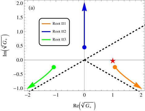
(a)

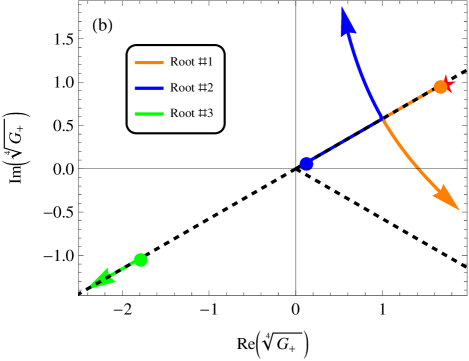
(b)

Figure 5: Trajectories of the three solutions of (LABEL:Complex_Airy_G_equation) for $y_{+}=G_{+}^{\frac{1}{4}}$ and varying $M$. (a) The trajectories for $z=1$. The arrowheads point in the direction the solution moves as $M$ is increased, up to $1000$; the base of the arrow is the value of each root at $M=1$. Note that only one particular root is in the vicinity of $z^{\frac{1}{4}}$ (marked by a red star), tending to it asymptotically if $\left|z\right|$ is increased with $M$ held fixed. As $M$ increases the solutions tend towards the three cubic roots of $C_{3}\left(M\right)/3iM$, which lie on the positive imaginary axis and along the $\pm e^{\mp\frac{i\pi}{6}}$ directions, marked by the dashed lines. Note that the solution of interest (orange) tends to the principal branch of the cubic root, $\sqrt[3]{C_{3}\left(M\right)/3iM}$; this behavior experiences a crossover when transitioning across the Stokes line at $\arg z=\frac{2\pi}{3}$, after which the root which stems from $z^{\frac{1}{4}}$ tends to the imaginary axis, cf. the right panel. (b) The same trajectories for $z=16e^{\frac{2\pi i}{3}}$. Note that initially all roots lie on the line parallel to $e^{\frac{i\pi}{6}}$. The “primary” root coming from $z^{\frac{1}{4}}$ “collides” with the root coming from $0$, after which they become a complex-conjugate pair of solutions for $r=\left(\frac{G}{z}\right)^{\frac{1}{4}}$, and continue to tend to the same asymptotes as before. For $\arg z$ any larger, the asymptotes of these two roots will be swapped.

Let us then explore the behavior of $1-\sqrt{z}/\sqrt{G}$ as a function of $\arg z$. Beginning with real $z$, the resolved trajectories of the three solutions for $G_{+}^{\frac{1}{4}}$ as $M$ is increased are depicted in 5(a)thesubfigure, for $z=1$. Note the structure of the solutions: one imaginary and a pair which is symmetric about the imaginary axis. This is directly deduced by the fact that for real $z$, substituting $y=ix$ into (LABEL:Complex_Airy_G_equation), the resulting equation for $x$ is a cubic equation with strictly real coefficients, so is has one real root and a conjugate pair of complex roots. After rotating back to $y$, we obtain the aforementioned structure.

Next, we observe that indeed one particular root of $G^{\frac{1}{4}}$, that colored orange in 5(a)thesubfigure, tends continuously to $z^{\frac{1}{4}}$ for large $\left|z\right|$. This identifies the root of interest among the three which should be inserted into (LABEL:SCE_Complex_Airy_With_G). Note that as $M\rightarrow\infty$ this root tends to the principal root of $\sqrt[3]{C_{3}\left(M\right)/3iM}$. However, this property is suddenly violated once we cross the Stokes line at $\arg z=\frac{2\pi}{3}$. To see this, we substitute $y=rz^{\frac{1}{4}}$ into (LABEL:Complex_Airy_G_equation) to obtain

$$3\Delta ir(r^{2}-1)z^{\frac{3}{4}}=C_{3}\left(M\right)/M\,.$$ (93)

Examining $z=\left|z\right|e^{\frac{2\pi}{3}i+i\delta\varphi}$ which is close to the Stokes line, we then have

$$r(r^{2}-1)=-\frac{\Delta C_{3}\left(M\right)}{3\left|z^{\frac{3}{4}}\right|M}e^{-\frac{3}{4}i\delta\varphi}\,,$$ (94)

so on the line ($\delta\varphi=0$), the equation for $r$ is also cubic with real coefficients. There are three roots which converge to $r=0,-1$ and $+1$ for large $\left|z\right|$. For $\Delta=+1$, as $M$ is increased, a negative real root $r<-1$ exists, while the roots originating at $0,1$ must eventually reach argument $\pm\frac{\pi}{3}$, as they are the two complex-conjugate cubic roots of $-\frac{C_{3}\left(M\right)}{M}\sim-\sqrt{M}$. Clearly, there is a critical value $M\left(z\right)$ where these two roots meet on the real line before jumping off it and becoming a conjugate pair. Since the roots meet, it is ill-defined to ask to which side of the line the root originally at $r=1$ scatters; the collision mixes their identity. See 5(b)thesubfigure for details. The point at which this collision occurs can be found by equating the discriminant of (LABEL:Airy_equation_scatter_on_2pi3_line) to zero with $\delta\varphi=0$, yielding

$$\sqrt{\frac{4}{3}}\left|z\right|^{\frac{3}{4}}=\frac{C_{3}\left(M\right)}{M}\sim\sqrt{M}\,.$$ (95)

If $z^{\frac{1}{4}}$ is slightly below the line $e^{+\frac{i\pi}{6}}$(i.e. $\delta\varphi=\epsilon<0$), then this symmetry is broken, and the solution $r=1$ is “scattered” below $r=0$, tending to the line $e^{-\frac{i\pi}{3}}$, so $G_{+}^{\frac{1}{4}}$ tends to $e^{-\frac{i\pi}{3}+\frac{1}{4}\frac{2\pi i}{3}}=e^{-\frac{i\pi}{6}}$. This is the case which happens with real and positive $z$. If instead $\delta\varphi>0$, then our privileged root scatters from $r=1$ up to $r\propto e^{+\frac{i\pi}{3}}$ and $G_{+}^{\frac{1}{4}}$ tends to the line $e^{+\frac{i\pi}{3}+\frac{1}{4}\frac{2\pi i}{3}}=e^{+\frac{i\pi}{2}}$. The same logic applies for the root $G_{-}$, with all the signs of the arguments above negated.

We now come to the following interpretation of the behavior of the Airy SCE as the argument of $z$ is increased: Either one of the $z$-continuous roots of $G_{+}^{\frac{1}{4}}$ or $G_{-}^{\frac{1}{4}}$ tends from $z^{\frac{1}{4}}$ to the imaginary line as $N$ (and consequently $M$) is increased. Note that when deriving the SCE for $\tilde{\mathrm{Ai}}$, we had assumed $\arg G\neq\pi$, so that $\mathrm{Re}\sqrt{G}>0$ and the integral $\int e^{-\sqrt{G}t^{2}}dt$ converged. This implied that the arguments of the quartic roots $G^{\frac{1}{4}}$ must be in the range $\left[-\frac{\pi}{4},\frac{\pi}{4}\right]$. However, as the argument of one of the roots now tends from $\arg z$ to $\pm\frac{\pi}{2}$, it at one point leaves this range and renders our assumption wrong, and the Gaussian identities that we had used are invalid. Conceptually, looking back to the original integral, now $\mathrm{Re}\sqrt{G}<0$ so one may argue that the Gaussian weight $e^{-\sqrt{G}t^{2}}$amplifies the $t^{3}$ perturbations which is dominant far from from the origin, contrapuntal to our perturbative approach. The only remedy to this situation is to replace the offending root with another solution of (LABEL:Complex_Airy_G_equation) which is contained inside the $\pm\frac{\pi}{4}$ phase cone. For $G_{\pm}^{\frac{1}{4}}$, this is the root whose argument approaches $\mp\frac{i\pi}{6}$. This means that the SCE cannot reconcile two conflicting goals: self-consistently eliminating first order corrections, and reproducing the original integral representation at the low-$N$\large-$z$ limit. This is similar to the incompatibility observed in the discussion of the double-well case in V.

Now that a single limit is chosen for $G_{\pm}$, we can analyze the behavior of the factor of $1-\sqrt{z}/\sqrt{G}$, and its impact on the SCE accuracy, when $M\rightarrow\infty$. These are demonstrated in Figs. 6(a)thesubfigure and 6(b)thesubfigure, respectively.

Recalling that $C_{3}\left(M\right)/3M\sim\sqrt{M}$, it asymptotically behaves as

$$\left(1-\frac{\sqrt{z}}{\sqrt{G_{\Delta}}}\right)^{N}\sim\left(1-\frac{\sqrt{z}}{M^{\frac{1}{3}}3^{-\frac{2}{3}}e^{-\frac{\Delta}{3}\pi i}}\right)^{N}\sim e^{-\left(\frac{9}{\alpha}\right)^{\frac{1}{3}}e^{\frac{\Delta}{3}\pi i}\sqrt{z}N^{\frac{2}{3}}}\,,$$ (96)

giving us again a stretched exponent. This factor is convergent only if $\mathrm{Re}\left\{e^{\frac{\Delta}{3}\pi i}\sqrt{z}\right\}>0$, or if $\left|\frac{\varphi}{2}+\Delta\frac{\pi}{3}\right|<\frac{\pi}{2}$, with $\varphi=\arg z$. This would imply that the factors $1-\sqrt{z}/\sqrt{G_{\pm}}$, which clearly approach $1$ as $M\rightarrow\infty$, do so from within the unit circle in the complex plane. To satisfy this simultaneously for both $\Delta=\pm 1$, we require that $\left|\varphi\right|<\frac{\pi}{3}$, revealing the other Stokes line of the Airy function. For larger arguments, this factor approach $1$ from outside the circle, and competes against the exponentially convergent series coefficients. However, we note a difference between the two stokes wedges:

For $\frac{\pi}{3}<\left|\varphi\right|<\frac{2\pi}{3}$ and large $z$ (small $M$), $\sqrt{G}$ originate in the vicinity of $\sqrt{z}$, and this $1-\sqrt{z}/\sqrt{G}$ starts close to zero. This implies that it steadily grows in magnitude as $M$ increases, eventually protruding out of the unit circle, after which it reaches some maximal magnitude greater than unity, and then starts approaching $1$ from outside. However, this maximal magnitude is bounded by its value for $\varphi=\pm\frac{2\pi}{3}$. Substituting (LABEL:Airy_M_Scatter_point) back into (LABEL:Airy_equation_scatter_on_2pi3_line), we find that at the collision $r=3^{-\frac{1}{2}}$, or $\sqrt{G_{+}}=\sqrt{z}/3$, so that at this point $\left(1-\sqrt{z}/\sqrt{G_{+}}\right)^{N}=\left(-2\right)^{N}$ universally for all $\left|z\right|$. Consulting 1, note that the convergent coefficients are bounded by $10^{-0.305N}\approx 2.02^{-N}$, so the error of the expansion at the collision (the cusp visible in 6(b)thesubfigure) is bounded by $(2/2.02)^{N}\approx 10^{-0.004N}$. However, the actual exponential convergence rate is roughly $10^{-0.5N}$, so the scaling of the cusp is closer to $10^{-0.20N}$, or $10^{-0.27\left|z\right|^{\frac{3}{2}}}$ if we substitute $N=M/\alpha$, with $M$ given approximately by (LABEL:Airy_M_Scatter_point), and $\alpha=\alpha^{*}\approx 1$. This implies that the exponential convergence is always dominant in this sector, regardless of $\left|z\right|$.

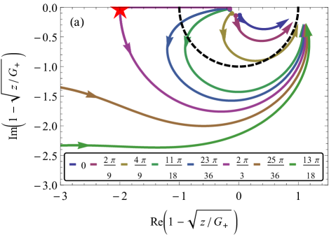
(a)

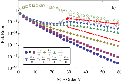
(b)

Figure 6: Behavior of the SCE in the complex plane, for fixed $\left|z\right|$ and varying $\arg z$. (a) Trajectories of the factor $1-\sqrt{z}/\sqrt{G_{+}}$, as $M$ is increased up to $10^{4}$, for the listed values of $\arg z$ and $\left|z\right|=8$. The unit circle is plotted for reference. As the argument of $z$ is increased, the trajectories sweep outwards. For $\left|\arg z\right|<\frac{\pi}{3}$, the trajectories are contained inside the unit circle. For $\frac{\pi}{3}<\left|\arg z\right|<\frac{2\pi}{3}$, they exit it and eventually converge to $+1$ from outside. However, the closer $\arg z$ is to $\frac{2\pi}{3}$, the “sharper” the angle of protrusion through the circle, and the further outside the trajectory reaches before attaining its maximal magnitude. At $\arg z=\frac{2\pi}{3}$, the trajectory heads radially outwards on the negative real axis before turning sharply (red star) at $\left(-2\right)$, a value independent of $\left|z\right|$ which corresponds to the scattering point visible in 5(b)thesubfigure. This sharp turn occurs at $M\approx 28.09$, as predicted by (LABEL:Airy_M_Scatter_point) for $\left|z\right|=8$. This point corresponds to the cusp in the right panel (red star). Lastly, for $\left|\arg z\right|>\frac{2\pi}{3}$, the origins of the trajectories jump abruptly to far away from the unit circle. Another arrowhead was placed on the points corresponding to $M=30$ for reference; for any larger $M$, the trajectories are continuous as a function of $\arg z$. (b) The relative error of the SCE versus the order $N$ for the same values of $z$ as in the left panel, with $M\left(N\right)=N$. For all arguments under $\frac{2\pi}{3}$, the error is roughly identical until order $\sim 10$, at which point the convergence rate is slowed down with increasing phase. As the argument is increased towards $\frac{2\pi}{3}$, a local bump in the error forms. For $\mbox{$\arg$}z=\frac{2\pi}{3}$, a cusp occurs at $N=29$ (red star). This is the first integer value of $N$ for which $M$$\left(N\right)$ is greater than the value at which the collision in 5(b)thesubfigure occurs, corresponding to the red star in the left panel. After this bump, the expansion returns to converge exponentially for all $\arg z$. The errors for $\arg z>\frac{2\pi}{3}$ exhibit the diverging nature of the Airy SCE in this Stokes wedge at low orders, but eventually the SCE starts to converge for sufficiently large $N$. Note the eye formed for $N<30$; for $N>30$, the error transitions smoothly across both Stokes lines, showing that the SCE smooths out the Stokes lines at large order. Lastly, the lower and upper dashed lines represent the uniform exponential convergence component in the $\left|\arg z\right|<\frac{\pi}{3}$ and $\frac{\pi}{3}<\left|\arg z\right|<\frac{2\pi}{3}$ Stokes sectors, respectively. The lower line was obtained by fitting an exponential profile to the SCE of $\mathrm{Ai}\left(0\right)$, which does not exhibit a stretched-exponential component (cf. 7). This line bounds the error for all $\left|\arg z\right|<\frac{\pi}{3}$, while for $\frac{\pi}{3}<\left|\arg z\right|<\frac{2\pi}{3}$, the error will eventually exceed it once the corresponding trajectory leaves the unit circle; for example, the yellow diamonds with $\arg z=\frac{4\pi}{9}$ cross this line at order $N\approx 200$. The upper dashed line was obtained by multiplying the lower line by $2^{N}$, as a bound on the factor $\left(1-\sqrt{z}/\sqrt{G_{+}}\right)^{N}$ in the $\frac{\pi}{3}<\left|\arg z\right|<\frac{2\pi}{3}$ wedge. Note that to a good approximation, the cusp lies on this line (cf. the left panel).

In stark contrast, for $\frac{2\pi}{3}<\left|\varphi\right|<\pi$, $\sqrt{G}$ originates near zero and so the factor $1-\sqrt{z}/\sqrt{G}$ is very large for small $M$, before it tends to $1$ at large order. The larger $\left|z\right|$, the more egregious this problem becomes. This is essentially an extension to the complex plane of the situation observed in (LABEL:Double_Well_G): Once again, the SCE cannot simultaneously reconcile both the demand for self-consistency of $\left\langle t^{2M}\right\rangle$ and the limit of $G\rightarrow z$. Thus, we expect that for $\frac{2\pi}{3}<\left|\varphi\right|<\pi$, the SCE starts by diverging for small $N$. At larger orders, the stretched-exponential behavior of (LABEL:Airy_stretched_exponent) is recovered, which competes against the convergent coefficients, and the exponential convergence becomes dominant (i.e., the error becomes monotonically decreasing thereafter) at order $N\sim\left|z\right|^{\frac{3}{2}}$.

Lastly, since we picked a consistent large-$M$ limit for $G_{\pm}$, we note this implies that at sufficiently large order, the SCE transitions smoothly across the $\varphi=\pm\frac{2\pi}{3}$ Stokes line. This is because at $N\rightarrow\infty$, the factors $\left(1-\sqrt{z}/\sqrt{G}\right)^{N}$ are continuous as a function of $z$, producing the stretched exponent in (LABEL:Airy_stretched_exponent) which is entire. It is only once $N$ is reduced, that the roots split discontinuously, with $\sqrt{G}\rightarrow\sqrt{z}$ or $\sqrt{G}\rightarrow 0$, depending on whether $\arg z$ is larger or smaller than $\frac{2\pi}{3}$. This occurs abruptly, at the value of $N$ at which the “collision event” depicted in 5(b)thesubfigure takes place, and predicted by (LABEL:Airy_M_Scatter_point) to be at $N=\frac{1}{\alpha}\times\frac{4}{3}\left|z\right|^{\frac{3}{2}}$. Of course, the Airy function is smooth across the lines, and it was also shown Berry (1989a, b); Olver (1990) that the usual asymptotic expansion is smooth if sufficiently magnified. In Ref. Berry (1989a), this smoothing is attained by truncating the series at its least term, which occurs at $N=\frac{4}{3}\left|z\right|^{\frac{3}{2}}$ (given by the large-$n$ summand in (LABEL:Airy_tilde_standard_asymptotic_form), or by the difference between the exponents in the two saddles mentioned above, $\pm\frac{3}{2}z^{\frac{3}{2}}$, as prescribed by Berry and Howls (1991)). This implies that by increasing the ratio $\alpha$, the SCE can provide a smooth approximation faster than the standard asymptotic expansion.

To summarize, we find the following behavior of the SCE, based on the location of $z$ with respect to the Stokes lines of the Airy function:

(i) For $\left|\arg z\right|<\frac{\pi}{3}$, the SCE correctly captures the behavior of $\mathrm{Ai}\left(z\right)$ at any order if $M=\alpha N$ is chosen appropriately. Convergence is exponential and uniform, with a rate bounded by $10^{-0.305N}$ [cf. 1], and supplemented by a convergent $z$-dependent stretched-exponential $\left|1-\sqrt{z}/\sqrt{G}\right|^{N}\sim\exp\left\{-\mathrm{Re}\left(3^{2/3}\alpha^{-1/3}e^{i\pi/3}z^{1/2}N^{2/3}\right)\right\}$ [cf. (LABEL:Airy_stretched_exponent)].

(ii) For $\frac{\pi}{3}\leq\left|\arg z\right|\leq\frac{2\pi}{3}$, SCE provides better approximations with increasing $N$ from as soon as $N=0$, but the rate of convergence is diminished once $1-\sqrt{z}/\sqrt{G}$ exits the unit circle. If this protrusion is at a sharp angle, then the error experiences a bump. However for any $z$, it may be bounded by $\left|1-\sqrt{z}/\sqrt{G}\right|^{N}<2^{N}\approx 10^{0.30N}$ [see 6(a)thesubfigure], which is weaker than the exponentially convergent component (both its bound and its rate in practice), and convergence is formally still uniform.

(iii) For $\frac{2\pi}{3}<\left|\arg z\right|\leq\pi$, SCE produces an initially increasing error at leading orders due to a very large $\left|1-\sqrt{z}/\sqrt{G}\right|^{N}$, but once a critical order $N_{c}\left(z\right)$ is surpassed, after which the exponentially-convergent coefficients become dominant, the SCE is again convergent. $N_{c}$ is monotonic in $\left|\arg z\right|$ and scales as $\sim\left|z\right|^{\frac{3}{2}}$, as implied by (LABEL:Airy_stretched_exponent).

(iv) At large enough order, the SCE is smoothed, and varies continuously between the three regimes above. This occurs once $M\left(N\right)=\frac{4}{3}\left|z\right|^{\frac{3}{2}},$ analogous to the least-term Stokes smoothing at $N=\frac{4}{3}\left|z\right|^{\frac{3}{2}}$ of traditional asymptotics.

All four regimes are depicted in 6(b)thesubfigure. The smoothing and subsequent exponential convergence at sufficiently large order imply that the SCE converges uniformly on any disk of finite radius in the complex plane, i.e. for $\left|z\right|\leq R<\infty$. Due to the duality $g\Leftrightarrow z^{-\frac{3}{4}}$, this corresponds the to the uniform convergence of the double-well SCE for any finite $g\geq\epsilon>0$ in V.

VII.3 Further Numerical Results

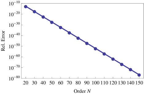
Figure 7: Convergence of the SCE to $\mathrm{Ai}\left(0\right)$. Shown is the relative error of the expansion (dots) versus the order $N$, along with an exponential fit, $R^{\left(N\right)}=10^{B-AN}$ (solid line). We evaluate the series with $M=N$. The fitted value for $A$ is $0.492$, showing that the SCE recovers another significant digit of $\mathrm{Ai}\left(0\right)$ every other order, greatly exceeding the convergence rate estimated in 1 for $q=3$.

Recalling that $z=0$ corresponds to an infinite anharmonicity [cf. the rhs of (LABEL:Airy_representation_integral_cosine)], and so represents an extreme test case, we first examine the convergence of the SCE to $\mathrm{Ai}\left(0\right)$. We take $z=0$ as having phase zero, that is, lying on the positive real line, and so it is contained in the first Stokes wedge. In fact, evaluating the expansion at $z=0$ allows us to isolate the uniform exponential convergence rate without the additional stretched-exponential component, since $\left(1-\sqrt{z}/\sqrt{G_{\pm}}\right)^{N}=1$ identically. This is shown in 7. Remarkably, while the SCE is formulated around large $\left|z\right|$, it produces a convergent sum even at $z=0$, while the comparable asymptotic expansion (LABEL:Airy_tilde_standard_asymptotic_form) has a convergence radius of zero. The relative error of the expansion is fitted with an exponential trend $\log_{10}R^{\left(N\right)}=B-AN$, reaching a minimal $\chi^{2}=0.03$ for the values $A=0.492$ and $B=-2.85$. This implies that SCE reproduces a significant digit of $\mathrm{Ai}\left(0\right)$ every two orders. Furthermore, this rate is then assisted by a convergent stretched-exponent in the first Stokes wedge, $\left|\arg z\right|<\frac{\pi}{3}$.

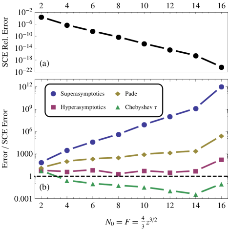
Figure 8: Comparison of the Airy SCE with other asymptotic methods. (a) The relative error of the Airy SCE. The horizontal axis is the singulant $F=\frac{4}{3}z^{\frac{3}{2}}$, and at each point the SCE is evaluated to order $N_{0}=F$, which is the same truncation as the superasymptotic scheme. The solid lines are a guide to the eye. (b) The errors produced by superasymptotics, hyperasymptotics, Padé approximants and the $\tau$ method, relative to that produced by the SCE (i.e., the data was normalized by that shown in the top panel). The solid lines are a guide to the eye. Evaluated at the same order, the SCE consistently outperforms superasymptotics and the Padé approximants, and again produces an error very similar to hyperasymptotics (cf. 2 and subsequent discussion), although the hyperasymptotic series is formally of order $2N_{0}$. The Chebyshev $\tau$ method appears to give a few additional significant digits, but the SCE again converges faster in the large-$N$ limit — this is demonstrated in 9(b)thesubfigure.

Let us again compare the SCE against the methods of Competing_Methods. The numerical evaluation of the SCE versus super and hyperasymptotics, as well as the Padé and $\tau$ approximations, is depicted in 8. All methods are evaluated at the same order as the superasymptotic least-term truncation $N_{0}=\frac{4}{3}z^{\frac{3}{2}}$, and the hyperasymptotic trans-series is evaluated up to level three, or less if it terminates earlier. Similarly to IV, the SCE exhibits performance much better then superasymptotics, and comparable with hyperasymptotics, though in principle the hyperasymptotic expansion is of order $2N_{0}$.

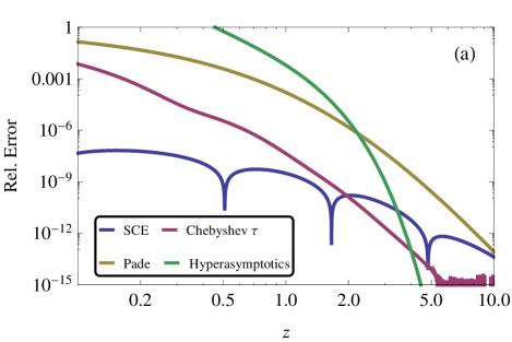
(a)

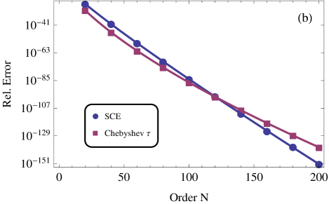
(b)

Figure 9: Comparison of the Airy SCE versus the Padé and Chebyshev $\tau$ approximations (a) The relative accuracy of the three methods as a function of $z$. All are evaluated at fixed order $N=7$. Also plotted is the estimated best achievable hyperasymptotic error, as predicted by (LABEL:Airy_Hyperasymptotic_Error_Bound). By construction, the hyperasymptotic approximation order is $2N_{0}=2\times\frac{4}{3}z^{\frac{3}{2}}$, which gives $2N_{0}=7$ at $z\approx 1.9$. Much like the anharmonic case, SCE dominates the other methods for “stronger” couplings — this time, at smaller $z$. The noise seen near $z=10$ in the $\tau$ method is numerical noise due to evaluation at machine precision. The sharp dips in the SCE error are points where the error switches signs, i.e. points where $\mathrm{Ai}^{\left(N\right)}\left(z\right)$ and $\mathrm{Ai}\left(z\right)$ intersect. (b) The relative error of the SCE and the Lanczos Chebyshev $\tau$ method versus $N$, for $z=8$. As before (cf. 3(b)thesubfigure), the SCE surpasses the $\tau$ method for sufficiently large $N$. Both methods were fitted with trend lines of the form $10^{C-AN-BN^{\frac{2}{3}}}$. The SCE yields the values $A=0.492$ and $B=1.446$, greatly exceeding our minimal bounds of uniform $A=0.305$ and $z$-dependent $B=1.28$. The $\tau$ method yields a negligible $A=0.007$, suggesting that it only contains the $10^{-BN^{\frac{2}{3}}}$ component, with $B=4.00$.

The SCE is compared more directly with the Padé and $\tau$ schemes in 9(a)thesubfigure, where they are all evaluated at fixed order $N=7$. The SCE is consistently more accurate than the Padé approximants, and overtakes the Chebyshev $\tau$ method for stronger non-linearities (smaller $z$). We again find that even for larger $z$ the SCE is more rapidly convergent than the Chebyshev $\tau$ method, as shown in 9(b)thesubfigure.

VIII Extension to Multiple Degrees of Freedom

In the case of an oscillator in more than one spatial dimension, or alternatively that of several coupled oscillators, we may examine a potential of the generic form

$$V\left(\left\{x_{i}\right\}\right)=\frac{1}{2}\sum\gamma_{ij}x_{i}x_{j}+\sum g_{ijkl}x_{i}x_{j}x_{k}x_{l}\,,$$ (97)

for which we assume that $\gamma_{ij}$ is a positive definite quadratic form and $g_{ijkl}$ is a non-negative form, and each coordinate $\left\{x_{i}\right\}_{i=1}^{D}$ takes values on the entire real line. The total partition function for the system would be

$$\Xi=\int_{-\infty}^{\infty}\prod_{i=1}^{D}dx_{i}e^{-\beta\left(\frac{1}{2}\sum\gamma_{ij}x_{i}x_{j}+\sum g_{ijkl}x_{i}x_{j}x_{k}x_{l}\right)}\,.$$ (98)

However, we may transform this integral to radial and angular coordinates in the $D$-dimensional $x$-space, to get

$$\Xi =\int d^{D-1}\Omega\int_{0}^{\infty}dr\,r^{D-1}e^{-\beta\left(\frac{1}{2}\gamma\left(\Omega\right)r^{2}+g\left(\Omega\right)r^{4}\right)}$$

$$=\int d^{D-1}\Omega\left(\beta\gamma\left(\Omega\right)\right)^{-\frac{D}{2}}\mathcal{Z}_{D-1}\left(\frac{g\left(\Omega\right)}{\beta\gamma^{2}\left(\Omega\right)}\right)\,,$$ (99)

with $\Omega$ representing all the angular dependencies, and $\mathcal{Z}_{D-1}$ defined similarly to $\mathcal{Z}$ in (LABEL:Z_definition), apart from the change of integration limit and measure by $\int_{-\infty}^{\infty}dx\rightarrow\int_{0}^{\infty}x^{D-1}dx$. $\gamma\left(\Omega\right)$ and $g\left(\Omega\right)$ are the quadratic and quartic coefficients of the potential along the ray defined by $\Omega$, which by assumption are positive and non-negative, respectively. By satisfying first-order self-consistency for $\left\langle r^{2M}\right\rangle$, we find that

$$\mathcal{Z}_{D}^{\left(N\right)}\left(g\right)=\frac{1}{2}\left(\frac{2}{G}\right)^{\frac{D+1}{2}}\sum_{n=0}^{N}\left[1-\frac{1}{G}\right]^{n}\sum_{l=0}^{n}\binom{n}{l}\left(-1\right)^{l}\frac{\Gamma\left(n+l+\frac{D+1}{2}\right)}{n!\left(M+D+2\right)^{l}}\,,$$ (100)

and the SCE of the partition function is

$$\Xi^{\left(N\right)}=\int d^{D-1}\Omega\left(\beta\gamma\left(\Omega\right)\right)^{-\frac{D}{2}}\mathcal{Z}_{D-1}^{\left(N\right)}\left(\frac{g\left(\Omega\right)}{\beta\gamma^{2}\left(\Omega\right)}\right)\,.$$ (101)

For finite $D$ (i.e., $D$ which does not scale with $N$), the convergence of the expansion will not be adversely impacted by the additional $D$-dependent factors. In particular, if the SCE parameter $M$ is chosen such that $\mathcal{Z}_{D}^{\left(N\right)}$ is exponentially convergent (e.g., $M+D=\alpha N$), then the angular integration in (LABEL:many_body_SCE) adds a numeric factor which depends on $D$, but the error would still be exponentially decaying in $N$ for any strength of the anharmonicity. Indeed, the numerically efficacy of a similar scheme was recently demonstrated without proof for the $O\left(n\right)$ model in zero dimensions Rosa et al. (2016).

The case of many-body problems (i.e., $D\gg 1$) requires greater care, as we expect that the rate of convergence of the expansion with $N$ would depend on $D$. We leave this subject for future work.

IX Conclusions and Outlook

In this paper we have investigated the analytical properties of the SCE by applying it to the toy model of the classical anharmonic oscillator in thermal equilibrium. We utilized the benefit of an explicit closed-form expansion to show that for this model the SCE is exponentially and uniformly convergent for any positive power $q$ and strength $g$ of the anharmonicity $gx^{q}$, compared with standard perturbation theory which is rapidly divergent and must rely on resummation. We put analytical bounds on the remainder of the expansion at any given order, allowing us to identify the space of expansion parameters that guarantees convergence. Remarkably, we argued that the expansion remains (non-uniformly) convergent for double-well (negative quadratic coupling) potentials, even if it is not performed about the double-well minima, but rather around a harmonic reference. We also provide an estimate for the optimal choice of a self-consistent quadratic coupling, and the minimal rate of convergence obtained for this value. Lastly, we briefly explored the complex-plane behavior of the SCE by applying it to the Airy function $\mathrm{Ai}\left(z\right)$, where we have seen the effect of the Airy function’s Stokes lines, and their expected smoothing at large order. In both cases, the SCE compares favorably against other numerical and asymptotic methods, most strikingly in the strong-coupling regime. We have also shown that convergence carries over to any arbitrary finite number of coupled oscillators.

Due to its convergence for any $q$, we expect that the SCE should still be convergent for any analytic perturbing potential $gV\left(x\right)$ which scales polynomially at infinity. It can then be shown that an $x^{2M}$-consistent SCE is only an implicit function of $g$, depending explicitly only on $G\left(M,g\right)$. The large-order convergence rate would then be determined by the asymptotic scaling of $V\left(x\right)$ for $x\rightarrow\infty$. We concede that for all but the simplest systems, obtaining corrections beyond the first few leading terms is impractical; despite this fact, we believe that we have demonstrated the appeal of SCE even at low orders, with its superb numerical accuracy at small $g$ and improved behavior at large $g$.

We have also elucidated the relationship between the SCE and related variational schemes, such as ODM, OPT, and LDE. In particular, we have observed the equivalence between the scaling of $G\left(N\right)$ in the SCE with that given by the PMS and FAC conditions. However, the SCE offers a few advantages: (i) The PMS or FAC criteria might not be solvable exactly, most notably at high order; furthermore, it is non-trivial that either of them has a unique solution for $G\left(N\right)$, or any at all (for example, in Ref. Buckley et al. (1993) the PMS condition has no solution for $N$ even, despite the fact that the approximation is optimal for even $N$, as shown in 1(a)thesubfigure). The SCE condition, which is always first order, is easily implemented and solved. (ii) The SCE condition is physically motivated, allows desired physical features to be built-in into the approximation, and permits flexibility in the formulation of the expansion, such as in the choice of conserved observables. Its strength is exemplified by the remarkable result that in the SCE, optimal convergence is achieved repeatedly in the linear scaling $M\left(N\right)\sim N$, for any possible anharmonicity.

These results provide fertile grounds for additional inquiry: We have seen that for a given system, the SCE is not unique — neither the exact scheme of the expansion nor the selection of the self-consistent parameters are such. Is there any physical significance to preserving the spatial moments $x^{2M}$? If so, then one would require an a priori method of estimating a suitable choice for $M$ (or perhaps even $G\left(M\right)$ directly) when the self-consistency criteria cannot be evaluated explicitly. If not, are there other observables that would yield better results? A deeper question is whether the values of $\alpha$ found above are universal, depending only on the scaling of $V\left(x\right)$ for large $x$; for example, repeating the calculations for a $d$-dimensional isotropic oscillator with $r^{q}$ anharmonicities would produce the same values.

The next logical extensions to the method are apparent: One is an expansion in many mutually-coupled degrees of freedom, up to the thermodynamic limit, in which an expansion of intensive quantities, instead of the macroscopic partition function, may be preferable. Another is investigating the SCE of the quantum anharmonic oscillator, for which expanding the partition function is easiest in the imaginary-time path integral formulation, making it equivalent to a 1D classical string. This immediately raises additional ambiguities in the scheme: The choice of basis for the path-integral (i.e., spatial vs. coherent representation); the addition of a modified mass as another self-consistent parameter; and an extended selection of observables to optimize, such as $\hat{x}^{2M}$, $\hat{p}^{2M}$, and $\hat{\mathcal{H}}_{0,1}^{2M}$, most of which were equivalent in the classical case, up to a redefinition of $M$. However, in the high-temperature limit, all these schemes should reduce to the same classical results presented here. In particular, since the SCE could be formulated for any temperature, it might bridge the regimes of zero and finite $T$, whose connection was not apparent in previous treatments of the problem Bender et al. (1994); Arvanitis et al. (1995). Ideally, a combination of both extensions will allow the application of the SCE to various field-theoretical models. Given the success of low-order SCE or the related methods (ODM, OPT, and LDE) for such systems Schwartz and Edwards (2002); Edwards and Schwartz (2002); Li et al. (1996); Mattingly and Stevenson (1994); Stevenson (2013); Abdalla et al. (2009); Kneur et al. (2007, 2010); Braaten and Radescu (2002); Yukalov (1985); Yamada (2007); Kneur et al. (2003); de Souza Cruz et al. (2001); Rosa et al. (2016), the prospects for this seem promising.

Or course, the notion of modifying the studied physical system to mitigate divergences is nothing new. Examples are the masking of a bare mass by renormalization Peskin and Schroder (1995), or the shift of the oscillation frequency in secular perturbation theory Strogatz (1994). While conceptually distinct, in the sense that it removes a series divergence instead of reining in isolated terms, we would like to see if the SCE, when applied in these contexts, might shed new light on these methods.

Lastly, similar approaches of expansion about a shifted zeroth-order system were used for related purposes, such as ensuring the convergence of the resulting PT Turbiner (1984, 2005). Most recently, Serone, Spada, and Villadoro introduced Exact Perturbation Theory (EPT) Serone et al. (2017a, b) an approach in which the problem is framed as a particular realization in the parameter space of a more general model with a Borel-resummable PT, and the coupling-dependent interpolation within this space provides the non-perturbative contributions. This is comparable to the SCE parameter $G$, whose $g$ dependence encodes into the expansion information which is non-perturbative in $g$. However, as this technique relies on the underlying resummability of the interpolated model, it requires knowledge of the large-order terms of its PT, whereas the SCE provides a convergent sequence of approximations. Furthermore, the formulation of such an EPT is limited by the availability of a resummable analogue, which is much more restrictive than the flexibility afforded by the SCE. Nevertheless, these approaches might have a deeper connection with the SCE. Indeed, the asymptotic nature of PT is well understood, providing physical insights such as tunneling and instantons Zinn-Justin (2002), resurgent trans-series Cherman et al. (2015), and so forth. It yet remains to be seen how these reflect in the analytical structure of the SCE, which we hope will become clearer in future work.

We thank Michael V. Berry, Leonid I. Glazman, Eytan Katzav, Michael Kroyter, and Moshe Schwartz for very helpful discussions. Support from the Israeli Science Foundation (grant number 227/15), the Israel Ministry of Science and Technology (under contract number 3-12419), the German-Israeli Science Foundation (grant I-1259-303.10/2014), and the US-Israel Binational Science Foundation (grants 2014262 and 2016224), is gratefully acknowledged.

Appendix A Direct Estimation of the Quartic SCE Coefficients

The specific case of the quartic anharmonicity admits a direct error estimation by inspection of the SCE series coefficients. Given by the sum over $l$ in (LABEL:SCE_partition), these coefficients may be expressed as

$$S_{n,K} =\sum_{l=0}^{n}\binom{n}{l}\frac{\Gamma\left(n+l+\frac{1}{2}\right)}{n!\left(-K\right)^{l}}=\frac{\left(-1\right)^{n}\pi}{K^{n}n!\Gamma\left(\frac{1}{2}-2n\right)}{}_{1}F_{1}\left(-n,\frac{1}{2}-2n;-K\right)\,,$$ (102)

where ${}_{1}F_{1}\left(a,b;z\right)$ is Kummer’s confluent hypergeometric function (DLMF, , Chap. 13). Note that when the parameter $a$ is a negative integer, this is a finite-order polynomial in $z$. As this is an alternating polynomial in the variable $K$, it is difficult to estimate directly; delicate cancellations occur between terms of similar magnitude and opposite sign. However, we may remedy this situation by utilizing Kummer’s transformation rule (DLMF, , Eq. (13.2.39)),

$${}_{1}F_{1}\left(a,b;z\right)=e^{z}{}_{1}F_{1}\left(b-a,b;-z\right)\,,$$ (103)

so we find

$$S_{n,K}=\frac{\left(-1\right)^{n}\pi e^{-K}}{K^{n}n!\Gamma\left(\frac{1}{2}-2n\right)}{}_{1}F_{1}\left(\frac{1}{2}-n,\frac{1}{2}-2n;+K\right)\,.$$ (104)

This, however, comes at a cost: since now the parameter $a$ is not a negative integer, this hypergeometric function constitutes an infinite series. Despite this, it is useful to note that for $a$ that is not a negative integer, we have an asymptotic expansion for large arguments (DLMF, , Eq. (13.2.23)),

$${}_{1}F_{1}\left(a,b;z\rightarrow\infty\right)\sim\frac{\Gamma(b)}{\Gamma\left(a\right)}e^{z}z^{a-b}\,,$$ (105)

so for very large $K\gg n$, we get the leading order behavior

$$S_{n,K}\sim\frac{\left(-1\right)^{n}\pi}{\Gamma\left(\frac{1}{2}-n\right)n!}=\frac{\Gamma\left(n+\frac{1}{2}\right)}{n!},$$ (106)

where we have used the reflection property of the gamma function. This reproduces the bounding form we used to prove case 3 of Proposition 1 at the end of III.

Writing down the sum represented by ${}_{1}F_{1}$ explicitly, we have

$$S_{n,K} =\frac{\left(-1\right)^{n}\pi e^{-K}}{K^{n}n!\Gamma\left(\frac{1}{2}-n\right)}\sum_{s=0}^{\infty}\frac{K^{s}\Gamma\left(-n+s+\frac{1}{2}\right)}{s!\Gamma\left(-2n+s+\frac{1}{2}\right)}=\frac{\left(-1\right)^{n}\Gamma\left(n+\frac{1}{2}\right)}{K^{n}n!e^{K}}\sum_{s=0}^{\infty}\frac{K^{s}\Gamma\left(2n-s+\frac{1}{2}\right)}{s!\Gamma\left(n-s+\frac{1}{2}\right)},$$ (107)

again by the reflection property. Note the sign of the terms entering the sum as $s$ is increased: Starting from $s=0$, we start with an initial sign of $\left(-1\right)^{n}$ which holds steady, as all other factors are positive. Beginning at $s=n+1$, the gamma function in the denominator starts alternating signs at every increment of $s$. Lastly, after $s=2n+1$, the gamma function in the numerator also starts alternating signs, thus canceling the sign oscillations in the denominator. In total, exactly $n$ sign flips occur — meaning that for all $s>2n+1$, the terms are strictly positive.

Also note that the magnitude of the ratio of gamma functions attains a minimum at $s\sim\frac{3n}{2}$, since by reflection this ratio can be expressed as $\sim\Gamma\left(\frac{1}{2}+\frac{n}{2}-\left(s-\frac{3n}{2}\right)\right)\times\Gamma\left(\frac{1}{2}+\frac{n}{2}+\left(s-\frac{3n}{2}\right)\right)$. This ratio diverges symmetrically about this point. The factor $\frac{K^{s}}{s!}$, however, is peaked at some finite $s$ and attenuates the gamma ratio for $s\rightarrow 0,\infty$. Thus, we claim that the summand above has two peaks. They occur for integer values of $s$ which are closest to the two solutions of

$$\frac{K\left(n-s-\frac{1}{2}\right)}{\left(s+1\right)\left(2n-s-\frac{1}{2}\right)}=1\,,$$ (108)

which are given by

$$s_{max}^{\pm} =\frac{1}{4}\left[\left(4n+1\right)+\left(2K-1\right)-3\pm\sqrt{\left(4n+1\right)^{2}+\left(2K-1\right)^{2}-1}\right]\approx n+\frac{K}{2}\pm\sqrt{n^{2}+\left(\frac{K}{2}\right)^{2}}\,.$$ (109)

Note that $s_{max}^{-}<n$ and $s_{max}^{{}_{+}}>2n$, so they are both outside the interval of alternating signs. Since the peaks are very narrow (as the summand depends on $s$ exponentially, due to all the gamma functions), we may approximate the total summation by the contribution of the summand only at the two peak indices, giving us

$$S_{n,K}\approx P_{+}+\left(-1\right)^{n}P_{-}\,,$$ (110)

with

$$P_{\pm}=\frac{\Gamma\left(n+\frac{1}{2}\right)}{K^{n}n!e^{K}}\frac{K^{s_{max}^{\pm}}\Gamma\left(+\frac{n}{2}\mp\left(s_{max}^{\pm}-\frac{3n}{2}\right)\right)}{s_{max}^{\pm}!\Gamma\left(-\frac{n}{2}\mp\left(s_{max}^{\pm}-\frac{3n}{2}\right)\right)}\,,$$ (111)

and where we have used the reflection property of the gamma function so that its arguments are positive for both sign cases.

Since the SCE in (LABEL:SCE_partition) is a power series in $\left(1-1/G\right)$, we argue that its remainder should be on the order of the last term in the sum. Let us then specifically examine the last coefficient, $S_{N,K}$. Recalling that $K=M+2$ and substituting $M=\alpha N$ into the approximate roots in (LABEL:1F1_smax_approx), we find the following limits:

$$\ln Q_{-} \equiv\lim_{N\rightarrow\infty}\frac{1}{N}\ln P_{+}=-\frac{1}{2}\left[\alpha+\sqrt{\alpha^{2}+4}+4\mathrm{tanh}^{-1}\left(\frac{\alpha}{2}-\frac{1}{2}\sqrt{4+\alpha^{2}}\right)\right]\,,$$ (112)

$$\ln Q_{+} \equiv\lim_{N\rightarrow\infty}\frac{1}{N}\ln P_{-}=-\frac{1}{2}\left[2\ln\left(\frac{\alpha}{\sqrt{\alpha^{2}+4}-2}\right)+\alpha-\sqrt{\alpha^{2}+4}\right]\,.$$ (113)

This implies that the scaling of $S_{N,K}$ is exponential in $N$. To have $S_{N,K(N)}\rightarrow 0$ for $N\rightarrow\infty$, we require that both the above logarithms be negative, i.e. that $Q_{\pm}<1$. $Q_{+}<1$ for any $\alpha>0$, while $Q_{-}<1$ only for $\alpha$ sufficiently large. This is satisfied for $\alpha>\alpha_{c}$ with the threshold value

$$\alpha_{c}\approx 0.895\,,$$ (114)

found numerically. Similarly to III, one of the peaks alternates in sign while the other does not. However, their cancellation now represents the FAC condition, and not the PMS. Solving the condition $Q_{-}=Q_{+}$ for $\alpha$ numerically yields

$$\alpha^{*}\approx 1.325,\quad Q_{\pm}^{N}=10^{-0.288N}\,.$$ (115)

The critical values we have obtained are much closer to the actual values fitted numerically, $\alpha_{c}\approx 0.8$, $\alpha^{*}\approx 1.33$ and $\log_{10}Q^{*}=-0.283$ (cf. 1), than those obtained from our analytical bound, and are essentially the same values obtained in Ref. Buckley et al. (1993) for the OPT/LDE, showing that the SCE matches these methods for the optimal choice of $M(N)$. Indeed, the last term in the summation proves to be a much tighter error estimator than the analytical bounds we have deduced in III; this is demonstrated in 1(a)thesubfigure.

In the case that $M\left(N\right)\sim N^{p}$ with $0\leq p<1$, we note that that $\alpha=M/N$ is monotonically decreasing. For some $N$ sufficiently large, $\alpha<\alpha_{c}$ which implies that $Q_{-}$ becomes larger then unity, and $\left|\left(-1\right)^{n}P_{-}\right|\approx Q_{-}^{N}\gg 1$. However, since $Q_{+}<1$ for any $\alpha$, then $P_{+}\approx Q_{+}^{N}\ll 1$, and it cannot cancel out the other peak, regardless of the parity of $N$. Thus, the expansion must diverge for this scaling of $M$ with $N$.

Appendix B Summary of Competing Asymptotic and Numerical Methods

In IV we compared the SCE with other asymptotic methods for the case of $g\ll 1$, while in the strongly coupled regime $g\gg 1$ we compared it against numerical approximation schemes. In this Appendix, we will briefly describe each.

B.1 Superasymptotics

The superasymptotic expansion of $\mathcal{Z}$ is defined by terminating its usual asymptotic series at its least term Boyd (1999). This truncation usually depends on the value of $g$. We can find the general superasymptotic form of $\mathcal{Z}$ by standard PT,

$$\mathcal{Z}_{SA}\left(g\right) =\sum_{n=0}^{N_{0}}\int_{-\infty}^{\infty}e^{-\frac{1}{2}x^{2}}\frac{\left(-gx^{4}\right)^{n}}{n!}dx$$

$$=\sqrt{2}\sum_{n=0}^{N_{0}}\frac{\left(-4g\right)^{n}}{n!}\Gamma\left(2n+\frac{1}{2}\right)\,,$$ (116)

where the cutoff $N_{0}$ is the index of the least term, which is the integer nearest to

$$\frac{\sqrt{64g^{2}+32g+1}-16g+1}{32g}\sim\frac{1}{16g}\,.$$ (117)

This truncation rule will rise naturally in the next scheme, hyperasymptotics.

A slight improvement can be made to this approximation by considering the discarded sum beyond $N_{0}$. Using the large-$N$ asymptotic form of the summand, Borel resummation Costin (2008) of the remainder may be performed, as worked out in Ref. Negele and Orland (1998).

For the Airy function, one can use the standard asymptotic expansion of $\mathrm{Ai}\left(z\right)$ ((Abramowitz and Stegun, 1964, Eq. (10.4.59)), after some manipulation of the Gamma function and removal of the prefactors between $\mathrm{Ai}$ and $\tilde{\mathrm{Ai}}$),

$$\tilde{\mathrm{Ai}}\left(z\right)\sim\sum_{n=0}^{\infty}\frac{\left(-1\right)^{n}}{9^{n}\left(2n\right)!}\Gamma\left(3n+\frac{1}{2}\right)z^{-\frac{3n}{2}}\,,$$ (118)

and again truncate the series at its least term.

B.2 Hyperasymptotics of $\mathcal{Z}\left(g\right)$

Past the optimal truncation of superasymptotics, one may find an asymptotic expansion for the remainder. Truncation of this series at its least term will yield a new, smaller remainder. This process can be iterated systematically to improve upon superasymptotics. This technique it called hyperasymptotics, and was developed by Berry and Howls Berry and Howls (1990, 1991). For a more recent review of resurgent transseries, see Ref. Aniceto et al. (2018).

We shall now apply hyperasymptotics to the quartic anharmonic oscillator. Following Berry and Howls (1991) and using the same notation, let us compute the integral

$$\mathcal{Z}\left(g\right)=\int_{-\infty}^{\infty}e^{-\left(\frac{1}{2}z^{2}+gz^{4}\right)}dz=\int g\left(z\right)e^{-kf\left(z\right)}dz\,,$$ (119)

with $g\left(z\right)=1$, $k=1$, and $f\left(z\right)=\frac{1}{2}z^{2}+gz^{4}$. The saddle points $z_{n}$ satisfy

$$4gz_{n}^{3}+z_{n}=0\,,$$ (120)

and are

$$z_{1}=-\frac{i}{2\sqrt{g}},\qquad z_{2}=0,\qquad z_{3}=\frac{i}{2\sqrt{g}}\,,$$ (121)

where we have retained a numbering of the saddles similar to (Berry and Howls, 1991, Sec. 5). The function $f$ attains the values

$$f_{1}=f_{3}=-\frac{1}{16g},\qquad f_{2}=0\,.$$ (122)

The singulants, defined as $F_{nm}=f_{m}-f_{n}$, are then

$$F_{21}=F_{23}=-\frac{1}{16g},\qquad F_{13}=0\,.$$ (123)

Note that saddle $z_{2}$ produces the largest “action” $f_{2}$. Inspecting the steepest-descent path for varying $k$ (and assuming real and positive $g$) going through each saddle, defined by $k\left(f\left(z_{n}\right)-f_{n}\right)=u\in\mathbb{R}^{+}$ (and obtained by solving the ODE $\frac{dz}{du}f\left(z\left(u\right)\right)=1$ with $z\left(0\right)=z_{n}$ as a boundary condition), we find

$$z_{1}\left(u\right)=-\frac{1}{2}\sqrt{\frac{\pm 4\sqrt{gu/k}-1}{g}},\qquad z_{2}\left(u\right)=\pm\frac{1}{2}\sqrt{\frac{\sqrt{16gu/k+1}-1}{g}},\qquad z_{3}\left(u\right)=+\frac{1}{2}\sqrt{\frac{\pm 4\sqrt{gu/k}-1}{g}}\,,$$ (124)

where the top and bottom signs correspond to the two halves of the steepest path, though the directions of the contours are yet undetermined. Taking the limit of $u\rightarrow+\infty$ with $k=1$, we see that all paths end at complex infinity,

$$z_{1}\left(u\right)\rightarrow\left\{-\infty,-i\infty\right\},\ z_{2}\left(u\right)\rightarrow\left\{-\infty,\infty\right\},\ z_{3}\left(u\right)\rightarrow\left\{\infty,i\infty\right\}\,.$$ (125)

The original integration contour matches the steepest-descent path of saddle $2$. This means that we will approximate $\mathcal{Z}\left(g\right)$ by the hyperasymptotic expansion about this point (i.e., all “multiple scattering paths”, as described in Berry and Howls (1991), begin at saddle $2$). The steepest-descent paths are illustrated in 10.

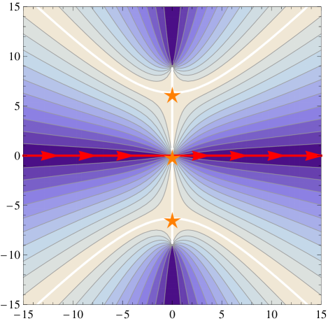
(a)

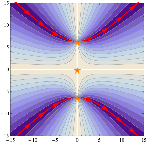
(b)

Figure 10: Phase contours of $k\left(f\left(z_{n}\right)-f_{n}\right)$. The orange stars are the saddles $z_{n}$, numbered from bottom to top. The red lines depict the steepest descent paths through $z_{n}$, where $k\left(f\left(z_{n}\right)-f_{n}\right)$ is real and positive. The colored contours map the absolute value of the argument of this quantity. Left panel: The steepest descent path through $z_{2}$, with $\theta_{k}=0$. Right panel: The paths through $z_{1,3}$ with $\theta_{k}=\pm\pi.$ All contours point from left to right. Saddle $2$ is adjacent to both $1$ and $3$, which are not mutually adjacent.

We shall now follow the formalism of Berry and Howls (1991) to compute the hyperasymptotic expansion. With $\theta_{k}\equiv\arg k$, we define our desired contour $C_{2}\left(\theta_{k}=0\right)$ as running on the real axis from left to right. In order to calculate the asymptotic series $T_{r}^{\left(2\right)}$ about $z_{2}$ (i.e., (Berry and Howls, 1991, Eq. (8))), we must define the root $\left[k\left(f\left(z\right)-f_{2}\right)\right]^{\frac{1}{2}}=\left[kz^{2}\left(\frac{1}{2}+gz^{2}\right)\right]^{\frac{1}{2}}$ so that it has phase $0$ on the outgoing edge and $\pi$ on the incoming edge of $C_{2}\left(\theta_{k}\right)$. We thus define

$$\forall z\in C_{2}:\qquad\left[k\left(f\left(z\right)-f_{2}\right)\right]^{\frac{1}{2}}\equiv k^{\frac{1}{2}}z\sqrt{\frac{1}{2}+gz^{2}}\,,$$ (126)

where $k^{\frac{1}{2}}$ is taken on the smooth manifold of the square root (i.e., it is continuous in $k$ and experiences no branch cuts, and thus is multi-valued), while $\sqrt{\frac{1}{2}+gz^{2}}$ is taken with respect to the principal branch of the square root, with a cut along the negative real axis. As such, as a function of $z$, the expression above is analytic on $C_{2}$, and specifically, only has branch cuts stemming from $\sqrt{2}z_{1}$ and $\sqrt{2}z_{3}$ along the imaginary line, both pointing away from $z_{2}$.

The asymptotic expansion around $z_{2}$ is then

$$T_{r}^{\left(2\right)} =\frac{\left(r-\frac{1}{2}\right)!}{2\pi i}\oint_{z_{2}}\frac{\left[\left(f\left(z\right)-f_{2}\right)\right]^{\frac{1}{2}}dz}{\left[f\left(z\right)-f_{2}\right]^{r+1}}$$

$$=\frac{\left(r-\frac{1}{2}\right)!}{2\pi i}\oint_{0}\frac{z\sqrt{\frac{1}{2}+gz^{2}}dz}{\left[z^{2}\left(\frac{1}{2}+gz^{2}\right)\right]^{r+1}}$$

$$=\frac{\left(r-\frac{1}{2}\right)!}{2\pi i}2^{\frac{1}{2}+r}\oint_{0}\sum_{t=0}^{\infty}\binom{-\frac{1}{2}-r}{t}\left(2g\right)^{t}z^{-1+2t-2r}dz$$

$$=\sqrt{2}\left(-4g\right)^{r}\frac{\Gamma\left(2r+\frac{1}{2}\right)}{r!}\,.$$ (127)

As expected, $T_{r}^{\left(2\right)}$ reproduces the asymptotic expansion obtained by a direct calculation in Subsection B.B.1thesubsection.

The first hyperseries iteration looks at the remainder of the sum $T^{\left(2\right)}\left(k\right)=\sum_{r}k^{-r}T_{r}^{\left(2\right)}$. This requires the adjacency topology of the saddles, that is, the saddle parings $n,\,m$ for which exists some $k$ that rotates $n$’s steepest-descent path so it reaches $m$. Since $2$’s steepest-descent path splits the complex plane into its top and bottom halves, no such path can exist between saddles $1$ and $3$, so they are not adjacent. However, $2$ is adjacent to both. It is easily verified that for $k=-1$ (or in general, $k$ with argument $\pm\pi$), the path $z_{2}\left(u\right)$ in (LABEL:hyperasymptotic_contours) coincides partially with $z_{1,3}\left(u^{\prime}\right)$ for some real $u^{\prime}<u$ (i.e. $z_{2}\left(u\right)$ “arrives late” at the contours $C_{1,3}\left(\theta_{k}=\pm\pi\right)$). For these arguments of $k$, the path $C_{1}$ has endpoints at $\left(\infty e^{-\frac{i\pi}{4}},\infty e^{-\frac{3i\pi}{4}}\right)$ and $C_{3}$ has endpoints $\left(\infty e^{+\frac{i\pi}{4}},\infty e^{+\frac{3i\pi}{4}}\right)$. Care must be taken when defining the direction of the contours: $C_{2}$ coincides with $C_{1}$ if we rotate it clockwise, so $k$ has to rotate in the other direction, meaning we encounter $C_{1}\left(\theta_{k}=+\pi\right)$, which points from left to right. Due to a similar argument, we encounter $C_{3}\left(\theta_{k}=-\pi\right)$, also pointing from left to right, which is obtained by rotating $C_{2}$ counterclockwise. In order to be consistent with the definition of $\arg k=-\arg F_{nm}$, we identify

$$\arg F_{21}=-\pi,\qquad\arg F_{23}=+\pi$$ (128)

despite the fact that they are numerically equal. The next step, performed in (Berry and Howls, 1991, Eq. (15)), sees us deforming the integration contour $\Gamma_{2}\left(\theta_{k}=0\right)$, a narrow strip that encircles $C_{2}\left(\theta_{k}=0\right)$ counterclockwise, into the sum of the contours $C_{1,3}$. The orientation anomalies $\gamma_{nm}$ are defined as $1$ if the deformation of $\Gamma_{n}$ requires reversing the direction of $C_{m}$, and $0$ otherwise. Both $C_{1,3}$ run from left to right, implying that $C_{1}$ encircles $C_{2}\left(0\right)=\mathbb{R}$ counterclockwise but $C_{3}$ does not, so $\gamma_{21}=0$ and $\gamma_{23}=1$.

The variable transformation (Berry and Howls, 1991, Eq. (16)) $u=v\left(f\left(z\right)-f_{2}\right)/F_{2m}$ does not yet uniquely define the inverse transformation of $\left[f\left(z\right)-f_{2}\right]^{\frac{1}{2}}$. Using our definition (126), one observes that the following holds:

$$\forall z\in C_{1}\left(+\pi\right):\qquad\arg\left\{z\sqrt{\frac{1}{2}+gz^{2}}\right\}=-\frac{\pi}{2}\ ,$$ (129)

$$\forall z\in C_{3}\left(-\pi\right):\qquad\arg\left\{z\sqrt{\frac{1}{2}+gz^{2}}\right\}=+\frac{\pi}{2}\ .$$ (130)

Thus, since $F_{23}$ and $F_{21}$ have opposite arguments, one has on $C_{3}\left(-\pi\right)$ that $\left[f\left(z\right)-f_{2}\right]^{\frac{1}{2}}=i\sqrt{\frac{u}{v}\left|F_{23}\right|}=+\sqrt{\frac{u}{v}}\times\sqrt{F_{23}}$, while on $C_{1}\left(\pi\right)$ one obtains $\left[f\left(z\right)-f_{2}\right]^{\frac{1}{2}}=-i\sqrt{\frac{u}{v}\left|F_{21}\right|}=+\sqrt{\frac{u}{v}}\times\sqrt{F_{21}}$. Indeed, no additional sign adjustments are necessary.

Next, we require the coefficients $T_{r}^{\left(1,3\right)}$. For this we now define

$$\forall z\in C_{1}\left(\pi\right)\cup C_{3}\left(-\pi\right):\,\left[f\left(z\right)-f_{1,3}\right]^{\frac{1}{2}}\equiv\sqrt{g}\left(z-z_{1}\right)\left(z-z_{3}\right)\ .$$ (131)

This can be verified to give the correct phases: On the outgoing edge of $C_{1}$, $\arg\,z\sim-\frac{\pi}{4}$, so $k^{\frac{1}{2}}z^{2}$, with $\arg\,k=\pi$ has phase 0. On the outgoing edge of $C_{3}$, $\arg\,z\sim\frac{\pi}{4}$ and $\arg k=-\pi$, and again the required condition holds. The coefficients at $z_{1}$ are then

$$T_{r}^{\left(1\right)} =\frac{\left(r-\frac{1}{2}\right)!}{2\pi i}\oint_{z_{1}}\frac{\left[\left(f\left(z\right)-f_{1}\right)\right]^{\frac{1}{2}}dz}{\left[f\left(z\right)-f\left(z_{1}\right)\right]^{r+1}}$$

$$=\frac{\left(r-\frac{1}{2}\right)!}{2\pi i}\oint_{z_{1}}\frac{\sqrt{g}\left(z-z_{1}\right)\left(z-z_{3}\right)dz}{\left[g\left(z-z_{1}\right)^{2}\left(z-z_{3}\right)^{2}\right]^{r+1}}$$

$$=\frac{\left(r-\frac{1}{2}\right)!}{2\pi i}g^{-r-\frac{1}{2}}\oint_{0}z{}^{-2r-1}\left(z+z_{1}-z_{3}\right)^{-2r-1}dz$$

$$=\frac{\left(r-\frac{1}{2}\right)!}{2\pi i}g^{-r-\frac{1}{2}}\oint_{0}\sum_{t=0}^{\infty}\binom{-2r-1}{t}z{}^{t-2r-1}\left(z_{1}-z_{3}\right)^{-t-2r-1}dz$$

$$=g^{-r-\frac{1}{2}}\left(z_{1}-z_{3}\right)^{-4r-1}\frac{\Gamma\left(2r+\frac{1}{2}\right)4^{r}}{r!}\,.$$ (132)

Clearly, for $T^{\left(3\right)}$, the roles of $z_{1}$ and $z_{3}$ are reversed, so we gain a $\left(-1\right)^{4r+1}=-1$ relative sign. $z_{1}-z_{3}=-\frac{i}{\sqrt{g}}$, so we finally obtain

$$T_{r}^{\left(1\right)}=-T_{r}^{\left(3\right)}=i\frac{\left(4g\right)^{r}\Gamma\left(2r+\frac{1}{2}\right)}{r!}\,.$$ (133)

Resurgence is now readily apparent: Up to prefactors, $T_{r}^{\left(1,3\right)}$ are the alternating version of $T_{r}^{\left(2\right)}$.

Lastly, for the post-leading hyper-iteration, we need to examine the modified integrals $\int_{C_{1,3}\left(\pm\pi\right)}e^{-f\left(z\right)}dz$. The saddles $z_{1}$ and $z_{3}$ are not adjacent to each other: The contour $C_{3}\left(\theta_{k}\right)$ never leaves the top half of the complex plane, except for $\arg\,k$ which is a multiple of $2\pi$, when it coincides with half of the real line. The same applies to $C_{1}$ in the lower half. Thus, they could only meet on the real line, but this just means that both of them coincide with $C_{2}\left(0\right)$. This implies that we would deform $\Gamma_{1,3}$ in both cases to the real line. With both cases $C_{2}$ is obtained by “rotating” $C_{1,3}$ back, so both encounter $C_{2}\left(\theta_{k}=0\right)$. Thus, now the two singulants have the same phase, $\arg F_{12}=\arg F_{32}=0$. We observe that

$$\forall z\in C_{2}\left(0\right):\qquad\arg\left\{\sqrt{g}\left(z-z_{1}\right)\left(z-z_{3}\right)\right\}=0\,,$$ (134)

as the expression in the parenthesis is $z^{2}+\frac{1}{4g}$, which is real and positive, and no manual sign corrections are necessary, as $\left[f\left(z\right)-f_{m}\right]^{\frac{1}{2}}=+\sqrt{\frac{u}{v}}\times\sqrt{F_{m2}}$ for $m=1$ and $3$. However, during the deformation of $\Gamma_{1}$ into $C_{2}\left(0\right)$, we had to reverse the direction of $\Gamma_{1}$ ($C_{2}\left(0\right)$ encircles $C_{1}\left(\pi\right)$ clockwise). Thus, we again have an orientation anomaly of $\gamma_{12}=1$. To summarize,

$$\gamma_{23}=\gamma_{12}=1,\qquad\gamma_{21}=\gamma_{32}=0\,.$$ (135)

The hyperasymptotic trans-series is composed of several hyperseries, or iterations. Each iteration is the asymptotic expansion of the previous iteration’s remainder, performed around the saddles adjacent to the saddle about which the previous hyperseries was expanded. This successive expansion around adjacent saddles is a called a “scattering path,” and the trans-series is the summation over all such paths.

Each hyperseries is terminated earlier than the preceding one, so the scheme naturally halts after a finite number of terms. We choose to demonstrate the expansion for $g=\frac{1}{160}$. (Berry and Howls, 1991, Eq. (30)) allows us to determine the truncation of each hyperseries: Saddles $1$ and $3$ are not adjacent to each other, all the scattering paths consist of scattering back and forth from saddle $2$. Since the singulants $\left|F_{12}\right|=\left|F_{32}\right|=\frac{1}{16g}$ are of equal magnitude, all paths with the same number of scatterings will terminate at the same order, and at every level the order is halved. We have

$$N\left(2\right)=\frac{1}{16g}=10,\quad N\left(21\right)=N\left(23\right)=5,\quad N\left(212\right)=N\left(232\right)=2,$$

$$N\left(2121\right)=N\left(2123\right)=N\left(2321\right)=N\left(2323\right)=1\,.$$ (136)

where $N\left(nm\ldots\right)$ is the truncation of the scattering path that originates at $z_{n}$, scatters to $z_{m}$, and so on.

Additionally, we note an emerging pattern: (i) For an odd number of scatterings from saddle $z_{2}$, the scattering chain ends at either $z_{1}$ or $z_{3}$. At $z_{3}$ we incur a minus sign due to traversing $\gamma_{23}$, but as $T_{r}^{\left(1\right)}=-T_{r}^{\left(3\right)}$, these two paths add constructively. (ii) For an even number of scatterings, the chain ends at $z_{2}$. No matter the path, each edge has been traversed the same number of times back and forth, so all paths have gained the same amount of minus signs. Ergo, paths related by exchanges $1\leftrightarrow 3$ again add constructively.

This suggests that one can only sum over the length of scattering paths, assuming only saddle $z_{3}$ or $z_{1}$ exists, and multiply by the symmetry factor $2^{\text{number of scatterings to $z_{3}$}}$.

The last ingredients we require are the terminants $K_{r}$. The first-level terminants can be expressed as (Berry and Howls, 1990, Appendix B)

$$K_{r}^{\left(01\right)} =\frac{\left(-1\right)^{\gamma_{01}}}{2\pi iF_{01}^{N_{0}-r}}\int_{0}^{\infty}dv_{0}\frac{v_{0}^{N_{0}-r-1}e^{-v_{0}}}{1-v_{0}/F_{01}}$$

$$=\frac{\left(-1\right)^{\gamma_{01}+r+N_{0}}}{2\pi i}e^{-F_{01}}\Gamma\left(N_{0}-r\right)\Gamma\left(1+r-N_{0},-F_{01}\right)$$

$$=\frac{\left(-1\right)^{\gamma_{01}}}{2\pi i}\left(-e^{-F_{01}}\text{E}_{1}(-F_{01})-\sum_{m=0}^{N_{0}-r-2}\frac{m!}{F_{01}^{m+1}}\right)\,,$$ (137)

with the indices $01$ representing the starting saddle of the path and the first scattering, so $0\,=\text{saddle 2}$ and $1\,=\text{either $1$ or 3}$. The next terminant $K^{\left(012\right)}$ is found by numerical integration, while the last required terminant, $K^{\left(0123\right)}$ is approximated by the same method as in Ref. Berry and Howls (1990). We thus obtain

$$\mathcal{Z}_{HA} =\sum_{r=0}^{N\left(2\right)}T_{r}^{\left(2\right)}+2\sum_{r=0}^{N\left(23\right)}K^{\left(23\right)}T_{r}^{\left(3\right)}+2\sum_{r=0}^{N\left(232\right)}K^{\left(232\right)}T_{r}^{\left(2\right)}+4\sum_{r=0}^{N\left(2323\right)}K^{\left(2323\right)}T_{r}^{\left(3\right)}\,.$$ (138)

The relative size of each term in this expansion is depicted in 11.

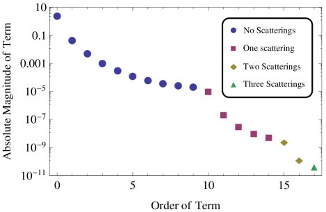
Figure 11: Plotted are the absolute values of the successive terms in the hyperasymptotic approximation of $\mathcal{Z}$, after multiplication by their symmetry factors as in (138), for $g=\frac{1}{160}$. For this value, the hyperseries naturally halts after three scatterings. The zeroth and first levels are calculated exactly, the second level by numerical integration, and the last stage is approximated. The final relative error of the trans-series after it is summed is $5.7\times 10^{-12}$.

For $g=\frac{1}{160}$, the ultimate relative error achieved by this approximation is about $5.7\times 10^{-12}$. This may be compared with the error predicted by (Berry and Howls, 1991, Eqs. (32) and (34))

$$R_{HA}\left(S\right)=\frac{e^{-F}}{\sqrt{2\pi F}}\times\prod_{s=1}^{S}\frac{2^{\frac{s}{2}}}{\sqrt{\pi F}}e^{-\frac{\ln 2}{2^{s-2}}F}\times 2^{\left\lfloor\frac{S+1}{2}\right\rfloor}\,,$$ (139)

where $F=\left|F_{21}\right|=\frac{1}{16g}$, $S$ the number of scattering stages, and $k=1$ is assumed. The three factors correspond to the remainder after the zeroth stage, the successive improvements of each hyperseries level, and the number of (numerically identical) paths at the last stage, whose remainders we expect will add constructively. $S$ of course is determined by $g$ (roughly $\log_{2}\frac{1}{16g}$, as we saw above). Setting $g=\frac{1}{160}$ and $S=3$ (and dividing by the exact $\mathcal{Z}\left(g\right)$), we obtain an expected relative error of $4.0\cdot 10^{-12}$, in close agreement with our numerical result.

It is worth noting that for $g$ much smaller than $\frac{1}{160}$, evaluation of the complete hyperseries becomes impractical: The approximation used to determine $K^{\left(0123\right)}$ (and all subsequent terminants) only gives about 3 correct significant digits of the terminant; thus, only a couple of additional decimal places of the final result may be extracted from the third and subsequent stages before this approximation “washes out” the true value of $\mathcal{Z}$.

The hyperasymptotic treatment of the Airy function is simpler since it only has two saddles. The exponential function over which we integrate is $f\left(t\right)=\sqrt{z}t^{2}-\frac{i}{3}t^{3}$ [per the integral representation (83)], which has two saddles, at $t_{1}=0$ and $t_{2}=-2i\sqrt{z}$, and the singulants are $F_{21}=-F_{12}=\frac{4}{3}z^{\frac{3}{2}}$. The first saddle is the starting point for the hyperasymptotic scattering paths, and the expansion coefficients $T_{r}^{(1)}$ are those given in (LABEL:Airy_tilde_standard_asymptotic_form). It can be shown that at the other saddle, $T_{r}^{(2)}=i(-1)^{r}T_{r}^{(1)}$ and that $\gamma_{12}=0$ and $\gamma_{21}=1$. The terminants are calculated in the same manner as before.

Furthermore, in their introductory paper to hyperasymptotics Berry and Howls (1990), Berry and Howls specifically analyze the Airy function and give an error estimate (Berry and Howls, 1990, Eq. (35)) ,

$$R_{Hyp}^{\left(N\right)}=\sqrt{\frac{2}{\pi}}\left|F\right|^{\frac{1}{4}\log_{2}\left|F\right|+\frac{3}{4}-\log_{2}\left(3\sqrt{2\pi}\right)}e^{-\left(1+2\ln 2\right)\left|F\right|}\,,$$ (140)

with $F=\frac{4}{3}z^{\frac{3}{2}}$ the singulant.

B.3 Chebyshev Polynomial Approximation by Lanczos’s $\tau$ Method

With the definition (LABEL:Z_definition), we have

$$\frac{d\mathcal{Z}}{dg}=-\int_{-\infty}^{\infty}x^{4}e^{-\left[\frac{1}{2}x^{2}+gx^{4}\right]}dx\,.$$ (141)

However, performing the rescaling $y=g^{\frac{1}{4}}x$, we have

$$\mathcal{Z}\left(g\right)g^{\frac{1}{4}}=\int_{-\infty}^{\infty}e^{-\left[\frac{1}{2}g^{-\frac{1}{2}}y^{2}+y^{4}\right]}dy\,,$$ (142)

so we can differentiate w.r.t $w=\sqrt{g}$, obtaining

$$w^{\frac{5}{2}}\frac{d\mathcal{Z}}{dw}+\frac{1}{2}w^{\frac{3}{2}}\mathcal{Z}=\int_{-\infty}^{\infty}\frac{y^{2}}{2}e^{-\left[\frac{1}{2}w^{-1}y^{2}+y^{4}\right]}dy\,,$$

$$w^{\frac{5}{2}}\frac{d^{2}\mathcal{Z}}{dw^{2}}+3w^{\frac{3}{2}}\frac{d\mathcal{Z}}{dw}+\frac{3}{4}w^{\frac{1}{2}}\mathcal{Z}=\int_{-\infty}^{\infty}\frac{y^{4}}{4w^{2}}e^{-\left[\frac{1}{2}w^{-1}y^{2}+y^{4}\right]}dy\,,$$

$$w^{2}\frac{d^{2}\mathcal{Z}}{dw^{2}}+3w\frac{d\mathcal{Z}}{dw}+\frac{3}{4}\mathcal{Z}=-\frac{1}{4}\frac{d\mathcal{Z}}{dg}=-\frac{1}{4}\frac{d\mathcal{Z}}{dw}\frac{1}{2w}\,\,.$$ (143)

One may repose this equation in terms of $\mathcal{Z}\left(g\right)$, which yields

$$16g^{2}\mathcal{Z}^{\prime\prime}\left(g\right)+\left(1+32g\right)\mathcal{Z}^{\prime}\left(g\right)+3\mathcal{Z}\left(g\right)=0\,.$$ (144)

With an ODE for $\mathcal{Z}\left(g\right)$ in hand, we would like to integrate this equation from $g=0$, subject to the boundary condition $\mathcal{Z}\left(0\right)=\sqrt{2\pi}$. Note that $g=0$ is a singular point of (LABEL:Anharmonic_Z4_ODE), so we do not necessarily require a second boundary condition.

Next, we outline the procedure of the $\tau$ method, due to Lanczos Boyd (1999, 2001): To obtain the $N$-th order approximation of $\mathcal{Z}$, instead of solving (LABEL:Anharmonic_Z4_ODE) approximately, we will obtain an exact solution to an approximate equation,

$$16g^{2}\mathcal{Z}^{\prime\prime}\left(g\right)+\left(1+32g\right)\mathcal{Z}^{\prime}\left(g\right)+3\mathcal{Z}\left(g\right)=\tau T_{N}^{*}\left(\frac{g}{s}\right)\,,$$ (145)

with $T_{N}^{*}\left(\frac{g}{s}\right)=T_{N}\left(2\frac{g}{s}-1\right)$ the shifted Chebyshev polynomials of order $N$; $s\geq g$ a parameter that stretches the polynomials, which are normally defined on the interval $\left[0,1\right]$; and $\tau$ a new variable which we need to solve for.

This equation may be solved by a power series in $g$. Crucially, introducing $\tau$ permits a solution which terminates after a finite power $g^{N}$. Denoting the coefficients of the power series by $\left\{a_{n}\right\}_{n=0}^{N}$, we have $N+2$ unknowns (including $\tau$), and $N+1$ equations obtained by equating the coefficients of $\left\{g^{n}\right\}_{n=0}^{N}$ on both sides of (LABEL:Anharmonic_Z4_Lanczos_Equation). Together with the boundary condition $a_{0}=\mathcal{Z}\left(0\right)=\sqrt{2\pi}$, we have a system of $N+2$ linear equations. The resulting coefficients $\left\{a_{n}\right\}$ are $s$-dependent, and thus we finish the procedure by choosing $s=g$ so that the entire domain of $T_{N}^{*}$ is utilized without any “waste.” The resulting solution for $\mathcal{Z}\left(g\right)$ is now a rational function of $g$. This $\tau$ approximation can be computed systematically with ease by any computer algebra software.

In the case of the Airy function, we note that $\mathrm{Ai}\left(z\right)$ satisfies the second-order differential equation (Abramowitz and Stegun, 1964, Eq. (10.4.1))

$$\frac{d^{2}\mathrm{Ai}\left(z\right)}{dz^{2}}=z\cdot\mathrm{Ai}\left(z\right)\,.$$ (146)

Defining $\tilde{\mathrm{Ai}}\left(z\right)=2\pi z^{\frac{1}{4}}e^{\frac{2}{3}z^{\frac{3}{2}}}\mathrm{Ai}\left(z\right)$ as before, and changing variables by defining $f\left(x\right)=\tilde{\mathrm{Ai}}\left(x^{-\frac{2}{3}}\right)$ (so again $x=z^{-\frac{3}{2}}$), one obtains a new differential equation,

$$5f\left(x\right)+24\left(2+3x\right)f^{\prime}\left(x\right)+36x^{2}f^{\prime\prime}\left(x\right)=0\,.$$ (147)

With the boundary condition $f\left(0\right)=\tilde{\mathrm{Ai}}\left(z\rightarrow\infty\right)=\sqrt{\pi}$, we may apply the $\tau$ method again, and $\mathrm{Ai}\left(z\right)$ is then recovered by the appropriate substitutions.

B.4 Padé Approximants

With the usual perturbative expansion of $\mathcal{Z}$ in Subsection B.B.1thesubsection, we define the Padé approximation of $\mathcal{Z}$ of order $N$ to be Bender and Orszag (1978)

$$\mathcal{Z}_{\text{Pad\'{e}}}^{\text{$\left(N\right)$}}\left(g\right)=\frac{P\left(g\right)}{Q\left(g\right)}\,,$$ (148)

with $P\left(x\right)$ and $Q\left(x\right)$ polynomials of order $\frac{N}{2}$ in $g$, such that the expansion of $P/Q$ in powers of $g$ reproduces the first $N+1$ terms of (LABEL:Z4_Superasymptotic_Series) (neglecting the truncation at $N_{0})$. Note that his method can only be evaluated at even orders: Each polynomial has $\frac{N}{2}+1$ degrees of freedom, while a total rescaling of both by the same constant does not change the approximation, so we lose a single degree of freedom and are left with $N+1$ degrees, corresponding to the $N+1$ terms of the $N^{\text{th}}$-order asymptotic series. We obtain this approximation by using Mathematica’s PadeApproximant routine Wolfram Research, Inc. .

This method can be applied just as easily to the perturbative power expansion of $\mathrm{Ai}\left(z\right)$ in (LABEL:Airy_tilde_standard_asymptotic_form).

References

- Boyd (1999) J. P. Boyd, Acta Applicandae Mathematica 56, 1 (1999).
- Feynman (1949) R. P. Feynman, Phys. Rev. 76, 769 (1949).
- Zinn-Justin (2002) J. Zinn-Justin, Quantum Field Theory and Critical Phenomena, 4th ed. (Clarendon Press, Oxford, 2002).
- Costin (2008) O. Costin, Asymptotics and Borel Summability (CRC press, New York, 2008).
- Berry and Howls (1990) M. V. Berry and C. J. Howls, Proc. R. Soc. A 430, 653 (1990).
- Cherman et al. (2015) A. Cherman, D. Dorigoni, and M. Ünsal, J. High Energy Phys. 10, 56 (2015).
- Aniceto et al. (2018) I. Aniceto, G. Başar, and R. Schiappa, preprint arXiv:1802.10441 (2018).
- Bender and Orszag (1978) C. M. Bender and S. A. Orszag, Advanced Mathematical Methods for Scientists and Engineers (McGraw-Hill, New York, 1978).
- (9) N. H. Abel, letter to Holmboe, January 18, 1826.
- Peskin and Schroder (1995) M. E. Peskin and D. V. Schroder, An Introduction to Quantum Field Theory (Perseus Books, Reading, MA, 1995).
- Strogatz (1994) S. H. Strogatz, Nonlinear Dynamics and Chaos (Perseus Books, Reading, MA, 1994).
- Schwartz and Katzav (2008) M. Schwartz and E. Katzav, J. Stat. Mech: Theory Exp. 2008, P04023 (2008).
- Cohen et al. (2016) A. Cohen, S. Bialy, and M. Schwartz, Physica A 463, 503 (2016).
- Schwartz and Edwards (1992) M. Schwartz and S. F. Edwards, Europhys. Lett. 20, 301 (1992).
- Schwartz and Edwards (1998) M. Schwartz and S. F. Edwards, Phys. Rev. E 57, 5730 (1998).
- Kardar et al. (1986) M. Kardar, G. Parisi, and Y.-C. Zhang, Phys. Rev. Lett. 56, 889 (1986).
- Wiese (1998) K. J. Wiese, J. Stat. Phys. 93, 143 (1998).
- Katzav and Schwartz (1999) E. Katzav and M. Schwartz, Phys. Rev. E 60, 5677 (1999).
- Schwartz and Edwards (2002) M. Schwartz and S. F. Edwards, Physica A 312, 363 (2002).
- Katzav (2003) E. Katzav, Phys. Rev. E 68, 046113 (2003).
- Katzav and Schwartz (2004a) E. Katzav and M. Schwartz, Phys. Rev. E 69, 052603 (2004a).
- Katzav and Schwartz (2004b) E. Katzav and M. Schwartz, Phys. Rev. E 70, 011601 (2004b).
- Katzav and Adda-Bedia (2006) E. Katzav and M. Adda-Bedia, Europhys. Lett. 76, 450 (2006).
- Katzav et al. (2007) E. Katzav, M. Adda-Bedia, M. Ben Amar, and A. Boudaoud, Phys. Rev. E 76, 051601 (2007).
- Edwards and Schwartz (2002) S. F. Edwards and M. Schwartz, Physica A 303, 357 (2002).
- Li et al. (1996) M. S. Li, T. Nattermann, H. Rieger, and M. Schwartz, Phys. Rev. B 54, 16024 (1996).
- Negele and Orland (1998) J. W. Negele and H. Orland, Quantum Many-Particle Systems (Perseus Books, Reading, MA, 1998).
- Yukalov (1976) V. I. Yukalov, Moscow Univ. Phys. Bull. 31, 10 (1976).
- Yukalov and Yukalova (1999) V. I. Yukalov and E. P. Yukalova, Ann. Phys. 277, 219 (1999).
- Zinn-Justin and Seznec (1979) J. Zinn-Justin and R. Seznec, J. Math. Phys. 20, 1398 (1979).
- Zinn-Justin (2010) J. Zinn-Justin, Appl. Numer. Math. 60, 1454 (2010).
- Stevenson (1981) P. M. Stevenson, Phys. Rev. D 23, 2916 (1981).
- Jones (1990) H. F. Jones, Nucl. Phys. B Proc. Suppl. 16, 592 (1990).
- Mattingly and Stevenson (1994) A. C. Mattingly and P. M. Stevenson, Phys. Rev. D 49, 437 (1994).
- Stevenson (2013) P. M. Stevenson, Nucl. Phys. B 868, 38 (2013).
- Abdalla et al. (2009) M. C. B. Abdalla, J. A. Helayël-Neto, D. L. Nedel, and C. R. Senise, Physical Review D 80, 065002 (2009).
- Kneur et al. (2007) J.-L. Kneur, M. B. Pinto, R. O. Ramos, and E. Staudt, Phys. Rev. D 76, 045020 (2007).
- Kneur et al. (2010) J.-L. Kneur, M. B. Pinto, and R. O. Ramos, Phys. Rev. C 81, 065205 (2010).
- Braaten and Radescu (2002) E. Braaten and E. Radescu, Phys. Rev. Lett. 89, 271602 (2002).
- Yukalov (1985) V. I. Yukalov, Phys. Rev. B 32, 436 (1985).
- Yamada (2007) H. Yamada, Phys. Rev. D 76, 045007 (2007).
- Kneur et al. (2003) J.-L. Kneur, M. B. Pinto, and R. O. Ramos, Phys. Rev. A 68, 043615 (2003).
- de Souza Cruz et al. (2001) F. F. de Souza Cruz, M. B. Pinto, and R. O. Ramos, Phys. Rev. B 64, 014515 (2001).
- Buckley et al. (1993) I. R. C. Buckley, A. Duncan, and H. F. Jones, Phys. Rev. D 47, 2554 (1993).
- Guida et al. (1995) R. Guida, K. Konishi, and H. Suzuki, Ann. Phys. 241, 152 (1995).
- Guida et al. (1996) R. Guida, K. Konishi, and H. Suzuki, Ann. Phys. 249, 109 (1996).
- Abramowitz and Stegun (1964) M. Abramowitz and I. A. Stegun, Handbook of Mathematical Functions, Vol. 55 (Dover, New York, 1964).
- Pernice and Oleaga (1998) S. A. Pernice and G. Oleaga, Phys. Rev. D 57, 1144 (1998).
- Dyson (1952) F. J. Dyson, Phys. Rev. 85, 631 (1952).
- Bender and Wu (1969) C. M. Bender and T. T. Wu, Phys. Rev. 184, 1231 (1969).
- Bender and Wu (1973) C. M. Bender and T. T. Wu, Phys. Rev. D 7, 1620 (1973).
- (52) DLMF, “NIST Digital Library of Mathematical Functions,” http://dlmf.nist.gov/.
- (53) Wolfram Research, Inc., “Mathematica, Version 11.2,” Champaign, IL, 2017.
- Berry and Howls (1991) M. V. Berry and C. J. Howls, Proc. R. Soc. A 434, 657 (1991).
- Boyd (2001) J. P. Boyd, Chebyshev and Fourier Spectral Methods (Dover, New York, 2001).
- Vallée and Soares (2010) O. Vallée and M. Soares, Airy Functions and Applications to Physics (Imperial College Press, London, 2010).
- Stokes (1864) G. G. Stokes, Trans. Camb. Phil. Soc. 10, 105 (1864).
- Blencowe et al. (1998) M. P. Blencowe, H. F. Jones, and A. P. Korte, Phys. Rev. D 57, 5092 (1998).
- Berry (1989a) M. V. Berry, Proc. R. Soc. A 422, 7 (1989a).
- Berry (1989b) M. V. Berry, Publications Mathématiques de l’IHÉS 68, 211 (1989b).
- Olver (1990) F. W. J. Olver, in Asymptotic and Computational Analysis, Vol. 124, edited by R. Wong (Marcel Dekker, 1990) p. 329.
- Rosa et al. (2016) D. S. Rosa, R. L. S. Farias, and R. O. Ramos, Physica A 464, 11 (2016).
- Bender et al. (1994) C. M. Bender, A. Duncan, and H. F. Jones, Phys. Rev. D 49, 4219 (1994).
- Arvanitis et al. (1995) C. Arvanitis, H. F. Jones, and C. S. Parker, Phys. Rev. D 52, 3704 (1995).
- Turbiner (1984) A. V. Turbiner, Usp. Fiz. Nauk 144, 35 (1984).
- Turbiner (2005) A. V. Turbiner, Lett. Math. Phys. 74, 169 (2005).
- Serone et al. (2017a) M. Serone, G. Spada, and G. Villadoro, J. High Energy Phys. 05, 56 (2017a).
- Serone et al. (2017b) M. Serone, G. Spada, and G. Villadoro, Phys. Rev. D 96, 021701 (2017b).