Constrained Deep Learning using Conditional Gradient and Applications in Computer Vision

Abstract

A number of results have recently demonstrated the benefits of incorporating various constraints when training deep architectures in vision and machine learning. The advantages range from guarantees for statistical generalization to better accuracy to compression. But support for general constraints within widely used libraries remains scarce and their broader deployment within many applications that can benefit from them remains under-explored. Part of the reason is that Stochastic gradient descent (SGD), the workhorse for training deep neural networks, does not natively deal with constraints with global scope very well. In this paper, we revisit a classical first order scheme from numerical optimization, Conditional Gradients (CG), that has, thus far had limited applicability in training deep models. We show via rigorous analysis how various constraints can be naturally handled by modifications of this algorithm. We provide convergence guarantees and show a suite of immediate benefits that are possible — from training ResNets with fewer layers but better accuracy simply by substituting in our version of CG to faster training of GANs with 50% fewer epochs in image inpainting applications to provably better generalization guarantees using efficiently implementable forms of recently proposed regularizers.

Keywords: Constrained Deep Learning, Conditional Gradient Algorithms, Path Norm

1 Introduction

The learning or fitting problem in deep neural networks in the supervised setting is often expressed as the following stochastic optimization problem,

$$\min_{W}\mathop{\mathbb{E}}\limits_{(x,y)\sim\mathcal{D}}\mathcal{L}(W;(x,y))$$ (1)

where $W=W_{1}\times\cdots\times W_{l}$ denotes the Cartesian product of the weight matrices of the network with $l$ layers that we seek to learn from the data $(x,y)$ sampled from the underlying distribution $\mathcal{D}$. Here, $x$ can be thought of the “features” (or predictor variables) of the data and $y$ denotes the “labels” (or the response variable). The variable $W$ parameterizes the function that we desire to learn that predicts the labels given the features whose accuracy is measured using the loss function $\mathcal{L}$. In the unsupervised setting, we do not have a notion of labels, hence the common practice is to inject some prior knowledge or inductive bias into the loss $\mathcal{L}$. For simplicity, the specification above is intentionally transparent to the activation function we use between the layers and the specific network architecture. Most common instantiations of the above task are non-convex but results in the last five years demonstrate that reasonable minimizers that generalize well to test data can be found via SGD and its variants. Recent results have also explored the interplay between the overparameterization of the network, its degrees of freedom and issues related to global optimality Haeffele and Vidal (2015); Janzamin et al. (2015); Soudry and Carmon (2016).

Regularizers. Independent of the network architecture we choose to deploy for a given task, a practitioner may often want to impose additional constraints or regularizers, pertinent to the application domain of interest. In fact, the use of task specific constraints to improve the behavioral performance of neural networks, both from a computational and statistical perspective, has a long history dating back at least to the 1980s Platt and Barr (1988); Zhang and Constantinides (1992). These ideas are being revisited recently Rudd et al. (2014) motivated by generalization, convergence or simply as a strategy for compression Cheng et al. (2017); Han et al. (2015). However, using constraints on the types of architectures that are common in modern computer vision problems is still being actively researched by various groups. For example, Mikolov et al. (2014) demonstrated that training Recurrent Networks can be accelerated by constraining a part of the recurrent matrix to be close to identity. Sparsity and low-rank encouraging constraints have shown promise in a number of settings Tai et al. (2015); Liu et al. (2015). In an interesting paper, Pathak et al. (2015) showed that linear constraints on the output layer improves the accuracy on a semantic image segmentation task. Márquez-Neila et al. (2017) showed that hard constraints on the output layer yield competitive results on the 3D human pose estimation task and Oktay et al. (2017) used anatomical constraints for cardiac image analysis. The above discussion suggests that while there are some results demonstrating the value of specific constraints for specific problems, the development is still in a nascent stage. It is, therefore, not surprising that the existing software libraries and APIs for deep learning (DL) in vision and machine learning offer little to no support for constraints. For example, Keras only offers support for simple bound constraintsCharles (2013).

Optimization Schemes. Let us set aside the issue of constraints for a moment and discuss the choice of the optimization schemes that are in use today. There is little doubt that SGD algorithms dominate the landscape of DL problems in vision and machine learning. Instead of evaluating the loss and the gradient over the full training set, SGD simply computes the gradient of the parameters using a few training examples. It mitigates the cost of running back propagation over the full training data and comes with various theoretical guarantees as well Hardt et al. (2016); Raginsky et al. (2017). The reader will notice that part of the reason that constraints have not been intensively explored in a broader range of problems may have to do with the interplay between constraints and the SGD algorithm Márquez-Neila et al. (2017). While some regularizers and “local” constraints are easily handled within SGD, some others require a great deal of care and can adversely affect convergence and practical runtime Bengio (2012). There are also a broad range of constraints where SGD is unlikely to work well based on theoretical results known today — and it remains an open question in optimization Johnson and Zhang (2013); Defazio et al. (2014). We note that algorithms other than the standard SGD have remained a constant focus of research in the community since they offer many theoretical advantages that can also be easily translated to practice Dauphin et al. (2015); Grubb and Bagnell (2010). These include adaptive sub-gradient methods such as Adagrad Duchi et al. (2011), the RMSprop algorithm Dauphin et al. (2015) which addresses the issue of ill-conditioning in Deep Networks with a normalized form of SGD, and various adaptive schemes for learning rate adjustments Zeiler (2012) and utilizing the momentum method Kingma and Ba (2014). However, the reader will notice that these methods only impose constraints in a “local” fashion since the computational cost of imposing global constraints using SGD-based methods becomes extremely high Pathak et al. (2015). We explore this issue in depth in the next section.

2 Why do we need to impose constraints?

The question of why constraints are needed for statistical learning models in vision and machine learning can be equivalently restated in terms of the need for regularization in setting up learning models — a notion that is well known but will be precisely stated shortly. Recall that regularization schemes in one form or another go nearly as far back as the study of fitting models to observations of data Wahba (1990); Mundle (1959). Broadly speaking, such schemes can be divided into two related categories: algebraic and statistical (or probabilistic). The first category may refer to problems that are otherwise not possible or difficult to solve, also known as ill-posed problems Tikhonov et al. (1987). For example, without introducing some additional piece of information, it is not possible to solve a linear system of equations $Ax=b$ in which the number of observations (rows of $A$) is less than the number of degrees of freedom (columns of $A$). In the second category, one may use regularization as a way of “explaining” data using simple hypotheses rather than complex ones, for example, the minimum description length principle Rissanen (1985). The underlying rationale is that, complex hypotheses are less likely to be accurate on the unobserved samples (also known as Occam’s razor). In other words, the generalizability of models diminish as the complexity of the model increases for a fixed dataset size. Or equivalently, we need more data to train complex models. Recent developments on the theoretical side of DL showed that imposing simple but global constraints on the parameter space of deep networks is an effective way of analyzing the learning theoretic properties including sample complexity and generalization error Neyshabur et al. (2015b). Hence we seek to solve,

$$\min_{W}\mathop{\mathbb{E}}\limits_{(x,y)\sim\mathcal{D}}\mathcal{L}(W;(x,y))+\mu R(W)$$ (2)

where $R(\cdot)$ is a suitable regularization function for a fixed $\mu>0$. We usually assume that $R(\cdot)$ is simple, for example, in the sense that the gradient can be computed efficiently. Using the Lagrangian interpretation, Problem (2) is the same as the following constrained formulation,

$$\min_{W}\mathop{\mathbb{E}}\limits_{(x,y)\sim\mathcal{D}}\mathcal{L}(W;(x,y))~{}\text{s.t.}~{}R(W)\leq\lambda$$ (3)

where $\lambda>0$. Note that when the loss function $\mathcal{L}$ is convex, both the above problems are equivalent in the sense that given $\mu>0$ in (2), there exists a $\lambda>0$ in (3) such that the optimal solutions to both the problems coincide (see sec 1.2 in Bach et al. (2012)). In practice, both $\lambda$ and $\mu$ are chosen by standard statistical procedures such as cross validation.

Finding Pareto Optimal Solutions: On the other hand, when the loss function is nonconvex as is typically the case in DL, formulation (3) is more powerful than (2). Let us see why: for a fixed $\lambda>0$, there might be solutions $W^{*}_{\lambda}$ of (3) for which there exists no $\mu>0$ such that $W^{*}_{\lambda}=W^{*}_{\mu}$ whereas any solution of problem (2) can be obtained for some $\mu$ in (3), see section 4.7 in Boyd and Vandenberghe (2004). It turns out that it is easier to understand this phenomenon through the lens of multiobjective optimization. In multiobjective optimization, care has to be taken to even define the notion of optimality of feasible points (let alone computing them efficiently) depending on the problem. Among various notions of optimality, we will now argue that Pareto optimality is the most suited for our goal.

Recall that our goal is to find $W$’s that achieve low training error and are at the same time “simple” (as measured by $R$). In this context, a pareto optimal solution is a point $W$ such that none of $\mathcal{L}(W)$ or $R(W)$ in (3) or (2) can be made better without making the other worse, thus capturing the essence of overfitting effectively. In practice, there are many algorithms to find pareto optimal solutions and this is where problem (3) dominates (2). Specifically, formulation (2) falls under the category of “scalarization” technique whereas (3) is $\epsilon$-constrained technique. It is well known that when the problem is nonconvex, $\epsilon$-constrained technique yields pareto optimal solutions whereas scalarization technique does not!

Finally, we should note that even when the problems (2) and (3) are equivalent, in practice, algorithms that are used to solve them can be very different.
Our contributions: We show that many interesting global constraints of interest in vision/machine learning after reformulations can be enforced using a classical optimization technique that has not been deployed much at all in training deep learning models. We analyze the theoretical aspects of this proposal in detail. On the application side, specifically, we explore and analyze the performance of our Conditional Gradient (CG) algorithm with a specific focus on training deep models on the constrained formulation shown in (3). Progressively, we go from cases where there is no (or negligible) loss of both accuracy and training time to scenarios where this procedure shines and offers significant benefits in performance, runtime and generalization. Our experiments indicate that: (i) with less than $50\%$ #-parameters, we improve ResNet accuracy by $25\%$ (from $8\%$ to $6\%$ test error), and (ii) GANs can be trained in nearly a third of the computational time achieving the same or better qualitative performance on an image inpainting task.

3 First Order Methods: The Two Towers

To setup the stage for our development we first discuss the two broad strategies that are used to solve problems of the form shown in (3). First, a natural extension of gradient descent (GD) also known as Projected GD (PGD) may be used (over multiple iterations). Intuitively, we take a gradient step and then compute the point that is closest to the feasible set defined by the regularization function. Hence, at each iteration PGD requires the solution of the following optimization problem or the so-called Projection operator,

$$W_{t+1}^{PGD}\leftarrow\arg\min_{W:R(W)\leq\lambda}\frac{1}{2}\|W-\left(W_{t}-\eta g_{t}\right)\|_{F}^{2}$$ (4)

where $\|W\|_{F}$ is the Frobenius norm of $W$, $g_{t}$ is (an estimate of) the gradient of $\mathcal{L}$ at $W_{t}$ and $\eta$ is the step size or learning rate. In practice, we compute $g_{t}$ by using only a few training samples (or minibatch) and running the backpropagation algorithm. Note that the objective function $\mathbb{E}_{(x,y)\sim\mathcal{D}}\mathcal{L}(W)$ is smooth in $W$ for any probability distribution $\mathcal{D}$ and is commonly referred to as stochastic smoothing. Hence, for our descriptions, we will assume that the derivative is well defined Ghadimi and Lan (2013). Furthermore, when there are no constraints, (4) is simply the standard SGD method broadly used in the literature. Essentially, we can see that (4) requires optimizing a quadratic function on the feasible set. So, the main bottleneck while imposing constraints with PGD is the complexity of solving (4). Even though many $R(\cdot)$ do admit an efficient procedure in theory, using them for applications in training deep models has been a challenge since they may be complicated or not easily amenable to a GPU implementation Taylor et al. (2016); Frerix et al. (2017); Wong and Kolter .

So, a natural question to ask is whether there are methods that are faster in the following sense: can we solve simpler problems at each iteration and also impose the constraints effectively? An assertive answer is provided by a scheme that falls under the second general category of first order methods: the Conditional Gradient (CG) algorithm Reddi et al. (2016); Frank and Wolfe (1956). Recall that CG methods solve the following linear minimization problem at each iteration instead of a quadratic one

$$s_{t}\in\arg\min_{W}g_{t}^{T}W~{}\text{s.t.}~{}R(W)\leq\lambda$$ (5)

and update $W_{t+1}^{CG}\leftarrow\eta W_{t}+(1-\eta)s_{t}$. While both PGD and CG guarantee convergence with mild conditions on $\eta$, it may be the case (as we will see shortly) that problems of the form (5) can be much simpler than the form in (4) and hence suitable for training deep learning models. An additional bonus is that CG algorithms also offer nice space complexity guarantees that are also tangibly attainable in practice, making it a very promising choice for constrained training in deep models.

Remark 1

Note that in order for CG algorithm (5) to be well defined, we need the feasible set to be bounded whereas this is not required for PGD (4).

In order to study the promise of the algorithm for training deep models, it is important to specifically understand exactly how the CG algorithm behaves for the regularization constraints that are commonly used in vision and machine learning.

Remark 2

Note that although the loss function $\mathbb{E}\mathcal{L}(W)$ is nonconvex, the constraints that we need for almost all applications are convex, hence, all our algorithms are guaranteed to converge by design Lacoste-Julien (2016); Reddi et al. (2016) to a stationary point.

4 Categorizing “Generic” Constraints for CG

In this section, we describe how a broad basket of “generic” constraints broadly used in our community, can be arranged into a hierarchy of sorts — ranging from cases where a CG scheme is perfect and expected to yield wide-ranging improvements to situations where the performance is only satisfactory and additional technical development is warranted. For example, the $\ell_{1}$-norm is often used to induce sparsity Collins and Kohli (2014). The nuclear norm (sum of singular values) is used to induce a low rank regularization, often for compression and/or speed-up reasons Barone (2016).

So, how do we know which constraints when imposed using CG are likely to work well? In order to analyze the qualitative nature of constraints suitable for CG algorithm, we categorize the constraints into three main categories based on how the update (in each iteration) will computationally, and learning-wise compare to a SGD update with these constraints.

4.1 Category 1 constraints are excellent

We categorize constraints as Category 1 if both the SGD and CG updates take a similar form algebraically. The reason we call this category “excellent” is because it is easy to transfer the empirical knowledge that we obtained in the unconstrained setting, specifically, learning and dropout rates to the regime where we want to impose these additional constraints. In this case, we see that we get quantifiable improvements in terms of both computation and learning.

Two types of generic constraints fall into this category: 1) the Frobenius norm and 2) the Nuclear norm Ruder (2017). We will now see how we can solve (4) and (5) by comparing and contrasting them.

Frobenius Norm. When $R(\cdot)$ is the Frobenius norm, it is easy to see that (4) corresponds to the following,

$$W_{t+1}^{PGD}=\begin{cases}W_{t}-\eta g_{t}&\text{if}~{}~{}\|W_{t}-\eta g_{t}\|_{F}\leq\lambda\\ \lambda\cdot\frac{W_{t}-\eta g_{t}}{\|W_{t}-\eta g_{t}\|_{F}}&\text{otherwise},\end{cases}$$ (6)

and (5) corresponds to $s_{t}=-\lambda\frac{g_{t}}{\|g_{t}\|_{F}}$ which implies that,

$$W_{t+1}^{CG}=W_{t}-(1-\eta)\left(W_{t}+\lambda\frac{g_{t}}{\|g_{t}\|_{F}}\right).$$ (7)

It is easy to see that both the update rules essentially take the same amount of calculation which can be easily done while performing a backpropagation step. So, the actual change in any existing implementation will be minimal but CG will automatically offer an important advantage, notably scale invariance, which several recent papers have found to be advantageous – both computationally and theoretically Lacoste-Julien and Jaggi (2015).

Nuclear norm. On the other hand, when $R(\cdot)$ is the nuclear norm, the situation where we use CG (versus not) is quite different. All known projection (or proximal) algorithms require computing at each iteration the full singular value decomposition of $W$, which in the case of deep learning methods becomes restrictive Recht et al. (2010); Cai et al. (2010). In contrast, CG only requires computing the top-$1$ singular vector of $W$ which can be done easily and efficiently on a GPU via the power method Jaggi (2013). Hence in this case, if the number of edges in the network is $|E|$ we get a near-quadratic speed up, i.e., from $O(|E|^{3})$ for PGD to $O(|E|\log|E|)$ making it practically implementable Golub and Van Loan (2012) in the very large scale settings encountered in vision. Furthermore, it is interesting to observe that the rank of $W$ after running $T$ iterations of CG is at most $T$ which implies that we need to only store $2T$ vectors instead of the whole matrix $W$ making it a viable solution for deployment on small form factor devices with memory constraints Howard et al. (2017). Hence, in this case we can obtain a strong practical impact of CG algorithms immediately. The main takeaway is that, since projections are computationally expensive, projected SGD is not a viable option in practice.

4.2 Category 2 constraints are potentially good

As we saw earlier, CG algorithms are always at least as efficient as the PGD updates: in general, any constraint that can be imposed using the PGD algorithm can also be imposed by CG algorithm, if not faster. Hence, generic constraints are defined to be Category 2 constraints for CG if the empirical knowledge cannot be easily transferred from PGD. Two classical norms that fall into this category: $\|W\|_{1}$ and $\|W\|_{\infty}$. For example, PGD on the $\ell_{1}$ ball can be done in linear time (see Duchi et al. (2008)) and for $\|W\|_{\infty}$ using gradient clipping Boyd and Vandenberghe (2004). So, let us evaluate the CG step (5) for the constraint $\|W\|_{1}\leq\lambda$ which corresponds to,

$$s_{t}^{j}=\begin{cases}-\lambda&\text{if}~{}~{}j^{*}=\arg\max\limits_{j}\left|g_{t}^{j}\right|\\ 0&\text{otherwise}.\end{cases}$$ (8)

That is, we assign $-\lambda$ to the coordinate of the gradient $g_{t}$ that has the maximum magnitude in the gradient matrix. We see that this exactly corresponds to a deterministic dropout regularization in which at each iteration we only update one edge of the network. While this might not be necessarily bad, it is now common knowledge that a high dropout rate (i.e., updating very few weights at each iteration) leads to underfitting or in other words, the network tends to need a longer training time Srivastava et al. (2014). Similarly, the update step (5) for CG algorithm with $\|W\|_{\infty}$ takes the following form,

$$s_{t}^{j}=\begin{cases}+\lambda&\text{if}~{}~{}g_{t}^{j}<0\\ -\lambda&\text{otherwise}.\end{cases}$$ (9)

In this case, the CG update uses only the sign of the gradient and does not use the magnitude at all. In both cases, one issue is that information about the gradients is not used by the standard form of the algorithm making it not so efficient for practical purposes. Interestingly, even though the update rules in (8) and (9) use extreme ways of using the gradient information, we can, in fact, use a group norm type penalty to model the trade-off. Recent work shows that there are very efficient procedures to solve the corresponding CG updates as well (5). For space reasons, these ideas are described in the supplement and Garber and Hazan (2015).

Remark 3

The main takeaway from the discussion is that Category 2 constraints surprisingly unifies many regularization techniques that are traditionally used in DL in a more methodical way.

4.3 Category 3 constraints need more work

There is one class of regularization norms that do not nicely fall in either of the above categories, but is used in several problems in vision: the Total Variation (TV) norm. TV norm is widely used in denoising algorithms to promote smoothness of the estimated sharp image Chambolle and Lions (1997). The TV norm on an image $I$ is defined as a certain type of norm of its discrete gradient field $(\nabla_{i}I(\cdot),\nabla_{j}I(\cdot))$ i.e.,

$$\|I\|_{TV}^{p}:=(\left(\|\nabla_{i}I\|_{p}+\|\nabla_{j}I\|_{p}\right)^{p}.$$ (10)

Note that for $p\in\{1,2\}$, this corresponds to the classical anisotropic and isotropic TV norm respectively. Motivated by the above idea, we can now define the TV norm of a Feed Forward Deep Network. TV norm, as the name suggests, captures the notion of balanced networks, shown to make the network more stable Neyshabur et al. (2015a). Let $A$ be the incidence matrix of the network: the rows of $A$ are indexed by the nodes and the columns are indexed by the (directed) edges such that each column contains exactly two nonzero entries: a $+1,-1$ in the rows corresponding to the starting node $u$ and ending node $v$ respectively. Let us also consider the weight matrix of the network as a vector (for simplicity) indexed in the same order as the columns of $A$. Then, the TV norm of the deep neural network is,

$$\|W\|_{TV}:=\|AW\|_{p}.$$ (11)

It turns out that when $R(W)=\|W\|_{TV}$, PGD is not trivial to solve and requires special schemes Fadili and Peyré (2011) with runtime complexity of $O(n^{4})$ where $n$ is the number of nodes — impractical for most deep learning applications in vision. In contrast, CG iterations only require a special form of maximum flow computation which can be done efficiently Goldfarb and Yin (2009); Harchaoui et al. (2015).

Lemma 4

An $\epsilon$-approximate CG step (5) can be computed in $O(1/\epsilon)$ time (independent of dimensions of $A$).

Proof  (Sketch) We show that the problem is equivalent to solving the dual of a specific linear program. This can be efficiently accomplished using Johnson and Zhang (2013). Due to space reasons, the full proof is in the supplement.  

Remark 5

The above discussion suggests that conceptually, Category 3 constraints can be incorporated and will immensely benefit from CG methods. However, unlike Category 1-2 constraints, it requires specialized implementations to solve subproblems from (11) which are not currently available in popular libraries. So, additional work is needed before broad utilization may be possible.

5 Path Norm Constraints in Deep Learning

So far, we only covered constraints that were already in use in vision/machine learning and recently, some attempts Márquez-Neila et al. (2017) were made to utilize them in deep networks. Now, we review a new notion of regularization, introduced very recently, that has its roots primarily in deep learning Neyshabur et al. (2015a). We will first see the definition and explain some of the key properties that this type of constraint captures.

Definition 6

Neyshabur et al. (2015a) The $\ell_{2}$-path regularizer is defined as :

$$\|W\|_{\pi}^{2}=\sum_{v_{in}[i]\xrightarrow{e_{1}}v_{1}\xrightarrow{e_{2}}\cdots v_{out}[j]}\left|\prod_{j=1}^{l}W_{e_{k}}\right|^{2}.$$ (12)

Here $\pi$ denotes the set of paths, $v_{in}$ corresponds to a node in the input layer, $e_{i}$ corresponds to an edge between a node $(i-1)$-th layer and $i$-th layer that lies in the path between $v_{in}$ and $v_{out}$ in the output layer. Therefore, the path norm measures norm of all possible paths $\pi$ in the network up to the output layer.

Algorithm 1 Path-CG iterations

  Pick a starting point $W_{0}:\|W_{0}\|_{\pi}\leq\lambda$ and $\eta\in(0,1)$.

  for $t=0,1,2,\cdots,T$ iterations do

     for $j=0,1,2,\cdots,l$ layers do

        $g\leftarrow$ gradient of edges from $j-1$ to $j$ layer.

        Compute $\gamma_{e}~{}\forall~{}e$ from $j-1$ to $j$ layer (eq (13))

        Set $s^{j}_{t}\leftarrow\arg\min_{W}g^{T}W\text{s.t.}\|\Gamma W\|_{2}\leq\lambda$ (eq(14))

        Update $W_{t+1}^{j}\leftarrow\eta W_{t}^{j}+(1-\eta)s_{t}^{j}$

     end for

  end for

Why do we need path norm? One of the basic properties of ReLu (Rectified Linear Units) is that it is scaling invariant in the following way: multiplying the weights of incoming edges to a node $i$ by a positive constant and dividing the outgoing edges from the same node $i$ does not change $\mathcal{L}$ for any $(x,y)$. Hence, an update scheme that is scaling invariant will significantly increase the training speed. Furthermore, the authors in Neyshabur et al. (2015a) showed how path regularization converges to optimal solutions that can generalize better compared to the usual SGD updates — so apart from computational benefits, there are clear statistical generalization advantages too.

How do we incorporate the path norm constraint? Recall from Remark 1 that the feasible set has to be bounded, so that the step (5) is well defined. Unfortunately, this is not the case with the path norm. To see this, consider a simple line graph with weights $W_{1}$ and $W_{2}$. In this case, there is only one path and the path norm constraint is $W_{1}^{2}W_{2}^{2}\leq 1$ which is clearly unbounded. Further, we are not aware of an efficient procedure to compute the projection for higher dimensions since there is no known efficient separation oracle. Interestingly, we take advantage of the fact that if we fix $W_{1}$, then the feasible set is bounded. This intuition can be generalized, that is, we can update one layer at a time which we will describe now precisely.

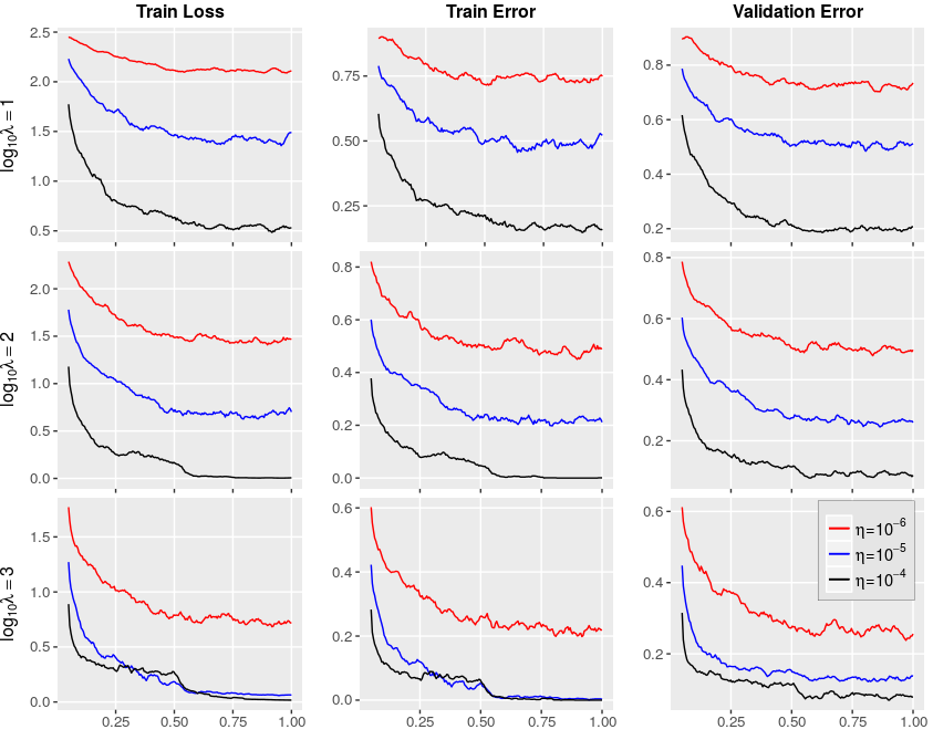
Figure 1: Performance of CG on ResNet-32 on CIFAR10 dataset ($x$-axis denotes the fraction of $T$): as $\lambda$ increases, the training error, loss value and test error all start to decrease simultaneously. Note that if $\lambda$ is sufficiently large (not over constraining the network), training and test errors start to go down significantly faster for a wide range of stepsizes $\eta$, showing that CG is stable under $\eta$.

Path-CG Algorithm: In order to simplify the presentation, we will assume that there are no biases noting that the procedure can be easily extended to the case when we have individual bias for every node. Let us fix a layer $j$ and the vectorized weight matrix of that layer be ${W}$ that we want to update and as usual, ${g}$ corresponds to the gradient. Let the number of nodes in the $(j-1)$ and $j$-th layers be $n_{1}$ and $n_{2}$ respectively. For each edge between these two layers we will compute the scaling factors $\gamma_{e}$ defined as,

$$\gamma_{e}=\sum_{v_{in}[i]\cdots\xrightarrow{e}\cdots v_{out}[j]}\left|\prod_{e_{k}\neq e}W_{e_{k}}\right|^{2}.$$ (13)

Intuitively, $\gamma_{e}$ computes the norm of all paths that pass through the edge $e$ excluding the weight of $e$. This can be efficiently done using Dynamic Programming in time $O(l)$ where $l$ is the number of layers. Consequently, the computation of path norm also satisfies the same runtime, see Neyshabur et al. (2015a) for more details. Now, observe that the path norm constraint when all of the other layers are fixed reduces to solving the following problem (the detailed derivation is in the supplement),

$$\min_{W}g^{T}W~{}\text{s.t.}~{}\|\Gamma W\|_{2}\leq\lambda$$ (14)

where $\Gamma$ is a diagonal matrix with $\Gamma_{e,e}=\gamma_{e}$, see (13). Hence, we can see that the problem again reduces to a simple rescaling and then normalization as seen for the Frobenius norm in (7) and repeat for each layer.

Remark 7

The starting point $W_{0}$ such that $\|W_{0}\|_{\pi}\leq\lambda$ can be chosen simply by randomly assigning the weights from the Normal Distribution with mean $0$.

Complexity of Path-CG 1: From the above discussion, our full algorithm is given in Algorithm 1. The main computational complexity in Path-CG comes from computing the matrix $\Gamma$ for each layer, but as we described earlier, this can be done by backpropagation. Hence, the complexity of our algorithm for running $T$ iterations is essentially $O(lBT)$ where $B$ is a size of the mini-batch.

Scale invariance of Path-CG 1: Note that CG algorithms satisfy a much general property called as Affine Invariance Jaggi (2013), which implies that it is also scale invariant. Scale invariance makes our algorithm more efficient (in wall clock time) since it avoids exploring functions that compute the value.

6 Experimental Evaluation

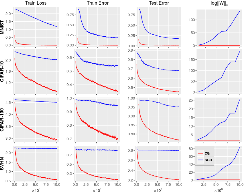
Figure 2: Performance of Path-CG vs SGD on a 2-layer fully connected network on four datasets (x-axis denotes the $\#$iterations). Observe that across all datasets, Path-CG is much faster than SGD (first three columns). Last column shows that SGD is not stable with respect to the path norm.

We present experimental results on three different case studies to support our basic premise and theoretical findings in the earlier sections: constraints can be easily handled with our CG algorithm in the context of Deep Learning while preserving the empirical performance of the models. The first set of experiments is designed to show how simple/generic constraints can be easily incorporated in existing deep learning models to get both faster training times and better accuracy while reducing the #-layers using the ResNet architecture. The second set of experiments is to evaluate our Path-CG algorithm. The goal is to show that Path-CG is much more stable than the Path-SGD algorithm in Neyshabur et al. (2015a), implying lower generalization error of the model. In the third set of experiments we show that GANs (Generative Adversarial Networks) can be trained faster using the CG algorithm and that the training tends to be stable. To validate this, we test the performance of the GAN on an image inpainting application. Since CG algorithm maintains a solution that is a convex combination of all previous iterates, hence to decrease the effect of random initialization, the training scheme consists of two phases: (i) burn-in phase in which the CG algorithm is run with a constant stepsize; (ii) decay phase in which the stepsize is decaying according to $1/t$. This makes sure that the effect of randomness from the initialization is diminished. We use $1$ epoch for the burn-in phase, hence we can conclude that the algorithm is guaranteed to converge to a stationary pointLacoste-Julien (2016).

6.1 Improve ResNets using Conditional Gradients

We start with the problem of image classification, detection and localization. For these tasks, one of the best performing architectures are variants of the Deep Residual Networks (ResNet) He et al. (2016). For our purposes, to analyze the performance of CG algorithm, we used the shallower variant of ResNet, namely ResNet-32 (32 hidden layers) architecture and trained on the CIFAR10 Krizhevsky et al. (2012) dataset. ResNet-32 consists of $5$ residual blocks and $2$ fully connected, one each at the input and output layers. Each residual block consists of 2 convolution, ReLu (Rectified Linear units), and batch normalization layers, see He et al. (2016) for more details. CIFAR10 dataset contains $60000$ color images of size $32\times 32$ with $10$ different categories/labels. Hence, the network contains approximately $0.46M$ parameters.

To make the discussion clear, we present results for the case where the total Frobenius norm of the network parameters is constrained to be less than $\lambda$ and trained using the CG algorithm. To see the effect of the parameters $\lambda$ and step sizes $\eta$ on the model, we ran $80000$ iterations, see Figure 1. The plots essentially show that if $\lambda$ is chosen big enough, then the accuracy of CG is very close to the accuracy of ResNet-164 ($5.46\%$ top-1 test error, see He et al. (2016)) that has many more parameters (approximately 5 times!). This is an interesting property with immediate practical import and shows that CG can be used to improve the performance of existing architectures by appropriately choosing constraints (see supplement for more experiments).

Takeaway: CG offers fewer parameters and higher accuracy on a standard network with no additional change.

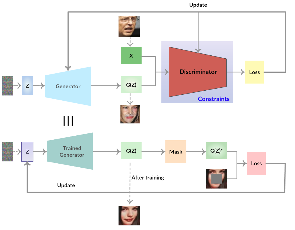
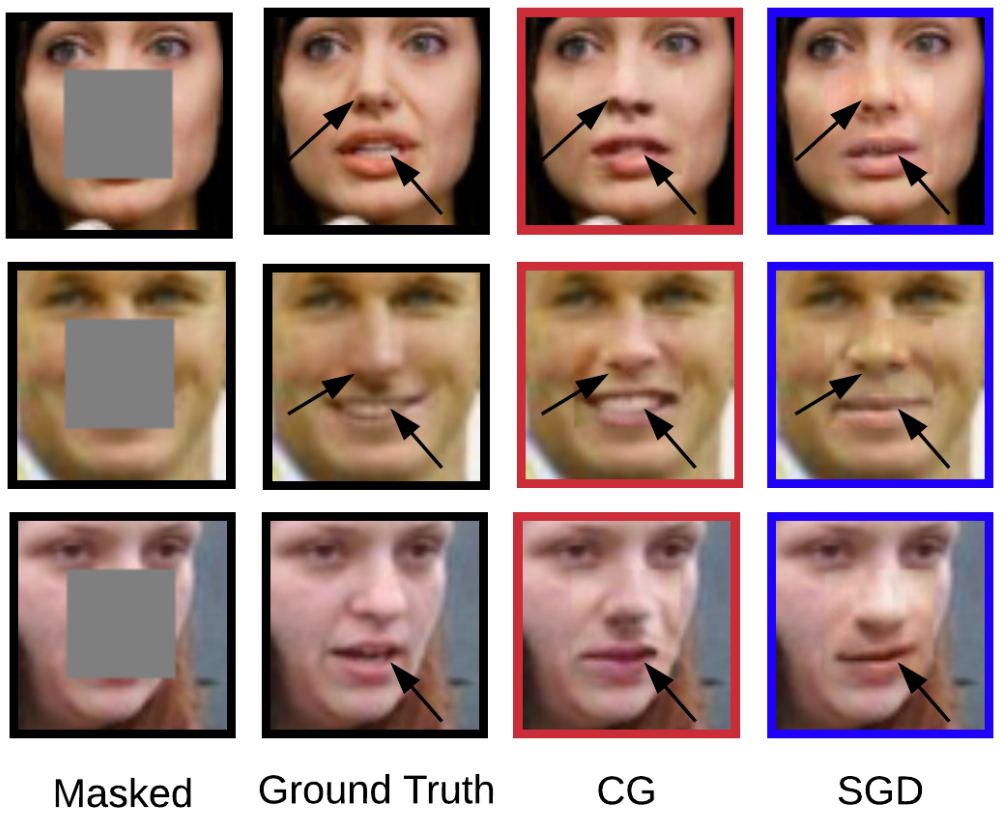
Figure 3: Left: Illustrates the task of image inpainting overall pipeline. Right: CG-trained DC-GAN performs as good as (or better than) SGD-based DC-GAN but with $50\%$ epochs (more qualitative results are provided in the supplement).

6.2 Path-CG vs Path-SGD: Which is better?

In this case study, the goal is to compare Path-CG with the Path-SGD algorithm Neyshabur et al. (2015a) in terms of both accuracy and stability of the algorithm. To that end, we considered image classification problem with a path norm constraint on the network: $\|W_{t}\|_{p}\leq\lambda$ for varying $\lambda$ as before. We train a simple feed-forward network which consists of $2$ fully-connected hidden layers with $4000$ units each, followed by the output layer with $10$ nodes. We used ReLu nonlinearity as the activation function and cross entropy as the loss, see Neyshabur et al. (2015a) for more details.
We performed experiments on 4 standard datasets for image classification: MNIST LeCun et al. (1998), CIFAR (10,100) Krizhevsky et al. (2012) and finally color images of house numbers from SVHN dataset Netzer et al. . Figure 2 shows the result for $\lambda=10^{6}$ (after tuning), it can achieve the same accuracy as that of Path-SGD.

Path-CG has one main advantage over Path-SGD: our results in the supplement that Path-CG is more stable while the path norm of Path-SGD algorithm increases rapidly. This shows that Path-SGD does not effectively regularize the path norm whereas Path-CG keeps the path norm less than $\lambda$ as expected.

Takeaway: All statistical benefits of path norm are possible via CG and at the same time computationally more stable.

6.3 Image Inpainting using Conditional Gradients

Finally, we illustrate the ability of our CG framework on an exciting and recent application of image inpainting using Generative Adversarial Networks (GANs). We now briefly explain the overall experimental setup. GANs using game theoretic notions can be defined as a system of 2 neural networks called Generator and the Discriminator competing with each other in a zero-sum game Arora et al. (2017).

Image inpainting/completion can be performed using the following two steps Amos : (i) Train a standard GAN as a normal image generation task, and (ii) use the trained generator and then tune the noise that gives the best output, see Figure 3 (left). Hence, our basic hypothesis is that if the generator is trained well, then the follow-up task of image inpainting benefits automatically.

Train DC-GAN faster for better image inpainting: We used the state of the art DC-GAN architecture in our experiments and we impose a Frobenius norm constraint on the parameters but only on the Discriminator to avoid mode collapse issues and trained using the CG algorithm. In order to verify the performance of the CG algorithm, we used 2 standard face image datasets from CelebA and LWF and conducted two experiments: trained on the CelebA dataset with LFW being the test dataset and vice-versa. The results are shown in Figure 3 (right) after tuning $\lambda$. We found that the generator generates very high quality images after being trained with LFW images in comparison to the original DC-GAN in just $10$ epochs (reducing the computational cost by $50\%$), figure 3 shows that the images completed using the CG trained DC-GAN look realistic. Our results indicate that CG trained DC-GAN qualitatively performs as good or better than the standard DC-GAN. Experiments showing the stability of our model with varying $\lambda$’s is in the supplement.

Takeaway: GANs can be trained faster with no change in accuracy.

7 Conclusions

The main emphasis of our work is to provide evidence supporting three distinct but related threads: (i) global constraints are relevant in the context of training deep models in vision and machine learning; (ii) the lack of support for global constraints in existing libraries like Keras and Tensorflow Abadi et al. (2016) may be because of the complex interplay between constraints and SGD which we have shown can be side-stepped, to a great extent, using CG; and (iii) constraints can be easily incorporated with negligible to small changes to existing implementations. We provide a range of empirical results on three different case studies to support our claims, and conjecture that a broad variety of other problems will immediately benefit by viewing them through the lens of conditional gradient algorithms. Our analysis and experiments suggest concrete ways in which one may realize performance improvements, in both generalization and runtime, by substituting in CG schemes in certain classes of deep learning models. Tensorflow code for all our experiments will be made available in Github.

Appendix

8 Dealing with Category 2 Constraints more efficiently

Let $\|W\|_{s,p}:=\|\left(\|W_{1}\|,\|W_{2}\|,...,\|W_{l}\|\right)\|_{p}$ be the $\ell_{s,p}$ norm of $W$ where $W_{i}$ be the weight matrix corresponding to edges between layer $i-1$ and $i$. Then $\ell_{1}/\ell_{\infty}$ norm is defined as $\|W\|_{1,\infty}:=\max_{i}|W_{i}|_{1}$. Then we need to solve the following at each iteration:

$$\{s_{i}\}\in\arg\min_{W_{i}}\sum_{i=1}^{l}\langle G_{i},W_{i}\rangle\quad\text{s.t.}\quad\max_{i}|W_{i}|_{1}\leq\lambda.$$ (15)

Now it is easy to see that we set that the optimal solution can be computed as follows. For each (gradient) matrix $G_{i}$ we simply compute the element (or index) with the maximum magnitude. We then set the corresponding index to $\lambda$ if the sign of the gradient in that index is negative and vice-versa. This procedure updates $l$ elements in each iteration. We can similarly switch the roles of the max function, absolute function and define the $\ell_{\infty}/\ell_{1}$ norm which will lead to updating one layer at each iteration. For more specific group norms see Garber and Hazan (2015). Specifically, for matrix induced group norms, lemma 9 in Garber and Hazan (2015) shows that the corresponding linear optimization problem at each iteration can be solved efficiently.

9 Proof of Lemma 4.1.

Lemma 8

An $\epsilon$-approximate CG step for the TV norm can be computed in $O(1/\epsilon)$ time (independent of dimensions of $A\in\mathbb{R}^{n\times E}$).

Proof  Harchaoui et al. (2015) showed that in order to solve the CG step for TV norm we first solve

$$\max_{\beta\in\mathbb{R},f}\beta~{}\text{s.t.}~{}Af=\beta g_{t},f\in[0,1]^{E},$$ (16)

where $E$ is the number of edges of the network and then compute the Lagrange multipliers at the optimal solution of problem (16). Instead of first solving (16), we propose to solve the dual directly using continuous optimization techniques. Introducing dual variables $v$ for the equality constraints and $w$ for the box constraints, our dual linear program can be written as,

$$\max_{w,v}1^{T}w\quad\text{s.t.}\quad-A^{T}v+w\leq 0,~{}g_{t}^{T}v=-1,~{}w\leq 0.$$ (17)

Since $v$ is a free variable, problem (17) is equivalent to,

$$\max_{w,v}1^{T}w\quad\text{s.t.}\quad w\leq A^{T}v,~{}g_{t}^{T}v=1,~{}w\leq 0.$$ (18)

Eliminating $w$, we can write the dual of (16) as,

$$\min_{v\in\mathbb{R}^{E}}\sum_{i=1}^{E}\min\left(0,v^{T}A_{[i,:]}\right)~{}\text{s.t.}~{}g_{t}^{T}v=1$$ (19)

where $A_{[i,:]}$ denotes the $i$-th row of $A$. Now it is easy to see that many continuous optimization methods are amenable which does not require us to instantiate the matrix $A$. Hence we can now use Theorem 1 in Johnson and Zhang (2013) gives us the desired result.  

10 Path-CG

In this section we provide details on the Path-CG updates in Section 5 of the main paper.

Figure 4: In order to compute the path norm, we can compute $\gamma_{in}$ and $\gamma_{out}$ for each node in the network. We then set $\gamma(u\to v)=\gamma_{in}(u)\gamma_{out}(v)$

Define $\gamma_{in}(v)$ and $\gamma_{out}(v)$ as,

$$\gamma_{in}(v)=\sum_{(u\to v)\in E}\gamma_{in}(u)w_{u,v}^{2}$$ (20)

$$\gamma_{out}(v)=\sum_{(v\to u)\in E}\gamma_{out}(u)w_{u,v}^{2}$$ (21)

Fix layer $i$ that we want to update and let the $g_{i}^{t}$ be the gradient of the loss function with respect to the weight matrix of the edges between $i-1$ and $i$ layers. Then the squared path norm can be computed as the sum of squares (taken over all edges) of product of $\gamma_{uv}:=\gamma_{in}(u)\gamma_{out}(v)$ and $w_{uv}^{2}$ for every edge in between the layers, that is,

$$\|W\|_{\pi}^{2}:=\sum_{uv}\gamma_{uv}w_{uv}^{2}=\|\hat{\Gamma}W\|_{F}^{2}$$ (22)

where the matrix $\hat{\Gamma}$ is diagonal with elements being $\gamma_{uv}^{1/2}$. Hence we have that the Path-CG subproblems correspond to solving

$$\min_{W}g^{T}W\quad\text{s.t.}\quad\|\hat{\Gamma}W\|_{2}\leq\lambda$$ (23)

as shown in the main section.

References

- Abadi et al. (2016) Martín Abadi, Ashish Agarwal, Paul Barham, Eugene Brevdo, Zhifeng Chen, Craig Citro, Greg S Corrado, Andy Davis, Jeffrey Dean, Matthieu Devin, et al. Tensorflow: Large-scale machine learning on heterogeneous distributed systems. arXiv preprint arXiv:1603.04467, 2016.
- (2) Brandon Amos. Image Completion with Deep Learning in TensorFlow. http://bamos.github.io/2016/08/09/deep-completion. Accessed: [11/15/2017].
- Arora et al. (2017) Sanjeev Arora, Rong Ge, Yingyu Liang, Tengyu Ma, and Yi Zhang. Generalization and equilibrium in generative adversarial nets (gans). In International Conference on Machine Learning, 2017.
- Bach et al. (2012) Francis Bach, Rodolphe Jenatton, Julien Mairal, Guillaume Obozinski, et al. Optimization with sparsity-inducing penalties. Foundations and Trends® in Machine Learning, 2012.
- Barone (2016) Antonio Valerio Miceli Barone. Low-rank passthrough neural networks. arXiv preprint arXiv:1603.03116, 2016.
- Bengio (2012) Yoshua Bengio. Practical recommendations for gradient-based training of deep architectures. In Neural networks: Tricks of the trade, pages 437–478. Springer, 2012.
- Boyd and Vandenberghe (2004) Stephen Boyd and Lieven Vandenberghe. Convex optimization. Cambridge university press, 2004.
- Cai et al. (2010) Jian-Feng Cai, Emmanuel J Candès, and Zuowei Shen. A singular value thresholding algorithm for matrix completion. SIAM Journal on Optimization, 2010.
- Chambolle and Lions (1997) Antonin Chambolle and Pierre-Louis Lions. Image recovery via total variation minimization and related problems. Numerische Mathematik, 1997.
- Charles (2013) P.W.D. Charles. Project title. https://github.com/charlespwd/project-title, 2013.
- Cheng et al. (2017) Yu Cheng, Duo Wang, Pan Zhou, and Tao Zhang. A survey of model compression and acceleration for deep neural networks. arXiv preprint arXiv:1710.09282, 2017.
- Collins and Kohli (2014) Maxwell D Collins and Pushmeet Kohli. Memory bounded deep convolutional networks. arXiv preprint arXiv:1412.1442, 2014.
- Dauphin et al. (2015) Yann Dauphin, Harm de Vries, and Yoshua Bengio. Equilibrated adaptive learning rates for non-convex optimization. In Advances in neural information processing systems, pages 1504–1512, 2015.
- Defazio et al. (2014) Aaron Defazio, Francis Bach, and Simon Lacoste-Julien. Saga: A fast incremental gradient method with support for non-strongly convex composite objectives. In Advances in Neural Information Processing Systems, 2014.
- Duchi et al. (2008) John Duchi, Shai Shalev-Shwartz, Yoram Singer, and Tushar Chandra. Efficient projections onto the l 1-ball for learning in high dimensions. In Proceedings of the 25th international conference on Machine learning. ACM, 2008.
- Duchi et al. (2011) John Duchi, Elad Hazan, and Yoram Singer. Adaptive subgradient methods for online learning and stochastic optimization. Journal of Machine Learning Research, 2011.
- Fadili and Peyré (2011) Jalal M Fadili and Gabriel Peyré. Total variation projection with first order schemes. IEEE Transactions on Image Processing, 2011.
- Frank and Wolfe (1956) Marguerite Frank and Philip Wolfe. An algorithm for quadratic programming. Naval Research Logistics (NRL), 1956.
- Frerix et al. (2017) Thomas Frerix, Thomas Möllenhoff, Michael Moeller, and Daniel Cremers. Proximal backpropagation. arXiv preprint arXiv:1706.04638, 2017.
- Garber and Hazan (2015) Dan Garber and Elad Hazan. Faster rates for the frank-wolfe method over strongly-convex sets. In International Conference on Machine Learning, pages 541–549, 2015.
- Ghadimi and Lan (2013) Saeed Ghadimi and Guanghui Lan. Stochastic first-and zeroth-order methods for nonconvex stochastic programming. SIAM Journal on Optimization, 23(4):2341–2368, 2013.
- Goldfarb and Yin (2009) Donald Goldfarb and Wotao Yin. Parametric maximum flow algorithms for fast total variation minimization. SIAM Journal on Scientific Computing, 2009.
- Golub and Van Loan (2012) Gene H Golub and Charles F Van Loan. Matrix computations, volume 3. JHU Press, 2012.
- Grubb and Bagnell (2010) Alexander Grubb and J Andrew Bagnell. Boosted backpropagation learning for training deep modular networks. In Proceedings of the 27th International Conference on Machine Learning (ICML-10), pages 407–414, 2010.
- Haeffele and Vidal (2015) Benjamin D Haeffele and René Vidal. Global optimality in tensor factorization, deep learning, and beyond. arXiv preprint arXiv:1506.07540, 2015.
- Han et al. (2015) Song Han, Huizi Mao, and William J Dally. Deep compression: Compressing deep neural networks with pruning, trained quantization and huffman coding. arXiv preprint arXiv:1510.00149, 2015.
- Harchaoui et al. (2015) Zaid Harchaoui, Anatoli Juditsky, and Arkadi Nemirovski. Conditional gradient algorithms for norm-regularized smooth convex optimization. Mathematical Programming, 2015.
- Hardt et al. (2016) Moritz Hardt, Ben Recht, and Yoram Singer. Train faster, generalize better: Stability of stochastic gradient descent. In International Conference on Machine Learning, pages 1225–1234, 2016.
- He et al. (2016) Kaiming He, Xiangyu Zhang, Shaoqing Ren, and Jian Sun. Deep residual learning for image recognition. In Proceedings of the IEEE conference on computer vision and pattern recognition, 2016.
- Howard et al. (2017) Andrew G Howard, Menglong Zhu, Bo Chen, Dmitry Kalenichenko, Weijun Wang, Tobias Weyand, Marco Andreetto, and Hartwig Adam. Mobilenets: Efficient convolutional neural networks for mobile vision applications. arXiv preprint arXiv:1704.04861, 2017.
- Jaggi (2013) Martin Jaggi. Revisiting frank-wolfe: projection-free sparse convex optimization. In Proceedings of the 30th International Conference on International Conference on Machine Learning-Volume 28. JMLR. org, 2013.
- Janzamin et al. (2015) Majid Janzamin, Hanie Sedghi, and Anima Anandkumar. Beating the perils of non-convexity: Guaranteed training of neural networks using tensor methods. arXiv preprint arXiv:1506.08473, 2015.
- Johnson and Zhang (2013) Rie Johnson and Tong Zhang. Accelerating stochastic gradient descent using predictive variance reduction. In Advances in neural information processing systems, pages 315–323, 2013.
- Kingma and Ba (2014) Diederik Kingma and Jimmy Ba. Adam: A method for stochastic optimization. arXiv preprint arXiv:1412.6980, 2014.
- Krizhevsky et al. (2012) Alex Krizhevsky, Ilya Sutskever, and Geoffrey E Hinton. Imagenet classification with deep convolutional neural networks. In Advances in neural information processing systems, pages 1097–1105, 2012.
- Lacoste-Julien (2016) Simon Lacoste-Julien. Convergence rate of frank-wolfe for non-convex objectives. arXiv preprint arXiv:1607.00345, 2016.
- Lacoste-Julien and Jaggi (2015) Simon Lacoste-Julien and Martin Jaggi. On the global linear convergence of frank-wolfe optimization variants. In Advances in Neural Information Processing Systems, 2015.
- LeCun et al. (1998) Yann LeCun, Léon Bottou, Yoshua Bengio, and Patrick Haffner. Gradient-based learning applied to document recognition. Proceedings of the IEEE, 1998.
- Liu et al. (2015) Baoyuan Liu, Min Wang, Hassan Foroosh, Marshall Tappen, and Marianna Pensky. Sparse convolutional neural networks. In Proceedings of the IEEE Conference on Computer Vision and Pattern Recognition, 2015.
- Márquez-Neila et al. (2017) Pablo Márquez-Neila, Mathieu Salzmann, and Pascal Fua. Imposing hard constraints on deep networks: Promises and limitations. arXiv preprint arXiv:1706.02025, 2017.
- Mikolov et al. (2014) Tomas Mikolov, Armand Joulin, Sumit Chopra, Michael Mathieu, and Marc’Aurelio Ranzato. Learning longer memory in recurrent neural networks. arXiv preprint arXiv:1412.7753, 2014.
- Mundle (1959) CWK Mundle. Probability and scientific inference. Philosophy, 1959.
- (43) Yuval Netzer, Tao Wang, Adam Coates, Alessandro Bissacco, Bo Wu, and Andrew Y Ng. Reading digits in natural images with unsupervised feature learning.
- Neyshabur et al. (2015a) Behnam Neyshabur, Ruslan R Salakhutdinov, and Nati Srebro. Path-sgd: Path-normalized optimization in deep neural networks. In Advances in Neural Information Processing Systems, 2015a.
- Neyshabur et al. (2015b) Behnam Neyshabur, Ryota Tomioka, and Nathan Srebro. Norm-based capacity control in neural networks. In Conference on Learning Theory, 2015b.
- Oktay et al. (2017) Ozan Oktay, Enzo Ferrante, Konstantinos Kamnitsas, Mattias Heinrich, Wenjia Bai, Jose Caballero, Ricardo Guerrero, Stuart Cook, Antonio de Marvao, Declan O’Regan, et al. Anatomically constrained neural networks (acnn): Application to cardiac image enhancement and segmentation. arXiv preprint arXiv:1705.08302, 2017.
- Pathak et al. (2015) Deepak Pathak, Philipp Krahenbuhl, and Trevor Darrell. Constrained convolutional neural networks for weakly supervised segmentation. In Proceedings of the IEEE International Conference on Computer Vision, pages 1796–1804, 2015.
- Platt and Barr (1988) John C Platt and Alan H Barr. Constrained differential optimization. In Neural Information Processing Systems, pages 612–621, 1988.
- Raginsky et al. (2017) Maxim Raginsky, Alexander Rakhlin, and Matus Telgarsky. Non-convex learning via stochastic gradient langevin dynamics: a nonasymptotic analysis. arXiv preprint arXiv:1702.03849, 2017.
- Recht et al. (2010) Benjamin Recht, Maryam Fazel, and Pablo A Parrilo. Guaranteed minimum-rank solutions of linear matrix equations via nuclear norm minimization. SIAM review, 2010.
- Reddi et al. (2016) Sashank J Reddi, Suvrit Sra, Barnabás Póczos, and Alex Smola. Stochastic frank-wolfe methods for nonconvex optimization. In Communication, Control, and Computing (Allerton), 2016 54th Annual Allerton Conference on, 2016.
- Rissanen (1985) Jorma Rissanen. Minimum description length principle. Wiley Online Library, 1985.
- Rudd et al. (2014) Keith Rudd, Gianluca Di Muro, and Silvia Ferrari. A constrained backpropagation approach for the adaptive solution of partial differential equations. IEEE transactions on neural networks and learning systems, 2014.
- Ruder (2017) Sebastian Ruder. An overview of multi-task learning in deep neural networks. arXiv preprint arXiv:1706.05098, 2017.
- Soudry and Carmon (2016) Daniel Soudry and Yair Carmon. No bad local minima: Data independent training error guarantees for multilayer neural networks. arXiv preprint arXiv:1605.08361, 2016.
- Srivastava et al. (2014) Nitish Srivastava, Geoffrey E Hinton, Alex Krizhevsky, Ilya Sutskever, and Ruslan Salakhutdinov. Dropout: a simple way to prevent neural networks from overfitting. Journal of machine learning research, 2014.
- Tai et al. (2015) Cheng Tai, Tong Xiao, Yi Zhang, Xiaogang Wang, et al. Convolutional neural networks with low-rank regularization. arXiv preprint arXiv:1511.06067, 2015.
- Taylor et al. (2016) Gavin Taylor, Ryan Burmeister, Zheng Xu, Bharat Singh, Ankit Patel, and Tom Goldstein. Training neural networks without gradients: A scalable admm approach. In International Conference on Machine Learning, 2016.
- Tikhonov et al. (1987) Andre Nikolaevich Tikhonov, AV Goncharsky, and M Bloch. Ill-posed problems in the natural sciences. Mir Moscow, 1987.
- Wahba (1990) Grace Wahba. Spline models for observational data. SIAM, 1990.
- (61) Eric Wong and J Zico Kolter. Neural network inversion beyond gradient descent.
- Zeiler (2012) Matthew D Zeiler. Adadelta: an adaptive learning rate method. arXiv preprint arXiv:1212.5701, 2012.
- Zhang and Constantinides (1992) Shengwei Zhang and AG Constantinides. Lagrange programming neural networks. IEEE Transactions on Circuits and Systems II: Analog and Digital Signal Processing, 1992.