Datalog: Bag Semantics via Set Semantics

Abstract

Duplicates in data management are common and problematic. In this work, we present a translation of Datalog under bag semantics into a well-behaved extension of Datalog, the so-called warded Datalog^±, under set semantics. From a theoretical point of view, this allows us to reason on bag semantics by making use of the well-established theoretical foundations of set semantics. From a practical point of view, this allows us to handle the bag semantics of Datalog by powerful, existing query engines for the required extension of Datalog. This use of Datalog^± is extended to give a set semantics to duplicates in Datalog^± itself. We investigate the properties of the resulting Datalog^± programs, the problem of deciding multiplicities, and expressibility of some bag operations. Moreover, the proposed translation has the potential for interesting applications such as to Multiset Relational Algebra and the semantic web query language SPARQL with bag semantics.

1 Introduction

Duplicates are a common feature in data management. They appear, for instance, in the result of SQL queries over relational databases or when a SPARQL query is posed over RDF data. However, the semantics of data operations and queries in the presence of duplicates is not always clear, because duplicates are handled by bags or multisets, but common logic-based semantics in data management are set-theoretical, making it difficult to tell apart duplicates through the use of sets alone. To address this problem, a bag semantics for Datalog programs was proposed in [21], what we refer to as the derivation-tree bag semantics (DTB semantics). Intuitively, two duplicates of the same tuple in an intentional predicate are accepted as such if they have syntactically different derivation trees. The DTB semantics was used in [2] to provide a bag semantics for SPARQL.

The DTB semantics follows a proof-theoretic approach, which requires external, meta-level reasoning over the set of all derivation trees rather than allowing for a query language that inherently collects those duplicates. The main goal of this paper is to identify a syntactic class of extended Datalog programs, such that: (a) it extends classical Datalog with stratified negation and has a classical model-based semantics, (b) for every program in the class with a bag semantics, another program in the same class can be built that has a set-semantics and fully captures the bag semantics of the initial program, (c) it can be used in particular to give a set-semantics for classical Datalog with stratified negation with bag semantics. All these results can be applied, in particular, to multi-relational algebra, i.e. relational algebra with duplicates.

To this end, we show that the DTB semantics of a Datalog program can be represented by means of its transformation into a Datalog^± program [8, 10], in such a way that the intended model of the former, including duplicates, can be characterized as the result of the duplicate-free chase instance for the latter. The crucial idea of our translation from bag semantics into set semantics (of Datalog^±) is the introduction of tuple ids (tids) via existentially quantified variables in the rule heads. Different tids of the same tuple will allow us to identify usual duplicates when falling back to a bag semantics for the original Datalog program. We establish the correspondence between the DTB semantics and ours. This correspondence is then extended to Datalog with stratified negation. We thus recover full relational algebra (including set difference) with bag semantics in terms of a well-behaved query language under set semantics.

The programs we use for this task belong to warded Datalog^± [17]. This is a particularly well-behaved class of programs in that it properly extends Datalog, has a tractable conjunctive query answering (CQA) problem, and has recently been implemented in a powerful query engine, namely the VADALOG System [6, 7]. None of the other well-known classes of Datalog^± share these properties: for instance, guarded [8], sticky and weakly-sticky [11] Datalog^± only allow restricted forms of joins and, hence, do not cover Datalog. On the other hand, more expressive languages, such as weakly frontier guarded Datalog^± [5], lose tractability of CQA. Warded Datalog^± has been successfully applied to represent a core fragment of SPARQL under certain OWL 2 QL entailment regimes [16], with set semantics though [17] (see also [3, 4]), and it looks promising as a general language for specifying different data management tasks [6].

We then go one step further and also express the bag semantics of Datalog^± by means of the set semantics of Datalog^±. In fact, we show that the bag semantics of a very general language in the Datalog^± class can be expressed via the set semantics of Datalog^± and the transformed program is warded whenever the initial program is.

Structure and main results. In Section 2, we recall some basic notions. In Section 7, we conclude and discuss some future extensions. The main results of the paper are detailed in Sections 3 – 6.

• Our translation of Datalog with bag semantics into warded Datalog^± with set semantics, which will be referred to as program-based bag (PBB ) semantics, is presented in Section 3. We also show how this translation can be extended to Datalog with stratified negation.

• In Section 4, we study the transformation from bag semantics into set semantics for Datalog^± itself. We thus carry over both the DTB semantics and the PBB semantics to Datalog^± with a form of stratified negation, and establish the equivalence of these two semantics also for this extended query language. Moreover, we verify that the Datalog^± programs resulting from our transformation are warded whenever the programs to start with belong to this class.

• In Section 5, we study crucial decision problems related to multiplicities. Above all, we are interested in the question if a given tuple has finite or infinite multiplicity. Moreover, in case of finiteness, we want to compute the precise multiplicity. We show that these tasks can be accomplished in polynomial time (data complexity).

• In Section 6, we apply our results on Datalog with bag semantics to Multiset Relational Algebra (MRA). We also discuss alternative semantics for multiset-intersection and multiset-difference, and the difficulties to capture them with our Datalog^± approach.

2 Preliminaries

We assume familiarity with the relational data model, conjunctive queries (CQs), in particular Boolean conjunctive queries (BCQs); classical Datalog with minimal-model semantics, and Datalog with stratified negation with standard-model semantics, denoted Datalog^¬s (see [1] for an introduction). An $n$-ary relational predicate $P$ has positions: $P[1],\ldots,P[n]$. With ${\it Pos}(P)$ we denote the set of positions of predicate $P$; and with ${\it Pos}(\Pi)$ the set of positions of (predicates in) a program $\Pi$.

2.1 Derivation-Tree Bag (DTB) Semantics for Datalog and Datalog^¬s

We follow [21], where tuples are colored to tell apart duplicates of a same element in the extensional database (EDB), via an infinite, ordered list $\mathcal{C}$ of colors  $c_{1},c_{2},\ldots$. For a multiset $M$,  $e\in M$ if ${\it mult}(e,M)>0$ holds, where ${\it mult}(e,M)$ denotes the multiplicity of $e$ in $M$. In this case, the $n$ copies of $e$ are denoted by $e\!\!:\!\!{1},\ldots,e\!\!:\!\!{n}$, indicating that they are colored with $c_{1},\ldots,c_{n}$, respectively. So, ${\it col}(e):=\{e\!\!:\!\!{1},\ldots,e\!\!:\!\!{n}\}$ becomes a set. A multiset $M_{1}$ is (multi)contained in multiset $M_{2}$, when ${\it mult}(e,M_{1})\leq{\it mult}(e,M_{2})$ for every $e\in M_{1}$. For a multiset $M$, ${\it col}(M):=\bigcup_{e\in M}{\it col}(e)$, which is a set. For a “colored" set $S$, ${\it col}^{-1}(S)$ produces a multiset by stripping tuples from their colors.

Example 2.1.

For $M=\{a,a,a,b,b,c\}$, ${\it col}(a)=\{a\!\!:\!\!{1},a\!\!:\!\!{2},a\!\!:\!\!{3}\}$, and ${\it col}(M)=S=\{a\!\!:\!\!{1},a\!\!:\!\!{2},a\!\!:\!\!{3},b\!\!:\!\!{1},b\!\!:\!\!{2},c\!\!:\!\!{1}\}$. The inverse operation, the decoloration, gives, for instance: ${\it col}^{-1}(a\!\!:\!\!{2}):=a$; and ${\it col}^{-1}(S):=\{a,a,a,b,b,c\}$, a multiset. $\Box$

We consider Datalog programs $\Pi$ with multiset predicates and multiset EDBs $D$. A derivation tree (DT) for $\Pi$ wrt. $D$ is a tree with labeled nodes and edges, as follows:

1. For an EDB predicate $P$ and $h\in{\it col}(P(D))$, a DT for ${\it col}^{-1}(h)$ contains a single node with label $h$.

2. For each rule of the form  $\rho\!:\ H\leftarrow A_{1},A_{2},\ldots,A_{k}$;   with $k>0$,  and each tuple $\langle{\mathcal{T}}_{1},\ldots,{\mathcal{T}}_{k}\rangle$ of DTs for the atoms $\langle d_{1},\ldots,d_{k}\rangle$ that unify with $\langle A_{1},A_{2},\ldots,A_{k}\rangle$ with mgu $\theta$, generate a DT for $H\theta$ with $H\theta$ as the root label, $\langle{\mathcal{T}}_{1},\ldots,{\mathcal{T}}_{k}\rangle$ as the children, and $\rho$ as the label for the edges from the root to the children. We assume that these children are arranged in the order of the corresponding body atoms in rule $\rho$.

For a DT ${\mathcal{T}}$, we define ${\it Atoms}({\mathcal{T}})$ as ${\it col}^{-1}$ of the root when ${\mathcal{T}}$ is a single-node tree, and the root-label of ${\mathcal{T}}$, otherwise. For a set of DTs $\mathfrak{T}$:  ${\it Atoms}(\mathfrak{T}):=\biguplus\{{\it Atoms}({\mathcal{T}})\leavevmode\nobreak\ |\leavevmode\nobreak\ {\mathcal{T}}\in\mathfrak{T}\}$, which is a multiset that multi-contains $D$. Here, we write $\biguplus$ to denote the multi-union of (multi)sets that keeps all duplicates. If ${\it DT}(\Pi,$ ${\it col}(D))$ is the set of (syntactically different) DTs, the derivation-tree bag (DTB) semantics for $\Pi$ is the multiset   ${\it DTBS}(\Pi,D):={\it Atoms}({\it DT}(\Pi,{\it col}(D)))$. (Cf. [18] for an equivalent, provenance-based bag semantics for Datalog.)

$P(1,2)$

$\rho_{1}$ $R(1,2)$ $\rho_{2}$ $Q(1,2,3)\!:\!1$ $\rho_{1}$      $S(1,2)$ $\rho_{3}$      $T(4,1,2)\!:\!1$

$P(1,2)$

$\rho_{1}$ $R(1,2)$ $\rho_{2}$ $Q(1,2,5)\!:\!1$ $\rho_{1}$      $S(1,2)$ $\rho_{3}$      $T(4,1,2)\!:\!1$

$P(1,2)$

$\rho_{1}$ $R(1,2)$ $\rho_{2}$ $Q(1,2,3)\!:\!1$ $\rho_{1}$      $S(1,2)$ $\rho_{3}$      $T(4,1,2)\!:\!2$

Figure 1: Three (out of four) derivation-trees for $P(1,2)$ in Example 2.2.

Example 2.2.

Consider the program $\Pi=\{\rho_{1},\rho_{2},\rho_{3}\}$ and multiset EDB $D=\{Q(1,2,3)$, $Q(1,2,5),Q(2,3,4),Q(2,3,4),T(4,1,2),T(4,1,2)\}$, where $\rho_{1},\rho_{2},\rho_{3}$ are defined as follows:
     $\rho_{1}\!:\ P(x,y)\leftarrow R(x,y),S(x,y)$;  $\rho_{2}\!:\ R(x,y)\leftarrow Q(x,y,z)$;  $\rho_{3}\!:\ S(x,y)\leftarrow T(z,x,y).$

Here, ${\it col}(D)=\{Q(1,2,3)\!\!:\!\!{1},Q(1,2,5)\!\!:\!\!{1},Q(2,3,4)\!\!:\!\!{1},Q(2,3,4)\!\!:\!\!{2},T(4,1,2)\!\!:\!\!{1},T(4,1,2)\!\!:\!\!{2}\}$. In total, we have 16 DTs:  (a) 6 single-node trees with labels in ${\it col}(D)$ (b) 6 depth-two, linear trees (root to the left, i.e. rotated in $-90^{\circ}$): $R(1,2)-$ $\rho_{2}-Q(1,2,3)\!\!:\!\!{1}$. $R(1,2)-\rho_{2}-{Q(1,2,5)\!\!:\!\!{1}}$. $R(2,3)-\rho_{2}-Q(2,3,4)\!\!:\!\!{1}$. $R(2,3)-\rho_{2}-Q(2,3,4)\!\!:\!\!{2}$. $S(1,2)-\rho_{3}-T(4,1,2)\!\!:\!\!{1}$. $S(1,2)-\rho_{3}-T(4,1,2)\!\!:\!\!{2}$. (c) 4 depth-three trees for $P(1,2)$, three of which are displayed in Figure 1. The 16 different DTs in ${\it DT}(\Pi,{\it col}(D))$ give rise to ${\it DTBS}(\Pi,D)=D\ \cup\ \{R(1,2),$ $R(1,2),$ $R(2,3)$, $R(2,3),$ $S(1,2)$, $S(1,2),$ $P(1,2),$ $P(1,2),$ $P(1,2),$ $P(1,2)\}$. $\Box$

In [22], a bag semantics for Datalog^¬s was introduced via derivation-trees (DTs), extending the DTB semantics in [21] for (positive) Datalog. This extension applies to Datalog programs with stratified negation that are range-restricted and safe, i.e. a variable in a rule head or in a negative literal must appear in a positive literal in the body of the same rule. (The semantics in [22] does not consider duplicates in the EDB, but it is easy to extend the DTB semantics with multiset EDBs using colorings as above.)  If $\Pi$ is a Datalog^¬s program with multiset predicates and multiset EDB $D$, a derivation tree for $\Pi$ wrt. $D$ is as for Datalog programs, but with condition 2. modified as follows:

• Now let $\rho$ be a rule of the form $\rho\!:\ H\leftarrow A_{1},A_{2},\ldots,A_{k},\neg B_{1},\dots\neg B_{\ell}$;   with $k>0$ and $\ell\geq 0$. Let the predicate of $H$ be of some stratum $i$ and let the predicates of $B_{1},\dots,B_{\ell}$ be of some stratum $<i$. Assume that we have already computed all derivation trees for (atoms with) predicates up to stratum $i-1$. Then, for each tuple $\langle{\mathcal{T}}_{1},\ldots,{\mathcal{T}}_{k}\rangle$ of DTs for the atoms $\langle d_{1},\ldots,d_{k}\rangle$ that unify with $\langle A_{1},A_{2},\ldots,A_{k}\rangle$ with mgu $\theta$, such that there is no DT for any of the atoms $B_{1}\theta,\dots,B_{\ell}\theta$, generate a DT for $H\theta$ with $H\theta$ as the root label and $\langle{\mathcal{T}}_{1},\ldots,{\mathcal{T}}_{k},\neg B_{1}\theta,\dots,\neg B_{\ell}\theta\rangle$ as the children, in this order. Furthermore, all edges from the root to its children are labelled with $\rho$.

Analogously to the positive case, now for a range-restricted and safe program $\Pi$ in Datalog^¬s and multiset EDB $D$, we write ${\it DTBS}(\Pi,D)$ to denote the derivation-tree based bag semantics.

Example 2.3.

(ex. 2.2 cont.) Consider now the EDB $D^{\prime}=\{Q(1,2,3)$, $Q(1,2,5),Q(2,3,4),$ $Q(2,3,4),T(4,1,2)\}$ (with one duplicate of $T(4,1,2)$ removed from $D$), and modify $\Pi$ to $\Pi^{\prime}=\{\rho^{\prime}_{1},\rho_{2},\rho_{3}\}$ with $\rho^{\prime}_{1}\!:\ \ P(x,y)\leftarrow R(x,y),\neg S(x,y)$  (i.e., $\rho^{\prime}_{1}$ now encodes multiset difference).  Then, predicates $Q,R,S,T$ are on stratum 0 and $P$ is on stratum 1. The DTs for atoms with predicates from stratum 0 are as in Example 2.2 with two exceptions: there is now only one single-node DT for $T(4,1,2)$ and only one DT for $S(1,2)$.

For ground atoms with predicate $P$, we now only get two DTs producing $P(2,3)$. One of them is shown in Figure 2 on the left-hand side. The other DT of $P(2,3)$ is obtained by replacing the left-most leave $Q(2,3,4)\!\!:\!\!1$ by $Q(2,3,4)\!\!:\!\!2$. In particular, the DT of $P(2,3)$ in Figure 2 shows that the “derivation” of $\neg S(2,3)$ succeeds, i.e., there is no DT for $S(2,3)$. The remaining two trees in Figure 2 establish that $P(2,3)$ do not have a DT because $S(1,2)$ does have a DT. In total, we have 12 different DTs in ${\it DT}(\Pi^{\prime},{\it col}(D^{\prime}))$ with ${\it DTBS}(\Pi^{\prime},D^{\prime})=D^{\prime}\ \cup\ \{R(1,2),$ $R(1,2),$ $R(2,3),$ $R(2,3),$ $S(1,2),$ $P(2,3),$ $P(2,3)\}$.

Notice that the DT semantics interprets the difference in rule $\rho_{1}^{\prime}$ as “all or nothing": when computing $P(x,y)$, a single DT for $S(x,y)$ “kills" all the DTs for $R(x,y)$  (cf. Section 6). For example, $P(1,2)$ is not obtained despite the fact that we have two copies of $R(1,2)$ and only one of $S(1,2)$, as the two trees on the right-hand side in Figure 2 show. $\Box$

$P(2,3)$

$\rho_{1}$ $R(2,3)$ $\rho_{2}$ $Q(2,3,4)\!:\!1$ $\rho_{1}$ $\stackrel{{\scriptstyle\neg S(2,3){\Large\ \surd}}}{{\not\exists{\it DT}\mbox{ for }S(2,3)?}}$ succeeds

$P(1,2)$

$\rho_{1}$ $R(1,2)$ $\rho_{2}$ $Q(1,2,3)\!:\!1$ $\rho_{1}$      $\stackrel{{\scriptstyle\neg S(1,2){\Large\ \times}}}{{\not\exists{\it DT}\mbox{ for }S(1,2)?}}$ fails

$P(1,2)$

$\rho_{1}$ $R(1,2)$ $\rho_{2}$ $Q(1,2,5)\!:\!1$ $\rho_{1}$      $\stackrel{{\scriptstyle\neg S(1,2){\Large\ \times}}}{{\not\exists{\it DT}\mbox{ for }S(1,2)?}}$ fails

Figure 2: Derivation-trees for $P(2,3)$ and $P(1,2)$ in Example 2.3.

2.2 Warded Datalog^±

Datalog^± was introduced in [9] as an extension of Datalog, where the “$+$" stands for the new ingredients, namely: tuple-generating dependencies (tgds), written as existential rules of the form $\exists\bar{z}P(\bar{x}^{\prime},\bar{z})\ \leftarrow\ P_{1}(\bar{x}_{1}),\ldots,P_{n}(\bar{x}_{n})$, with $\bar{x}^{\prime}\subseteq\bigcup_{i}\bar{x}_{i}$, and $\bar{z}\cap\bigcup_{i}\bar{x}_{i}=\emptyset$; as well as equality-generating dependencies (egds) and negative constraints. In this work we ignore egds and constraints. The “$-$“ in Datalog^± stands for syntactic restrictions on rules to ensure decidability of CQ answering.

We consider three sets of term symbols: $\mathbf{C}$, $\mathbf{B}$, and $\mathbf{V}$ containing constants, labelled nulls (also known as blank nodes in the semantic web context), and variables, respectively. Let $T$ denote an atom or a set of atoms. We write ${\it var}(T)$ and ${\it nulls}(T)$ to denote the set of variables and nulls, respectively, occurring in $T$. In a DB, typically an EDB $D$, all terms are from $\mathbf{C}$. In an instance, we also allow terms to be from $\mathbf{B}$. For a rule $\rho$, ${\it body}(\rho)$ denotes the set of atoms in its body, and ${\it head}(\rho)$, the atom in its head. A homomorphism $h$ from a set $X$ of atoms to a set $X^{\prime}$ of atoms is a partial function $h\colon\mathbf{C}\cup\mathbf{B}\cup\mathbf{V}\rightarrow\mathbf{C}\cup\mathbf{B}\cup\mathbf{V}$ such that $h(c)=c$ for all $c\in\mathbf{C}$ and $P(h(t_{1}),\dots,h(t_{k}))\in X^{\prime}$ for every atom $P(t_{1},\dots,t_{k})\in X$.

We say that a rule $\rho\in\Pi$ is applicable to an instance $I$ if there exists a homomorphism $h$ from ${\it body}(\rho)$ to $I$. In this case, the result of applying $\rho$ to $I$ is an instance $I^{\prime}=I\cup\{h^{\prime}({\it head}(\rho))\}$, where $h^{\prime}$ coincides with $h$ on ${\it var}({\it body}(\rho))$ and $h^{\prime}$ maps each existential variable in the head of $\rho$ to a fresh labelled null not occurring in $I$. For such an application of $\rho$ to $I$, we write $I\langle\rho,h\rangle I^{\prime}$. Such an application of $\rho$ to $I$ is called a chase step. The chase is an important tool in the presence of existential rules. A chase sequence for a DB $D$ and a Datalog^± program $\Pi$ is a sequence of chase steps $I_{i}\langle\rho_{i},h_{i}\rangle I_{i+1}$ with $i\geq 0$, such that $I_{0}=D$ and $\rho_{i}\in\Pi$ for every $i$ (also denoted $I_{i}\leadsto_{\rho_{i},h_{i}}I_{i+1}$). For the sake of readability, we sometimes only write the newly generated atoms of each chase step without repeating the old atoms. Also the subscript $\rho_{i},h_{i}$ is omitted if it is clear from the context. A chase sequence then reads $I_{0}\leadsto A_{1}\leadsto A_{2}\leadsto A_{3}\leadsto\dots$ with $I_{i+1}\setminus I_{i}=\{A_{i+1}\}$.

The final atoms of all possible chase sequences for DB $D$ and $\Pi$ form an instance referred to as ${\it Chase}(D,\Pi)$, which can be infinite. We denote the result of all chase sequences up to length $d$ for some $d\geq 0$ as ${\it Chase}^{d}(D,\Pi)$. The chase variant assumed here is the so-called oblivious chase [8, 19], i.e., if a rule $\rho\in\Pi$ ever becomes applicable with some homomorphism $h$, then ${\it Chase}(D,\Pi)$ contains exactly one atom of the form $h^{\prime}({\it head}(\rho))$ such that $h^{\prime}$ extends $h$ to the existential variables in the head of $\rho$. Intuitively, each rule is applied exactly once for every applicable homomorphism.

Consider a DB $D$ and a Datalog^± program $\Pi$ (the former the EDB for the latter). As a logical theory, $\Pi\cup D$ may have multiple models, but the model $M={\it Chase}(D,\Pi)$ turns out to be a correct representative for the class of models: for every BCQ $\mathcal{Q}$, $\Pi\cup D\models\mathcal{Q}$ iff $M\models Q$ [14]. There are classes of Datalog^± that, even with an infinite chase, allow for decidable or even tractable CQA in the size of the EDB. Much effort has been made in identifying and characterizing interesting syntactic classes of programs with this property (see [8] for an overview). In this direction, warded Datalog^± was introduced in [3, 4, 17], as a particularly well-behaved fragment of Datalog^±, for which CQA is tractable. We briefly recall and illustrate it here, for which we need some preliminary notions.

A position $p$ in Datalog^± program $\Pi$ is affected if: (a) an existential variable appears in $p$, or (b) there is $\rho\in\Pi$ such that a variable $x$ appears in $p$ in ${\it head}(\rho)$ and all occurrences of $x$ in ${\it body}(\rho)$ are in affected positions. ${\it Aff}(\Pi)$ and ${\it NonAff}(\Pi)$ denote the sets of affected, resp. non-affected, positions of $\Pi$. Intuitively, ${\it Aff}(\Pi)$ contains all positions where the chase may possibly introduce a null.

Example 2.4.

Consider the following program:

$$\exists z_{1}\ R(y_{1},z_{1})\!\leavevmode\nobreak\ \leftarrow\leavevmode\nobreak\ \!P(x_{1},y_{1})$$ (1)

$$\exists z_{2}\ P(x_{2},z_{2})\!\leavevmode\nobreak\ \leftarrow\leavevmode\nobreak\ \!S(u_{2},x_{2},x_{2}),R(u_{2},y_{2})$$ (2)

$$\exists z_{3}\ S(x_{3},y_{3},z_{3})\!\leavevmode\nobreak\ \leftarrow\leavevmode\nobreak\ \!P(x_{3},y_{3}),U(x_{3}).$$ (3)

By the first case, $R[2],P[2],S[3]$ are affected. By the second case, $R[1],S[2]$ are affected. Now that $S[2],S[3]$ are affected, also $P[1]$ is. We thus have ${\it Aff}(\Pi)$ $=$ $\{P[1],P[2],R[1],R[2]$, $S[2],S[3]\}$ and ${\it NonAff}(\Pi)$ $=$ $\{S[1],$ $U[1]\}$. $\Box$

For a rule $\rho\in\Pi$, and a variable $x$: (a) $x\in{\it body}(\rho)$ is harmless if it appears at least once in ${\it body}(\rho)$ at a position in ${\it NonAff}(\Pi)$.  ${\it Harmless}(\rho)$ denotes the set of harmless variables in $\rho$. Otherwise, a variable is called harmful. Intuitively, harmless variables will always be instantiated to constants in any chase step, whereas harmful variables may be instantiated to nulls. (b) $x\in{\it body}(\rho)$ is dangerous if $x\notin{\it Harmless}(\rho)$ and $x\in{\it head}(\rho)$.  ${\it Dang}(\rho)$ denotes the set of dangerous variables in  $\rho$. These are the variables which may propagate nulls into the atom created by a chase step.

Example 2.5.

(ex. 2.4 cont.)  $x_{1}$ and $y_{1}$ are both harmful but only $y_{1}$ is dangerous for (1);  $u_{2}$ is harmless, $x_{2}$ is dangerous, $y_{2}$ is harmful but not dangerous for (2);  $x_{3}$ is harmless and $y_{3}$ is dangerous for (3). $\Box$

Now, a rule $\rho\in\Pi$ is warded if either ${\it Dang}(\rho)=\emptyset$ or there exists an atom $A\in{\it body}(\rho)$, the ward, such that (1) ${\it Dang}(\rho)\subseteq{\it var}(A)$ and (2) ${\it var}(A)\cap{\it var}({\it body}(\rho)\setminus\{A\})\subseteq{\it Harmless}(\rho)$. A program $\Pi$ is warded if every rule $\rho\in\Pi$ is warded.

Example 2.6.

(ex. 2.5 cont.)  Rule (1) is trivially warded with the single body atom as the ward. Rule (2) is warded by $S(u_{2},x_{2},x_{2})$: variable $x_{2}$ is the only dangerous variable and $u_{2}$ (the only variable shared by the ward with the rest of the body) is harmless. Actually, the other body atom $R(u_{2},y_{2})$ contains the harmful variable $y_{2}$; but it is not dangerous and not shared with the ward. Finally, rule (3) is warded by $P(x_{3},y_{3})$; the other atom $U(x_{3})$ contains no affected variable. Since all rules are warded, the program $\Pi$ is warded. $\Box$

Datalog^± can be extended with safe, stratified negation in the usual way, similarly as stratified Datalog [1]. The resulting Datalog^±,¬s can also be given a chase-based semantics [10]. The notions of affected/non-affected positions and harmless/harmful/dangerous variables carry over to a Datalog^±,¬s program $\Pi$ by considering only the program $\Pi^{\rm pos}$ obtained from $\Pi$ by deleting all negated body atoms. For warded Datalog^±, only a restricted form of stratified negation is allowed – so-called stratified ground negation. This means that we require for every rule $\rho\in\Pi$: if $\rho$ contains a negated atom $P(t_{1},\dots,t_{n})$, then every $t_{i}$ must be either a constant (i.e, $t_{i}\in\mathbf{C}$) or a harmless variable. Hence, negated atoms can never contain a null in the chase. We write Datalog^±,¬sg for programs in this language.

The class of warded Datalog^±,¬sg programs extends the class of Datalog^¬s programs. Warded Datalog^±,¬sg is expressive enough to capture query answering of a core fragment of SPARQL under certain OWL 2 QL entailment regimes [16], and this task can actually be accomplished in polynomial time (data complexity) [3, 4]. Hence, Datalog^±,¬sg constitutes a very good compromise between expressive power and complexity. Recently, a powerful query engine for warded Datalog^±,¬sg has been presented [6, 7], namely the VADALOG system.

3 Datalog^±-Based Bag Semantics for Datalog^¬s

We now provide a set-semantics that represents the bag semantics for a Datalog program $\Pi$ with a multiset EDB $D$ via the transformation into a Datalog^± program $\Pi^{+}$ over a set EDB $D^{+}$ obtained from $D$. For this, we assume w.l.o.g., that the set of nulls, $\mathbf{B}$, for a Datalog^± program is partitioned into two infinite ordered sets $\mathcal{I}=\{\iota_{1},\iota_{2},\ldots\}$, for unique, global tuple identifiers (tids), and $\mathcal{N}=\{\eta_{1},\eta_{2},\ldots\}$, for usual nulls in Datalog^± programs. Given a multiset EDB $D$ and a program $\Pi$, instead of using colors and syntactically different derivation trees, we will use elements of $\mathcal{I}$ to identify both the elements of the EDB and the tuples resulting from applications of the chase.

For every predicate $P(\ldots)$, we introduce a new version $P(.\ ;\ldots)$ with an extra, first argument (its $0$-th position) to accommodate a tid, which is a null from $\mathcal{I}$. If an atom $P(\bar{a})$ appears in $D$ as $n$ duplicates, we create the tuples  $P(\iota_{1}^{\prime};\bar{a}),\ldots,P(\iota_{n}^{\prime};\bar{a})$, with the $\iota_{i}^{\prime}$ pairwise different nulls from $\mathcal{I}$ as tids, and not used to identify any other element of $D$. We obtain a set EDB $D^{+}$ from the multiset EDB $D$. Given a rule in $\Pi$, we introduce tid-variables (i.e. appearing in the $0$-th positions of predicates) and existential quantifiers in the rule head, to formally generate fresh tids when the rule applies. More precisely, a rule in $\Pi$ of the form  $\rho\!:\ H(\bar{x})\ \leftarrow\ A_{1}(\bar{x}_{1}),A_{2}(\bar{x}_{2}),\ldots,A_{k}(\bar{x}_{k})$, with $k>0,\ \bar{x}\subseteq\cup_{i}\bar{x}_{i}$, becomes the Datalog^± rule  $\rho^{+}\!:\ \exists z\ H(z;\bar{x})\leftarrow A_{1}(z_{1};\bar{x}_{1}),A_{2}(z_{2};\bar{x}_{2}),\ldots,A_{k}(z_{k};\bar{x}_{k})$, with fresh, different variables $z,z_{1},\ldots,z_{k}$. The resulting Datalog^± program $\Pi^{+}$ can be evaluated according to the usual set semantics on the set EDB $D^{+}$ via the chase: when the instantiated body $A_{1}(\iota_{1}^{\prime};\bar{a}_{1})$, $A_{2}(\iota_{2}^{\prime};\bar{a}_{2}),\ldots,A_{k}(\iota_{k}^{\prime};\bar{a}_{k})$ of rule $\rho^{+}$ becomes true, then the new tuple $H(\iota;\bar{a})$ is created, with $\iota$ the first (new) null from $\mathcal{I}$ that has not been used yet, i.e., the tid of the new atom.

Example 3.1.

​ (ex. 2.2 cont.)  The EDB $D$ from Example 2.2 becomes

$D^{+}=\{Q(\iota_{1};1,2,3)$, $Q(\iota_{2};1,2,5),Q(\iota_{3};2,3,4),Q(\iota_{4};2,3,4),T(\iota_{5};4,1,2),T(\iota_{6};4,1,2)\}$;

and program $\Pi$ becomes $\Pi^{+}=\{\rho_{1}^{+},\rho_{2}^{+},\rho_{3}^{+}\}$ with $\rho_{1}^{+}\!:\ \exists uP(u;x,y)\leftarrow R(u_{1};x,y),S(u_{2};x,y)$;  $\rho_{2}^{+}\!:\ \exists uR(u;x,y)\leftarrow Q(u_{1};x,y,z)$;  $\rho_{3}^{+}\!:\ \exists uS(u;x,y)\leftarrow T(u_{1};z,x,y).$

The following is a 3-step chase sequence of $D^{+}$ and $\Pi^{+}$: $\{Q(\iota_{1};1,2,3),T(\iota_{4};4,1,2)\}$ $\leadsto_{\rho_{2}^{+}}$ $R(\iota_{7};1,2)$ $\leadsto_{\rho_{3}^{+}}$ $S(\iota_{11};1,2)$ $\leadsto_{\rho_{1}^{+}}$ $P(\iota_{13};1,2)$.

Analogously to the depth-two and depth-three trees in Example 2.2, the chase produces 10 new atoms. In total, we get:  ${\it Chase}(\Pi^{+},D^{+})$ $=D^{+}\cup\{R(\iota_{7};1,2),$ $R(\iota_{8};1,2),$ $R(\iota_{9};2,3),$ $R(\iota_{10};2,3),$ $S(\iota_{11};1,2)$, $S(\iota_{12};1,2),$ $P(\iota_{13};1,2),$ $P(\iota_{14};1,2),$ $P(\iota_{15};1,2),$ $P(\iota_{16};1,2)\}$. $\Box$

In order to extend the PBB Semantics to Datalog^¬s, we have to extend our transformation of programs $\Pi$ into $\Pi^{+}$ to rules with negated atoms. Consider a rule $\rho$ of the form:

$$\rho\!:\ H(\bar{x})\ \leftarrow\ A_{1}(\bar{x}_{1}),\ldots,A_{k}(\bar{x}_{k}),\neg B_{1}(\bar{x}_{k+1}),\ldots,\neg B_{\ell}(\bar{x}_{k+\ell}),$$ (4)

with, $\bar{x}_{k+1},\ldots,\bar{x}_{k+\ell}\subseteq\bigcup_{i=1}^{k}\bar{x}_{i}$; we transform it into the following two rules:

$$\rho^{+}\!:\ \exists zH(z;\bar{x}) \leavevmode\nobreak\ \leftarrow\leavevmode\nobreak\ A_{1}(z_{1};\bar{x}_{1}),\ldots,A_{k}(z_{k};\bar{x}_{k}),\neg{\it Aux}_{1}^{\rho}(\bar{x}_{k+1}),\ldots,\neg{\it Aux}_{\ell}^{\rho}(\bar{x}_{k+\ell}),$$

$${\it Aux}_{i}^{\rho}(\bar{x}_{k+i}) \leavevmode\nobreak\ \leftarrow\leavevmode\nobreak\ B_{i}(z_{i};\bar{x}_{k+i}),\ \ i=1,\ldots,\ell.$$ (5)

The introduction of auxiliary predicates ${\it Aux}_{i}$ is crucial since adding fresh variables directly to the negated atoms would yield negated atoms of the form $\neg B_{i}(z_{k+i};\bar{x}_{k+i})$ in the rule body, which make the rule unsafe. The resulting Datalog^±,¬s program is from the desired class Datalog^±,¬sg:

Theorem 3.2.

Let $\Pi$ be a Datalog^¬s program and let $\Pi^{+}$ be the transformation of $\Pi$ into a Datalog^±,¬s program. Then, $\Pi^{+}$ is a warded Datalog^±,¬sg program.

Operation ${\it col}^{-1}$ of Section 2 inspires de-identification and multiset merging operations. Sometimes we use double braces, $\{\!\{\ldots\}\!\}$, to emphasize that the operation produces a multiset.

Definition 3.3.

For a set $D$ of tuples with tids, $\mathcal{DI}(D)$ and $\mathcal{SP}(D)$, for de-identification and set-projection, respectively, are: (a) $\mathcal{DI}(D):=\{\!\{P(\bar{c})\leavevmode\nobreak\ |$ $P(t;\bar{c})\in D\mbox{ for some }t\}\!\}$, a multiset;  and  (b) $\mathcal{SP}(D):=\{P(\bar{c})\leavevmode\nobreak\ |$ $P(t;\bar{c})\in D$ $\mbox{ for some }t\}$, a set. $\Box$

Definition 3.4.

Given a Datalog^¬s program $\Pi$ and a multiset EDB $D$, the program-based bag semantics (PBB semantics) assigns to $\Pi\cup D$ the multiset:

${\it PBBS}(\Pi,D):=\mathcal{DI}({\it Chase}(\Pi^{+},D^{+}))=\{\!\{P(\bar{a})\leavevmode\nobreak\ |\leavevmode\nobreak\ P(t;\bar{a})\in{\it Chase}(\Pi^{+},D^{+})\}\!\}.$ $\Box$

The main results in this section are the correspondence of PBB semantics and DTB semantics and the relationship of both with classical set semantics of Datalog:

Theorem 3.5.

For a Datalog^¬s program $\Pi$ with a multiset EDB $D$,  ${\it DTBS}(\Pi,D)={\it PBBS}(\Pi,D)$ holds.

Proof 3.6 (Proof Idea).

The theorem is proved by establishing a one-to-one correspondence between DTs in ${\it DT}(\Pi,{\it col}(D))$ with a fixed root atom $P(\bar{c})$ and (minimal) chase-derivations of $P(\bar{c})$ from $D^{+}$ via $\Pi^{+}$. This proof proceeds by induction on the depth of the DTs and length of the chase sequences.

Corollary 3.7.

Given a Datalog (resp.  Datalog^¬s) program $\Pi$ and a multiset EDB $D$, the set $\mathcal{SP}({\it Chase}(\Pi^{+},D^{+}))$ is the minimal model (resp. the standard model) of the program $\Pi\cup\mathcal{SP}(D)$.

4 Bag Semantics for Datalog^±,¬sg

In the previous section, we have seen that warded Datalog^± (possibly extended with stratified ground negation) is well suited to capture the bag semantics of Datalog in terms of classical set semantics. We now want to go one step further and study the bag semantics for Datalog^±,¬sg itself. Note that this question makes a lot of sense given the results from [4], where it is shown that warded Datalog^±,¬sg captures a core fragment of SPARQL under certain OWL2 QL entailment regimes and the official W3C semantics of SPARQL is a bag semantics.

4.1 Extension of the DTB Semantics to Datalog^±,¬sg

The definition of a DT-based bag semantics for Datalog^±,¬sg is not as straightforward as for Datalog^¬s, since atoms in a model of $D\cup\Pi$ for a (multiset) EDB $D$ and Datalog^±,¬sg program $\Pi$ may have labelled nulls as arguments, which correspond to existentially quantified variables and may be arbitrarily chosen. Hence, when counting duplicates, it is not clear whether two atoms differing only in their choice of nulls should be treated as copies of each other or not. We therefore treat multiplicities of atoms analogously to multiple answers to single-atom queries, i.e., the multiplicity of an atom $P(t_{1},\dots,t_{k})$ wrt. EDB $D$ and program $\Pi$ corresponds to the multiplicity of answer $(t_{1},\dots,t_{k})$ to the query $Q=P(x_{1},\dots,x_{k})$ over the database $D$ and program $\Pi$. In other words, we ask for all instantiations $(t_{1},\dots,t_{k})$ of $(x_{1},\dots,x_{k})$ such that $P(t_{1},\dots,t_{k})$ is true in every model of $D\cup\Pi$. It is well known that only ground instantiations (on $\mathbf{C}$) can have this property (see e.g. [14]). Hence, below, we restrict ourselves to considering duplicates of ground atoms containing constants from $\mathbf{C}$ only (in this section we are not using tid-positions $0$). In the rest of this section, unless otherwise stated, “ground atom" means instantiated on $\mathbf{C}$; and programs belong to Datalog^±,¬sg.

In order to define the multiplicity of a ground atom $P(t_{1},\dots,t_{k})$ wrt. a (multiset) EDB $D$ and a warded Datalog^±,¬sg program $\Pi$, we adopt the notion of proof tree used in [4, 11], which generalizes the notion of derivation tree to Datalog^±,¬sg. We consider first positive Datalog^± programs. A proof tree (PT) for an atom $A$ (possibly with nulls) wrt. (a set) EDB $D$ and Datalog^± program $\Pi$ is a node- and edge-labelled tree with labelling function $\lambda$, such that: (1) The nodes are labelled by atoms over $\mathbf{C}\cup\mathbf{B}$.  (2) The edges are labelled by rules from $\Pi$.  (3) The root is labelled by $A$.  (4) The leaf nodes are labelled by atoms from $D$.  (5) The edges from a node $N$ to its child nodes $N_{1},\dots,N_{k}$ are all labelled with the same rule $\rho$.  (6) The atom labelling $N$ corresponds to the result of a chase step where ${\it body}(\rho)$ is instantiated to $\{\lambda(N_{1}),\dots,\lambda(N_{k})\}$ and ${\it head}(\rho)$ becomes $\lambda(N)$ when instantiating the existential variables of ${\it head}(\rho)$ with fresh nulls.  (7) If $M^{\prime}$ (resp. $N^{\prime}$) is the parent node of $M$ (resp. $N$) such that ${\it nulls}(\lambda(M^{\prime}))\setminus{\it nulls}(\lambda(M))$ and ${\it nulls}(\lambda(N^{\prime}))\setminus{\it nulls}(\lambda(N))$ share at least one null, then the entire subtrees rooted at $M^{\prime}$ and at $N^{\prime}$ must be isomorphic (i.e., the same tree structure and the same labels).  (8) If, for two nodes $M$ and $N$, $\lambda(M)$ and $\lambda(N)$ share a null $v$, then there exist ancestors $M^{\prime}$ of $M$ and $N^{\prime}$ of $N$ such that $M^{\prime}$ and $N^{\prime}$ are siblings corresponding to two body atoms $A$ and $B$ of rule $\rho$ with $x\in{\it var}(A)$ and $x\in{\it var}(B)$ for some variable $x$ and $\rho$ is applied with some substitution $\gamma$ which sets $\gamma(x)=v$; moreover, $v$ occurs in the labels of the entire paths from $M^{\prime}$ to $M$ and from $N^{\prime}$ to $N$. A proof tree for Example 4.1 below is shown in Figure 3, left. As with derivation trees, we assume that siblings in the proof tree are arranged in the order of the corresponding body atoms in the rule $\rho$ labelling the edge to the parent node (cf.  Section 2.1).

Intuitively, a PT is a tree-representation of the derivation of an atom by the chase. The parent/child relationship in a PT corresponds to the head/body of a rule application in the chase. Condition (7) above refers to the case that a non-ground atom is used in two different rule applications within the chase sequence. In this case, the two occurrences of this atom must have identical proof sub-trees. A PT can be obtained from a chase-derivation by reversing the edges and unfolding the chase graph into a tree by copying some of the nodes [4]. By definition of the chase in Section 2.2, it can never happen that the same null is created by two different chase steps. Note that the nulls in ${\it nulls}(\lambda(M^{\prime}))\setminus{\it nulls}(\lambda(M))$ (and, likewise in ${\it nulls}(\lambda(N^{\prime}))\setminus{\it nulls}((\lambda(N))$) are precisely the newly created ones. Hence, if $\lambda(M^{\prime})$ and $\lambda(N^{\prime})$ share such a null, then $\lambda(M^{\prime})$ and $\lambda(N^{\prime})$ are the same atom and the subtrees rooted at these nodes are obtained by unfolding the same subgraph of the chase graph. Condition (8) makes sure that we use the same null $v$ in a PT only if this is required by a join condition of some rule $\rho$; otherwise nulls are renamed apart.

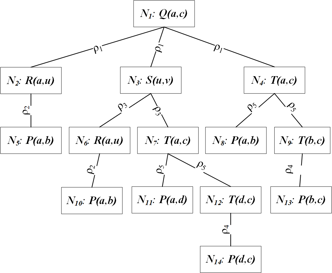
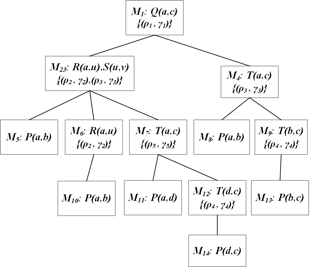
Figure 3: Proof tree (left) and witness (right) for atom $Q(a,c)$ in Examples 4.1 and 5.2.

Example 4.1.

Let $\Pi=\{\rho_{1},\dots,\rho_{5}\}$ be the Datalog^± program with $\rho_{1}\!:\ Q(x,w)\leftarrow R(x,y),$ $S(y,z),T(x,w)$;  $\rho_{2}\!:\ \exists z\leavevmode\nobreak\ R(x,z)\leftarrow P(x,y)$;  $\rho_{3}\!:\ \exists z\leavevmode\nobreak\ S(x,z)\leftarrow R(w,x),T(w,y)$;  $\rho_{4}\!:\ T(x,y)\leftarrow P(x,y)$;  $\rho_{5}\!:\ T(x,y)\leftarrow P(x,z),T(z,y)$. This program belongs to Datalog^±,¬sg, and – although not necessary to build a proof tree for it – we notice that it is also warded: ${\it Aff}(\Pi)=\{R[2],S[2],S[1]\}$; and all other positions are not affected. Rule $\rho_{3}$ is warded with ward $R(w,x)$ (where $x$ is the only dangerous variable in this rule). All other rules are trivially warded because they have no dangerous variables.

Now let $D=\{P(a,b),P(b,c),P(a,d),P(d,c)\}$. A possible proof tree for $Q(a,c)$ is shown in Figure 3 on the left. It is important to note that nodes $N_{2}$ and $N_{6}$ introducing labelled null $u$ are labelled with the same atom and give rise to identical subtrees. Of course, $R(a,u)$ could also result from a chase step applying $\rho_{2}$ to $P(a,d)$. However, this would generate a null different from $u$ and, subsequently, the nulls in $R(a,\_)$ and $S(\_,v)$ (in $N_{2}$ and $N_{3}$) would be different, and rule $\rho_{1}$ could not be applied anymore. In contrast, the nodes $N_{4}$ and $N_{7}$ with label $T(a,c)$ span different subtrees. This is desired: there are two possible derivations for each occurrence of atom $T(a,c)$ in the PT. $\Box$

Here we deviate slightly from the definition of PTs in [4], in that we allow the same ground atom to have different derivations. This is needed to detect duplicates and to make sure that PTs in fact constitute a generalization of the derivation trees in Section 2.1. Moreover, condition (8) is needed to avoid non-isomorphic PTs by “unforced” repetition of nulls (i.e., identical nulls that are not required by a join condition further up in the tree). Analogous to the generalization in Section 2.1 of DTs for Datalog to DTs for Datalog^¬s, it is easy to generalize proof trees to Datalog^±,¬sg. Here it is important that we only allow stratified ground negation. Hence, analogously to DTs for Datalog^¬s, we allow negated ground atoms $\neg A$ to occur as node labels of leaf nodes in a PT, provided that the positive atom $A$ has no PT. Moreover, it is no problem to allow also multiset EDBs since, as in Section 2.1, we can keep duplicates apart by means of a coloring function col.

Finally, we can define proof trees ${\mathcal{T}}$ and ${\mathcal{T}}^{\prime}$ as equivalent, denoted ${\mathcal{T}}\equiv{\mathcal{T}}^{\prime}$, if one is obtained from the other by renaming of nulls. We can thus normalize PTs by assuming that nulls in node labels are from some fixed set $\{u_{1},u_{2}\,\dots\}$ and that these nulls are introduced in the labels of the PT by some fixed-order traversal (e.g., top-down, left-to-right).

For a PT ${\mathcal{T}}$, we define ${\it Atoms}({\mathcal{T}})$ as ${\it col}^{-1}$ of the root when ${\mathcal{T}}$ is a single-node tree, and the root-label of ${\mathcal{T}}$, otherwise. For a set of PTs $\mathfrak{T}$:  ${\it Atoms}(\mathfrak{T}):=\biguplus\{{\it Atoms}({\mathcal{T}})\leavevmode\nobreak\ |\leavevmode\nobreak\ {\mathcal{T}}\in\mathfrak{T}\}$, which is a multiset that multi-contains $D$.  If ${\it PT}(\Pi,$ ${\it col}(D))$ is the set of normalized, non-equivalent PTs, the proof-tree bag (PTB) semantics for $\Pi$ is the multiset ${\it PTBS}(\Pi,D):={\it Atoms}({\it PT}(\Pi,{\it col}(D)))$. For a ground atom $A$, ${\it mult}(A,{\it PTBS}(\Pi,D))$ denotes the multiplicity of $A$ in the multiset ${\it PTBS}(\Pi,D)$.

Example 4.2.

(ex. 4.1 cont.) To compute ${\it PTBS}(\Pi,D)$ for $\Pi$ and $D$ from Example 4.1, we have to determine all proof trees of all ground atoms derivable from $\Pi$ and $D$. In Figure 3, we have already seen one proof tree for $Q(a,c)$; and we have observed that the sub-proof tree of $R(a,u)$ rooted at nodes $N_{2}$ and $N_{6}$ could be replaced by a child node with label $P(a,d)$ (either both subtrees or none has to be changed). In total, the ground atom $Q(a,c)$ has 8 different proof trees wrt. $\Pi$ and $D$ (multiplying the 2 possible derivations of atom $R(a,u)$ with 4 derivations for the two occurrences of the atom $T(a,c)$ in nodes $N_{4}$ and $N_{7}$). The other ground atoms derivable from $\Pi$ and $D$ are $T(a,c)$ (with 2 possible PTs as discussed in Example 4.1) and the atoms $T(i,j)$ for each $P(i,j)$ in $D$. Hence, we have ${\it PTBS}(\Pi,D)=D\cup\{T(a,b),T(b,c),T(a,d),T(d,a),T(a,c),T(a,c),Q(a,c),\dots,Q(a,c)\}$. $\Box$

Clearly, every Datalog^¬s program is a special case of a warded Datalog^±,¬sg program. It is easy to verify that the PTB semantics indeed generalizes the DTB semantics:

Proposition 4.3.

Let $\Pi$ be a Datalog^¬s program and $D$ an EDB (possibly with duplicates). Then ${\it DTBS}(\Pi,D)={\it PTBS}(\Pi,D)$ holds.

4.2 Extension of the PBB Semantics to Datalog^±,¬sg

We now extend also the PBB semantics to Datalog^±,¬sg programs $\Pi$. First, in all predicates of $\Pi$, we add position 0 to carry tid-variables. Then every rule $\rho\in\Pi$ of the form $\rho\!:\ \exists\bar{y}H(\bar{y},\bar{x})\ \leftarrow\ A_{1}(\bar{x}_{1}),A_{2}(\bar{x}_{2}),\ldots,A_{k}(\bar{x}_{k})$, with $k>0,\ \bar{x}\subseteq\cup_{i}\bar{x}_{i}$, becomes the rule  $\rho^{+}\!:\ \exists z\exists\bar{y}\ H(z;\bar{y},\bar{x})\leftarrow A_{1}(z_{1};\bar{x}_{1}),A_{2}(z_{2};\bar{x}_{2}),\ldots,A_{k}(z_{k};\bar{x}_{k})$, with fresh, different variables $z,z_{1},\ldots,z_{k}$. Now consider a rule $\rho\in\Pi$ of the form $\rho\!:\ \exists\bar{y}H(\bar{y}\bar{x})\ \leftarrow\ A_{1}(\bar{x}_{1}),\ldots,A_{k}(\bar{x}_{k}),\neg B_{1}(\bar{x}_{k+1}),\ldots,\neg B_{\ell}(\bar{x}_{k+\ell}),$ with $\bar{x}_{k+1},\ldots,\bar{x}_{k+\ell}\subseteq\bigcup_{i=1}^{k}\bar{x}_{i}$; we transform it into the following two rules:

$$\rho^{\prime}\!:\ \exists z\exists\bar{y}H(z;\bar{y},\bar{x}) \leavevmode\nobreak\ \leftarrow\leavevmode\nobreak\ A_{1}(z_{1};\bar{x}_{1}),\ldots,A_{k}(z_{k};\bar{x}_{k}),\neg{\it Aux}_{1}^{\rho}(\bar{x}_{k+1}),\ldots,\neg{\it Aux}_{\ell}^{\rho}(\bar{x}_{k+\ell}),\leavevmode\nobreak\ \leavevmode\nobreak\ \leavevmode\nobreak\ \leavevmode\nobreak\ \leavevmode\nobreak\$$ (6)

$${\it Aux}_{i}^{\rho}(\bar{x}_{k+i}) \leavevmode\nobreak\ \leftarrow\leavevmode\nobreak\ B_{i}(z_{i};\bar{x}_{k+i}),\ \ i=1,\ldots,\ell.$$

Analogously to Theorem 3.2, the resulting program also belongs to Datalog^±,¬sg. Finally, as in Section 3, the ground atoms in the multiset EDB $D$ are extended in $D^{+}$ by nulls from ${\mathcal{I}}=\{\iota_{1},\iota_{2},\dots\}$ as tids in position 0 to keep apart duplicates. For an instance $I$, we write $I_{\downarrow}$ to denote the set of atoms in $I$ such that all positions except for position 0 (the tid) carry a ground term (from $\mathbf{C}$). Analogously to Definition 3.4, we then define the program-based bag semantics (PBB semantics) of a Datalog^±,¬sg program $\Pi$ and multiset EDB $D$ as ${\it PBBS}(\Pi,D):=\mathcal{DI}({\it Chase}(\Pi^{+},D^{+})_{\downarrow})=\{\!\{P(\bar{a})\leavevmode\nobreak\ |\leavevmode\nobreak\ P(\bar{a})$ is ground and $P(t;\bar{a})\in{\it Chase}(\Pi^{+},D^{+})\}\!\}$. For a ground atom $A$ (here, without nulls or tids), ${\it mult}(A,{\it PBBS}(\Pi,D))$ denotes the multiplicity of $A$ in the multiset ${\it PBBS}(\Pi,D)$.

Example 4.4.

(ex. 4.1 and 4.2 cont.) The transformations of Datalog^±,¬sg program $\Pi$ and multiset EDB $D$ from Example 4.1 are $D^{+}=\{P(\iota_{1},a,b),P(\iota_{2},b,c),P(\iota_{3},a,d),P(\iota_{4},d,c)\}$ and $\Pi^{+}=\{\rho^{+}_{1},\rho^{+}_{2},\rho^{+}_{3},\rho^{+}_{4},\rho^{+}_{5}\}$ with: $\rho_{1}^{+}\!:\ (\exists u)Q(u,x,w)\leftarrow R(v_{1},r,y),S(v_{2},y,z),T(v_{3},x,w)$;  $\rho_{2}^{+}\!:\ (\exists u,z)R(u,x,z)\leftarrow P(v,x,y)$;  $\rho_{3}^{+}\!:\ (\exists u,z)S(u,x,z)$ $\leftarrow R(v_{1},w,x),T(v_{2},w,y)$;  $\rho_{4}^{+}\!:\ (\exists u)T(u,x,y)\leftarrow P(v,x,y)$;  $\rho_{5}^{+}\!:\ (\exists u)T(u,x,y)\leftarrow P(v_{1},x,z),$ $T(v_{2},z,y)$.

Applying program $\Pi^{+}$ to instance $D^{+}$ gives, for example, the following chase sequence for deriving the atoms $T(\iota_{5},d,c),T(\iota_{7},a,c),T(\iota_{8},b,c),Q(\iota_{11},a,c)$, which correspond to the ground atoms in the proof tree in Figure 3, left: $D^{+}\leadsto_{\rho_{4}^{+}}T(\iota_{5},d,c)\leadsto_{\rho_{2}^{+}}R(\iota_{6},a,u)\leadsto_{\rho_{5}^{+}}T(\iota_{7},a,c)\leadsto_{\rho_{4}^{+}}T(\iota_{8},b,c)\leadsto_{\rho_{3}^{+}}S(\iota_{9},u,v)\leadsto_{\rho_{5}^{+}}T(\iota_{10},a,c)\leadsto_{\rho_{1}^{+}}Q(\iota_{11},a,c).$ Implicitly, we thus also turn the PTs rooted at $N_{4}$, $N_{7}$, and $N_{9}$ into chase sequences. In total, we get in ${PBBS}(\Pi,D)$ precisely the atoms and multiplicities as in $PTBS(\Pi,D)$ for Example 4.2. $\Box$

In principle, the above transformation $\Pi^{+}$ and the PBB semantics are applicable to any program $\Pi$ in Datalog^±,¬sg. However, in the first place, we are interested in warded programs $\Pi$. It is easy to verify that wardedness of $\Pi$ carries over to $\Pi^{+}$:

Proposition 4.5.

If $\Pi$ is a warded Datalog^±,¬sg program, then so is $\Pi^{+}$.

Proof 4.6 (Proof Idea).

The key observation is that the only additional affected positions in $\Pi^{+}$ are the tids at position 0. However, the variables at these positions occur only once in each rule and are never propagated from the body to the head. Hence, they do not destroy wardedness.

We conclude this section with the analogous result of Theorem 3.5:

Theorem 4.7.

For ground atoms $A$, ${\it mult}(A,{\it PTBS}(\Pi,D))={\it mult}(A,{\it PBBS}(\Pi,D))$. Hence, for a warded Datalog^±,¬sg program $\Pi$ and multiset EDB $D$,  ${\it PTBS}(\Pi,D)={\it PBBS}(\Pi,D)$.

5 Decidability and Complexity of Multiplicity

For Datalog^¬s programs, the following problems related to duplicates have been investigated:

• FFE:  Given a program $\Pi$, a database $D$, and a predicate $P$, decide if every derivable ground $P$-atom has a finite number of DTs.

• FEE:  Given a program $\Pi$ and a predicate $P$, decide if every derivable ground $P$-atom has a finite number of DTs for every database $D$.

It has been shown in [22] that FFE is decidable (even in PTIME data complexity), whereas FEE is undecidable. We extend this study by considering warded Datalog^±,¬sg instead of Datalog^¬s, and by computing the concrete multiplicities in case of finiteness. We thus study the following problems:

• FINITENESS: For fixed warded Datalog^±,¬sg program $\Pi$:  Given a multiset database $D$ and a ground atom $A$, does $A$ have finite multiplicity, i.e., is ${\it mult}(A,{\it PBBS}(\Pi,D))$ finite?

• MULTIPLICITY: For fixed warded Datalog^±,¬sg program $\Pi$:  Given a multiset database $D$ and a ground atom $A$, compute the multiplicity of $A$, i.e. ${\it mult}(A,{\it PBBS}(\Pi,D))$.

We will show that both problems defined above can be solved in polynomial time (data complexity). In case of the FINITENESS problem, we thus generalize the result of [22] for the FFE problem from Datalog^¬s to Datalog^±,¬sg. In case of the MULTIPLICITY problem, no analogous result for Datalog or Datalog^¬s has existed before. The following example illustrates that, even if $\Pi$ is a Datalog program with a single rule, we may have exponential multiplicities. Hence, simply computing all DTs or (in case of Datalog^±) all PTs is not a viable option if we aim at polynomial time complexity.

Example 5.1.

Let $D=\{E(a_{0},a_{1}),E_{(}a_{1},a_{2}),\dots,E(a_{n-1},a_{n})\}\cup\{P(a_{0},a_{1}),C(b_{0}),C(b_{1})\}$ for $n\geq 1$ and let $\Pi=\{\rho\}$ with $\rho\!:P(x,y)\leftarrow P(x,z),E(z,y),C(w)$. Intuitively, $E$ can be considered as an edge relation and $P$ is the corresponding path relation for paths starting at $a_{0}$. The $C$-atom in the rule body (together with the two $C$-atoms in $D$) has the effect that there are always 2 possible derivations to extend a path. It can be verified by induction over $i$, that atom $P(a_{0},a_{i})$ has $2^{i-1}$ possible derivations from $D$ via $\Pi$. In particular, $P(a_{0},a_{n})$ has multiplicity $2^{n-1}$.

Note that, if we add atom $E(a_{1},a_{1})$ to $D$ (i.e., a self-loop, so to speak), then every atom $P(a_{0},a_{i})$ with $i\geq 1$ has infinite multiplicity. Intuitively, the infinitely many different derivation trees correspond to the arbitrary number of cycles through the self-loop $E(a_{1},a_{1})$ for a path from $a_{0}$ to $a_{i}$. $\Box$

Our PTIME-membership results will be obtained by appropriately adapting the tractability proof of CQA for warded Datalog^± in [4], which is based on the algorithm ProofTree for deciding if $D\cup\Pi\models P(\bar{c})$ holds for database $D$, warded Datalog^± program $\Pi$, and ground atom $P(\bar{c})$. That algorithm works in ALOGSPACE (data complexity), i.e., alternating logspace, which coincides with PTIME [12]. It assumes $\Pi$ to be normalized in such a way that each rule in $\Pi$ is either head-grounded (i.e., each term in the head is a constant or a harmless variable) or semi-body-grounded (i.e., there exists at most one body atom with harmful variables). Algorithm ProofTree starts with ground atom $P(\bar{c})$ and applies resolution steps until the database $D$ is reached. It thus proceeds as follows:

• If $P(\bar{c})\in D$, then accept. Otherwise, guess a head-grounded rule $\rho\in\Pi$ whose head can be matched to $P(\bar{c})$ (denoted as $\rho\rhd P(\bar{c})$). Guess an instantiation $\gamma$ on the variables in the body of $\rho$ so that $\gamma({\it head}(\rho))=P(\bar{c})$. Let ${\mathcal{S}}=\gamma({\it body}(\rho))$.

• Partition ${\mathcal{S}}$ into $\{{\mathcal{S}}_{1},\dots,{\mathcal{S}}_{n}\}$, such that each null occurring in ${\mathcal{S}}$ occurs in exactly one ${\mathcal{S}}_{i}$, and each set ${\mathcal{S}}_{i}$ is chosen subset-minimal with this property. The purpose of these sets ${\mathcal{S}}_{i}$ of atoms is to keep together, in the parallel universal computations of ProofTree, the nulls in ${\mathcal{S}}$ until the atom in which they are created is known.

• Universally select each set ${\mathcal{S}}^{\prime}\in\{{\mathcal{S}}_{1},\dots,{\mathcal{S}}_{n}\}$ and “prove” it: If ${\mathcal{S}}^{\prime}$ consists of a single ground atom $P^{\prime}(\bar{c}^{\prime})$, then call ProofTree recursively for $D$, $\Pi$, $P^{\prime}(\bar{c}^{\prime})$. Otherwise, do the following:

  (1) For each atom $A\in{\mathcal{S}}^{\prime}$, guess rule $\rho_{A}$ with $\rho_{A}\rhd A$ and guess variable instantiation $\gamma_{A}$ on the variables in the body of $\rho_{A}$ such that $A=\gamma_{A}({\it head}(\rho_{A}))$.

  (2) The set $\bigcup_{A\in{\mathcal{S}}^{\prime}}\gamma_{A}({\it body}(\rho_{A}))$ is partitioned as above and each component of this partition is proved in a parallel universal computation.

The key to the ALOGSPACE complexity of algorithm ProofTree is that the data structure propagated by this algorithm fits into logarithmic space. This data structure is given by a pair $({\mathcal{S}},{{\mathcal{R}}}_{{\mathcal{S}}})$, where ${\mathcal{S}}$ is a set of atoms (such that $|{\mathcal{S}}|$ is bounded by the maximum number of body atoms of the rules in $\Pi$) and ${{\mathcal{R}}}_{{\mathcal{S}}}$ is a set of pairs $(z,x)$, where $z$ is a null occurring in ${\mathcal{S}}$ and $x$ is either an atom $A$ (meaning that null $z$ was created when the application of some rule $\rho$ generated the atom $A$ containing this null $z$) or the symbol $\varepsilon$ (meaning that we have not yet found such an atom $A$). A witness for a successful computation of ProofTree is then given by a tree with existential and universal nodes, with an existential node $N$ consisting of a pair $({\mathcal{S}},{{\mathcal{R}}}_{{\mathcal{S}}})$; a universal node $N$ indicates the guessed rule $\rho_{A}$ together with the instantiation $\gamma_{A}$ for each atom $A\in{\mathcal{S}}$ at the (existential) parent node of $N$. The child nodes of each universal node $N$ are obtained by partitioning $\bigcup_{A\in{\mathcal{S}}}\gamma_{A}({\it body}(A))$ as described above and computing the corresponding set ${{\mathcal{R}}}_{{\mathcal{S}}}$. At the root, we thus have an existential node labelled $({\mathcal{S}},{{\mathcal{R}}}_{{\mathcal{S}}})=(\{P(\bar{c})\},\emptyset)$. Each leaf node is a universal node labelled with $(B,\emptyset)$ for some ground atom $B\in D$. Hence, such a node corresponds to an accept-state.

Example 5.2.

Recall $\Pi$ and $D$ from Example 4.1. A proof tree of ground atom $Q(a,c)$ is shown in Figure 3 on the left. On the right, we display the witness of the corresponding successful computation of ProofTree. Note that witnesses have a strict alternation of existential and universal nodes. In the witness in Figure 3, we have merged each existential node and its unique universal child node to make the correspondence between a PT and a witness yet more visible. In particular, on each depth level of the trees, we have exactly the same set of atoms (with the only difference, that in the witness these atoms are grouped together to sets ${\mathcal{S}}$ by null-occurrences). In this simple example, only node $M_{23}$ contains such a group of atoms, namely the atoms from the nodes $N_{2}$ and $N_{3}$ in the PT.

In order not to overburden the figure, we have left out the sets ${{\mathcal{R}}}_{{\mathcal{S}}}$ carrying the information on the introduction of nulls. In this simple example, the only node with a non-empty set ${{\mathcal{R}}}_{{\mathcal{S}}}$ is $M_{6}$, with ${{\mathcal{R}}}_{{\mathcal{S}}}=\{(u,R(a,u)\}$, i.e. we have to pass on the information that the null $u$ in node $M_{23}$ was introduced by applying some rule (namely $\rho_{2}$) which generated the atom $R(a,u)$. We thus ensure (when proceeding from node $M_{6}$ to node $M_{10}$) that null $u$ is introduced in the same way as before.

The information from the universal node below each existential node is displayed in the second line of each node: here we have pairs consisting of the guessed rule $\rho$ plus the guessed instantiation $\gamma$ for each atom in the corresponding set ${\mathcal{S}}$ (as mentioned above, ${\mathcal{S}}$ is a singleton in all nodes except for $M_{23}$). For instance, $\gamma_{1}$ in node $M_{1}$ denotes the substitution $\gamma_{1}=\{x\leftarrow a,y\leftarrow u,z\leftarrow v,w\leftarrow c\}$. Only in node $M_{23}$, we have 2 pairs $(\rho_{2},\gamma_{2}),(\rho_{3},\gamma_{3})$ with $\gamma_{2}=\{x\leftarrow a,y\leftarrow b\}$ and $\gamma_{3}=\{w\leftarrow a,x\leftarrow u,y\leftarrow c\}$. Note that the subscripts $i$ of the $\gamma_{i}$’s in Figure 3 are to be understood local to the node. For instance, the two different applications of rule $\rho_{4}$ in nodes $M_{9}$ and $M_{12}$ are with the instantiations $\gamma_{4}=\{x\leftarrow b,y\leftarrow c\}$ (in $M_{9}$) and $\gamma_{4}=\{x\leftarrow d,y\leftarrow c\}$ (in $M_{12}$), respectively. $\Box$

The above example illustrates the close relationship between PTs ${\mathcal{T}}$ and witnesses ${\mathcal{W}}$ of the ProofTree algorithm. However, our goal is a one-to-one correspondence, which requires further measures: for witness trees, we thus assume from now on (as in Example 5.2) that each existential node is merged with its unique universal child node and that nulls are renamed apart: that is, whenever nulls are introduced by a resolution step of ProofTree, then all nulls in ${\it nulls}(\gamma({\it body}(\rho)))\setminus{\it nulls}(\gamma({\it head}(\rho)))$ must be fresh (that is, they must not occur elsewhere in ${\mathcal{W}}$). Moreover, we eliminate redundant information from PTs and witnesses by pruning repeated subtrees: let $N$ be a node in a PT ${\mathcal{T}}$ such that some null is introduced via atom $A$ in $\lambda(N)$, and let $N$ be closest to the root with this property, then prune all other subtrees below all nodes $M\neq N$ with $\lambda(M)=A$. Likewise, if a node in a witness ${\mathcal{W}}$ contains an atom $A$ and the pair $(z,A)$ in ${{\mathcal{R}}}_{{\mathcal{S}}}$, then we omit the resolution step for $A$. We refer to the reduced PT of ${\mathcal{T}}$ as ${\mathcal{T}}^{*}$ and to the reduced witness of ${\mathcal{W}}$ as ${\mathcal{W}}^{*}$. For instance, in the PT in Figure 3, we delete the node $N_{10}$ because the information on how to derive atom $R(a,u)$ is already contained in the subtree rooted at node $N_{2}$. Likewise, in the witness in Figure 3, we omit the resolution step for atom $R(a,u)$ in node $M_{6}$, because, in this node, we have ${{\mathcal{R}}}_{{\mathcal{S}}}=\{(u,R(a,u)\}$. Hence, it is known from some resolution step “above” that $u$ must be introduced via this atom and its derivation is checked elsewhere. We thus delete $M_{10}$.

It is straightforward to construct a reduced witness ${\mathcal{W}}^{*}$ from a given reduced PT ${\mathcal{T}}^{*}$, and vice versa. We refer to these constructions as ${\mathcal{T}}2{\mathcal{W}}$ and ${\mathcal{W}}2{\mathcal{T}}$, respectively: Given ${\mathcal{T}}^{*}$, we obtain ${\mathcal{W}}^{*}$ by a top-down traversal of ${\mathcal{T}}^{*}$ and merging siblings if they share a null. Moreover, if the label at a child node in ${\mathcal{T}}^{*}$ was created by applying rule $\rho$ with substitution $\gamma$, then we add $(\rho,\gamma)$ to the node label in ${\mathcal{W}}^{*}$. Finally, if such a rule application generates a new null $z$, then we add $(z,\gamma({\it head}(\rho))$ to ${{\mathcal{R}}}_{{\mathcal{S}}}$ of every child node which still contains null $z$. Conversely, we obtain ${\mathcal{T}}^{*}$ from a reduced witness ${\mathcal{W}}^{*}$ by a bottom-up traversal of ${\mathcal{W}}^{*}$, where we turn every node labelled with $k$ atoms into $k$ siblings, each labelled with one of these atoms. The edge labels $\rho$ in ${\mathcal{T}}^{*}$ are obtained from the corresponding $(\rho,\gamma)$ labels in the node in ${\mathcal{W}}^{*}$. In summary, we have:

Lemma 5.3.

There is a one-to-one correspondence between reduced proof trees ${\mathcal{T}}^{*}$ for a ground atom $P(\bar{c})$ and reduced witnesses ${\mathcal{W}}^{*}$ for its successful ProofTree computations. More precisely, given ${\mathcal{T}}^{*}$, we get a reduced witness as ${\mathcal{T}}2{\mathcal{W}}({\mathcal{T}}^{*})$; given ${\mathcal{W}}^{*}$, we get a reduced PT as ${\mathcal{W}}2{\mathcal{T}}({\mathcal{W}}^{*})$ with ${\mathcal{W}}2{\mathcal{T}}({\mathcal{T}}2{\mathcal{W}}({\mathcal{T}}^{*}))={\mathcal{T}}^{*}$ and ${\mathcal{T}}2{\mathcal{W}}({\mathcal{W}}2{\mathcal{T}}({\mathcal{W}}^{*}))={\mathcal{W}}^{*}$. $\Box$

So far, we have only considered warded Datalog^±, without negation. However, this restriction is inessential. Indeed, by the definition of warded Datalog^±,¬sg, negated atoms can never contain a null in the chase. Hence, one can easily get rid of negation (in polynomial time data complexity) by computing for one stratum after the other the answer $Q(\Pi,D)$ to query $Q$ with $Q\equiv P(x_{1},\dots,x_{n})$, i.e., all ground atoms $P(a_{1},\dots,a_{n})$ with $\Pi\cup D\models P(a_{1},\dots,a_{n})$. We can then replace all occurrences of $\neg P(t_{1},\dots,t_{n})$ in any rule of $\Pi$ by the positive atom $P^{\prime}(t_{1},\dots,t_{n})$ (for a new predicate symbol $P^{\prime}$) and add to the instance all ground atoms $P^{\prime}(a_{1},\dots,a_{n})$ with $(a_{1},\dots,a_{n})\not\in Q(D,\Pi)$. Hence, all our results proved in this section for warded Datalog^± also hold for warded Datalog^±,¬sg.

Clearly, there is a one-to-one correspondence between proof trees PT ${\mathcal{T}}$ and their reduced forms ${\mathcal{T}}^{*}$. Hence, together with Lemma 5.3, we can compute the multiplicities by computing (reduced) witness trees. This allows us to obtain the results below:

Theorem 5.4.

Let $\Pi$ be a warded Datalog^±,¬sg program and $D$ a database (possibly with duplicates). Then there exists a bound $K$ which is polynomial in $D$, s.t. for every ground atom $A$:

1. $A$ has finite multiplicity if and only if all reduced witness trees of $A$ have depth $\leq K$.

2. If $A$ has infinite multiplicity, then there exists at least one reduced witness tree of $A$ whose depth is in $[K+1,2K]$.

Proof 5.5 (Proof Idea).

Recall that the data structure propagated by the ProofTree algorithm consists of pairs $({\mathcal{S}},{{\mathcal{R}}}_{{\mathcal{S}}})$. We call pairs $({\mathcal{S}},{{\mathcal{R}}}_{{\mathcal{S}}})$ and $({\mathcal{S}}^{\prime},{\mathcal{R}}_{{\mathcal{S}}^{\prime}})$ equivalent if one can be obtained from the other by renaming of nulls. The bound $K$ corresponds to the maximum number of non-equivalent pairs $({\mathcal{S}},{{\mathcal{R}}}_{{\mathcal{S}}})$ over the given signature and domain of $D$. By the logspace bound on this data structure, there can only be polynomially many (w.r.t. $D$) such pairs. For the first claim of the theorem, suppose that a (reduced) witness tree ${\mathcal{W}}^{*}$ has depth greater than $K$; then there must be a branch with two nodes $N$ and $N^{\prime}$ with equivalent pairs $({\mathcal{S}},{{\mathcal{R}}}_{{\mathcal{S}}})$ and $({\mathcal{S}}^{\prime},{\mathcal{R}}_{{\mathcal{S}}^{\prime}})$. We get infinitely many witness trees by arbitrarily often iterating the path between $N$ and $N^{\prime}$.

In principle, Theorem 5.4 suffices to prove decidability of FINITENESS and design an algorithm for the MULTIPLICITY: just chase database $D$ with the transformed warded Datalog program $\Pi^{+}$ up to depth $2K$. If the desired ground atom $A$ extended by some tid is generated at a depth greater than $K$, then conclude that $A$ has infinite multiplicity. Otherwise, the multiplicity of $A$ is equal to the number of atoms of the form $(\iota;A)$ in the chase result. However, this chase of depth $2K$ may produce an exponential number of atoms and hence take exponential time. Below we show that we can in fact do significantly better:

Theorem 5.6.

For warded Datalog^±,¬sg programs, both the FINITENESS problem and the MULTIPLICITY problem can be solved in polynomial time.

Proof 5.7 (Proof Idea).

A decision procedure for the FINITENESS problem can be obtained by modifying the ALOGSPACE algorithm ProofTree from [4] in such a way that we additionally “guess” a branch in the witness tree with equivalent labels. The additional information thus needed also fits into logspace.

The MULTIPLICITY problem can be solved in polynomial time by a tabling approach to the ProofTree algorithm. We thus store for each (non-equivalent) value of $(S,R_{S})$ how many (reduced) witness trees it has and propagate this information upwards for each resolution step encoded in the (reduced) witness tree.

6 Multiset Relational Algebra (MRA)

Following [20, 21], we consider multisets (or bags) $M$ and elements $e$ (from some domain) with non-negative integer multiplicities, ${\it mult}(e,M)$ (recall from Section 2.1 that, by definition, $e\in M$ iff ${\it mult}(e,M)\geq 1$). Now consider multiset relations $R,S$. Unless stated otherwise, we assume that $R,S$ contain tuples of the same arity, say $n$. We define the following multiset operations of MRA: the multiset union, $\uplus$, is defined by $R\uplus S:=T$, with ${\it mult}(e,T):={\it mult}(e,R)+{\it mult}(e,S)$. Multiset selection, $\sigma^{\it m}_{C}(R)$, with a condition $C$, is defined as the multiset $T$ containing all tuples in $R$ that satisfy $C$ with the same multiplicities as in $R$. For multiset projection $\pi^{\it m}_{\bar{k}}(R)$, we get the multiplicities ${\it mult}(e,\pi^{\it m}_{\bar{k}}(R))$ by summing up the multiplicities of all tuples in $R$ that, when projected to the positions $\bar{k}=\langle i_{1},\ldots,i_{k}\rangle$, produce $e$. For the multiset (natural) join ${R\Join^{\!{\it m}}\!S}$, the multiplicity of each tuple $t$ is obtained as the product of multiplicities of tuples from $R$ and of tuples from $S$ that join to $t$.

For the multiset difference, two definitions are conceivable:  Majority-based, or “monus" difference (see e.g. [15]), given by  $R\ominus S:=T$, with ${\it mult}(e,T):={\it max}\{{\it mult}(e,R)-{\it mult}(e,S),0\}$. There is also the “all-or-nothing" difference:  $R\otimes S:=T$, with ${\it mult}(e,T):={\it mult}(e,R)\mbox{ if }$ $e\notin S$ and ${\it mult}(e,T):=0$, otherwise. Following [22], we have only considered $\otimes$ so far (implicitly, starting with Datalog^¬s, in Section 2.1). The multiset intersection $\cap_{m}$ is not treated or used in any of [2, 20, 21, 22]. Extending the DTB semantics from [21] to $\cap_{m}$ would treat it as a special case of the join, which may be counter-intuitive, e.g., $\{a,a,b\}\cap_{\it m}\{a,a,a,c\}:=\{a,a,a,a,a,a\}$. Alternatively, we could define “minority-based" intersection $R\cap_{\it mb}S$, which returns each element with its minimum multiplicity, e.g., $\{a,a,b\}\cap_{\it mb}\{a,a,a,c\}:=\{a,a\}$.

We consider MRA with the following basic multiset operations: multiset union $\uplus$, multiset projection $\pi^{\it m}_{\bar{k}}$, multiset selection $\sigma^{\it m}_{C}$, with $C$ a condition, multiset (natural) join $\Join^{\!{\it m}}$, and (all-or-nothing) multiset difference $\otimes$. We can also include duplicate elimination in MRA, which becomes operation $\mathcal{DI}$ of Definition 3.3 when using tids. Being just a projection in the latter case, it can be represented in Datalog. For the moment, we consider multiset-intersection as a special case of multiset (natural) join $\Join^{\!{\it m}}$. It is well known that the basic, set-oriented relational algebra operations can all be captured by means of (non-recursive) Datalog^¬s programs (cf. [1]). Likewise, one can capture MRA by means of (non-recursive) Datalog^¬s programs with multiset semantics (see e.g. [2]). Together with our transformation into set semantics of Datalog^±,¬sg, we thus obtain:

Theorem 6.1.

The Multiset Relational Algebra (MRA) can be represented by warded Datalog^±,¬sg with set semantics. $\Box$

As a consequence, the MRA operations can still be performed in polynomial-time (data complexity) via Datalog^±,¬sg. This result tells us that MRA – applied at the level of an EDB with duplicates – can be represented in warded Datalog, and uniformly integrated under the same logical semantics with an ontology represented in warded Datalog.

We now retake multiset-intersection (and later also multiset-difference), which appears as  $\cap_{m}$ and $\cap_{\it mb}$. The former does not offer any problem for our representation in Datalog^± as above, because it is a special case of multiset join. In contrast, the minority-based intersection, $\cap_{\it mb}$, is more problematic. First, the DTB semantics does not give an account of it in terms of Datalog that we can use to build upon. Secondly, our Datalog^±-based formulation of duplicate management with MRA operations is set-theoretic. Accordingly, to investigate the representation of the bag-based operation $\cap_{\it mb}$ by means of the latter, we have to agree on a set-based reformulation $\cap_{\it mb}$. We propose for it a tid-based (set) representation, because tid creation becomes crucial to make it a deterministic operation. Accordingly, for multi-relations $P$ and $R$ with the same arity $n$ (plus $1$ for tids), we define:

$$P\cap_{\it mb}Q:=\{(i;\bar{a})\ |\ (i;\bar{a})\in\left\{\begin{array}[]{ll}P&\mbox{ if }|\pi_{0}(\sigma_{1..n=\bar{a}}(P))|\leq|\pi_{0}(\sigma_{1..n=\bar{a}}(Q))|\\ Q&\mbox{ otherwise}\end{array}\right.\}.$$ (7)

Here, we only assume that tids are local to a predicate, i.e. they act as values for a surrogate key. Intuitively, we keep for each tuple in the result the duplicates that appear in the relation that contains the minimum number of them. Here, $\pi_{0}$ denotes the projection on the $0$-th attribute (for tids), and $\sigma_{1..n=\bar{a}}$ is the selection of those tuples which coincide with $\bar{a}$ on the next $n$ attributes. This operation may be non-commutative when equality holds in the first case of (7) (e.g. $\{\langle 1;a\rangle\}\cap_{\it mb}\{\langle 2;a\rangle\}=\{\langle 1;a\rangle\}\neq\{\langle 2;a\rangle\}=\{\langle 2;a\rangle\}\cap_{\it mb}\{\langle 1;a\rangle\}$). Most importantly, it is non-monotonic: if any of the extensions of $P$ or $Q$ grows, the result may not contain the previous result, e.g. $\{\langle 1;a\rangle\}\cap_{\it mb}\{\langle 2;a\rangle\}=\{\langle 1;a\rangle\}\not\supseteq\{\langle 2;a\rangle\}=(\{\langle 1;a\rangle\}\cup\{\langle 3;a\rangle\})\cap_{\it mb}\{\langle 2;a\rangle\}$.  (It is still non-monotonic under the DTB semantics.) We get the following inexpressibility results:

Proposition 6.2.

The minority-based intersection with duplicates $\cap_{\it mb}$ as in (7) cannot be represented in Datalog, (positive) Datalog^±, or FO predicate logic (FOL). The same applies to the majority-based (monus) difference, $\ominus$.

Proof 6.3 (Proof Idea).

By the non-monotonicity of $\cap_{\it mb}$, it is clear for Datalog and (positive) Datalog^±. For the inexpressibility in FOL, the key idea is that with the help of $\cap_{\it mb}$ or $\ominus$ we could express the majority quantifier, which is known to be undefinable in FOL [24, 25].

Proposition 6.4.

The minority-based intersection with duplicates $\cap_{\it mb}$ as in (7) cannot be represented in Datalog^¬s. The same applies to the majority-based difference, $\ominus$.

Proof 6.5 (Proof Idea).

It can be shown that if a logic is powerful enough to express any of $\cap_{\it mb}$ or $\ominus$, then we could express in this logic – for sets $A$ and $B$ – that $|A|=|B\smallsetminus A|$ holds. However, the latter property cannot even be expressed in the logic $L^{\omega}_{\infty\omega}$ under finite structures [13, sec. 8.4.2] and this logic extends Datalog^¬s.

Among future work, we plan to investigate further inexpressibility issues such as, for instance, whether Datalog^±,¬sg is expressive enough to capture $\cap_{\it mb}$ and $\ominus$. More generally, the development of tools to address (in)expressibility results in Datalog^±, with or without negation, is a matter of future research.

7 Conclusions and Future Work

We have proposed the specification of the bag semantics of Datalog in terms of warded Datalog^± with set semantics and we have extended this specification to Datalog^¬s as well as warded Datalog^± and Datalog^±,¬sg. That is, the bag semantics of all these languages can be captured by warded Datalog^±,¬sg with set semantics. We have also discussed Multiset Relational Algebra (MRA) as an immediate application of our results.

Our work underlines that warded Datalog^± is indeed a well-chosen fragment of Datalog^±: it provides a mild extension of Datalog by the restricted use of existentially quantified variables in the rule heads, which suffices to capture certain forms of ontological reasoning [3, 17] and, as we have seen here, the bag semantics of Datalog. At the same time, it maintains favorable properties of Datalog, such as polynomial-time query answering. Actually, the techniques developed for establishing this polynomial-time complexity result for warded Datalog^± in [3, 4] have also greatly helped us to prove our polynomial-time results for the FINITENESS and MULTIPLICTY problems.

Another advantage of warded Datalog^± is the existence of an efficient implementation in the VADALOG system [6]. Further extensions of this system – above all the support of SPARQL with bag semantics based on the Datalog rewriting proposed in [2, 23] – are currently under way. Recall that warded Datalog^±,¬sg was shown to capture a core fragment of SPARQL under OWL 2 QL entailment regimes [16], with set semantics though [3, 17]. Our transformation via warded Datalog^±,¬sg will allow us to capture also the bag semantics.

We are currently also working on further inexpressibility results. Recall that our translation into Datalog^±,¬sg does not cover multiset intersection; moreover, multiset difference is only handled in the all-or-nothing form $\otimes$, while the sometimes more natural form $\ominus$ has been left out (but the former is good enough for application to SPARQL). We conjecture that the two operations $\cap_{\it mb}$ and $\ominus$ are not expressible in Datalog^±,¬sg with set semantics. The verification of this conjecture is a matter of ongoing work.

Finally, we plan to extend our treatment Datalog^±,¬sg with bag semantics. Recall that in Section 4, we have only defined multiplicities for ground atoms (without nulls). With our methods developed here, we can also compute for a non-ground atom $p(u,a)$ (more precisely, with $u$ a null in $\mathbf{B}$) how often it is derived from $D$ via $\Pi$. However, answering questions like “for how many different null values $u$ can $p(u,a)$ be derived?” requires new methods.

Appendix A Proofs for Section 3

Proof A.1 (Proof of Theorem 3.2).

It is easy to verify that, in every $\rho^{+}\in\Pi^{+}$, the only harmful position is the position 0 (i.e, the tid) of each predicate from $\Pi$. However, the variables occurring in position 0 in the rule bodies do not occur in the head. Hence, none of the rules in $\Pi^{+}$ contains a dangerous variable and, therefore, $\Pi^{+}$ is trivially warded. By the same consideration, the auxiliary predicates introduced in (5) above contain only non-affected positions. Since these are the only negated atoms in rules of $\Pi^{+}$, we have only ground negation in $\Pi^{+}$. Finally, the stratification of $\Pi$ carries over to $\Pi^{+}$, where an auxiliary predicate ${\it Aux}_{i}^{\rho}$ introduced for a negated predicate $B_{i}$ in the definition of predicate $H$ by $\rho$ in $\Pi$ ends up in stratum $s$ of $\Pi^{+}$ iff $B_{i}$ is in stratum $s$ in $\Pi$ (cf. (4) and (5)).

Proof A.2 (Proof of Theorem 3.5).

We first consider the case of a Datalog program $\Pi$ (i.e., without negation). It suffices to prove the following claim: for a Datalog program $\Pi$ with multiset EDB $D$, there is a one-to-one correspondence between DTs in ${\it DT}(\Pi,{\it col}(D))$ with root atoms $P(\bar{c})$ and minimal chase-sequences with $\Pi^{+}$ that start with $D^{+}$ and end in atoms $P(\iota;\bar{c})$, with $\iota\in\mathcal{I}$, i.e. that establish $D^{+}\leadsto^{*}P(\iota;\bar{c})$. By “minimality” of a chase-sequence we mean that every intermediate atom derived is used to enforce some rule later along the same sequence.  More precisely: (a)   ${\delta\!:\ {\it col}^{-1}({\it DTBS}(\Pi,D))\cong{\it col}^{-1}({\it Chase}(\Pi^{+},D^{+}))}$, i.e. there are isomorphic as sets. (b)  For every element $e$ (in the data domain):  ${\it mult}(e,{\it col}^{-1}({\it DTBS}(\Pi,D)))={\it mult}(e,$ ${\it Chase}(\Pi^{+},D^{+}))$.

One direction is by induction on the depth of the trees (the other direction is similar, and by induction of the length of the chase sequences). The correspondence is clear for depth 1. Now assume that, for every DT of depth at most $n$, with some root $Q(\bar{c})$, there is exactly one chase sequence ending in $Q(\iota;\bar{c})$.

We now consider trees of depth $n+1$. Let $P(\bar{c})$ be an atom at the root of a DT ${\mathcal{T}}$ obtained from the ground instantiation $\rho_{g}\!:\ P(\bar{c})\leftarrow Q_{1}(\bar{c}_{1}),\ldots,$ $Q_{k}(\bar{c}_{k})$ of a rule $\rho\!:\ P(\bar{x})\leftarrow Q_{1}(\bar{x}_{1}),\ldots,Q_{k}(\bar{x}_{k})$. Then it has distinct children $Q_{1}(\bar{c}_{1}),\ldots,Q_{k}(\bar{c}_{k})$, in this order from left ro right, each of them with a DT ${\mathcal{T}}_{1},\ldots,{\mathcal{T}}_{k}$ of depth at most $n$. These DTs in their turn correspond to distinct chase sequences, $s_{1},\ldots,s_{k}$, starting in $D^{+}$ and with end atom of the form $Q_{1}(\iota_{1}^{\prime};\bar{c}_{1}),\ldots,Q_{1}(\iota_{k}^{\prime};\bar{c}_{k})$, with different $\iota_{j}^{\prime}$s. Then, the interleaved combination of these chase-sequences – to respect the canonical order of rule applications and body atoms – and concatenated suffix “$\leadsto_{\rho_{g}^{+}}\!P(\iota;\bar{c})$"  is exactly the one deriving $P(\iota;\bar{c})$.

It remains to consider the case of a Datalog^¬s program $\Pi$. In this case, we have to consider a chase procedure for Datalog^±,¬s applied to $\Pi^{+}$, and its correspondence to DTs for $\Pi$. The chase for Datalog^±,¬s [10] is similar to that for Datalog^±, except that now it is defined in a stratified manner: If, in the course of a chase sequence the positive part ${\it body}^{+}$ of a Datalog^±,¬s rule with body ${\it body}^{+},{\it body}^{-}$ becomes applicable, the rule is applied as long as the instantiated atoms in ${\it body}^{-}$ have not been generated already, at a previous stratum of the chase (see [10, sec. 10] for details). This has exactly the same effect as the use of negation-as-failure with stratified Datalog^¬s, as can be easily proved by induction of the strata.

Proof A.3 (Proof of Corollary 3.7).

We first consider the case of a Datalog program $\Pi$ (i.e., without negation). Let $M$ be the minimal model of $\Pi\cup\mathcal{SP}(D)$. Then, $\mathcal{SP}({\it Chase}(\Pi^{+},D^{+}))$ $\subseteq M$. This can be seen as follows: every atom $A$ in the former has at least one chase-derivation with $\Pi^{+}\cup D^{+}$, and then, as in the proof of Theorem 3.5, a DT with $\Pi\cup{\it col}(D)$, which is also a derivation tree from $\Pi\cup\cal{SP}(D)$. By the correspondence between top-down and bottom-up evaluations for Datalog, $A\in M$. The other direction is similar.

For a Datalog^¬s program $\Pi$, we use the correspondence between the stratified chase-sequences with $\Pi^{+}\cup D^{+}$ and the stratified, bottom-up computation of the standard model for $\Pi\cup\mathcal{SP}(D)$, as shown in the proof of Theorem 3.5.

Appendix B Proofs for Section 4

Proof B.1 (Proof of Proposition 4.3).

Due to the satisfaction by a Datalog^¬s program of conditions (1)-(4) on proof trees at the beginning of this section (conditions (5)-(8) do not apply to such a program), every PT for an atom $A$ from multiset $D$ and a Datalog^¬s program $\Pi$ $D$ is also a DT for the atom, and the other way around.

Proof B.2 (Proof of Proposition 4.5).

Through the transformation of rules of $\Pi$ into rules of $\Pi^{+}$, the non-zero positions in $\Pi^{+}$ coincide with those in $\Pi$. Hence, ${\it Aff}(\Pi)={\it Aff}(\Pi^{+})\smallsetminus\{P[0]\leavevmode\nobreak\ |\leavevmode\nobreak\ P$ appears in a rule head$\}$ holds. Then, ${\it NonAff}(\Pi^{+})={\it NonAff}(\Pi)\cup\{P[0]\leavevmode\nobreak\ |\leavevmode\nobreak\ P$ does not appear in a rule head$\}$; and, furthermore, ${\it Harmless}(\rho^{+})={\it Harmless}(\rho)\cup\{z_{i}\leavevmode\nobreak\ |\leavevmode\nobreak\ A_{i}$ does not appear in a rule head$\}$. Since tid-variables in bodies do not appear in heads, ${\it Dang}(\rho^{+})={\it Dang}(\rho)$ holds. Thus, for each rule $\rho^{+}$, the variables in ${\it Dang}(\rho^{+})$ already have a ward in $\rho$.

Proof B.3 (Proof of Theorem 4.7).

It suffices to prove that there is a one-to-one correspondence between normalized, non-equivalent PTs in ${\it PT}(\Pi,{\it col}(D))$ with root atoms $P(\bar{c})$ and (minimal) chase-sequences with $\Pi^{+}$ that start with $D^{+}$ and end in atoms $P(\iota;\bar{c})$, with $\iota\in\mathcal{I}$. One direction of the correspondence is is obtained by induction on the depth of PTs (the other one is similar, by induction on the length of chase sequences). The assumptions on canonical orders of application of rules and generation of PTs are crucial.

The correspondence is clear for PT depth 1. Now assume that, for every PT of depth at most $n$, with some root $Q(\bar{c})$, there is exactly one chase sequence ending in $Q(\iota;\bar{c})$.  We now consider a PT ${\mathcal{T}}$ of depth $n+1$ with an atom $P(\bar{c})$ at the root, and obtained from the ground instantiation $\rho_{g}\!:\ P(\bar{c})\leftarrow Q_{1}(\bar{c}_{1}),\ldots,$ $Q_{k}(\bar{c}_{k})$ of a rule $\rho\!:\ \exists zP(\bar{x},z)\leftarrow Q(\bar{x}_{1}),\ldots,Q(\bar{x}_{k})$. Then it has distinct children $Q_{1}(\bar{c}_{1}),\ldots,Q_{k}(\bar{c}_{k})$, in this order from left to right, each of them with a PT ${\mathcal{T}}_{1},\ldots,{\mathcal{T}}_{k}$ of depth at most $n$ when the atom is positive, and just a (negative) leaf when the atom is negative. The former in their turn correspond to distinct chase sequences $s_{i}$ starting in $D^{+}$ and ending in atom $Q_{i}(\iota_{i}^{\prime};\bar{c}_{i})$, with different $\iota_{j}^{\prime}$s. These sequences can be interleaved in order to respect the canonical order of rule application, and the suffix “$\leadsto_{\rho_{g}^{+}}\!P(\iota;\bar{c})$" can be added; resulting in a sequence $s$ for the Datalog^¬s,g program $\Pi^{+}$ that derives $P(\iota;\bar{c})$ [10].

Appendix C Proofs for Section 5

Proof C.1 (Proof of Theorem 5.4).

Recall that the ProofTree algorithm propagates data structures $({\mathcal{S}},{{\mathcal{R}}}_{{\mathcal{S}}})$ consisting of a set ${\mathcal{S}}$ of atoms and a set ${{\mathcal{R}}}_{{\mathcal{S}}}$ of pairs $(z,x)$, where $z$ is a null in ${\mathcal{S}}$ and $x$ is an atom (i.e., the atom by which null $z$ was introduced by a resolution step further up in the computation). As mentioned in the proof sketch in Section 5, we call two pairs $({\mathcal{S}},{{\mathcal{R}}}_{{\mathcal{S}}})$ and $({\mathcal{S}}^{\prime},{\mathcal{R}}_{{\mathcal{S}}^{\prime}})$ equivalent if one can be obtained from the other by renaming of nulls. Moreover, let $K$ denote the maximum number of possible values of non-equivalent pairs $(S,{{\mathcal{R}}}_{{\mathcal{S}}})$ over the given signature and domain of $D$. By the logspace bound on this data structure, there can only be polynomially many (w.r.t. $D$) such values.

Clearly, if all reduced witness trees of $A$ have depth at most $K$, then there can be only finitely many reduced witness trees of $A$ and, by Lemma 5.3, only finitely many (reduced) proof trees. Hence, $A$ indeed has finite multiplicity. Conversely, suppose that a ground atom $A$ has a reduced witness tree ${\mathcal{W}}$ of depth greater than $K$. Choose a branch $\pi$ from the root to some leaf node in ${\mathcal{W}}$, such that $\pi$ has maximum length (i.e., its length corresponds to the depth of ${\mathcal{W}}$). By assumption, the depth of ${\mathcal{W}}$ (and, therefore, the length of $\pi$) is greater than $K$. Hence, there exist two nodes $N$ and $N^{\prime}$ on $\pi$ which are labelled with equivalent pairs $({\mathcal{S}},{{\mathcal{R}}}_{{\mathcal{S}}})$ and $({\mathcal{S}}^{\prime},{\mathcal{R}}_{{\mathcal{S}}^{\prime}})$. Let $N$ be an ancestor of $N^{\prime}$ and let $d$ denote the distance between the two nodes. Then (after appropriate renaming of nulls) we can replace the subtree rooted at $N^{\prime}$ by the subtree rooted at $N$ thus producing a reduced witness tree whose depth is $0pt({\mathcal{W}})+d$. By iterating this transformation, we can produce an infinite number of witness trees of $A$ of depth $0pt({\mathcal{W}})+d$, $0pt({\mathcal{T}})+2d$, $0pt({\mathcal{T}})+3d$, etc. Hence, $A$ indeed has infinite multiplicity. This proves the first claim of the theorem.

For the second claim, we proceed in the opposite direction: If $A$ has infinite multiplicity then, by the first claim, $A$ has a reduced witness tree of depth greater than $K$. Suppose that all these reduced witness trees of depth greater than $K$ actually have depth greater than $2K$. Then, we can inspect all branches $\pi$ in the proof tree and identify nodes $N$ and $N^{\prime}$ with equivalent labels. Again, let $N$ be an ancestor of $N^{\prime}$ and suppose that the distance between the two nodes is $d$ with $1\leq d\leq K$. Then (after appropriate renaming of nulls), we can replace the subtree rooted at $N$ by the subtree rooted at $N^{\prime}$. In this way, at least one branch $\pi$ of of length $>2K$ has been replaced by a branch of length ${\it length}(\pi)-d$. By applying this transformation to all branches of length $>2K$, we eventually produce a reduced witness tree whose depth is in the interval $[K+1,2K]$.

Proof C.2 (Proof of Theorem 5.6, FINITENESS problem).

A decision procedure for the FINITENESS problem can be obtained by modifying the ProofTree algorithm from [4] in such a way that we “guess’ a branch $\pi$ in the witness tree with two nodes $N_{1}$ and $N_{2}$ on $\pi$ that carry equivalent values $({\mathcal{S}}_{1},{\mathcal{R}}_{{\mathcal{S}}_{1}})$ and $({\mathcal{S}}_{2},{\mathcal{R}}_{{\mathcal{S}}_{2}})$. To this end, we extend the data structure $({\mathcal{S}},{{\mathcal{R}}}_{{\mathcal{S}}})$ propagated in the ProofTree algorithm by a pair $(b,y)$, where $b$ is a Boolean flag and $y$ is either $\varepsilon$ or another copy of the data structure $({\mathcal{S}},{\mathcal{R}}_{{\mathcal{S}}})$. $b=$ true means that we yet have to find two nodes $N_{1}$ and $N_{2}$ (where $N_{1}$ is the ancestor of $N_{2}$) with equivalent labels on a branch in the witness tree. In this case, either $y=\varepsilon$ (which means that we have not chosen $N_{1}$ yet) or $y$ carries the value $({\mathcal{S}}_{1},{\mathcal{R}}_{{\mathcal{S}}_{1}})$ of the data structure at node $N_{1}$. $b=$ false means that two such nodes $N_{1},N_{2}$ have already been found further up on this branch or are searched for on a different branch. By appropriately propagating the information in $(b,y)$, we can decide FINITENESS in ALOGSPACE and, hence, in PTIME. Indeed, $(b,y)$ clearly fits into logspace. This additional information $(b,y)$ is maintained as follows: On the initial call of ProofTree, we pass $b=$ true (meaning that we yet have to find the nodes $N_{1}$ and $N2$). When processing data structure $({\mathcal{S}},{{\mathcal{R}}}_{{\mathcal{S}}})$, we distinguish the following cases:

• Case 1: $b=$ true and $y=\varepsilon$ (i.e., we have not chosen $N_{1}$ yet): we have to (non-deterministically) choose one of the universal branches of ProofTree with data structure $({\mathcal{S}}_{i},{\mathcal{R}}_{{\mathcal{S}}_{i}})$ for some $i$ to which we pass on $b=$ true; to all other universal branches, we pass on $b=$ false. This means that we search for the two nodes $N_{1}$ and $N_{2}$ along the branch the continues with $({\mathcal{S}}_{i},{\mathcal{R}}_{{\mathcal{S}}_{i}})$. Moreover, for the branch corresponding to $({\mathcal{S}}_{i},{\mathcal{R}}_{{\mathcal{S}}_{i}})$, we non-deterministically choose between letting $y=\varepsilon$ (meaning that we will select $N_{1}$ further below on this branch) and setting $y=({\mathcal{S}},{{\mathcal{R}}}_{{\mathcal{S}}})$ (meaning that we choose $N_{1}$ with data structure $({\mathcal{S}},{{\mathcal{R}}}_{{\mathcal{S}}})$ and we will search for $N_{2}$ with equivalent value below on this branch).

• Case 2: $b=$ true and $y=({\mathcal{S}}_{1},{\mathcal{R}}_{{\mathcal{S}}_{1}})$ (i.e., we have chosen $N_{1}$ above and we search for $N_{2}$ with equivalent value): if $({\mathcal{S}}_{1},{\mathcal{R}}_{{\mathcal{S}}_{1}})$ and $({\mathcal{S}},{{\mathcal{R}}}_{{\mathcal{S}}})$ are equivalent, then we pass on $b=$ false to all universal branches. This means, that we have indeed found two nodes $N_{1},N_{2}$ in the reduced witness tree with equivalent values. Otherwise, we have to (non-deterministically) choose one of the universal branches of ProofTree with data structure $({\mathcal{S}}_{i},{\mathcal{R}}_{{\mathcal{S}}_{i}})$ for some $i$ to which we pass on $(b,y)$ unchanged. This means that we have to continue our search for $N_{2}$ along this branch.

• Case 3: $b=$ false (i.e., we have already found $N_{1},N_{2}$ further up on this branch or we search for $N_{1},N_{2}$ on a different branch in the reduced witness tree). Then we simply pass on $(b,y)$ unchanged to all universal branches.

If we eventually reach the base case (i.e., ${\mathcal{S}}$ is a singleton consisting of a ground atom from EDB $D$), then we have to check if $b=$ false. Only in this case, we have an accept node in the witness tree. Otherwise (i.e., $b=$ true), we reject.

Proof C.3 (Proof of Theorem 5.6, MULTIPLICITY problem).

We construct a polynomial-time algorithm for the MULTIPLICITY problem by converting the alternating ProofTree algorithm from [4] into a deterministic algorithm, were the existential guesses and universal branches are realised by loops over all possible values. At the heart of our algorithm is a procedure Multiplicity, which takes as input a pair $({\mathcal{S}},{{\mathcal{R}}}_{{\mathcal{S}}})$ and returns the number $m$ of non-isomorphic, reduced witness trees for this parameter value (referred to as the “multiplicity” of $({\mathcal{S}},{{\mathcal{R}}}_{{\mathcal{S}}})$ in the sequel). Moreover, at the end of executing procedure Multiplicity, we store the combination of $({\mathcal{S}},{{\mathcal{R}}}_{{\mathcal{S}}})$ and $m$ in a table. Whenever procedure Multiplicity is called, we first check if an equivalent value of the input parameter $({\mathcal{S}},{{\mathcal{R}}}_{{\mathcal{S}}})$ (i.e., obtainable by renaming of nulls) already exists in the table. If so, we simply read out the corresponding multiplicity $m$ from the table and return this value. Otherwise, the resolution steps as in the original ProofTree algorithm are carried out (for all possible combinations of $\rho_{i}$ and $\gamma_{i}$) and we determine the multiplicity $m$ by recursive calls of Multiplicity.

A high-level description of PROGRAM ComputeMultiplicity with procedure Multiplicity is given in Figure 4. We assume that this program is only executed if we have checked before that $P(\bar{c})$ has finite multiplicity. The program uses two global variables: the table ${\it Tab}$ and a stack ${\it Stack}$. The meaning of the table has already been explained above. The stack ${\it Stack}$ is used to detect if a pair equivalent to the current input $({\mathcal{S}},{{\mathcal{R}}}_{{\mathcal{S}}})$ has already occurred further up in the call hierarchy. If so, we immediately return $m=0$, because a valid reduced witness tree cannot have such a loop, if we have already verified before that $P(\bar{c})$ has finite multiplicity. We next check if the multiplicity of $({\mathcal{S}},{{\mathcal{R}}}_{{\mathcal{S}}})$ has already been computed (and stored in ${\it Tab}$) before. If so, we just need to read out the result and return it. If the base case has been reached (i.e., ${\mathcal{S}}$ just contains a ground atom from EDB $D$), then the return value is simply the multiplicity of this ground atom in $D$.

In all other cases, the multiplicity of $({\mathcal{S}},{{\mathcal{R}}}_{{\mathcal{S}}})$ has to be determined via recursive calls of procedure Multiplicity. To this end, we first store a copy of $({\mathcal{S}},{{\mathcal{R}}}_{{\mathcal{S}}})$ so that we have it available at the end of the procedure, when we want to store $({\mathcal{S}},{{\mathcal{R}}}_{{\mathcal{S}}})$ and its multiplicity in ${\it Tab}$. Moreover, we eliminate from ${\mathcal{S}}$ all atoms $A$ which introduce some null $z$, such that ${{\mathcal{R}}}_{{\mathcal{S}}}$ contains a pair $(z,A)$. This is required to compute only reduced witness trees. The concrete derivation of atom $A$ is taken care of in another computation path. We then resolve the remaining atoms $A_{1},\dots,A_{k}$ in all possible ways with rules from $\Pi$. Of course, these resolution steps must be consistent with ${{\mathcal{R}}}_{{\mathcal{S}}}$. This means that if rule $\rho_{i}$ introduces a null $z$ and ${{\mathcal{R}}}_{{\mathcal{S}}}$ contains a pair $(z,x)$ with $x\neq\varepsilon$, then $x=\gamma_{i}({\it head}(\rho_{i}))$ must hold. The set of all body atoms resulting from these resolution steps is partitioned into sets $\{{\mathcal{S}}_{1},\dots,{\mathcal{S}}_{\ell}\}$ so that all atoms sharing a null are in the same set ${\mathcal{S}}_{i}$ and the sets ${\mathcal{S}}_{i}$ are minimal with this property. The set ${{\mathcal{R}}}_{{\mathcal{S}}}$ is updated in the sense that we replace pairs $(z,\varepsilon)$ by $(z,A)$ if a null $z$ was introduced via atom $A$ by one of the resolution steps. We recursively call Multiplicity for all pairs $({\mathcal{S}}_{i},{\mathcal{R}}_{{\mathcal{S}}_{i}})$, where ${\mathcal{R}}_{{\mathcal{S}}_{i}}$ is the restriction of ${{\mathcal{R}}}_{{\mathcal{S}}}$ to those pairs $(z,x)$, such that $z$ occurs in ${\mathcal{S}}_{i}$. By construction, the ${\mathcal{S}}_{i}$’s share no nulls. Hence, the derivations of the ${\mathcal{S}}_{i}$’s can be arbitrarily combined to form a derivation of ${\mathcal{S}}$. We may therefore multiply the number of possible derivations of the pairs $({\mathcal{S}}_{i},{\mathcal{R}}_{{\mathcal{S}}_{i}})$ to get the number of derivations of $({\mathcal{S}},{{\mathcal{R}}}_{{\mathcal{S}}})$ for one particular combination $[(\rho_{1},\gamma_{1}),\dots,(\rho_{k},\gamma_{k})]$ of resolution steps for the atoms in ${\mathcal{S}}$. The final result of procedure Multiplicity is the sum of these multiplicities over all possible combinations $[(\rho_{1},\gamma_{1}),\dots,(\rho_{k},\gamma_{k})]$ of resolution steps. Before returning this final result $m$, we first store the original input parameter $({\mathcal{S}}^{\prime},{\mathcal{R}}^{\prime})$ together wtih multiplicity $m$ in ${\it Tab}$ and remove $({\mathcal{S}}^{\prime},{\mathcal{R}}^{\prime})$ from the stack.

PROGRAM ComputeMultiplicity Input:    warded Datalog^± program $\Pi$, EDB $D$ ground atom $P(\bar{c})$. Output: multiplicity of number of $P(\bar{c})$. Global Variables: Table ${\it Tab}$, Stack ${\it Stack}$. Procedure Multiplicity // high-level sketch Input:    set ${\mathcal{S}}$ of atoms, set ${{\mathcal{R}}}_{{\mathcal{S}}}$ of pairs $(z,x)$. Output: number of non-equivalent reduced witness trees with root $({\mathcal{S}},{{\mathcal{R}}}_{{\mathcal{S}}})$. begin // 1. Check for forbidden loop of $({\mathcal{S}},{{\mathcal{R}}}_{{\mathcal{S}}})$: if $({\mathcal{S}},{{\mathcal{R}}}_{{\mathcal{S}}})$ is contained in ${\it Stack}$ then return 0; // 2. Check if multiplicity of $({\mathcal{S}},{{\mathcal{R}}}_{{\mathcal{S}}})$ is already known: if equivalent entry of $({\mathcal{S}},{{\mathcal{R}}}_{{\mathcal{S}}})$ exists in ${\it Tab}$ with multiplicity $m$ then return m; // 3. Base case: if ${\mathcal{S}}=\{A\}$ for a ground atom $A$ from the EDB $D$ then return multiplicity of $A$ in $D$; // 4. Recursion: push $({\mathcal{S}},{{\mathcal{R}}}_{{\mathcal{S}}})$ onto ${\it Stack}$; $({\mathcal{S}}^{\prime},{\mathcal{R}}^{\prime})$ := $({\mathcal{S}},{{\mathcal{R}}}_{{\mathcal{S}}})$; for each $A$ such that there exists $(z,A)$ in ${{\mathcal{R}}}_{{\mathcal{S}}}$ do delete $A$ from ${\mathcal{S}}$; let ${\mathcal{S}}=\{A_{1},\dots,A_{k}\}$; $m$ := 0; for each $[(\rho_{1},\gamma_{1}),\dots,(\rho_{k},\gamma_{k})]$ such that for every $i$, $A_{i}=\gamma_{i}({\it head}(\rho_{i}))$ and             $(\rho_{i},\gamma_{i})$ is consistent with ${{\mathcal{R}}}_{{\mathcal{S}}}$ do ${\mathcal{S}}^{+}$ := $\bigcup_{i=1}^{k}\gamma_{i}({\it body}(\rho_{i}))$; update ${{\mathcal{R}}}_{{\mathcal{S}}}$ for all nulls that are introduced by one of the rule applications $\rho_{i}$; partition ${\mathcal{S}}^{+}$ into sets $\{{\mathcal{S}}_{1},\dots,{\mathcal{S}}_{\ell}\}$; compute the corresponding sets of pairs $\{{\mathcal{R}}_{{\mathcal{S}}_{1}},\dots,{\mathcal{R}}_{{\mathcal{S}}_{\ell}}\}$; for each $i$ do $m_{i}$ := Multiplicity (${\mathcal{S}}_{i},{\mathcal{R}}_{{\mathcal{S}}_{i}}$); $m$ := $m$ + $m_{1}\cdot\dots\cdot m_{\ell}$; store $(({\mathcal{S}}^{\prime},{\mathcal{R}}^{\prime}),m)$ in ${\it Tab}$; pop ${\it Stack}$; return $m$; end; begin (* Main *) initialize ${\it Tab}$ to empty table; initialize ${\it Stack}$ to empty stack; output Multiplicity ($\{P(\bar{c})\},\emptyset$); end.

Figure 4: Computation of Multiplicity

Appendix D Proofs for Section 6

Proof D.1 (Proof of Proposition 6.2).

It remains to prove only the inexpressibility for FOL. First of all, the operation that takes a unary predicate $P$ (with set extension) and creates $P^{\prime}:=\{\langle a;c\rangle\ |\ a\in P\}$, where $c$ is a fixed constant, is definable in FOL. So, the elements of $P$ act as local tids for tuples in $P^{\prime}$, with the latter representing all duplicates for value $c$.

Now, let $P_{1},P_{2}$ be two unary predicates. The majority of elements of $P_{1}$ belong to $P_{2}$, by definition, when $|P_{1}\cap P_{2}|\geq|P_{1}\smallsetminus P_{2}|$, which corresponds to the semantics of the majority quantifier [24]. This is equivalent to  $(P_{1}\smallsetminus P_{2})^{\prime}\cap_{\it mb}(P_{1}\cap P_{2})^{\prime}=(P_{1}\smallsetminus P_{2})^{\prime}$, where $\cap,\smallsetminus$ are the usual set-theoretic operations.  If $\cap_{\it mb}$ were FOL-definable, so would be the majority quantifier, which is known to be undefinable in FOL [24, 25].

For the difference, as we did for $\cap_{\it mb}$ in (7), we first define a natural set-operation associated to $\ominus$, also denoted by $P\ominus Q$, that returns a set containing as many tuples of the form $\langle t;\bar{a}\rangle$ as $|\{\langle t;\bar{a}\rangle\leavevmode\nobreak\ :\leavevmode\nobreak\ \langle t;\bar{a}\rangle\in P\}|-|\{\langle t;\bar{a}\rangle\leavevmode\nobreak\ :\leavevmode\nobreak\ \langle t;\bar{a}\rangle\in Q\}|$, and keeps tids as in $P$.  More precisely, it takes as arguments two predicates of the same arity, say $m+1$, whose elements are of the form $\langle t;\bar{a}\rangle$, with $t$ an identifier appearing in position $0$ and only once in the set. In this setting, we assume that there exists a function $f$ that takes a set $\mathcal{D}(\bar{a})=\{\langle t_{1},\bar{a}\rangle,\ldots,\langle t_{n},\bar{a}\rangle\}$ of “duplicates" of $\bar{a}$, and a natural number $k$ and returns a subset $\mathcal{S}(\bar{a})$ of $\mathcal{D}(\bar{a})$ of size $n-k$ ($0$ if $k\geq n$, i.e. the empty set). Then, $\ominus$ can be defined by:

$$P\ominus Q:=\bigcup_{\bar{a}}f(\mathcal{D}^{P}(\bar{a}),|\mathcal{D}^{Q}(\bar{a})|),$$ (8)

where $\mathcal{D}^{P}(\bar{a})=\sigma_{1..m=\bar{a}}(P)$, a selection based on the last $m$ attributes, and similarly for $\mathcal{D}^{Q}(\bar{a})$.  So, $P\ominus Q$ becomes a subset of $P$.

Now, again as for $\cap_{mb}$, for a unary (set) predicate $P$, we define $P^{\prime}:=\{\langle a;c\rangle\leavevmode\nobreak\ :\leavevmode\nobreak\ a\in P\}$. Now, consider unary predicates $P_{1},P_{2}$ represented as $P_{1}^{\prime},P_{2}^{\prime}$, resp. For $P_{1},P_{2}$ we can express the majority quantifier:  The majority of the elements of $P_{1}$ are also in $P_{2}$  iff  $P_{1}^{\prime}\smallsetminus(P_{1}^{\prime}\ominus P_{2}^{\prime})\subseteq_{m}(P_{1}^{\prime}\ominus P_{2}^{\prime})$. Here, $\smallsetminus$ is the usual set-difference, and $\subseteq_{m}$ can be defined (on sets) in FOL as: $A\subseteq_{m}B:\Leftrightarrow\forall\langle i;e\rangle:\ \langle i;e\rangle\in A\Rightarrow\exists i^{\prime}\mbox{ with }\langle i^{\prime};e\rangle\in B$, and for $\langle i_{1};e\rangle,\langle i_{2};e\rangle\in A$ with $i_{1}\neq i_{2}$, there are $i_{1}^{\prime}\neq i_{2}^{\prime}$ with $\langle i_{1}^{\prime};e\rangle,\langle i_{2}^{\prime};e\rangle\in B$.

Proof D.2 (Proof of Proposition 6.4).

Let $I,P,Q$ be binary predicates whose first arguments hold tids. Let us assume that there is a general Datalog^¬s program $\Pi^{I}$, with top-predicate $I$, that defines $\cap_{{\it mb}}$ over every extensional database (or finite structure) of the form $\mathcal{D}=\langle B,P^{\mathcal{D}},Q^{\mathcal{D}}\rangle$, where $B$ is the domain, and $P^{\mathcal{D}}$ and $Q^{\mathcal{D}}$ are of the form $\{\langle t_{1},a\rangle,\ldots,\langle t_{n_{P}},a\rangle\}$, $\{\langle t_{1}^{\prime},a\rangle,\ldots,\langle t_{n_{Q}}^{\prime},a\rangle\}$, respectively. That is, $I^{\mathcal{D}}$, the extension of $I$ in the standard model of $\Pi^{I}\cup\mathcal{D}$ is $P^{\mathcal{D}}\cap_{{\it mb}}Q^{\mathcal{D}}$.  In order to show that such a Datalog^¬s-program $\Pi^{I}$ cannot exists, we assume that it does exist, and we use it to obtain another Datalog^¬s-program to define in Datalog^¬s-program something else that is provably not definable in Datalog^¬s.

Now, consider finite structures of the form $\mathcal{B}=\langle B,S^{\mathcal{B}}\rangle$, with unary $S$. They can be transformed via a Datalog^¬s-program into structures of the form $\mathcal{D}_{B}=\langle B,B^{c},P_{B},Q_{B}\rangle$, with $B^{c}=\{\langle b,c\rangle\leavevmode\nobreak\ |\leavevmode\nobreak\ b\in B\}$, $P_{B}=\{\langle b,c\rangle\leavevmode\nobreak\ |\leavevmode\nobreak\ b\in S^{\mathcal{B}}\}$,  $Q_{B}=B^{c}\smallsetminus P_{B}$ (usual set-difference), and $c$ is a fixed, fresh constant. A simple extension of program $\Pi^{I}$, denoted with $\bar{\Pi}^{I}$, can be constructed and applied to $\mathcal{D}_{B}$ to compute both $P_{B}\cap_{{\it mb}}Q_{B}$ and $Q_{B}\cap_{{\it mb}}P_{B}$ (just extend the original $\Pi^{I}$ by new rules obtained from $\Pi^{I}$ itself that exchange the occurrences of predicates $P_{B}$ and $Q_{B}$). Then, with one program $\bar{\Pi}^{I}$, with predicates $I_{P},I_{Q}$, we can compute $P\cap_{{\it mb}}Q$ and $Q\cap_{{\it mb}}P$, resp. We can add to this program the following three top rules:

${\it yes}\leftarrow{\it yes}_{P},\ {\it yes}_{Q}.\ \ \ \ \ \ \ {\it yes}_{P}\leftarrow I_{P}(x;a),P(x;a).\ \ \ \ \ \ \ {\it yes}_{Q}\leftarrow I_{Q}(x;a),Q(x;a).$

The second rule obtains ${\it yes}_{P}$ when (the extension of) $P\cap_{{\it mb}}Q$ gives $P$ (because $I_{P}$ and $P$ have at least an element in common); and the third ${\it yes}_{Q}$ when $Q\cap_{{\it mb}}P$ gives $Q$. The top rule gives ${\it yes}$ then exactly when the extensions of $P$ and $Q$ have the same cardinality.

All this implies that it is possible to define in Datalog^¬s the class of structures of the form $\mathcal{B}=\langle B,S^{\mathcal{B}}\rangle$ for which $|S^{\mathcal{B}}|=|B\smallsetminus S^{\mathcal{B}}|$. However, this is not possible in the logic $L^{\omega}_{\infty\omega}$ under finite structures [13, sec. 8.4.2] (this logic extends FO logic with infinite disjunctions and formulas containing finitely many variables [13, sec. 3.3]). Since $L^{\omega}_{\infty\omega}$ is more expressive than Datalog^¬s (and FO logic and Datalog as a matter of fact) [13, chap. 8], there cannot be a Datalog^¬s program that defines $\cap_{{\it mb}}$.

The corresponding inexpressibility result for the majority-based difference $\ominus$, is easily obtained via the equality $P\cap_{{\it mb}}Q=P$ iff $P\ominus Q=\emptyset$.

Notice that proof of Proposition 6.4 implies the statement in Proposition 6.2 for Datalog and FOL. We have kept the two proofs, because they use different techniques from finite model theory.

Appendix E Further Material for Section 7

We conclude with a simple example that illustrates the application of our transformation into set semantics of Datalog^±,¬sg for SPARQL with bag semantics.

Example E.1.

Consider the following SPARQL query from https://www.w3.org/2009/sparql/wiki/TaskForce:PropertyPaths#Use_Cases:

PREFIX foaf: <http://xmlns.com/foaf/0.1/>
SELECT ?name
WHERE   { ?x foaf:mbox <mailto:alice@example> .
                ?x foaf:knows/foaf:name ?name   }

This query retrieves the names of people Alice knows. In our translation into Datalog, we omit the prefix and use the constant alice short for <mailto:alice@example> to keep the notation simple. Moreover, we assume that the RDF data over which the query has to be evaluated is given by a relational database with a single ternary predicate $t$ , i.e., the database consists of triples $t(\cdot,\cdot,\cdot)$.  The following Datalog program with answer predicate $\mathit{ans}$ is equivalent to the above query:

$$\mathit{ans}(N)\leftarrow t(X,\mathit{mbox},\mathit{alice}),t(X,\mathit{knows},Y),t(Y,\mathit{name},N)$$

We now apply our transformation into Datalog^± from Section 3. Suppose that the query has to be evaluated over a multiset $D$ of triples. Recall that in our transformation, we would first have to extend all triples in $D$ to quadruples by adding a null (the tid) in the 0-position. Actually, this can be easily automatized by the first rule in the program below. We thus get the following Datalog^± program:

$$\exists Z\ t(Z;U,V,V) \leftarrow t(U,V,V).$$

$$\exists Z\ \mathit{ans}(Z;N) \leftarrow t(Z_{1};X,\mathit{mbox},\mathit{alice}),t(Z_{2};X,\mathit{knows},Y),t(Z_{3};Y,\mathit{name},N).$$

$\Box$

References

- [1] Serge Abiteboul, Richard Hull, and Victor Vianu. Foundations of Databases. Addison Wesley, 1994.
- [2] Renzo Angles and Claudio Gutiérrez. The multiset semantics of SPARQL patterns. In Proc. ISWC 2016, volume 9981 of LNCS, pages 20–36, 2016.
- [3] Marcelo Arenas, Georg Gottlob, and Andreas Pieris. Expressive languages for querying the semantic web. In Proc. PODS’14, pages 14–26. ACM, 2014.
- [4] Marcelo Arenas, Georg Gottlob, and Andreas Pieris. Expressive languages for querying the semantic web. ACM Trans. Database Syst. (to appear), 2018.
- [5] Jean-François Baget, Michel Leclère, Marie-Laure Mugnier, and Eric Salvat. On rules with existential variables: Walking the decidability line. Artif. Intell., 175(9-10):1620–1654, 2011.
- [6] Luigi Bellomarini, Georg Gottlob, Andreas Pieris, and Emanuel Sallinger. Swift logic for big data and knowledge graphs. In Proc. IJCAI 2017, pages 2–10. ijcai.org, 2017.
- [7] Luigi Bellomarini, Emanuel Sallinger, and Georg Gottlob. The vadalog system: Datalog-based reasoning for knowledge graphs. PVLDB, 11(9):975–987, 2018.
- [8] Andrea Calì, Georg Gottlob, and Michael Kifer. Taming the infinite chase: Query answering under expressive relational constraints. J. Artif. Intell. Res., 48:115–174, 2013.
- [9] Andrea Calì, Georg Gottlob, and Thomas Lukasiewicz. Datalog: a unified approach to ontologies and integrity constraints. In Proc. ICDT 2009, volume 361 of ACM International Conference Proceeding Series, pages 14–30. ACM, 2009.
- [10] Andrea Calì, Georg Gottlob, and Thomas Lukasiewicz. A general datalog-based framework for tractable query answering over ontologies. J. Web Sem., 14:57–83, 2012.
- [11] Andrea Calì, Georg Gottlob, and Andreas Pieris. Towards more expressive ontology languages: The query answering problem. Artif. Intell., 193:87–128, 2012.
- [12] Ashok K. Chandra, Dexter Kozen, and Larry J. Stockmeyer. Alternation. J. ACM, 28(1):114–133, 1981.
- [13] Heinz-Dieter Ebbinghaus and Jörg Flum. Finite Model Theory. Springer, 2nd edition, 1999.
- [14] Ronald Fagin, Phokion G. Kolaitis, Renée J. Miller, and Lucian Popa. Data exchange: semantics and query answering. Theor. Comput. Sci., 336(1):89–124, 2005.
- [15] Floris Geerts and Antonella Poggi. On database query languages for k-relations. J. Applied Logic, 8(2):173–185, 2010.
- [16] Birte Glimm, Chimezie Ogbuji, Sandro Hawke, Ivan Herman, Bijan Parsia, Axel Polleres, and Andy Seaborne. SPARQL 1.1 Entailment Regimes. W3C Recommendation 21 march 2013, W3C, 2013. https://www.w3.org/TR/sparql11-entailment/.
- [17] Georg Gottlob and Andreas Pieris. Beyond SPARQL under OWL 2 QL entailment regime: Rules to the rescue. In Proc. IJCAI 2015, pages 2999–3007. AAAI Press, 2015.
- [18] Todd J. Green, Gregory Karvounarakis, and Val Tannen. Provenance semirings. In Proc. PODS’07, pages 31–40. ACM, 2007. URL: https://doi.org/10.1145/1265530.1265535, doi:10.1145/1265530.1265535.
- [19] David S. Johnson and Anthony C. Klug. Testing containment of conjunctive queries under functional and inclusion dependencies. J. Comput. Syst. Sci., 28(1):167–189, 1984.
- [20] Michael J. Maher and Raghu Ramakrishnan. Déjà vu in fixpoints of logic programs. In Proc. NACLP 1989, pages 963–980. MIT Press, 1989.
- [21] Inderpal Singh Mumick, Hamid Pirahesh, and Raghu Ramakrishnan. The magic of duplicates and aggregates. In Proc. VLDB 1990, pages 264–277. Morgan Kaufmann, 1990.
- [22] Inderpal Singh Mumick and Oded Shmueli. Finiteness properties of database queries. In Proc. ADC ’93, pages 274–288. World Scientific, 1993.
- [23] Axel Polleres and Johannes Peter Wallner. On the relation between SPARQL1.1 and answer set programming. Journal of Applied Non-Classical Logics, 23(1-2):159–212, 2013.
- [24] Johan van Benthem and Kees Doets. Higher-order logic. In Dov M. Gabbay and Franz Guenthner, editors, Handbook of Philosophical Logic, Vol. I, Synthese Library, Vol. 164, pages 275–329. D. Reidel Publishing Company, 1983.
- [25] Dag Westerståhl. Quantifiers in formal and natural. In Dov M. Gabbay and Franz Guenthner, editors, Handbook of Philosophical Logic, Vol. 14, pages 223–338. Springer, 2007.