Communication Compression for Decentralized Training

Abstract

Optimizing distributed learning systems is an art of balancing between computation and communication. There have been two lines of research that try to deal with slower networks: communication compression for low bandwidth networks, and decentralization for high latency networks. In this paper, We explore a natural question: can the combination of both techniques lead to a system that is robust to both bandwidth and latency?

Although the system implication of such combination is trivial, the underlying theoretical principle and algorithm design is challenging: unlike centralized algorithms, simply compressing exchanged information, even in an unbiased stochastic way, within the decentralized network would accumulate the error and fail to converge. In this paper, we develop a framework of compressed, decentralized training and propose two different strategies, which we call extrapolation compression and difference compression. We analyze both algorithms and prove both converge at the rate of $O(1/\sqrt{nT})$ where $n$ is the number of workers and $T$ is the number of iterations, matching the convergence rate for full precision, centralized training. We validate our algorithms and find that our proposed algorithm outperforms the best of merely decentralized and merely quantized algorithm significantly for networks with both high latency and low bandwidth.

1 Introduction

When training machine learning models in a distributed fashion, the underlying constraints of how workers (or nodes) communication have a significant impact on the training algorithm. When workers cannot form a fully connected communication topology or the communication latency is high (e.g., in sensor networks or mobile networks), decentralizing the communication comes to the rescue. On the other hand, when the amount of data sent through the network is an optimization objective (maybe to lower the cost or energy consumption), or the network bandwidth is low, compressing the traffic, either via sparsification (Wangni et al., 2017; Konečnỳ and Richtárik, 2016) or quantization (Zhang et al., 2017a; Suresh et al., 2017) is a popular strategy. In this paper, our goal is to develop a novel framework that works robustly in an environment that both decentralization and communication compression could be beneficial. In this paper, we focus on quantization, the process of lowering the precision of data representation, often in a stochastically unbiased way. But the same techniques would apply to other unbiased compression schemes such as sparsification.

Both decentralized training and quantized (or compressed more generally) training have attracted intensive interests recently (Yuan et al., 2016; Zhao and Song, 2016; Lian et al., 2017a; Konečnỳ and Richtárik, 2016; Alistarh et al., 2017). Decentralized algorithms usually exchange local models among nodes, which consumes the main communication budget; on the other hand, quantized algorithms usually exchange quantized gradient, and update an un-quantized model. A straightforward idea to combine these two is to directly quantize the models sent through the network during decentralized training. However, this simple strategy does not converge to the right solution as the quantization error would accumulate during training. The technical contribution of this paper is to develop novel algorithms that combine both decentralized training and quantized training together.

Problem Formulation.

We consider the following decentralized optimization:

$$\min_{x\in\mathbb{R}^{N}}\quad f(x)={1\over n}\sum_{i=1}^{n}\underbrace{\mathbb{E}_{\xi\sim\mathcal{D}_{i}}F_{i}(x;\xi)}_{=:f_{i}(x)},$$ (1)

where $n$ is the number of node and $\mathcal{D}_{i}$ is the local data distribution for node $i$. $n$ nodes form a connected graph and each node can only communicate with its neighbors. Here we only assume $f_{i}(x)$’s are with L-Lipschitzian gradients.

Summary of Technical Contributions.

In this paper, we propose two decentralized parallel stochastic gradient descent algorithms (D-PSGD): extrapolation compression D-PSGD (ECD-PSGD) and difference compression D-PSGD (DCD-PSGD). Both algorithms can be proven to converge in the rate roughly $O(1/\sqrt{nT})$ where $T$ is the number of iterations. The convergence rates are consistent with two special cases: centralized parallel stochastic gradient descent (C-PSGD) and D-PSGD. To the best of our knowledge, this is the first work to combine quantization algorithms and decentralized algorithms for generic optimization.

The key difference between ECD-PSGD and DCD-PSGD is that DCD-PSGD quantizes the difference between the last two local models, and ECD-PSGD quantizes the extrapolation between the last two local models. DCD-PSGD admits a slightly better convergence rate than ECD-PSGD when the data variation among nodes is very large. On the other hand, ECD-PSGD is more robust to more aggressive quantization, as extremely low precision quantization can cause DCD-PSGD to diverge, since DCD-PSGD has strict constraint on quantization. In this paper, we analyze both algorithms, and empirically validate our theory. We also show that when the underlying network has both high latency and low bandwidth, both algorithms outperform state-of-the-arts significantly. We present both algorithm because we believe both of them are theoretically interesting. In practice, ECD-PSGD could potentially be a more robust choice.

Definitions and notations

Throughout this paper, we use following notations and definitions:

• $\nabla f(\cdot)$ denotes the gradient of a function $f$.

• $f^{*}$ denotes the optimal solution of (1).

• $\lambda_{i}(\cdot)$ denotes the $i$-th largest eigenvalue of a matrix.

• $\bm{1}=[1,1,\cdots,1]^{\top}\in\mathbb{R}^{n}$ denotes the full-one vector.

• $\|\cdot\|$ denotes the $l_{2}$ norm for vector.

• $\|\cdot\|_{F}$ denotes the vector Frobenius norm of matrices.

• $\bm{C}(\cdot)$ denotes the compressing operator.

• $f_{i}(x):=\mathbb{E}_{\xi\sim\mathcal{D}_{i}}F_{i}(x;\xi)$.

2 Related work

Stochastic gradient descent

The Stocahstic Gradient Descent (SGD) (Ghadimi and Lan, 2013; Moulines and Bach, 2011; Nemirovski et al., 2009) - a stochastic variant of the gradient descent method - has been widely used for solving large scale machine learning problems (Bottou, 2010). It admits the optimal convergence rate $O(1/\sqrt{T})$ for non-convex functions.

Centralized algorithms

The centralized algorithms is a widely used scheme for parallel computation, such as Tensorflow (Abadi et al., 2016), MXNet (Chen et al., 2015), and CNTK (Seide and Agarwal, 2016). It uses a central node to control all leaf nodes. For Centralized Parallel Stochastic Gradient Descent (C-PSGD), the central node performs parameter updates and leaf nodes compute stochastic gradients based on local information in parallel. In Agarwal and Duchi (2011); Zinkevich et al. (2010), the effectiveness of C-PSGD is studied with latency taken into consideration. The distributed mini-batches SGD, which requires each leaf node to compute the stochastic gradient more than once before the parameter update, is studied in Dekel et al. (2012). Recht et al. (2011) proposed a variant of C-PSGD, HOGWILD, and proved that it would still work even if we allow the memory to be shared and let the private mode to be overwriten by others. The asynchronous non-convex C-PSGD optimization is studied in Lian et al. (2015). Zheng et al. (2016) proposed an algorithm to improve the performance of the asynchronous C-PSGD. In Alistarh et al. (2017); De Sa et al. (2017), a quantized SGD is proposed to save the communication cost for both convex and non-convex object functions. The convergence rate for C-PSGD is $O(1/\sqrt{Tn})$. The tradeoff between the mini-batch number and the local SGD step is studied in Lin et al. (2018); Stich (2018).

Decentralized algorithms

Recently, decentralized training algorithms have attracted significantly amount of attentions. Decentralized algorithms are mostly applied to solve the consensus problem (Zhang et al., 2017b; Lian et al., 2017a; Sirb and Ye, 2016), where the network topology is decentralized. A recent work shows that decentralized algorithms could outperform the centralized counterpart for distributed training (Lian et al., 2017a). The main advantage of decentralized algorithms over centralized algorithms lies on avoiding the communication traffic in the central node. In particular, decentralized algorithms could be much more efficient than centralized algorithms when the network bandwidth is small and the latency is large. The decentralized algorithm (also named gossip algorithm in some literature under certain scenarios (Colin et al., 2016)) only assume a connect computational network, without using the central node to collect information from all nodes. Each node owns its local data and can only exchange information with its neighbors. The goal is still to learn a model over all distributed data. The decentralized structure can applied in solving of multi-task multi-agent reinforcement learning (Omidshafiei et al., 2017; Mhamdi et al., 2017). Boyd et al. (2006) uses a randomized weighted matrix and studied the effectiveness of the weighted matrix in different situations. Two methods (Li et al., 2017; Shi et al., 2015) were proposed to blackuce the steady point error in decentralized gradient descent convex optimization. Dobbe et al. (2017) applied an information theoretic framework for decentralize analysis. The performance of the decentralized algorithm is dependent on the second largest eigenvalue of the weighted matrix. In He et al. (2018), In He et al. (2018), they proposed the gradient descent based algorithm (CoLA) for decentralized learning of linear classification and regression models, and proved the convergence rate for strongly convex and general convex cases.

Decentralized parallel stochastic gradient descent

The Decentralized Parallel Stochastic Gradient Descent (D-PSGD) (Nedic and Ozdaglar, 2009; Yuan et al., 2016) requires each node to exchange its own stochastic gradient and update the parameter using the information it receives. In Nedic and Ozdaglar (2009), the convergence rate for a time-varying topology was proved when the maximum of the subgradient is assumed to be bounded. In Lan et al. (2017), a new decentralized primal-dual type method is proposed with a computational complexity of $O(\sqrt{n/T})$ for general convex objectives. The linear speedup of D-PSGD is proved in Lian et al. (2017a), where the computation complexity is $O(1/\sqrt{nT})$. The asynchronous variant of D-PSGD is studied in Lian et al. (2017b).

Compression

To guarantee the convergence and correctness, this paper only considers using the unbiased stochastic compression techniques. Existing methods include randomized quantization (Zhang et al., 2017a; Suresh et al., 2017) and randomized sparsification (Wangni et al., 2017; Konečnỳ and Richtárik, 2016). Other compression methods can be found in Kashyap et al. (2007); Lavaei and Murray (2012); Nedic et al. (2009). In Drumond et al. (2018), a compressed DNN training algorithm is proposed. In Stich et al. (2018), a centralized biased sparsified parallel SGD with memory is studied and proved to admits an factor of acceleration.

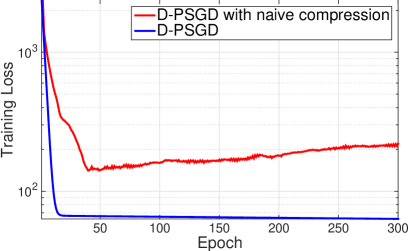
Figure 1: D-PSGD vs. D-PSGD with naive compression

3 Preliminary: decentralized parallel stochastic gradient descent (D-PSGD)

Unlike the traditional (centralized) parallel stochastic gradient descent (C-PSGD), which requires a central node to compute the average value of all leaf nodes, the decentralized parallel stochastic gradient descent (D-PSGD) algorithm does not need such a central node. Each node (say node $i$) only exchanges its local model $\bm{x}^{(i)}$ with its neighbors to take weighted average, specifically, $\bm{x}^{(i)}=\sum_{j=1}^{n}W_{ij}\bm{x}^{(j)}$ where $W_{ij}\geq 0$ in general and $W_{ij}=0$ means that node $i$ and node $j$ is not connected. At $t$th iteration, D-PSGD consists of three steps ($i$ is the node index):

1. Each node computes the stochastic gradient $\nabla F_{i}(\bm{x}^{(i)}_{t};\xi_{t}^{(i)})$, where $\xi^{(i)}_{t}$ is the samples from its local data set and $\bm{x}^{(i)}_{t}$ is the local model on node $i$.

2. Each node queries its neighbors’ variables and updates its local model using $\bm{x}^{(i)}=\sum_{j=1}^{n}W_{ij}\bm{x}^{(j)}$.

3. Each node updates its local model $\bm{x}^{(i)}_{t}\leftarrow\bm{x}^{(i)}_{t}-\gamma_{t}\nabla F_{i}\left(\bm{x}_{t}^{(i)};\xi^{(i)}_{t}\right)$ using stochastic gradient, where $\gamma_{t}$ is the learning rate.

To look at the D-PSGD algorithm from a global view, by defining

$$X:=[\bm{x}^{(1)},\bm{x}^{(2)},\cdots,\bm{x}^{(n)}]\in\mathbb{R}^{N\times n},\quad G(X;\xi):=[\nabla F_{1}(x^{(1)};\xi^{(1)}),\cdots,\nabla F_{n}(x^{(n)};\xi^{(n)})]$$

$$\nabla f(\overline{X}):=\sum_{i=1}^{n}\frac{1}{n}\nabla f_{i}\left(\frac{1}{n}\sum_{i=1}^{n}x^{(i)}\right),\quad\overline{\nabla f}(X):=\mathbb{E}_{\xi}G(X;\xi_{t})\frac{\bm{1}}{n}=\frac{1}{n}\sum_{i=1}^{n}\nabla f_{i}(x^{(i)}),$$

the D-PSGD can be summarized into the form $X_{t+1}=X_{t}W-\gamma_{t}G(X_{t};\xi_{t})$.

The convergence rate of D-PSGD can be shown to be $O\left(\frac{\sigma}{\sqrt{nT}}+\frac{n^{\frac{1}{3}}\zeta^{\frac{2}{3}}}{T^{\frac{2}{3}}}\right)$ (without assuming convexity) where both $\sigma$ and $\zeta$ are the stochastic variance (please refer to Assumption 1 for detailed definitions), if the learning rate is chosen appropriately.

4 Quantized, Decentralized Algorithms

We introduce two quantized decentralized algorithms that compress information exchanged between nodes. All communications for decentralized algorithms are exchanging local models $\bm{x}^{(i)}$.

To reduce the communication cost, a straightforward idea is to compress the information exchanged within the decentralized network just like centralized algorithms sending compressed stochastic gradient (Alistarh et al., 2017). Unfortunately, such naive combination does not work even using the unbiased stochastic compression and diminishing learning rate as shown in Figure 1. The reason can be seen from the detailed derivation (please find it in Supplement).

Before propose our solutions to this issue, let us first make some common optimization assumptions for analyzing decentralized stochastic algorithms (Lian et al., 2017b).

Assumption 1.

Throughout this paper, we make the following commonly used assumptions:

1. Lipschitzian gradient: All function $f_{i}(\cdot)$’s are with $L$-Lipschitzian gradients.

2. Symmetric double stochastic matrix: The weighted matrix $W$ is a real double stochastic matrix that satisfies $W=W^{\top}$ and $W\bm{1}=W$.

3. Spectral gap: Given the symmetric doubly stochastic matrix $W$, we define $\rho:=\max\{|\lambda_{2}(W)|,|\lambda_{n}(W)|\}$ and assume $\rho<1$.

4. Bounded variance: Assume the variance of stochastic gradient to be bounded

   $$\mathbb{E}_{\xi\sim\mathcal{D}_{i}}\left\|\nabla F_{i}(\bm{x};\xi)-\nabla f_{i}(\bm{x})\right\|^{2}\leqslant\sigma^{2},\quad{1\over n}\sum_{i=1}^{n}\left\|\nabla f_{i}(\bm{x})-\nabla f(\bm{x})\right\|^{2}\leqslant\zeta^{2},\quad\forall i,\forall\bm{x},$$

5. Independent and unbiased stochastic compression: The stochastic compression operation $\bm{C}(\cdot)$ is unbiased, that is, $\mathbb{E}(\bm{C}(Z))=Z$ for any $Z$ and the stochastic compressions are independent on different workers or at different time point.

The last assumption essentially restricts the compression to be lossy but unbiased. Biased stochastic compression is generally hard to ensure the convergence and lossless compression can combine with any algorithms. Both of them are beyond of the scope of this paper. The commonly used stochastic unbiased compression include random quantization (Zhang et al., 2017a) and sparsification (Wangni et al., 2017; Konečnỳ and Richtárik, 2016).

4.1 Difference compression approach

Algorithm 1 DCD-PSGD

1: Input: Initial point $\bm{x}^{(i)}_{1}=\bm{x}_{1}$, initial replica $\hat{\bm{x}}^{(i)}_{1}=\bm{x}_{1}$, iteration step length $\gamma$, weighted matrix $W$, and number of total iterations T

2: for t = 1,2,…,T do

3:    Randomly sample $\xi^{(i)}_{t}$ from local data of the $i$th node

4:    Compute local stochastic gradient $\nabla F_{i}(\bm{x}^{(i)}_{t};\xi^{(i)}_{t})$ using $\xi^{(i)}_{t}$ and current optimization variable $\bm{x}^{(i)}_{t}$

5:     Update the local model using local stochastic gradient and the weighted average of its connected neighbors’ replica (denote as $\hat{\bm{x}}^{(j)}_{t}$):

$$\bm{x}_{t+\frac{1}{2}}^{(i)}=\sum_{j=1}^{n}W_{ij}\bm{x}^{(j)}_{t}-\gamma\nabla F_{i}(\bm{x}^{(i)}_{t};\xi^{(i)}_{t}),$$

6:    Each node computes $\bm{z}^{(i)}_{t}=\bm{x}_{t+{1\over 2}}^{(i)}-\bm{x}^{(i)}_{t},$ and compress this $\bm{z}^{(i)}_{t}$ into $\bm{C}(\bm{z}_{t}^{(i)})$.

7:    Update the local optimization variables

$$\bm{x}_{t+1}^{(i)}\leftarrow\bm{x}_{t}^{(i)}+\bm{C}(\bm{z}_{t}^{(i)}).$$

8:    Send $\bm{C}(\bm{z}_{t}^{(i)})$ to its connected neighbors, and update the replicas of its connected neighbors’ values:

$$\hat{\bm{x}}_{t+1}^{(j)}=\hat{\bm{x}}_{t}^{(j)}+\bm{C}(\bm{z}_{t}^{(i)}).$$

9: end for

10: Output: $\frac{1}{n}\sum_{i=1}^{n}\bm{x}^{(i)}_{T}$

Algorithm 2 ECD-PSGD

1: Input: Initial point $\bm{x}^{(i)}_{1}=\bm{x}_{1}$, initial estimate ${\color[rgb]{0,0,0}\tilde{\bm{x}}}^{(i)}_{1}=\bm{x}_{1}$, iteration step length $\gamma$, weighted matrix $W$, and number of total iterations T.

2: for $t=1,2,\cdots,T$ do

3:    Randomly sample $\xi^{(i)}_{t}$ from local data of the $i$th node

4:    Compute local stochastic gradient $\nabla F_{i}(\bm{x}^{(i)}_{t};\xi^{(i)}_{t})$ using $\xi^{(i)}_{t}$ and current optimization variable $\bm{x}^{(i)}_{t}$

5:    Compute the neighborhood weighted average by using the estimate value of the connected neighbors :

$$\bm{x}_{t+\frac{1}{2}}^{(i)}=\sum_{j=1}^{n}W_{ij}{\color[rgb]{0,0,0}\tilde{\bm{x}}}^{(j)}_{t}$$

6:    Update the local model

$$\bm{x}_{t+1}^{(i)}\leftarrow\bm{x}_{t+\frac{1}{2}}^{(i)}-\gamma\nabla F_{i}(\bm{x}^{(i)}_{t},\xi^{(i)}_{t})$$

7:    Each node computes the $z$-value of itself:

$$\bm{z}^{(i)}_{t+1}=\left(1-0.5t\right)\bm{x}_{t}^{(i)}+0.5t\bm{x}_{t+1}^{(i)}$$

and compress this $\bm{z}^{(i)}_{t}$ into $\bm{C}(\bm{z}_{t}^{(j)})$.

8:    Each node updates the estimate for its connected neighbors:

$${\color[rgb]{0,0,0}\tilde{\bm{x}}}_{t+1}^{(j)}=\left(1-2t^{-1}\right){\color[rgb]{0,0,0}\tilde{\bm{x}}}^{(j)}_{t}+2t^{-1}\bm{C}(\bm{z}_{t}^{(j)})$$

9: end for

10: Output: $\frac{1}{n}\sum_{i=1}^{n}\bm{x}^{(i)}_{T}$

In this section, we introduces a difference based approach, namely, difference compression D-PSGD (DCD-PSGD), to ensure efficient convergence.

The DCD-PSGD basically follows the framework of D-PSGD, except that nodes exchange the compressed difference of local models between two successive iterations, instead of exchanging local models. More specifically, each node needs to store its neighbors’ models in last iteration $\{{\color[rgb]{0,0,0}{\hat{\bm{x}}}^{(j)}_{t}}:j~{}\text{is node $i$'s neighbor}\}$ and follow the following steps:

1. take the weighted average and apply stochastic gradient descent step: $\bm{x}_{t+\frac{1}{2}}^{(i)}=\sum_{j=1}^{n}W_{ij}{{\color[rgb]{0,0,0}\hat{\bm{x}}}^{(j)}_{t}}-\gamma\nabla F_{i}(\bm{x}^{(i)}_{t};\xi^{(i)}_{t})$, where $\hat{\bm{x}}^{(j)}_{t}$ is just the replica of $\bm{x}^{(j)}_{t}$ but is stored on node $i$;

2. compress the difference between $\bm{x}^{(i)}_{t}$ and $\bm{x}_{t+\frac{1}{2}}^{(i)}$ and update the local model:$\bm{z}_{t}^{(i)}=\bm{x}_{t+\frac{1}{2}}^{(i)}-\bm{x}_{t}^{(i)},\quad\bm{x}^{(i)}_{t+1}=\bm{x}^{(i)}_{t}+\bm{C}(\bm{z}_{t}^{(i)})$;

3. send $\bm{C}(\bm{z}_{t}^{(i)})$ and query neighbors’ $\bm{C}(\bm{z}_{t})$ to update the local replica: $\forall j~{}\text{is node $i$'s neighbor}$, $\hat{\bm{x}}_{t+1}^{(j)}=\hat{\bm{x}}^{(j)}_{t}+\bm{C}(\bm{z}_{t}^{(j)})$.

The full DCD-PSGD algorithm is described in Algorithm 1.

To ensure convergence, we need to make some restriction on the compression operator $\bm{C}(\cdot)$. Again this compression operator could be random quantization or random sparsification or any other operators. We introduce the definition of the signal-to-noise related parameter $\alpha$. Let $\alpha:=\sqrt{\sup_{Z\neq 0}{\|Q\|^{2}_{F}/\|Z\|^{2}_{F}}}$, where $Q=Z-C(Z)$. We have the following theorem.

Theorem 1.

Under the Assumption 1, if $\alpha$ satisfies $(1-\rho)^{2}-4\mu^{2}\alpha^{2}>0$, choosing $\gamma$ satisfying $1-3D_{1}L^{2}\gamma^{2}>0$, we have the following convergence rate for Algorithm 1

$$\sum_{t=1}^{T}\left(\left(1-D_{3}\right)\mathbb{E}\|\nabla f(\overline{X}_{t})\|^{2}+D_{4}\mathbb{E}\|\overline{\nabla f}(X_{t})\|^{2}\right)\leq\frac{2(f(0)-f^{*})}{\gamma}+\frac{L\gamma T\sigma^{2}}{n}$$

$$+\left(\frac{T\gamma^{2}LD_{2}}{2}+\frac{\left(4L^{2}+3L^{3}D_{2}\gamma^{2}\right)D_{1}T\gamma^{2}}{1-3D_{1}L^{2}\gamma^{2}}\right)\sigma^{2}+\frac{\left(4L^{2}+3L^{3}D_{2}\gamma^{2}\right)3D_{1}T\gamma^{2}}{1-3D_{1}L^{2}\gamma^{2}}\zeta^{2},$$ (2)

where $\mu:=\max_{i\in\{2,\cdots,n\}}|\lambda_{i}-1|$, and

$$D_{1}:=\frac{2\alpha^{2}}{1-\rho^{2}}\left(\frac{2\mu^{2}(1+2\alpha^{2})}{(1-\rho)^{2}-4\mu^{2}\alpha^{2}}+1\right)+\frac{1}{(1-\rho)^{2}}, D_{2}:=2\alpha^{2}\left(\frac{2\mu^{2}(1+2\alpha^{2})}{(1-\rho)^{2}-4\mu^{2}\alpha^{2}}+1\right)$$

$$D_{3}:=\frac{\left(4L^{2}+3L^{3}D_{2}\gamma^{2}\right)3D_{1}\gamma^{2}}{1-3D_{1}L^{2}\gamma^{2}}+\frac{3LD_{2}\gamma^{2}}{2}, D_{4}:=\left(1-L\gamma\right).$$

To make the result more clear, we appropriately choose the steplength in the following:

Corollary 2.

Choose $\gamma=\left(6\sqrt{D_{1}}L+6\sqrt{D_{2}L}+\frac{\sigma}{\sqrt{n}}T^{\frac{1}{2}}+\zeta^{\frac{2}{3}}T^{\frac{1}{3}}\right)^{-1}$ in Algorithm 1. If $\alpha$ is small enough that satisfies $(1-\rho)^{2}-4\mu^{2}\alpha^{2}>0$, then we have

$$\frac{1}{T}\sum_{t=1}^{T}\mathbb{E}\|\nabla f(\overline{X}_{t})\|^{2}\lesssim \frac{\sigma}{\sqrt{nT}}+\frac{\zeta^{\frac{2}{3}}}{T^{\frac{2}{3}}}+\frac{1}{T}.$$

where $D_{1}$, $D_{2}$ follow to same definition in Theorem 1 and we treat $f(0)-f^{*}$, $L$, and $\rho$ constants.

The leading term of the convergence rate is $O\left(1/\sqrt{Tn}\right)$, and we also proved the convergence rate for $\mathbb{E}\left[\sum_{i=1}^{n}\left\|\overline{X}_{t}-\bm{x}_{t}^{(i)}\right\|^{2}\right]$ (see (27) in Supplementary). We shall see the tightness of our result in the following discussion.

Linear speedup

Since the leading term of the convergence rate is $O\left(1/\sqrt{Tn}\right)$ when $T$ is large, which is consistent with the convergence rate of C-PSGD, this indicates that we would achieve a linear speed up with respect to the number of nodes.

Consistence with D-PSGD

Setting $\alpha=0$ to match the scenario of D-PSGD, ECD-PSGD admits the rate $O\left(\frac{\sigma}{\sqrt{nT}}+\frac{\zeta^{\frac{2}{3}}}{T^{\frac{2}{3}}}\right)$, that is slightly better the rate of D-PSGD proved in Lian et al. (2017b) $O\left(\frac{\sigma}{\sqrt{nT}}+\frac{n^{\frac{2}{3}}\zeta^{\frac{2}{3}}}{T^{\frac{2}{3}}}\right)$. The non-leading terms’ dependence of the spectral gap $(1-\rho)$ is also consistent with the result in D-PSDG.

4.2 Extrapolation compression approach

From Theorem 1, we can see that there is an upper bound for the compressing level $\alpha$ in DCD-PSGD. Moreover, since the spectral gap $(1-\rho)$ would decrease with the growth of the amount of the workers, so DCD-PSGD will fail to work under a very aggressive compression. So in this section, we propose another approach, namely ECD-PSGD, to remove the restriction of the compressing degree, with a little sacrifice on the computation efficiency.

For ECD-PSGD, we make the following assumption that the noise brought by compression is bounded.

Assumption 2.

(Bounded compression noise) We assume the noise due to compression is unbiased and its variance is bounded, that is, $\forall\bm{z}\in\mathbb{R}^{n}$

$$\mathbb{E}\|\bm{C}(\bm{z})-\bm{z}\|^{2}\leq\tilde{\sigma}^{2}/2,\quad\forall\bm{z}$$

Instead of sending the local model $\bm{x}^{(i)}_{t}$ directly to neighbors, we send a $z$-value that is extrapolated from $\bm{x}^{(i)}_{t}$ and $\bm{x}^{(i)}_{t-1}$ at each iteration. Each node (say, node $i$) estimates its neighbor’s values $\bm{x}^{(j)}_{t}$ from compressed $z$-value at $t$-th iteration. This procedure could ensure diminishing estimate error, in particular, $\mathbb{E}\|\tilde{\bm{x}}^{(j)}_{t}-\bm{x}^{(j)}_{t}\|^{2}\leq\mathcal{O}\left(t^{-1}\right)$.

At $t$th iteration, node $i$ performs the following steps to estimate $\bm{x}^{(j)}_{t}$ by $\tilde{\bm{x}}^{(j)}_{t}$:

• The node $j$, computes the $z$-value that is obtained through extrapolation

  $$\bm{z}_{t}^{(j)}=\left(1-0.5t\right)\bm{x}_{t-1}^{(j)}+0.5t{\bm{x}}_{t}^{(j)},$$ (3)

• Compress $\bm{z}_{t}^{(j)}$ and send it to its neighbors, say node $i$. Node $i$ computes $\tilde{\bm{x}}_{t}^{(j)}$ using

  $$\tilde{\bm{x}}_{t}^{(j)}=\left(1-2t^{-1}\right)\tilde{\bm{x}}^{(j)}_{t-1}+2t^{-1}\bm{C}(\bm{z}_{t}^{(j)}).$$ (4)

Using Lemma 12 (see Supplemental Materials), if the compression noise ${\color[rgb]{0,0,0}\bm{q}}^{(j)}_{t}:=\bm{z}_{t}^{(i)}-\bm{C}(\bm{z}_{t}^{(i)})$ is globally bounded variance by $\tilde{\sigma}^{2}/2$, we will have

$$\mathbb{E}(\|\tilde{\bm{x}}^{(j)}_{t}-\bm{x}^{(j)}_{t}\|^{2})\leq\tilde{\sigma}^{2}/t.$$

Using this way to estimate the neighbors’ local models leads to the following equivalent updating form

$$X_{t+1}= \tilde{X}_{t}W-\gamma_{t}G(X_{t};\xi_{t})=X_{t}W+\underbrace{{Q}_{t}W}_{\text{diminished estimate error}}-\gamma_{t}G(X_{t};\xi_{t}).$$

The full extrapolation compression D-PSGD (ECD-PSGD) algorithm is summarized in Algorithm 2.

Below we will show that EDC-PSGD algorithm would admit the same convergence rate and the same computation complexity as D-PSGD.

Theorem 3 (Convergence of Algorithm 2).

Under Assumptions 1 and  2, choosing $\gamma_{t}$ in Algorithm 2 to be constant $\gamma$ satisfying $1-6C_{1}L^{2}\gamma^{2}>0$, we have the following convergence rate for Algorithm 2

$$\sum_{t=1}^{T}\left(\left(1-C_{3}\right)\mathbb{E}\|\nabla f(\overline{X}_{t})\|^{2}+C_{4}\mathbb{E}\|\overline{\nabla f}(X_{t})\|^{2}\right)$$

$$\leq \frac{2(f(0)-f^{*})}{\gamma}+\frac{L\log T}{n\gamma}\tilde{\sigma}^{2}+\frac{LT\gamma}{n}\sigma^{2}+\frac{4C_{2}\tilde{\sigma}^{2}L^{2}}{1-\rho^{2}}\log T+4L^{2}C_{2}\left(\sigma^{2}+3\zeta^{2}\right)C_{1}T\gamma^{2}.$$ (5)

where $C_{1}:=\frac{1}{(1-\rho)^{2}}$, $C_{2}:=\frac{1}{1-6\rho^{-2}C_{1}L^{2}\gamma^{2}}$, $C_{3}:=12L^{2}C_{2}C_{1}\gamma^{2}$, and $C_{4}:=1-L\gamma$.

To make the result more clear, we choose the steplength in the following:

Corollary 4.

In Algorithm 2 choose the steplength $\gamma=\left(12\sqrt{C_{1}}L+\frac{\sigma}{\sqrt{n}}T^{\frac{1}{2}}+\zeta^{\frac{2}{3}}T^{\frac{1}{3}}\right)^{-1}$. Then it admits the following convergence rate (with $f(0)-f^{*}$, $L$, and $\rho$ treated as constants).

$$\frac{1}{T}\sum_{t=1}^{T}\mathbb{E}\|\nabla f(\overline{X}_{t})\|^{2}\lesssim \frac{\sigma(1+\frac{\tilde{\sigma}^{2}\log T}{n})}{\sqrt{nT}}+\frac{\zeta^{\frac{2}{3}}(1+\frac{\tilde{\sigma}^{2}\log T}{n})}{T^{\frac{2}{3}}}+\frac{1}{T}+\frac{\tilde{\sigma}^{2}\log{T}}{T},$$ (6)

This result suggests the algorithm converges roughly in the rate $O({1/\sqrt{nT}})$, and we also proved the convergence rate for $\mathbb{E}\left[\sum_{i=1}^{n}\left\|\overline{X}_{t}-\bm{x}_{t}^{(i)}\right\|^{2}\right]$ (see (36) in Supplementary). The followed analysis will bring more detailed interpretation to show the tightness of our result.

Linear speedup

Since the leading term of the convergence rate is $O(1/\sqrt{nT})$ when $T$ is large, which is consistent with the convergence rate of C-PSGD, this indicates that we would achieve a linear speed up with respect to the number of nodes.

Consistence with D-PSGD

Setting $\tilde{\sigma}=0$ to match the scenario of D-PSGD, ECD-PSGD admits the rate $O\left(\frac{\sigma}{\sqrt{nT}}+\frac{\zeta^{\frac{2}{3}}}{T^{\frac{2}{3}}}\right)$, that is slightly better the rate of D-PSGD proved in Lian et al. (2017b) $O\left(\frac{\sigma}{\sqrt{nT}}+\frac{n^{\frac{1}{3}}\zeta^{\frac{2}{3}}}{T^{\frac{2}{3}}}\right)$. The non-leading terms’ dependence of the spectral gap $(1-\rho)$ is also consistent with the result in D-PSDG.

Comparison between DCD-PSGD and ECD-PSGD

On one side, in term of the convergence rate, ECD-PSGD is slightly worse than DCD-PSGD due to additional terms $\left(\frac{\sigma\tilde{\sigma}^{2}\log{T}}{n\sqrt{nT}}+\frac{\zeta^{\frac{2}{3}}\tilde{\sigma}^{2}\log{T}}{nT^{\frac{2}{3}}}+\frac{\tilde{\sigma}^{2}\log{T}}{T}\right)$ that suggests that if $\tilde{\sigma}$ is relatively large than $\sigma$, the additional terms dominate the convergence rate. On the other side, DCD-PSGD does not allow too aggressive compression or quantization and may lead to diverge due to $\alpha\leq\frac{1-\rho}{2\sqrt{2}\mu}$, while ECD-PSGD is quite robust to aggressive compression or quantization.

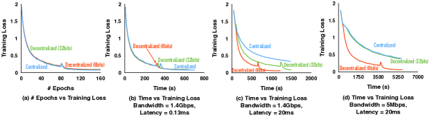
Figure 2: Performance Comparison between Decentralized and AllReduce implementations.

5 Experiments

In this section we evaluate two decentralized algorithms by comparing with an Allreduce implementation of centralized SGD. We run experiments under diverse network conditions and show that, decentralized algorithms with low precision can speed up training without hurting convergence.

5.1 Experimental Setup

We choose the image classification task as a benchmark to evaluate our theory. We train ResNet-20 (He et al., 2016) on CIFAR-10 dataset which has 50,000 images for training and 10,000 images for testing. Two proposed algorithms are implemented in Microsoft CNTK and compablack with CNTK’s original implementation of distributed SGD:

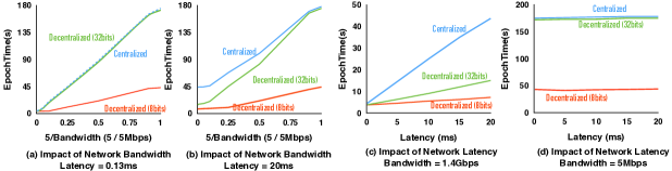
Figure 3: Performance Comparison in Diverse Network Conditions.

• Centralized: This implementation is based on MPI Allreduce primitive with full precision (32 bits). It is the standard training method for multiple nodes in CNTK.

• Decentralized_32bits/8bits: The implementation of the proposed decentralized approach with OpenMPI. The full precision is 32 bits, and the compressed precision is 8 bits.

• In this paper, we omit the comparison with quantized centralized training because the difference between Decentralized 8bits and Centralized 8bits would be similar to the original decentralized training paper Lian et al. (2017a) – when the network latency is high, decentralized algorithm outperforms centralized algorithm in terms of the time for each epoch.

We run experiments on 8 Amazon $p2.xlarge$ EC2 instances, each of which has one Nvidia K80 GPU. We use each GPU as a node. In decentralized cases, 8 nodes are connected as a ring topology, which means each node just communicates with its two neighbors. The batch size for each node is same as the default configuration in CNTK. We also tune learning rate for each variant.

5.2 Convergence and Run Time Performance

We first study the convergence of our algorithms. Figure 2(a) shows the convergence w.r.t # epochs of centralized and decentralized cases. We only show ECD-PSGD in the figure (and call it Decentralized) because DCD-PSGD has almost identical convergence behavior in this experiment. We can see that with our algorithms, decentralization and compression would not hurt the convergence rate.

We then compare the runtime performance. Figure 2(b, c, d) demonstrates how training loss decreases with the run time under different network conditions. We use $tc$ command to change bandwidth and latency of the underlying network. By default, 1.4 Gbps bandwidth and 0.13 ms latency is the best network condition we can get in this cluster. On this occasion, all implementations have a very similar runtime performance because communication is not the bottleneck for system. When the latency is high, as shown in 2(c), decentralized algorithms in both low and full precision can outperform the Allreduce method because of fewer number of communications. However, in low bandwidth case, training time is mainly dominated by the amount of communication data, so low precision method can be obviously faster than these full precision methods.

5.3 Speedup in Diverse Network Conditions

To better understand the influence of bandwidth and latency on speedup, we compare the time of one epoch under various of network conditions. Figure 3(a, b) shows the trend of epoch time with bandwidth decreasing from 1.4 Gbps to 5 Mbps. When the latency is low (Figure 3(a)), low precision algorithm is faster than its full precision counterpart because it only needs to exchange around one fourth of full precision method’s data amount. Note that although in a decentralized way, full precision case has no advantage over Allreduce in this situation, because they exchange exactly the same amount of data. When it comes to high latency shown in Figure 3(b), both full and low precision cases are much better than Allreduce in the beginning. But also, full precision method gets worse dramatically with the decline of bandwidth.

Figure 3(c, d) shows how latency influences the epoch time under good and bad bandwidth conditions. When bandwidth is not the bottleneck (Figure 3(c)), decentralized approaches with both full and low precision have similar epoch time because they have same number of communications. As is expected, Allreduce is slower in this case. When bandwidth is very low (Figure 3(d)), only decentralized algorithm with low precision can achieve best performance among all implementations.

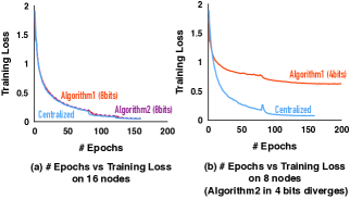
Figure 4: Comparison of Alg. 1 and Alg. 2

5.4 Discussion

Our previous experiments validate the efficiency of the decentralized algorithms on 8 nodes with 8 bits. However, we wonder if we can scale it to more nodes or compress the exchanged data even more aggressively. We firstly conducted experiments on 16 nodes with 8 bits as before. According to Figure 4(a), Alg. 1 and Alg. 2 on 16 nodes can still achieve basically same convergence rate as Allreduce, which shows the scalability of our algorithms. However, they can not be comparable to Allreduce with 4 bits, as is shown in 4(b). What is noteworthy is that these two compression approaches have quite different behaviors in 4 bits. For Alg. 1, although it converges much slower than Allreduce, its training loss keeps reducing. However, Alg. 2 just diverges in the beginning of training. This observation is consistent with our theoretical analysis.

6 Conclusion

In this paper, we studied the problem of combining two tricks of training distributed stochastic gradient descent under imperfect network conditions: quantization and decentralization. We developed two novel algorithms or quantized, decentralized training, analyze the theoretical property of both algorithms, and empirically study their performance in a various settings of network conditions. We found that when the underlying communication networks has both high latency and low bandwidth, quantized, decentralized algorithm outperforms other strategies significantly.

Supplemental Materials: Proofs

For the convenience of analysis, let us reformulate the updating rule of both proposed algorithms. Both algorithms can be generalized into the following form

$$X_{t+1}=X_{t}W-\gamma_{t}G(X_{t};\xi_{t})+Q_{t},$$ (7)

where $Q_{t}$ is the noise caused by compression.

More specifically, for ECD-PSGD, from (3) and (4), we have

$$Q_{t}= \tilde{X}_{t}-X_{t},$$

where $\tilde{X}_{t}$ is the estimation of $X_{t}$ computed using extrapolation. For DCD-PSGD, from (LABEL:alg2_globalevolution), we have

$$\Delta X_{t}:= X_{t}W-\gamma F(X_{t};\xi_{t})-X_{t}$$

$$Q_{t}= \bm{C}\left(\Delta X_{t}\right)-\Delta X_{t},$$

where $\bm{C}(\cdot)$ is the compression operator.

Proof organization

In section A, we first provide the properties of updating rule (7). Sections C and B will next specify $Q_{t}$ and show the upper bounds for $\|Q_{t}\|^{2}$ in Algorithms 2 and 1 respectively.

Notations

We define some additional notations throughout the following proof

$$\overline{X}_{t}:= X_{t}\frac{\bm{1}}{n}=\frac{1}{n}\sum_{i=1}^{n}\bm{x}_{t}^{(i)},$$

$$\overline{Q}_{t}:= Q_{t}\frac{\bm{1}}{n}=\frac{1}{n}\sum_{i=1}^{n}\bm{q}_{t}^{(i)},$$

$$\overline{G}(X_{t};\xi_{t}):= G(X_{t},\xi_{t})\frac{\bm{1}}{n}=\frac{1}{n}\sum_{i=1}^{n}\nabla F_{i}(\bm{x}_{t}^{(i)};\xi_{t}^{(i)}).$$

Appendix A General bound with compression noise

In this section, to see the influence of the compression more clearly, we are going to prove two general bounds (see see Lemma 7 and Lemma 8) for compressed D-PSGD that has the same updating rule like (7). Those bounds are very helpful for the following proof of our algorithms.

The most challenging part of a decentralized algorithm, unlike the centralized algorithm, is that we need to ensure the local model on each node to converge to the average value $\overline{X}_{t}$. So we start with an analysis of the quantity $\left\|\overline{X}_{t}-\bm{x}_{t}^{(i)}\right\|^{2}$ and its influence on the final convergence rate. For both ECD-PSGD and DCD-PSGD, we are going to prove that

$$\sum_{t=1}^{T}\sum_{i=1}^{n}\mathbb{E}\left\|\overline{X}_{t}-\bm{x}_{t}^{(i)}\right\|^{2}\leq \frac{2}{1-\rho^{2}}\sum_{t=1}^{T}\|Q_{t}\|^{2}_{F}+\frac{2}{(1-\rho)^{2}}\sum_{t=1}^{T}\gamma_{t}^{2}\|G(X_{t};\xi_{t})\|^{2}_{F},$$

and

$$\mathbb{E}\|\nabla f(\overline{X}_{t})\|^{2}+(1-L\gamma_{t})\mathbb{E}\|\overline{\nabla f}(X_{t})\|^{2}\leq \frac{2}{\gamma_{t}}\left(\mathbb{E}f(\overline{X}_{t})-\mathbb{E}f(\overline{X}_{t+1})\right)+\frac{L^{2}}{n}\mathbb{E}\sum_{i=1}^{n}\left\|\overline{X}_{t}-\bm{x}_{t}^{(i)}\right\|^{2}$$

$$+\frac{L}{\gamma_{t}}\mathbb{E}\|\overline{Q}_{t}\|^{2}+\frac{L\gamma_{t}}{n}\sigma^{2}.$$

From the above two inequalities, we can see that the extra noise term decodes the convergence efficiency of $\bm{x}_{t}^{(i)}$ to the average $\overline{X}_{t}$.

The proof of the general bound for (7) is divided into two parts. In subsection A.1, we provide a new perspective in understanding decentralization, which can be very helpful for the simplicity of our following proof. In subsection A.2, we give the detail proof for the general bound.

A.1 A more intuitive way to understand decentralization

To have a better understanding of how decentralized algorithms work, and how can we ensure a consensus from all local variables on each node. We provide a new perspective to understand decentralization using coordinate transformation, which can simplify our analysis in the following.

The confusion matrix $W$ satisfies $W=\sum_{i=1}^{n}\lambda_{i}\bm{v}^{i}\left(\bm{v}^{i}\right)^{\top}$ is doubly stochastic, so we can decompose it into $W=P\Lambda P^{\top}$, where $P=\left(\bm{v}^{1},\bm{v}^{2},\cdots,\bm{v}^{n}\right)$ that satisfies $P^{\top}P=PP^{\top}=I$. Without the loss of generality, we can assume $\lambda_{1}\geq\lambda_{2}\geq\cdots,\geq\lambda_{n}$. Then we have the following equalities:

$$X_{t+1}= X_{t}W-\gamma_{t}G(X_{t};\xi_{t})+Q_{t},$$

$$X_{t+1}= X_{t}P\Lambda P^{\top}-\gamma_{t}G(X_{t};\xi_{t})+Q_{t},$$

$$X_{t+1}P= X_{t}P\Lambda-G(X_{t};\xi_{t})P+Q_{t}P.$$

Consider the coordinate transformation using $P$ as the base change matrix, and denote $Y_{t}=X_{t}P$, $H(X_{t};\xi_{t})=G(X_{t};\xi_{t})P$, $R_{t}=Q_{t}P$. Then the above equation can be rewritten as

$$Y_{t+1}= Y_{t}\Lambda-H(X_{t};\xi_{t})+R_{t},.$$ (8)

Since $\Lambda$ is a diagonal matrix, so we use $\bm{y}_{t}^{(i)}$, $\bm{h}_{t}^{(i)}$, $\bm{r}_{t}^{(i)}$ to indicate the $i$-th column of $Y_{t}$, $H(X_{t};\xi_{t})$, $R_{t}$. Then (8) becomes

$$\bm{y}_{t+1}^{(i)}= \lambda_{i}\bm{y}_{t}^{(i)}-\bm{h}_{t}^{(i)}+\bm{r}_{t}^{(i)},\quad\forall i\in\{1,\cdots,n\}.$$ (9)

(9) offers us a much intuitive way to analysis the algorithm. Since all eigenvalues of $W$, except $\lambda_{1}$, satisfies $|\lambda_{i}|<1$, so the corresponding $\bm{y}_{t}^{(i)}$ would “decay to zero” due to the scaling factor $\lambda_{i}$.

Moreover, since the eigenvector corresponding to $\lambda_{1}$ is $\frac{1}{\sqrt{n}}(1,1,\cdots,1)$, then we have $\bm{y}_{t}^{(1)}=\overline{X}_{t}\sqrt{n}$. So, if $t\to\infty$, intuitively we can set $\bm{y}_{t}^{(i)}\to\bm{0}$ for $i\neq 1$, then $Y_{t}\to(\overline{X}_{t}\sqrt{n},0,\cdots,0)$ and $X_{t}\to\overline{X}_{t}\frac{\bm{1}}{n}$. This whole process shows how the confusion works under a coordinate transformation.

A.2 Analysis for the general updating form in (7)

Lemma 5.

For any matrix $X_{t}\in\mathbb{R}^{N\times n}$, decompose the confusion matrix $W$ as $W=\sum_{i=1}^{n}\lambda_{i}\bm{v}^{(i)}\left(\bm{v}^{(i)}\right)^{\top}=P\Lambda P^{\top}$, where $P=(\bm{v}^{(1)},\bm{v}^{(2)},\cdots,\bm{v}^{(n)})\in\mathbb{R}^{N\times n}$, $\bm{v}^{(i)}$ is the normalized eigenvector of $\lambda_{i}$, and $\Lambda$ is a diagonal matrix with $\lambda_{i}$ be its $i$th element. We have

$$\sum_{i=1}^{n}\left\|X_{t}W^{t}\bm{e}^{(i)}-X_{t}\frac{\bm{1}_{n}}{n}\right\|^{2}= \left\|X_{t}W^{t}-X_{t}\bm{v}^{(1)}\left(\bm{v}^{(1)}\right)^{\top}\right\|^{2}_{F}\leq\left\|\rho^{t}X_{t}\right\|^{2}_{F},$$

where $\rho$ follows the defination in Theorem 3.

Proof.

Since $W^{t}=P\Lambda^{t}P^{\top}$, we have

$$\sum_{i=1}^{n}\left\|X_{t}W^{t}\bm{e}^{(i)}-X_{t}\frac{\bm{1}_{n}}{n}\right\|^{2}= \sum_{i=1}^{n}\left\|\left(X_{t}W^{t}-X_{t}\frac{\bm{1}_{n}\bm{1}_{n}^{\top}}{n}\right)\bm{e}^{(i)}\right\|^{2}$$

$$= \left\|X_{t}W^{t}-X_{t}\bm{v}^{(1)}\left(\bm{v}^{(1)}\right)^{\top}\right\|^{2}_{F}$$

$$= \left\|X_{t}P\Lambda^{t}P^{\top}-X_{t}P\begin{pmatrix}1,0,\cdots,0\\ 0,0,\cdots,0\\ \cdots\\ 0,0,\cdots,0\end{pmatrix}P^{\top}\right\|^{2}_{F}$$

$$= \left\|X_{t}P\Lambda^{t}-X_{t}P\begin{pmatrix}1,0,\cdots,0\\ 0,0,\cdots,0\\ \cdots\\ 0,0,\cdots,0\end{pmatrix}\right\|^{2}_{F}$$

$$= \left\|X_{t}P\begin{pmatrix}&0,&0,&0,&\cdots,&0\\ &0,&\lambda_{2}^{t},&0,&\cdots,&0\\ &0,&0,&\lambda_{3}^{t},&\cdots,&0\\ &{5}\\ &0,&0,&0,&\cdots,&\lambda_{n}^{t}\end{pmatrix}\right\|^{2}_{F}$$

$$\leq \left\|\rho^{t}X_{t}P\right\|^{2}_{F}$$

$$= \left\|\rho^{t}X_{t}\right\|^{2}_{F}.$$

Specifically, when $t=0$, we have

$$\sum_{i=1}^{n}\left\|X_{t}\bm{e}^{(i)}-X_{t}\frac{\bm{1}_{n}}{n}\right\|^{2}= \left\|X_{t}P\begin{pmatrix}&0,&0,&0,&\cdots,&0\\ &0,&1,&0,&\cdots,&0\\ &0,&0,&1,&\cdots,&0\\ &{5}\\ &0,&0,&0,&\cdots,&1\end{pmatrix}\right\|^{2}_{F}$$

$$= \sum_{i=2}^{n}\left\|\bm{y}_{t}^{(i)}\right\|^{2},$$ (10)

where $\bm{y}_{t}^{(i)}=X_{t}P\bm{e^{(i)}}$. ∎

Lemma 6.

Given two non-negative sequences $\{a_{t}\}_{t=1}^{\infty}$ and $\{b_{t}\}_{t=1}^{\infty}$ that satisfying

$$a_{t}=\sum_{s=1}^{t}\rho^{t-s}b_{s},$$ (11)

with $\rho\in[0,1)$, we have

$$S_{k}:=\sum_{t=1}^{k}a_{t}\leq \sum_{s=1}^{k}\frac{b_{s}}{1-\rho},$$

$$D_{k}:=\sum_{t=1}^{k}a_{t}^{2}\leq \frac{1}{(1-\rho)^{2}}\sum_{s=1}^{k}b_{s}^{2}.$$

Proof.

From the definition, we have

$$S_{k}= \sum_{t=1}^{k}\sum_{s=1}^{t}\rho^{t-s}b_{s}=\sum_{s=1}^{k}\sum_{t=s}^{k}\rho^{t-s}b_{s}=\sum_{s=1}^{k}\sum_{t=0}^{k-s}\rho^{t}b_{s}\leq\sum_{s=1}^{k}{b_{s}\over 1-\rho},$$ (12)

$$D_{k}= \sum_{t=1}^{k}\sum_{s=1}^{t}\rho^{t-s}b_{s}\sum_{r=1}^{t}\rho^{t-r}b_{r}$$

$$= \sum_{t=1}^{k}\sum_{s=1}^{t}\sum_{r=1}^{t}\rho^{2t-s-r}b_{s}b_{r}$$

$$\leq \sum_{t=1}^{k}\sum_{s=1}^{t}\sum_{r=1}^{t}\rho^{2t-s-r}{b_{s}^{2}+b_{r}^{2}\over 2}$$

$$= \sum_{t=1}^{k}\sum_{s=1}^{t}\sum_{r=1}^{t}\rho^{2t-s-r}b_{s}^{2}$$

$$\leq {1\over 1-\rho}\sum_{t=1}^{k}\sum_{s=1}^{t}\rho^{t-s}b_{s}^{2}$$

$$\leq {1\over(1-\rho)^{2}}\sum_{s=1}^{k}b_{s}^{2}.\quad\text{(due to \eqref{eqn3})}$$

∎

Lemma 5 shows us an overall understanding about how the confusion matrix works, while Lemma 6 is a very important tool for analyzing the sequence in Lemma 5. Next we are going to give a upper bound for the difference between the local modes and the global mean mode.

Lemma 7.

Under Assumption 1, we have

$$\sum_{t=1}^{T}\sum_{i=1}^{n}\mathbb{E}\left\|\overline{X}_{t}-\bm{x}_{t}^{(i)}\right\|^{2}\leq \frac{2}{1-\rho^{2}}\sum_{t=1}^{T}\|Q_{s}\|^{2}_{F}+\frac{2}{(1-\rho)^{2}}\sum_{t=1}^{T}\gamma_{t}^{2}\|G(X_{t};\xi_{t})\|^{2}_{F}.$$

Proof.

From the updating rule, we have

$$X_{t}= \sum_{s=1}^{t-1}\gamma_{s}G\left(X_{s};\xi_{s}\right)W^{t-s-1}+\sum_{s=1}^{t-1}Q_{s}W^{t-s},$$

$$\overline{X}_{t}= \sum_{s=1}^{t-1}\gamma_{s}G\left(X_{s};\xi_{s}\right)W^{t-s-1}\frac{\bm{1}}{n}+\sum_{s=1}^{t-1}Q_{s}W^{t-s}\frac{\bm{1}}{n}$$

$$= \sum_{s=1}^{t-1}\gamma_{s}\overline{G}\left(X_{s};\xi_{s}\right)+\sum_{s=1}^{t-1}\overline{Q}_{s}.\quad\text{(due to $W\frac{\bm{1}}{n}=\frac{\bm{1}}{n}$)}$$

Therefore it yields

$$\sum_{i=1}^{n}\mathbb{E}\left\|\overline{X}_{t}-\bm{x}_{t}^{(i)}\right\|^{2}$$

$$= \sum_{i=1}^{n}\mathbb{E}\left\|\sum_{s=1}^{t-1}\left(Q_{s}W^{t-s}\bm{e}^{(i)}-\overline{Q}_{s}\right)-\sum_{s=1}^{t-1}\gamma_{s}\left(G(X_{s};\xi_{s})W^{t-s-1}\bm{e}^{(i)}-\overline{G}(X_{s};\xi_{s})\right)\right\|^{2}$$

$$\leq 2\sum_{i=1}^{n}\mathbb{E}\left\|\sum_{s=1}^{t-1}\left(Q_{s}W^{t-s}\bm{e}^{(i)}-\overline{Q}_{s}\right)\right\|^{2}+2\sum_{i=1}^{n}\mathbb{E}\left\|\sum_{s=1}^{t-1}\gamma_{s}\left(G(X_{s};\xi_{s})W^{t-s-1}\bm{e}^{(i)}-\overline{G}(X_{s};\xi_{s})\right)\right\|^{2}$$

$$= 2\sum_{i=1}^{n}\mathbb{E}\left\|\sum_{s=1}^{t-1}\left(Q_{s}W^{t-s}\bm{e}^{(i)}-\overline{Q}_{s}\right)\right\|^{2}+2\sum_{i=1}^{n}\mathbb{E}\left\|\sum_{s=1}^{t-1}\gamma_{s}\left(G(X_{s};\xi_{s})W^{t-s-1}\bm{e}^{(i)}-\overline{G}(X_{s};\xi_{s})\right)\right\|^{2}$$

$$= 2\sum_{i=1}^{n}\sum_{s=1}^{t-1}\mathbb{E}\left\|\left(Q_{s}W^{t-s}\bm{e}^{(i)}-\overline{Q}_{s}\right)\right\|^{2}+2\sum_{i=1}^{n}\mathbb{E}\left\|\sum_{s=1}^{t-1}\gamma_{s}\left(G(X_{s};\xi_{s})W^{t-s-1}\bm{e}^{(i)}-\overline{G}(X_{s};\xi_{s})\right)\right\|^{2}$$

$$+4\sum_{i=1}^{n}\sum_{s\neq s^{\prime}}\mathbb{E}\left\langle\mathbb{E}_{{}_{Q_{s}}}Q_{s}W^{t-s}\bm{e}^{(i)}-\mathbb{E}_{{}_{Q_{s}}}\overline{Q}_{s},\mathbb{E}_{{}_{Q_{s^{\prime}}}}Q_{s^{\prime}}W^{t-s^{\prime}}e^{(i)}-\mathbb{E}_{{}_{Q_{s^{\prime}}}}\overline{Q}_{s^{\prime}}\right\rangle$$

$$= 2\sum_{i=1}^{n}\sum_{s=1}^{t-1}\mathbb{E}\left\|\left(Q_{s}W^{t-s}\bm{e}^{(i)}-\overline{Q}_{s}\right)\right\|^{2}+2\sum_{i=1}^{n}\mathbb{E}\left\|\sum_{s=1}^{t-1}\gamma_{s}\left(G(X_{s};\xi_{s})W^{t-s-1}\bm{e}^{(i)}-\overline{G}(X_{s};\xi_{s})\right)\right\|^{2}$$

$$= 2\sum_{s=1}^{t-1}\mathbb{E}\left\|\left(Q_{s}W^{t-s}-Q_{s}\bm{v}_{1}\bm{v}_{1}^{\top}\right)\right\|^{2}_{F}+2\mathbb{E}\left\|\sum_{s=1}^{t-1}\gamma_{s}\left(G(X_{s};\xi_{s})W^{t-s-1}-G(X_{s};\xi_{s})\bm{v}_{1}\bm{v}_{1}^{\top}\right)\right\|^{2}_{F}$$

$$\leq 2\mathbb{E}\sum_{s=1}^{t-1}\left\|\rho^{t-s}Q_{s}\right\|^{2}_{F}+2\mathbb{E}\left(\sum_{s=1}^{t-1}\gamma_{s}\rho^{t-s-1}\left\|G(X_{s};\xi_{s})\right\|_{F}\right)^{2},\quad\text{(due to Lemma~{}\ref{lemma_bound_substract_mean})}$$

We can see that $\sum_{s=1}^{t-1}\rho^{2(t-s)}\left\|Q_{s}\right\|^{2}_{F}$ and $\sum_{s=1}^{t-1}\gamma_{s}\rho^{t-s-1}\left\|G(X_{s};\xi_{s})\right\|_{F}$ has the same structure with the sequence in Lemma 6, which leads to

$$\sum_{t=1}^{T}\sum_{i=1}^{n}\mathbb{E}\left\|\overline{X}_{t}-\bm{x}_{t}^{(i)}\right\|^{2}\leq \frac{2}{1-\rho^{2}}\mathbb{E}\sum_{t=1}^{T}\|Q_{s}\|^{2}_{F}+\frac{2}{(1-\rho)^{2}}\mathbb{E}\sum_{t=1}^{T}\gamma_{t}^{2}\|G(X_{t};\xi_{t})\|^{2}_{F}.$$

∎

Lemma 8.

Following the Assumption 1, we have

$$\frac{\gamma_{t}}{2}\mathbb{E}\|\nabla f(\overline{X}_{t})\|^{2}+(\frac{\gamma_{t}}{2}-\frac{L\gamma_{t}^{2}}{2})\mathbb{E}\|\overline{\nabla f}(X_{t})\|^{2}\leq \mathbb{E}f(\overline{X}_{t})-\mathbb{E}f(\overline{X}_{t+1})+\frac{L^{2}\gamma_{t}}{2n}\mathbb{E}\sum_{i=1}^{n}\left\|\overline{X}_{t}-\bm{x}_{t}^{(i)}\right\|^{2}$$

$$+\frac{L}{2}\mathbb{E}\|\overline{Q}_{t}\|^{2}+\frac{L\gamma_{t}^{2}}{2n}\sigma^{2}.$$ (13)

Proof.

From the updating rule, we have

$$X_{t+1}=\tilde{X}_{t}W-\gamma_{t}G(X_{t};\xi_{t})=X_{t}W+Q_{t}W-\gamma_{t}G(X_{t};\xi_{t}),$$

which implies

$$\overline{X}_{t+1}= \left(X_{t}W+Q_{t}W-\gamma_{t}G(X_{t};\xi_{t})\right)\frac{\bm{1}}{n}$$

$$=\frac{X_{t}\bm{1}}{n}+\frac{Q_{t}\bm{1}}{n}-\gamma_{t}\frac{G(X_{t};\xi_{t})\bm{1}}{n}$$

$$=\overline{X}_{t}+\overline{Q}_{t}-\gamma_{t}\overline{G}(X_{t};\xi_{t}).$$

From the Lipschitzian condition for the objective function $f_{i}$, we know that $f$ also satisfies the Lipschitzian condition. Then we have

$$\mathbb{E}f(\overline{X}_{t+1})$$

$$\leq \mathbb{E}f(\overline{X}_{t})+\mathbb{E}\left\langle\nabla f(\overline{X_{t}}),-\gamma_{t}\overline{G}(X_{t};\xi_{t})+\overline{Q}_{t}\right\rangle+\frac{L}{2}\mathbb{E}\left\|-\gamma_{t}\overline{G}(X_{t};\xi_{t})+\overline{Q}_{t}\right\|^{2}$$

$$= \mathbb{E}f(\overline{X}_{t})+\mathbb{E}\langle\nabla f(\overline{X}_{t}),-\gamma_{t}\overline{G}(X_{t};\xi_{t})+\mathbb{E}_{{}_{Q_{t}}}\overline{Q}_{t}\rangle$$

$$+\frac{L}{2}(\mathbb{E}\|\gamma_{t}\overline{G}(X_{t};\xi_{t})\|^{2}+\mathbb{E}\|\overline{Q}_{t}\|^{2}+\mathbb{E}\langle-\gamma_{t}\overline{G}(X_{t};\xi_{t}),\mathbb{E}_{{}_{Q_{t}}}\overline{Q}_{t}\rangle)$$

$$= \mathbb{E}f(\overline{X}_{t})+\mathbb{E}\langle\nabla f(\overline{X}_{t}),-\gamma_{t}\mathbb{E}_{\xi_{t}}\overline{G}(X_{t};\xi_{t})\rangle+\frac{L\gamma_{t}^{2}}{2}\mathbb{E}\|\overline{G}(X_{t};\xi_{t})\|^{2}+\frac{L}{2}\mathbb{E}\|\overline{Q}_{t}\|^{2}\quad\text{(due to $\mathbb{E}_{Q_{t}}\overline{Q}_{t}=\bm{0}$)}$$

$$= \mathbb{E}f(\overline{X}_{t})-\gamma_{t}\mathbb{E}\langle\nabla f(\overline{X}_{t}),\overline{\nabla f}(X_{t})\rangle+\frac{L\gamma_{t}^{2}}{2}\mathbb{E}\|(\overline{G}(X_{t};\xi_{t})-\overline{\nabla f}(X_{t}))+\overline{\nabla f}(X_{t})\|^{2}+\frac{L}{2}\mathbb{E}\|\overline{Q}_{t}\|^{2}$$

$$= \mathbb{E}f(\overline{X}_{t})-\gamma_{t}\mathbb{E}\langle\nabla f(\overline{X}_{t}),\overline{\nabla f}(X_{t})\rangle+\frac{L\gamma_{t}^{2}}{2}\mathbb{E}\|\overline{G}(X_{t};\xi_{t})-\overline{\nabla f}(X_{t})\|^{2}+\frac{L\gamma_{t}^{2}}{2}\mathbb{E}\|\overline{\nabla f}(X_{t})\|^{2}$$

$$+L\gamma_{t}^{2}\mathbb{E}\langle\mathbb{E}_{\xi_{t}}\overline{G}(X_{t};\xi_{t})-\overline{\nabla f}(X_{t}),\overline{\nabla f}(X_{t})\rangle+\frac{L}{2}\mathbb{E}\|\overline{Q}_{t}\|^{2}$$

$$= \mathbb{E}f(\overline{X}_{t})-\gamma_{t}\mathbb{E}\langle\nabla f(\overline{X}_{t}),\overline{\nabla f}(X_{t})\rangle+\frac{L\gamma_{t}^{2}}{2}\mathbb{E}\|\overline{G}(X_{t};\xi_{t})-\overline{\nabla f}(X_{t})\|^{2}$$

$$+\frac{L\gamma_{t}^{2}}{2}\mathbb{E}\|\overline{\nabla f}(X_{t})\|^{2}+\frac{L}{2}\mathbb{E}\|\overline{Q}_{t}\|^{2}$$

$$= \mathbb{E}f(\overline{X}_{t})-\gamma_{t}\mathbb{E}\langle\nabla f(\overline{X}_{t}),\overline{\nabla f}(X_{t})\rangle+\frac{L\gamma_{t}^{2}}{2n^{2}}\mathbb{E}\left\|\sum_{i=1}^{n}\left(\nabla F_{i}(x_{t}^{(i)};\xi_{t}^{(i)})-\nabla f_{i}(x_{t}^{(i)})\right)\right\|^{2}$$

$$+\frac{L\gamma_{t}^{2}}{2}\mathbb{E}\|\overline{\nabla f}(X_{t})\|^{2}+\frac{L}{2}\mathbb{E}\|\overline{Q}_{t}\|^{2}$$

$$= \mathbb{E}f(\overline{X}_{t})-\gamma_{t}\mathbb{E}\langle\nabla f(\overline{X}_{t}),\overline{\nabla f}(X_{t})\rangle+\frac{L\gamma_{t}^{2}}{2n^{2}}\sum_{i=1}^{n}\mathbb{E}\left\|\nabla F_{i}(x_{t}^{(i)};\xi_{t}^{(i)})-\nabla f_{i}(x_{t}^{(i)})\right\|^{2}$$

$$+\sum_{i\neq i^{\prime}}^{n}\mathbb{E}\left\langle\mathbb{E}_{\xi_{t}}\nabla F_{i}(x_{t}^{(i)};\xi_{t}^{(i)})-\nabla f_{i}(x_{t}^{(i)}),\nabla\mathbb{E}_{\xi_{t}}F_{i^{\prime}}(x_{t}^{(i^{\prime})};\xi_{t}^{(i^{\prime})})-\nabla f_{i^{\prime}}(x_{t}^{(i^{\prime})})\right\rangle$$

$$+\frac{L\gamma_{t}^{2}}{2}\mathbb{E}\|\overline{\nabla f}(X_{t})\|^{2}+\frac{L}{2}\mathbb{E}\|\overline{Q}_{t}\|^{2}$$

$$\leq \mathbb{E}f(\overline{X}_{t})-\gamma_{t}\mathbb{E}\langle\nabla f(\overline{X}_{t}),\overline{\nabla f}(X_{t})\rangle+\frac{L\gamma_{t}^{2}}{2n}\sigma^{2}+\frac{L\gamma_{t}^{2}}{2}\mathbb{E}\|\overline{\nabla f}(X_{t})\|^{2}+\frac{L}{2}\mathbb{E}\|\overline{Q}_{t}\|^{2}$$

$$= \mathbb{E}f(\overline{X}_{t})-\frac{\gamma_{t}}{2}\mathbb{E}\|\nabla f(\overline{X}_{t})\|^{2}-\frac{\gamma_{t}}{2}\mathbb{E}\|\overline{\nabla f}(X_{t})\|^{2}+\frac{\gamma_{t}}{2}\mathbb{E}\|\nabla f(\overline{X}_{t})-\overline{\nabla f}(X_{t})\|^{2}$$

$$+\frac{L\gamma_{t}^{2}}{2}\mathbb{E}\|\overline{\nabla f}(X_{t})\|^{2}+\frac{L}{2}\mathbb{E}\|\overline{Q}_{t}\|^{2}+\frac{L\gamma_{t}^{2}}{2n}\sigma^{2}\quad\text{(due to $2\langle\bm{a},\bm{b}\rangle=\|\bm{a}\|^{2}+\|\bm{b}\|^{2}-\|\bm{a}-\bm{b}\|^{2}$)}$$

$$= \mathbb{E}f(\overline{X}_{t})-\frac{\gamma_{t}}{2}\mathbb{E}\|\nabla f(\overline{X}_{t})\|^{2}-(\frac{\gamma_{t}}{2}-\frac{L\gamma_{t}^{2}}{2})\mathbb{E}\|\overline{\nabla f}(X_{t})\|^{2}+\frac{\gamma_{t}}{2}\mathbb{E}\|\nabla f(\overline{X}_{t})-\overline{\nabla f}(X_{t})\|^{2}$$

$$+\frac{L}{2}\mathbb{E}\|\overline{Q}_{t}\|^{2}+\frac{L\gamma_{t}^{2}}{2n}\sigma^{2}.$$ (14)

To estimate the upper bound for $\mathbb{E}\|\nabla f(\overline{X}_{t})-\overline{\nabla f}(X_{t})\|^{2}$, we have

$$\mathbb{E}\|\nabla f(\overline{X}_{t})-\overline{\nabla f}(X_{t})\|^{2}= \frac{1}{n^{2}}\mathbb{E}{\left\|\sum_{i=1}^{n}\left(\nabla f_{i}(\overline{X}_{t})-\nabla f_{i}(\bm{x}_{t}^{(i)})\right)\right\|^{2}}$$

$$\leq \frac{1}{n}\sum_{i=1}^{n}\mathbb{E}\left\|\nabla f_{i}(\overline{X}_{t})-\nabla f_{i}(\bm{x}_{t}^{(i)})\right\|^{2}$$

$$\leq \frac{L^{2}}{n}\mathbb{E}\sum_{i=1}^{n}\left\|\overline{X}_{t}-\bm{x}_{t}^{(i)}\right\|^{2}.$$ (15)

Combining (14) and (15) together, we have

$$\frac{\gamma_{t}}{2}\mathbb{E}\|\nabla f(\overline{X}_{t})\|^{2}+(\frac{\gamma_{t}}{2}-\frac{L\gamma_{t}^{2}}{2})\mathbb{E}\|\overline{\nabla f}(X_{t})\|^{2}\leq \mathbb{E}f(\overline{X}_{t})-\mathbb{E}f(\overline{X}_{t+1})+\frac{L^{2}\gamma_{t}}{2n}\mathbb{E}\sum_{i=1}^{n}\left\|\overline{X}_{t}-\bm{x}_{t}^{(i)}\right\|^{2}$$

$$+\frac{L}{2}\mathbb{E}\|\overline{Q}_{t}\|^{2}+\frac{L\gamma_{t}^{2}}{2n}\sigma^{2}.$$

which completes the proof. ∎

Appendix B Analysis for Algorithm 1

In Algorithm 1, we have

$$Z_{t}=X_{t}(W_{t}-I)-\gamma F\left(X_{t};\xi_{t}\right).$$ (16)

We will prove that

$$\sum_{t=1}^{T}E_{qt}\|Q_{t}\|^{2}_{F}\leq 2\alpha^{2}\left(\frac{2\mu^{2}(1+2\alpha^{2})}{(1-\rho)^{2}-4\mu^{2}\alpha^{2}}+1\right)\sum_{t=1}^{T}\gamma_{t}^{2}\|G\left(X_{t};\xi_{t}\right)\|^{2}_{F},$$

which leads to

$$\sum_{i=1}^{n}\sum_{t=1}^{T}\left(1-3D_{1}L^{2}\gamma_{t}^{2}\right)^{2}\mathbb{E}\left\|\overline{X}_{t}-\bm{x}_{t}^{(i)}\right\|^{2}\leq 2nD_{1}(\sigma^{2}+3\zeta^{2})\sum_{t=1}^{T}\gamma_{t}^{2}+6nD_{1}\sum_{t=1}^{T}\gamma_{t}^{2}\mathbb{E}\left\|\nabla f(\overline{X}_{t})\right\|^{2}.$$

$D_{1}$, $\mu$ and $\rho$ are defined in Theorem 1.

Lemma 9.

Under Assumption 1, when using Algorithm 1, we have

$$\sum_{t=1}^{T}E_{qt}\|Q_{t}\|^{2}_{F}\leq 2\alpha^{2}\left(\frac{2\mu^{2}(1+2\alpha^{2})}{(1-\rho)^{2}-4\mu^{2}\alpha^{2}}+1\right)\sum_{t=1}^{T}\gamma_{t}^{2}\|G\left(X_{t};\xi_{t}\right)\|^{2}_{F}$$

when $(1-\rho)^{2}-4\mu^{2}\alpha^{2}>0$, where

$$\mu= \max_{i\in\{2\cdots n\}}|\lambda_{i}-1|$$

Proof.

In the proof below, we use $[A]^{(i,j)}$ to indicate the $(i,j)$ element of matrix $A$.

For the noise induced by quantization, we have

$$\bm{r}_{t}^{(i)}=R_{t}\bm{e}^{(i)}=Q_{t}P\bm{e}^{(i)},$$

so

$$\|\bm{r}_{t}^{(i)}\|^{2}= \bm{e}^{(i)\top}P^{\top}Q_{t}^{\top}Q_{t}P\bm{e}^{(i)}$$

$$= \left(\bm{v}^{(i)}\right)^{\top}Q_{t}^{\top}Q_{t}\bm{v}^{(i)}.$$

As for $Q_{t}^{\top}Q_{t}$, the expectation of non-diagonal elements would be zero because the compression noise on node $i$ is independent on node $j$, which leads to

$$\mathbb{E}_{q_{t}}\left[Q_{t}^{\top}Q_{t}\right]^{(i,j)}= \mathbb{E}_{q_{t}}\sum_{k=1}^{N}Q_{t}^{(k,i)}Q_{t}^{(k,j)}$$

$$= \tau_{ij}\sum_{k=1}^{N}\mathbb{E}_{q_{t}}\left(Q_{t}^{(k,i)}\right)^{2},\quad\text{(due to $\mathbb{E}_{q_{t}}Q_{t}^{(k,i)}=0$ for $\forall i\in\{1\cdots n\}$)}$$

where $\tau_{ij}=1$ if $i=j$, else $\tau_{ij}=0$. Then

$$\mathbb{E}_{q_{t}}\|\bm{r}_{t}^{(i)}\|^{2}= \mathbb{E}_{q_{t}}\left(\bm{v}^{(i)}\right)^{\top}Q_{t}^{\top}Q_{t}\bm{v}^{(i)}$$

$$= \sum_{j=1}^{n}\sum_{k=1}^{N}\left(\bm{v}_{j}^{(i)}\right)^{2}\mathbb{E}_{q_{t}}\left(Q_{t}^{(k,j)}\right)^{2},$$

where $\bm{v}_{j}^{(i)}$ is the $j$th element of $\bm{v}^{(i)}$. So we have

$$\sum_{i=2}^{n}\mathbb{E}_{q_{t}}\|\bm{r}_{t}^{(i)}\|^{2}= \sum_{i=2}^{n}\sum_{j=1}^{n}\sum_{k=1}^{N}\left(\bm{v}_{j}^{(i)}\right)^{2}\mathbb{E}_{q_{t}}\left(Q_{t}^{(k,j)}\right)^{2}$$

$$\leq \sum_{i=1}^{n}\sum_{j=1}^{n}\sum_{k=1}^{N}\left(\bm{v}_{j}^{(i)}\right)^{2}\mathbb{E}_{q_{t}}\left(Q_{t}^{(k,j)}\right)^{2}$$

$$\leq \sum_{j=1}^{n}\sum_{k=1}^{N}\mathbb{E}_{q_{t}}\left(Q_{t}^{(k,j)}\right)^{2}\quad\text{(due to $\sum_{i=1}^{n}\left(\bm{v}_{j}^{(i)}\right)^{2}=1$)}$$

$$= \mathbb{E}_{q_{t}}\left\|Q_{t}\right\|^{2}_{F}.$$ (17)

$\mathbb{E}_{q_{t}}\left(Q_{t}^{(k,j)}\right)^{2}$ is the noise brought by quantization, which satisfies

$$\mathbb{E}_{q_{t}}\left(Q_{t}^{(k,j)}\right)^{2}\leq \alpha^{2}\left(z^{(k,j)}_{t}\right)^{2}$$

$$= \alpha^{2}\left(\left[X_{t}(W-I)\right]^{(k,j)}+[G\left(X_{t};\xi_{t}\right)]^{(k,j)}\right)^{2}\quad\text{(due to \eqref{global_z_t})}$$

$$= 2\alpha^{2}\left(\left[X_{t}(W-I)\right]^{(k,j)}\right)^{2}+2\alpha^{2}\left([G\left(X_{t};\xi_{t}\right)]^{(k,j)}\right)^{2}$$

$$= 2\alpha^{2}\left(\left[X_{t}P(\Lambda-I)P^{\top}\right]^{(k,j)}\right)^{2}+2\alpha^{2}\left([G\left(X_{t};\xi_{t}\right)]^{(k,j)}\right)^{2}$$

$$= 2\alpha^{2}\left(\left[Y(\Lambda-I)P^{\top}\right]^{(k,j)}\right)^{2}+2\alpha^{2}\left([G\left(X_{t};\xi_{t}\right)]^{(k,j)}\right)^{2},$$

then

$$\mathbb{E}_{q_{t}}\left\|Q_{t}\right\|^{2}_{F}\leq 2\alpha^{2}\left\|Y(\Lambda-I)P^{\top}\right\|^{2}_{F}+2\alpha^{2}\left\|G\left(X_{t};\xi_{t}\right)\right\|^{2}_{F}$$

$$= 2\alpha^{2}\left\|Y(\Lambda-I)\right\|^{2}_{F}+2\alpha^{2}\left\|G\left(X_{t};\xi_{t}\right)\right\|^{2}_{F}$$

$$= 2\alpha^{2}\left\|Y\begin{pmatrix}&0,&0,&\cdots,&0\\ &0,&\lambda_{2}-1,&\cdots,&0\\ &{4}\\ &0,&0,&\cdots,&\lambda_{n}-1\end{pmatrix}\right\|^{2}_{F}+2\alpha^{2}\left\|G\left(X_{t};\xi_{t}\right)\right\|^{2}_{F}$$

$$\leq 2\alpha^{2}\sum_{i=2}^{n}(\lambda_{i}-1)^{2}\|\bm{y}_{t}^{(i)}\|^{2}+2\alpha^{2}\left\|G\left(X_{t};\xi_{t}\right)\right\|^{2}_{F}$$

$$\leq 2\alpha^{2}\mu^{2}\sum_{i=2}^{n}\left\|\bm{y}_{t}^{(i)}\right\|^{2}+2\alpha^{2}\left\|G\left(X_{t};\xi_{t}\right)\right\|^{2}_{F}.\quad\text{(due to $\mu=\max_{i\in\{2\cdots n\}}|\lambda_{i}-1|$)}$$ (18)

Together with (17), it comes to

$$\sum_{i=2}^{n}\mathbb{E}_{q_{t}}\left\|\bm{r}_{t}^{(i)}\right\|^{2}\leq 2\alpha^{2}\mu^{2}\sum_{i=2}^{n}\left\|\bm{y}_{t}^{(i)}\right\|^{2}+2\alpha^{2}\left\|G\left(X_{t};\xi_{t}\right)\right\|^{2}_{F}.$$ (19)

From (9), we have

$$\bm{y}_{t}^{(i)}= \sum_{s=1}^{t-1}\lambda_{i}^{t-s-1}\left(-\bm{h}_{s}^{(i)}+\bm{r}_{s}^{(i)}\right),$$

$$\left\|\bm{y}_{t}^{(i)}\right\|^{2}\leq \left(\sum_{s=1}^{t-1}|\lambda_{i}|^{t-s-1}\left\|-\bm{h}_{s}^{(i)}+\bm{r}_{s}^{(i)}\right\|\right)^{2}.\quad\text{(due to $\|\bm{a}+\bm{b}\|^{2}\leq\|\bm{a}\|^{2}+\|\bm{b}\|^{2}$)}$$

Denote $m_{t}^{(i)}=\sum_{s=1}^{t-1}|\lambda_{i}|^{t-1-s}\left\|-\bm{h}_{s}^{(i)}+\bm{r}_{s}^{(i)}\right\|$, we can see that $m_{t}^{(i)}$ has the same structure of the sequence in Lemma 6, Therefore

$$\sum_{i=2}^{n}\sum_{t=1}^{T}\left(m_{t}^{(i)}\right)^{2}\leq \sum_{i=2}^{n}\sum_{t=1}^{T}\frac{1}{(1-|\lambda_{i}|)^{2}}\left\|-\bm{h}_{t}^{(i)}+\bm{r}_{t}^{(i)}\right\|^{2}$$

$$\leq \sum_{i=2}^{n}\sum_{t=1}^{T}\frac{2}{(1-|\lambda_{i}|)^{2}}\left(\left\|\bm{h}_{t}^{(i)}\right\|^{2}+\left\|\bm{r}_{t}^{(i)}\right\|^{2}\right)$$

$$= \sum_{i=2}^{n}\sum_{t=1}^{T}\frac{2}{(1-|\lambda_{i}|)^{2}}\left(\gamma_{t}^{2}\left\|G\left(X_{t};\xi_{t}\right)\bm{v}^{(i)}\right\|^{2}+\left\|\bm{r}_{t}^{(i)}\right\|^{2}\right)$$

$$= \sum_{i=2}^{n}\sum_{t=1}^{T}\frac{2\gamma_{t}^{2}\left\|G\left(X_{t};\xi_{t}\right)\bm{v}^{(i)}\right\|^{2}}{(1-|\lambda_{i}|)^{2}}+\sum_{i=2}^{n}\sum_{t=1}^{T}\frac{2}{(1-|\lambda_{i}|)^{2}}\left\|\bm{r}_{t}^{(i)}\right\|^{2}$$

$$\leq \sum_{i=2}^{n}\sum_{t=1}^{T}\frac{2\gamma_{t}^{2}\left\|G\left(X_{t};\xi_{t}\right)\bm{v}^{(i)}\right\|^{2}}{(1-|\lambda_{i}|)^{2}}+\sum_{i=2}^{n}\sum_{t=1}^{T}\frac{2}{(1-|\lambda_{i}|)^{2}}\left\|\bm{r}_{t}^{(i)}\right\|^{2}$$

$$\leq \frac{2}{(1-\rho)^{2}}\sum_{i=2}^{n}\sum_{t=1}^{T}\gamma_{t}^{2}\left\|G\left(X_{t};\xi_{t}\right)\bm{v}^{(i)}\right\|^{2}+\frac{2}{(1-\rho)^{2}}\sum_{i=2}^{n}\sum_{t=1}^{T}\left\|\bm{r}_{t}^{(i)}\right\|^{2}$$

$$\leq \frac{2}{(1-\rho)^{2}}\sum_{i=2}^{n}\sum_{t=1}^{T}\gamma_{t}^{2}\left\|G\left(X_{t};\xi_{t}\right)P\right\|^{2}+\frac{2}{(1-\rho)^{2}}\sum_{i=2}^{n}\sum_{t=1}^{T}\left\|\bm{r}_{t}^{(i)}\right\|^{2}$$

$$\leq \frac{2}{(1-\rho)^{2}}\sum_{t=1}^{T}\gamma_{t}^{2}\left\|G\left(X_{t};\xi_{t}\right)\right\|^{2}_{F}+\frac{2}{(1-\rho)^{2}}\sum_{i=2}^{n}\sum_{t=1}^{T}\left\|\bm{r}_{t}^{(i)}\right\|^{2}.$$ (20)

Combining (19) and (20) together, we have

$$\sum_{i=2}^{n}\sum_{t=1}^{T}\left\|\bm{y}_{t}^{(i)}\right\|^{2}\leq\sum_{i=2}^{n}\sum_{t=1}^{T}\left(m_{t}^{(i)}\right)^{2}\leq \frac{2(1+2\alpha^{2})}{(1-\rho)^{2}}\sum_{t=1}^{T}\gamma_{t}^{2}\left\|G\left(X_{t};\xi_{t}\right)\right\|^{2}_{F}+\frac{4\mu^{2}\alpha^{2}}{(1-\rho)^{2}}\sum_{l=2}^{n}\sum_{t=1}^{T}\left\|\bm{y}_{t}^{(l)}\right\|^{2},$$

It follows thtat

$$\sum_{i=2}^{n}\sum_{t=1}^{T}\left\|\bm{y}_{t}^{(i)}\right\|^{2}\leq \frac{2(1+2\alpha^{2})}{(1-\rho)^{2}}\sum_{t=1}^{T}\gamma_{t}^{2}\left\|G\left(X_{t};\xi_{t}\right)\right\|^{2}_{F}+\frac{4\mu^{2}\alpha^{2}}{(1-\rho)^{2}}\sum_{t=1}^{T}\sum_{l=2}^{n}\|\bm{y}_{t}^{(l)}\|^{2},$$

$$\left(1-\frac{4\mu^{2}\alpha^{2}}{(1-\rho)^{2}}\right)\sum_{i=2}^{n}\sum_{t=1}^{T}\left\|\bm{y}_{t}^{(i)}\right\|^{2}\leq \frac{2(1+2\alpha^{2})}{(1-\rho)^{2}}\sum_{t=1}^{T}\gamma_{t}^{2}\left\|G\left(X_{t};\xi_{t}\right)\right\|^{2}_{F}.$$

If $\alpha$ is small enough that satisfies $(1-\rho)^{2}-4\mu^{2}\alpha^{2}>0$, then we have

$$\sum_{i=2}^{n}\sum_{t=1}^{T}\left\|\bm{y}_{t}^{(i)}\right\|^{2}\leq \frac{2(1+2\alpha^{2})}{(1-\rho)^{2}-4\mu^{2}\alpha^{2}}\sum_{t=1}^{T}\gamma_{t}^{2}\left\|G\left(X_{t};\xi_{t}\right)\right\|^{2}_{F}.$$ (21)

Together (21) with (18) , we have

$$\sum_{t=1}^{T}E_{qt}\|Q_{t}\|^{2}_{F}\leq 2\alpha^{2}\mu^{2}\sum_{t=1}^{T}\sum_{l=2}^{n}\|\bm{y}_{t}^{(l)}\|^{2}+2\alpha^{2}\sum_{t=1}^{T}\gamma_{t}^{2}\left\|G\left(X_{t};\xi_{t}\right)\right\|^{2}_{F}$$

$$\leq 2\alpha^{2}\left(\frac{2\mu^{2}(1+2\alpha^{2})}{(1-\rho)^{2}-4\mu^{2}\alpha^{2}}+1\right)\sum_{t=1}^{T}\gamma_{t}^{2}\|G\left(X_{t};\xi_{t}\right)\|^{2}_{F}.$$

Moreover, setting $\gamma_{t}=\gamma$ and denote $2\alpha^{2}\left(\frac{2\mu^{2}(1+2\alpha^{2})}{(1-\rho)^{2}-4\mu^{2}\alpha^{2}}+1\right)=D_{2}$. Applying Lemma 12 to bound $\|G\left(X_{t};\xi_{t}\right)\|^{2}_{F}$, we have

$$\sum_{t=1}^{T}E_{qt}\|Q_{t}\|^{2}_{F}\leq n\sigma^{2}D_{2}\gamma^{2}T+3L^{2}D_{2}\gamma^{2}\sum_{i=1}^{n}\mathbb{E}\left\|\overline{X}_{t}-\bm{x}_{t}^{(i)}\right\|^{2}+3n\zeta^{2}D_{2}\gamma^{2}T$$

$$+3nD_{2}\gamma^{2}\mathbb{E}\sum_{t=1}^{T}\left\|\nabla f(\overline{X}_{t})\right\|^{2}.$$ (22)

∎

Lemma 10.

Under Assumption 1, we have

$$\sum_{i=1}^{n}\sum_{t=1}^{T}\left(1-3D_{1}L^{2}\gamma_{t}^{2}\right)^{2}\mathbb{E}\left\|\overline{X}_{t}-\bm{x}_{t}^{(i)}\right\|^{2}\leq 2nD_{1}(\sigma^{2}+3\zeta^{2})\sum_{t=1}^{T}\gamma_{t}^{2}+6nD_{1}\sum_{t=1}^{T}\gamma_{t}^{2}\mathbb{E}\left\|\nabla f(\overline{X}_{t})\right\|^{2}.$$

when $1-2\alpha^{2}\mu^{2}C_{\lambda}>0$, where

$$\mu= \max_{l\in\{2\cdots n\}}|\lambda_{l}-1|$$

$$\rho= \max_{l\in\{2\cdots n\}}|\lambda_{l}|$$

$$D_{1}= \frac{2\alpha^{2}}{1-\rho^{2}}\left(\frac{2\mu^{2}(1+2\alpha^{2})}{(1-\rho)^{2}-4\mu^{2}\alpha^{2}}+1\right)+\frac{1}{(1-\rho)^{2}}.$$

Proof.

From Lemma 7, we have

$$\sum_{t=1}^{T}\sum_{i=1}^{n}\mathbb{E}\left\|\overline{X}_{t}-\bm{x}_{t}^{(i)}\right\|^{2}$$

$$\leq \frac{2}{1-\rho^{2}}\sum_{t=1}^{T}\|Q_{s}\|^{2}_{F}+2\frac{1}{(1-\rho)^{2}}\sum_{t=1}^{T}\gamma_{t}^{2}\|G(X_{t};\xi_{t})\|^{2}_{F}$$

$$\leq 2\left(\frac{2\alpha^{2}}{1-\rho^{2}}\left(\frac{2\mu^{2}(1+2\alpha^{2})}{(1-\rho)^{2}-4\mu^{2}\alpha^{2}}+1\right)+\frac{1}{(1-\rho)^{2}}\right)\sum_{t=1}^{T}\gamma_{t}^{2}\|G(X_{t};\xi_{t})\|^{2}.\quad\text{(due to Lemma~{}\ref{lemma_bound_Q_t_alg2})}$$

Denote $\frac{2\alpha^{2}}{1-\rho^{2}}\left(\frac{2\mu^{2}(1+2\alpha^{2})}{(1-\rho)^{2}-4\mu^{2}\alpha^{2}}+1\right)+\frac{1}{(1-\rho)^{2}}=D_{1}$,then from Lemma 12, we have

$$\sum_{t=1}^{T}\sum_{i=1}^{n}\mathbb{E}\left\|\overline{X}_{t}-\bm{x}_{t}^{(i)}\right\|^{2}\leq 2nD_{1}(\sigma^{2}+3\zeta^{2})\sum_{t=1}^{T}\gamma_{t}^{2}+6nD_{1}\sum_{t=1}^{T}\gamma_{t}^{2}\mathbb{E}\left\|\nabla f(\overline{X}_{t})\right\|^{2}$$

$$+3D_{1}L^{2}\sum_{i=1}^{n}\gamma_{t}^{2}\mathbb{E}\left\|\overline{X}_{t}-\bm{x}_{t}^{(i)}\right\|^{2},$$

$$\sum_{t=1}^{T}\left(1-3D_{1}L^{2}\gamma_{t}^{2}\right)^{2}\sum_{i=1}^{n}\mathbb{E}\left\|\overline{X}_{t}-\bm{x}_{t}^{(i)}\right\|^{2}\leq 2nD_{1}(\sigma^{2}+3\zeta^{2})\sum_{t=1}^{T}\gamma_{t}^{2}+6nD_{1}\sum_{t=1}^{T}\gamma_{t}^{2}\mathbb{E}\left\|\nabla f(\overline{X}_{t})\right\|^{2}.$$

If $1-3D_{1}L^{2}\gamma_{t}^{2}>0$, then $\sum_{t=1}^{T}\sum_{i=1}^{n}\mathbb{E}\left\|\overline{X}_{t}-\bm{x}_{t}^{(i)}\right\|^{2}$ would be bounded. ∎

Proof to Theorem 1

Proof.

Combining Lemma 8 and (22), we have

$$\mathbb{E}\|\nabla f(\overline{X}_{t})\|^{2}+\left(1-L\gamma\right)\mathbb{E}\|\overline{\nabla f}(X_{t})\|^{2}\leq \frac{2}{\gamma}\left(\mathbb{E}f(\overline{X}_{t})-f^{*}-\left(\mathbb{E}f(\overline{X}_{(t+1)})-f^{*}\right)\right)$$

$$+\left(\frac{2L^{2}}{n}+\frac{3L^{3}D_{2}\gamma^{2}}{2n}\right)\sum_{i=1}^{n}\|\overline{X}_{t}-x_{t}^{(i)}\|^{2}$$

$$+\left(\frac{\gamma^{2}LD_{2}}{2}+\frac{L\gamma}{n}\right)T\sigma^{2}+\frac{3LD_{2}\gamma^{2}\zeta^{2}T}{2}$$

$$+\frac{3LD_{2}\gamma^{2}}{2}\mathbb{E}\left\|\nabla f(\overline{X}_{t})\right\|^{2}.$$ (23)

From Lemma 5, we have

$$\left(1-3D_{1}L^{2}\gamma^{2}\right)^{2}\sum_{t=1}^{T}\sum_{i=1}^{n}\mathbb{E}\left\|\overline{X}_{t}-\bm{x}_{t}^{(i)}\right\|^{2}\leq 2nD_{1}(\sigma^{2}+3\zeta^{2})T\gamma^{2}+6nD_{1}\gamma^{2}\sum_{t=1}^{T}\mathbb{E}\left\|\nabla f(\overline{X}_{t})\right\|^{2}.$$

If $\gamma$ is not too large that satisfies $1-3D_{1}L^{2}\gamma^{2}>0$, we have

$$\sum_{t=1}^{T}\sum_{i=1}^{n}\mathbb{E}\left\|\overline{X}_{t}-\bm{x}_{t}^{(i)}\right\|^{2}\leq \frac{2nD_{1}(\sigma^{2}+3\zeta^{2})T\gamma^{2}}{1-3D_{1}L^{2}\gamma^{2}}+\frac{6nD_{1}\gamma^{2}}{1-3D_{1}L^{2}\gamma^{2}}\sum_{t=1}^{T}\mathbb{E}\left\|\nabla f(\overline{X}_{t})\right\|^{2}.$$ (24)

Summarizing both sides of (23) and applying (24) yields

$$\sum_{t=1}^{T}\left(\mathbb{E}\|\nabla f(\overline{X}_{t})\|^{2}+\left(1-L\gamma\right)\mathbb{E}\|\overline{\nabla f}(X_{t})\|^{2}\right)$$

$$\leq \frac{2(f(0)-f^{*})}{\gamma}+\left(\frac{T\gamma^{2}LD_{2}}{2}+\frac{TL\gamma}{n}+\frac{\left(4L^{2}+3L^{3}D_{2}\gamma^{2}\right)D_{1}T\gamma^{2}}{1-3D_{1}L^{2}\gamma^{2}}\right)\sigma^{2}$$

$$+\frac{\left(4L^{2}+3L^{3}D_{2}\gamma^{2}\right)3D_{1}T\gamma^{2}}{1-3D_{1}L^{2}\gamma^{2}}\zeta^{2}+\frac{3LD_{2}\gamma^{2}T}{2}\zeta^{2}$$

$$+\left(\frac{\left(4L^{2}+3L^{3}D_{2}\gamma^{2}\right)3D_{1}\gamma^{2}}{1-3D_{1}L^{2}\gamma^{2}}+\frac{3LD_{2}\gamma^{2}}{2}\right)\sum_{t=1}^{T}\mathbb{E}\left\|\nabla f(\overline{X}_{t})\right\|^{2}.$$

It implies

$$\sum_{t=1}^{T}\left(\left(1-\frac{\left(4L^{2}+3L^{3}D_{2}\gamma^{2}\right)3D_{1}\gamma^{2}}{1-3D_{1}L^{2}\gamma^{2}}-\frac{3LD_{2}\gamma^{2}}{2}\right)\mathbb{E}\|\nabla f(\overline{X}_{t})\|^{2}+\left(1-L\gamma\right)\mathbb{E}\|\overline{\nabla f}(X_{t})\|^{2}\right)$$

$$\leq \frac{2(f(0)-f^{*})}{\gamma}+\left(\frac{T\gamma^{2}LD_{2}}{2}+\frac{L\gamma T}{n}+\frac{\left(4L^{2}+3L^{3}D_{2}\gamma^{2}\right)D_{1}T\gamma^{2}}{1-3D_{1}L^{2}\gamma^{2}}\right)\sigma^{2}$$

$$+\left(\frac{\left(4L^{2}+3L^{3}D_{2}\gamma^{2}\right)3D_{1}T\gamma^{2}}{1-3D_{1}L^{2}\gamma^{2}}+\frac{3LD_{2}\gamma^{2}T}{2}\right)\zeta^{2}.$$

Denote $D_{3}=\frac{\left(4L^{2}+3L^{3}D_{2}\gamma^{2}\right)3D_{1}\gamma^{2}}{1-3D_{1}L^{2}\gamma^{2}}+\frac{3LD_{2}\gamma^{2}}{2}$ and $D_{4}=1-L\gamma$, we have

$$\sum_{t=1}^{T}\left(\left(1-D_{3}\right)\mathbb{E}\|\nabla f(\overline{X}_{t})\|^{2}+D_{4}\mathbb{E}\|\overline{\nabla f}(X_{t})\|^{2}\right)$$

$$\leq \frac{2(f(0)-f^{*})}{\gamma}+\left(\frac{T\gamma^{2}LD_{2}}{2}+\frac{L\gamma T}{n}+\frac{\left(4L^{2}+3L^{3}D_{2}\gamma^{2}\right)D_{1}T\gamma^{2}}{1-3D_{1}L^{2}\gamma^{2}}\right)\sigma^{2}$$

$$+\left(\frac{\left(4L^{2}+3L^{3}D_{2}\gamma^{2}\right)3D_{1}T\gamma^{2}}{1-3D_{1}L^{2}\gamma^{2}}+\frac{3LD_{2}\gamma^{2}T}{2}\right)\zeta^{2}.$$

It completes the proof. ∎

Proof to Corollary 2

Proof.

Setting $\gamma=\frac{1}{6\sqrt{D_{1}}L+6\sqrt{D_{2}L}+\frac{\sigma}{\sqrt{n}}T^{\frac{1}{2}}+\zeta^{\frac{2}{3}}T^{\frac{1}{3}}}$, then we can verify

$$3D_{1}L^{2}\gamma^{2}\leq \frac{1}{12}$$

$$3LD_{2}\gamma^{2}\leq \frac{1}{12}$$

$$D_{3}\leq \frac{1}{2}$$

$$D_{4}\geq 0.$$

So we can remove the $\|\overline{\nabla f}(X_{t})\|^{2}$ on the LHS and substitute $(1-D_{3})$ with $\frac{1}{2}$. Therefore (2) becomes

$$\frac{1}{T}\sum_{t=1}^{T}\mathbb{E}\|\nabla f(\overline{X}_{t})\|^{2}\leq 4(f(0)-f^{*})\frac{\sigma}{\sqrt{Tn}}+\frac{4L\sigma}{\sqrt{Tn}}+\frac{\zeta^{\frac{2}{3}}}{T^{\frac{2}{3}}}(4LD_{2}+30L^{2}D_{1}+4(f(0)-f^{*}))$$

$$+\frac{n\sigma^{2}}{nD_{1}L^{2}+\sigma^{2}T}\left(5D_{1}L^{2}+\frac{LD_{2}}{2}\right)+\frac{4(f(0)-f^{*})(6\sqrt{D_{1}}L+6\sqrt{D_{2}L})}{T}.$$ (25)

From Lemma 10, we have

$$\frac{1}{T}\sum_{i=1}^{n}\sum_{t=1}^{T}\left(1-3D_{1}L^{2}\gamma^{2}\right)^{2}\mathbb{E}\left\|\overline{X}_{t}-\bm{x}_{t}^{(i)}\right\|^{2}\leq 2nD_{1}(\sigma^{2}+3\zeta^{2})\gamma^{2}+6nD_{1}\gamma^{2}\frac{1}{T}\sum_{t=1}^{T}\mathbb{E}\left\|\nabla f(\overline{X}_{t})\right\|^{2}$$

$$\leq \frac{2n\sqrt{n}D_{1}}{T}+\frac{6n\zeta^{\frac{2}{3}}}{T^{\frac{2}{3}}}+6nD_{1}\gamma^{2}\frac{1}{T}\sum_{t=1}^{T}\mathbb{E}\left\|\nabla f(\overline{X}_{t})\right\|^{2}.$$

$$\frac{1}{T}\sum_{i=1}^{n}\sum_{t=1}^{T}\mathbb{E}\left\|\overline{X}_{t}-\bm{x}_{t}^{(i)}\right\|^{2}\leq \frac{4n\sqrt{n}D_{1}}{T}+\frac{12n\zeta^{\frac{2}{3}}}{T^{\frac{2}{3}}}+12nD_{1}\gamma^{2}\frac{1}{T}\sum_{t=1}^{T}\mathbb{E}\left\|\nabla f(\overline{X}_{t})\right\|^{2}.$$ (26)

If $\alpha^{2}\leq\min\left\{\frac{(1-\rho)^{2}}{8\mu^{2}},\frac{1}{4}\right\}$, then

$$D_{2}= 2\alpha^{2}\left(\frac{2\mu^{2}(1+2\alpha^{2})}{(1-\rho)^{2}-4\mu^{2}\alpha^{2}}+1\right)\leq\frac{3\mu^{2}\alpha^{2}}{(1-\rho)^{2}}+2\alpha^{2},$$

$$D_{1}= \frac{D_{2}}{1-\rho^{2}}+\frac{1}{(1-\rho)^{2}}\leq\frac{D_{2}+1}{(1-\rho)^{2}},\quad\text{(due to $\rho<1$)}$$

which means $D_{2}=O\left(\alpha^{2}\right)$ and $D_{1}=O\left(\alpha^{2}+1\right)$.
So (26) becomes

$$\frac{1}{T}\sum_{t=1}^{T}\mathbb{E}\|\nabla f(\overline{X}_{t})\|^{2}\lesssim \frac{\sigma}{\sqrt{nT}}+\frac{\zeta^{\frac{2}{3}}(1+\alpha)}{T^{\frac{2}{3}}}+\frac{1+\alpha^{2}}{T}.$$

Combing the inequality above and (26), we have

$$\frac{1}{T}\sum_{i=1}^{n}\sum_{t=1}^{T}\mathbb{E}\left\|\overline{X}_{t}-\bm{x}_{t}^{(i)}\right\|^{2}\lesssim \frac{n\zeta^{\frac{2}{3}}}{T^{\frac{2}{3}}}+\frac{n\sqrt{n}(1+\alpha^{2})}{T}+\frac{n(1+\alpha)}{T^{2}}.$$ (27)

∎

Appendix C Analysis for Algorithm 2

We are going to prove that by using (3) and (4) in Algorithm 2, the upper bound for the compression noise would be

$$\mathbb{E}\|Q_{t}\|^{2}_{F}\leq\frac{n\tilde{\sigma}^{2}}{t}.$$

Therefore, combing this with Lemma 8 and Lemma 7, we would be able to prove the convergence rate for ALgorithm 2.

$$\sum_{t=1}^{T}\sum_{i=1}^{n}\left(1-6nC_{1}L^{2}\gamma_{t}^{2}\right)\mathbb{E}\left\|\overline{X}_{t}-x_{t}^{(i)}\right\|^{2}\leq \frac{2n^{2}\tilde{\sigma}^{2}}{1-\rho^{2}}\log T+2\left(\sigma^{2}+3\zeta^{2}\right)n^{2}C_{1}\sum_{t=1}^{T-1}\gamma_{t}^{2}$$

$$+6C_{1}n^{2}\sum_{t=1}^{T-1}\mathbb{E}\gamma_{t}^{2}\left\|\nabla f(\overline{X}_{t})\right\|^{2},$$

which ensures that all nodes would converge to the same value.

Lemma 11.

For any non-negative sequences $\{a_{n}\}_{n=1}^{+\infty}$ and $\{b_{n}\}_{n=1}^{+\infty}$ that satisfying

$$a_{t}=\left(1-\frac{2}{t}\right)^{2}a_{t-1}+\frac{4}{t^{2}}b_{t}$$

$$b_{t}\leq\frac{\tilde{\sigma}^{2}}{2}\quad\forall t\in\{1,2,3,\cdots\}$$

$$a_{1}=0,$$

we have

$$a_{t}\leq\frac{\tilde{\sigma}^{2}}{t}{\color[rgb]{1,0,0}.}$$

Proof.

We use induction to prove the lemma. Since $a_{1}=0\leq\tilde{\sigma}^{2}$, suppose the lemma holds for $t\leq k$, which means $a_{t}\leq\frac{\tilde{\sigma}^{2}}{t}$, for $\forall t\leq k$. Then it leads to

$$a_{k+1}= \left(1-\frac{2}{k}\right)^{2}a_{k}+\frac{4}{k^{2}}b_{t}$$

$$\leq \left(1-\frac{2}{k}\right)^{2}a_{k}+\frac{2\tilde{\sigma}^{2}}{k^{2}}$$

$$\leq \left(1-\frac{4}{k}+\frac{4}{k^{2}}\right)\frac{\tilde{\sigma}^{2}}{k}+\frac{2\tilde{\sigma}^{2}}{k^{2}}$$

$$= \tilde{\sigma}^{2}\left(\frac{1}{k}-\frac{1}{k+1}\right)-\frac{2\tilde{\sigma}^{2}}{k^{2}}+\frac{4\tilde{\sigma}^{2}}{k^{3}}+\frac{\tilde{\sigma}^{2}}{k+1}$$

$$= \frac{\tilde{\sigma}^{2}}{k^{2}(k+1)}\left(k-2(k+1)+\frac{4}{k}\right)+\frac{\tilde{\sigma}^{2}}{k+1}$$

$$= \frac{\tilde{\sigma}^{2}}{k^{2}(k+1)}\left(-k-2+\frac{4}{k}\right)+\frac{\tilde{\sigma}^{2}}{k+1}$$

$$\leq \frac{\tilde{\sigma}^{2}}{k+1}.\quad\text{(due to $k\geq 2$)}$$

It completes the proof. ∎

Lemma 12.

Under the Assumption 1, when using Algorithm 2, we have

$$\mathbb{E}\left\|G(X_{t},\xi_{t})\right\|^{2}_{F}\leq n\sigma^{2}+3L^{2}\sum_{i=1}^{n}\mathbb{E}\left\|\overline{X}_{t}-\bm{x}_{t}^{(i)}\right\|^{2}+3n\zeta^{2}+3n\mathbb{E}\left\|\nabla f(\overline{X}_{t})\right\|^{2},$$

$$\mathbb{E}\left\|Q_{t}\right\|^{2}_{F}\leq \frac{n\tilde{\sigma}^{2}}{t},$$

$$\mathbb{E}\left\|\overline{Q}_{t}\right\|^{2}_{F}\leq \frac{\tilde{\sigma}^{2}}{nt}.$$

Proof.

Notice that

$$\mathbb{E}\left\|G(X_{t},\xi_{t})\right\|^{2}_{F}=\sum_{i=1}^{n}\mathbb{E}\left\|\nabla F_{i}(x_{t}^{(i)};\xi_{t}^{(i)})\right\|^{2}.$$

We next estimate the upper bound of $\mathbb{E}\left\|\nabla F_{i}(\bm{x}_{t}^{(i)};\xi_{t}^{(i)})\right\|^{2}$ in the following

$$\mathbb{E}\left\|\nabla F_{i}(\bm{x}_{t}^{(i)};\xi_{t}^{(i)})\right\|^{2}= \mathbb{E}\left\|\left(\nabla F_{i}(\bm{x}_{t}^{(i)};\xi_{t}^{(i)})-\nabla f_{i}(\bm{x}_{t}^{(i)})\right)+\nabla f_{i}(\bm{x}_{t}^{(i)})\right\|^{2}$$

$$= \mathbb{E}\left\|\nabla F_{i}(\bm{x}_{t}^{(i)};\xi_{t}^{(i)})-\nabla f_{i}(\bm{x}_{t}^{(i)})\right\|^{2}+\mathbb{E}\left\|\nabla f_{i}(\bm{x}_{t}^{(i)})\right\|^{2}$$

$$+2\mathbb{E}\left\langle\mathbb{E}_{\xi_{t}}\nabla F_{i}(\bm{x}_{t}^{(i)};\xi_{t}^{(i)})-\nabla f_{i}(\bm{x}_{t}^{(i)}),\nabla f_{i}(\bm{x}_{t}^{(i)})\right\rangle$$

$$= \mathbb{E}\left\|\nabla F_{i}(\bm{x}_{t}^{(i)};\xi_{t}^{(i)})-\nabla f_{i}(\bm{x}_{t}^{(i)})\right\|^{2}+\mathbb{E}\left\|\nabla f_{i}(\bm{x}_{t}^{(i)})\right\|^{2}$$

$$\leq \sigma^{2}+\mathbb{E}\left\|\left(\nabla f_{i}(\bm{x}_{t}^{(i)})-\nabla f_{i}(\overline{X}_{t})\right)+\left(\nabla f_{i}(\overline{X}_{t})-\nabla f(\overline{X}_{t})\right)+\nabla f(\overline{X}_{t})\right\|^{2}$$

$$\leq \sigma^{2}+3\mathbb{E}\left\|\nabla f_{i}(\bm{x}_{t}^{(i)})-\nabla f_{i}(\overline{X}_{t})\right\|^{2}+3\mathbb{E}\left\|\nabla f_{i}(\overline{X}_{t})-\nabla f(\overline{X}_{t})\right\|^{2}$$

$$+3\mathbb{E}\left\|\nabla f(\overline{X}_{t})\right\|^{2}$$

$$\leq \sigma^{2}+3L^{2}\mathbb{E}\left\|X_{t}-\bm{x}_{t}^{(i)}\right\|^{2}+3\zeta^{2}+3\mathbb{E}\left\|\nabla f(\overline{X}_{t})\right\|^{2},$$

which means

$$\mathbb{E}\left\|G(X_{t},\xi_{t})\right\|^{2}\leq\sum_{i=1}^{n}\left\|\nabla F_{i}(\bm{x}_{t}^{(i)};\xi_{t}^{(i)})\right\|^{2}\leq n\sigma^{2}+3L^{2}\sum_{i=1}^{n}\mathbb{E}\left\|\overline{X}_{t}-\bm{x}_{t}^{(i)}\right\|^{2}+3n\zeta^{2}$$

$$+3n\mathbb{E}\left\|\nabla f(\overline{X}_{t})\right\|^{2}.$$

From (4), we have

$$\tilde{\bm{x}}^{(j)}_{t}-\bm{x}^{(j)}_{t}= (1-2t^{-1})(\tilde{\bm{x}}^{(j)}_{t-1}-\bm{x}^{(j)}_{t-1})+2t^{-1}\bm{q}^{(j)}_{t},$$ (28)

Then we have

$$\mathbb{E}\|\tilde{\bm{x}}^{(j)}_{t}-\bm{x}^{(j)}_{t}\|^{2}$$

$$= \left(1-2t^{-1}\right)^{2}\mathbb{E}\|\tilde{\bm{x}}^{(j)}_{t-1}-\bm{x}^{(j)}_{t-1}\|^{2}+4t^{-2}\mathbb{E}\|\bm{q}_{t}^{(j)}\|^{2}+2t^{-1}\left(1-2t^{-1}\right)\mathbb{E}\left\langle\tilde{\bm{x}}^{(j)}_{t-1}-\bm{x}^{(j)}_{t-1},\mathbb{E}_{\bm{q}_{t}^{(j)}}\bm{q}_{t}^{(j)}\right\rangle$$

Since $\mathbb{E}_{q_{t}^{(j)}}\bm{C}(\bm{z}_{t}^{(j)})=\bm{z}_{t}^{(j)}$, so we have $\mathbb{E}_{q_{t}^{(j)}}\bm{q}_{t}^{(j)}=0$, then

$$\mathbb{E}\|\tilde{\bm{x}}^{(j)}_{t}-\bm{x}^{(j)}_{t}\|^{2}=\left(1-2t^{-1}\right)^{2}\mathbb{E}\|\tilde{\bm{x}}^{(j)}_{t-1}-\bm{x}^{(j)}_{t-1}\|^{2}+4t^{-2}\mathbb{E}\|\bm{q_{t}^{(j)}}\|^{2}.$$ (29)

Meanwhile, (29) indicates that

$$\mathbb{E}\left\|\bm{q}_{t}^{(i)}\right\|^{2}\leq\left(1-\frac{2}{t}\right)^{2}\mathbb{E}\left\|\bm{q}_{t-1}^{(i)}\right\|^{2}+\frac{4}{t^{2}}\frac{\tilde{\sigma}^{2}}{2}.$$ (30)

So applying Lemma 12 into (30), we have

$$\mathbb{E}\left\|\bm{q}_{t}^{(i)}\right\|^{2}\leq\frac{\tilde{\sigma}^{2}}{t}.$$

Therefore

$$\mathbb{E}\left\|Q_{t}\right\|^{2}_{F}= \sum_{i=1}^{n}\mathbb{E}\left\|\bm{q}_{t}^{(i)}\right\|^{2}\leq\frac{n\tilde{\sigma}^{2}}{t},\quad\left(\text{due to $\mathbb{E}\left\|\bm{q}_{t}^{(i)}\right\|^{2}\leq\frac{\tilde{\sigma}^{2}}{t}$}\right)$$

$$\mathbb{E}\left\|\overline{Q}_{t}\right\|^{2}_{F}= \frac{1}{n^{2}}\mathbb{E}\left\|\sum_{i=1}^{n}\bm{q}_{t}^{(i)}\right\|^{2}$$

$$= \frac{1}{n^{2}}\sum_{i=1}^{n}\mathbb{E}\left\|\bm{q}_{t}^{(i)}\right\|^{2}+\sum_{i\neq i^{\prime}}^{n}\mathbb{E}\left\langle\bm{q}_{t}^{(i)},\bm{q}_{t}^{(i^{\prime})}\right\rangle$$

$$\leq \frac{\tilde{\sigma}^{2}}{nt}.\quad\left(\text{due to $\mathbb{E}\bm{q}_{t}^{(i)}=0$ for $\forall i\in\{1,\cdots,n\}$}\right)$$

∎

Lemma 13.

Under Assumption 1, when using Algorithm 2, we have

$$\sum_{t=1}^{T}\sum_{i=1}^{n}\left(1-6C_{1}L^{2}\gamma_{t}^{2}\right)\mathbb{E}\left\|\overline{X}_{t}-\bm{x}_{t}^{(i)}\right\|^{2}\leq \frac{2n\tilde{\sigma}^{2}}{1-\rho^{2}}\log T+2\left(\sigma^{2}+3\zeta^{2}\right)nC_{1}\sum_{t=1}^{T-1}\gamma_{t}^{2}$$

$$+6C_{1}n\sum_{t=1}^{T-1}\mathbb{E}\gamma_{t}^{2}\left\|\nabla f(\overline{X}_{t})\right\|^{2},$$ (31)

where $C_{1}$ is defined in Theorem 3.

Proof.

From Lemma 7 and Lemma 12, we have

$$\sum_{i=1}^{n}\sum_{t=1}^{T}\mathbb{E}\left\|\overline{X}_{t}-\bm{x}_{t}^{(i)}\right\|^{2}\leq \frac{2n\tilde{\sigma}^{2}}{1-\rho^{2}}\sum_{t=1}^{T-1}\frac{1}{t}+2C_{1}\sum_{t=1}^{T-1}\gamma_{t}^{2}\mathbb{E}\left\|G(X_{t};\xi_{t})\right\|^{2}$$

$$\leq \frac{2n\tilde{\sigma}^{2}}{1-\rho^{2}}\log T+2\left(n\sigma^{2}+3n\zeta^{2}\right)C_{1}\sum_{t=1}^{T-1}\gamma_{t}^{2}+6C_{1}n\sum_{t=1}^{T-1}\gamma_{t}^{2}\mathbb{E}\left\|\nabla f(\overline{X}_{t})\right\|^{2}$$

$$+6C_{1}L^{2}\sum_{t=1}^{T-1}\sum_{i=1}^{n}\gamma_{t}^{2}\mathbb{E}\left\|\overline{X}_{t}-\bm{x}_{t}^{(i)}\right\|^{2}.\quad\text{(due to Lemma~{}\ref{lemma3})}$$

Rearranging it obtain the following

$$\sum_{t=1}^{T}\sum_{i=1}^{n}\left(1-6C_{1}L^{2}\gamma_{t}^{2}\right)\mathbb{E}\left\|\overline{X}_{t}-\bm{x}_{t}^{(i)}\right\|^{2}\leq \frac{2n\tilde{\sigma}^{2}}{1-\rho^{2}}\log T+2\left(\sigma^{2}+3\zeta^{2}\right)nC_{1}\sum_{t=1}^{T-1}\gamma_{t}^{2}$$

$$+6C_{1}n\sum_{t=1}^{T-1}\mathbb{E}\gamma_{t}^{2}\left\|\nabla f(\overline{X}_{t})\right\|^{2},$$ (32)

which completing the proof. ∎

Proof to Theorem 3

Proof.

Setting $\gamma_{t}=\gamma$, then from Lemma 8, we have

$$\mathbb{E}\|\nabla f(\overline{X_{t}})\|^{2}+\left(1-L\gamma\right)\mathbb{E}\|\overline{\nabla f}(X_{t})\|^{2}\leq \frac{2}{\gamma}\left(\mathbb{E}f(\overline{X}_{t})-f^{*}-\left(\mathbb{E}f(\overline{X}_{(t+1)})-f^{*}\right)\right)$$

$$+\frac{L^{2}}{n}\sum_{i=1}^{n}\|\overline{X}_{t}-x_{t}^{(i)}\|^{2}+\frac{L\tilde{\sigma}^{2}}{nt\gamma}+\frac{L\gamma}{n}\sigma^{2}.$$ (33)

From Lemma 13, we have

$$\sum_{t=1}^{T}\sum_{i=1}^{n}\left(1-6C_{1}L^{2}\gamma^{2}\right)\mathbb{E}\left\|\overline{X}_{t}-x_{t}^{(i)}\right\|^{2}\leq \frac{2n\tilde{\sigma}^{2}}{1-\rho^{2}}\log T+2\left(\sigma^{2}+3\zeta^{2}\right)nC_{1}T\gamma^{2}$$

$$+6C_{1}n\sum_{t=1}^{T-1}\mathbb{E}\gamma^{2}\left\|\nabla f(\overline{X}_{t})\right\|^{2}.$$

If $\gamma$ is not too large that satisfies $1-6C_{1}L^{2}\gamma^{2}>0$, we have

$$\sum_{t=1}^{T}\sum_{i=1}^{n}\mathbb{E}\left\|\overline{X}_{t}-x_{t}^{(i)}\right\|^{2}\leq \frac{1}{1-6C_{1}L^{2}\gamma^{2}}\left(\frac{2n\tilde{\sigma}^{2}}{1-\rho^{2}}\log T+2\left(\sigma^{2}+3\zeta^{2}\right)nC_{1}T\gamma^{2}\right)$$

$$+\frac{6C_{1}n}{1-6C_{1}L^{2}\gamma^{2}}\sum_{t=1}^{T-1}\mathbb{E}\gamma^{2}\left\|\nabla f(\overline{X}_{t})\right\|^{2}.$$ (34)

Summarizing both sides of (33) and applying (34) yields

$$\sum_{t=1}^{T}\left(\mathbb{E}\|\nabla f(\overline{X_{t}})\|^{2}+\left(1-L\gamma\right)\mathbb{E}\|\overline{\nabla f}(X_{t})\|^{2}\right)$$

$$\leq \frac{2\mathbb{E}f(\overline{X}_{1})-2f^{*}}{\gamma}+\frac{L^{2}}{n}\sum_{t=1}^{T-1}\sum_{i=1}^{n}\mathbb{E}\left\|\overline{X}_{t}-x_{t}^{(i)}\right\|^{2}+\frac{L\log T}{n\gamma}\tilde{\sigma}^{2}+\frac{LT\gamma}{n}\sigma^{2}$$

$$\leq \frac{2(f(0)-f^{*})}{\gamma}+\frac{L\log T}{n\gamma}\tilde{\sigma}^{2}+\frac{LT\gamma}{n}\sigma^{2}+\frac{4C_{2}\tilde{\sigma}^{2}L^{2}}{1-\rho^{2}}\log T$$

$$+4L^{2}C_{2}\left(\sigma^{2}+3\zeta^{2}\right)C_{1}T\gamma^{2}+12L^{2}C_{2}C_{1}\sum_{t=1}^{T-1}\mathbb{E}\gamma^{2}\left\|\nabla f(\overline{X}_{t})\right\|^{2},$$

where $C_{2}=\frac{1}{1-6C_{1}L^{2}\gamma^{2}}$. It implies

$$\sum_{t=1}^{T}\left(\left(1-C_{3}\right)\mathbb{E}\|\nabla f(\overline{X}_{t})\|^{2}+C_{4}\mathbb{E}\|\overline{\nabla f}(X_{t})\|^{2}\right)$$

$$\leq \frac{2(f(0)-f^{*})}{\gamma}+\frac{L\log T}{n\gamma}\tilde{\sigma}^{2}+\frac{LT\gamma}{n}\sigma^{2}+\frac{4C_{2}\tilde{\sigma}^{2}L^{2}}{1-\rho^{2}}\log T+4L^{2}C_{2}\left(\sigma^{2}+3\zeta^{2}\right)C_{1}T\gamma^{2},$$

where $C_{3}=12L^{2}C_{2}C_{1}\gamma^{2}$ and $C_{4}=\left(1-L\gamma\right)$. It completes the proof. ∎

Proof to Corollary 4

Proof.

when $\gamma=\frac{1}{12\sqrt{C_{1}}L+\frac{\sigma}{\sqrt{n}}T^{\frac{1}{2}}+\zeta^{\frac{2}{3}}T^{\frac{1}{3}}}$, we have

$$1-L\gamma\geq 0,$$

$$C_{2}=1-6C_{1}L^{2}\gamma^{2}< 2,$$

$$12L^{2}C_{2}C_{1}\gamma^{2}\leq \frac{1}{2}.$$

So we can remove the $\left(1-L\gamma\right)\mathbb{E}\|\overline{\nabla f}(X_{t})\|^{2}$ term on the left side of (5) and substitute $12L^{2}C_{2}C_{1}\gamma^{2}$ with $\frac{1}{2}$, then we have

$$\sum_{t=1}^{T}\frac{1}{2}\mathbb{E}\|\nabla f(\overline{X_{t}})\|^{2}\leq 2(f(0)-f^{*})6\sqrt{2C_{1}}L+\frac{2(f(0)-f^{*})\sigma)}{\sqrt{n}}T^{\frac{1}{2}}+2(f(0)-f^{*})\zeta^{\frac{2}{3}}T^{\frac{1}{3}}$$

$$+\frac{6\sqrt{2C_{1}}L^{2}\tilde{\sigma}^{2}}{n}\log T+\frac{L\log T\sigma\tilde{\sigma}^{2}}{n\sqrt{n}}T^{\frac{1}{2}}+\frac{L\log{T}\tilde{\sigma}^{2}\zeta^{\frac{2}{3}}}{n}T^{\frac{1}{3}}$$

$$+\frac{L\sigma T^{\frac{1}{2}}}{\sqrt{n}}+\frac{8\tilde{\sigma}^{2}L^{2}\log T}{1-\rho^{2}}$$

$$+\frac{8nL^{2}\sigma^{2}C_{1}T}{72C_{1}nL^{2}+\sigma^{2}T}+\frac{24nL^{2}\zeta^{2}C_{1}T}{72C_{1}nL^{2}+\sigma^{2}T+n\zeta^{\frac{4}{3}}T^{\frac{2}{3}}}.$$

$$\frac{1}{T}\sum_{t=1}^{T}\mathbb{E}\|\nabla f(\overline{X_{t}})\|^{2}\leq \sigma\frac{4(f(0)-f^{*})+4L}{\sqrt{nT}}+\zeta^{\frac{2}{3}}\frac{4(f(0)-f^{*})+24L^{2}C_{1}}{T^{\frac{2}{3}}}+\tilde{\sigma}^{2}\frac{10L^{2}\log{T}}{(1-\rho^{2})T}$$

$$+\sigma\tilde{\sigma}^{2}\frac{2L\log{T}}{n\sqrt{nT}}+\zeta^{\frac{2}{3}}\tilde{\sigma}^{2}\frac{L\log{T}}{nT^{\frac{2}{3}}}+\frac{2(f(0)-f^{*})L}{T}+\sigma^{2}\frac{8nL^{2}C_{1}}{72nC_{1}L^{2}+\sigma^{2}T},$$

which means

$$\frac{1}{T}\sum_{t=1}^{T}\mathbb{E}\|\nabla f(\overline{X_{t}})\|^{2}\lesssim \frac{\sigma}{\sqrt{nT}}+\frac{\zeta^{\frac{2}{3}}}{T^{\frac{2}{3}}}+\frac{1}{T}+\frac{\tilde{\sigma}^{2}\sigma\log T}{n\sqrt{nT}}+\frac{\zeta^{\frac{2}{3}}\tilde{\sigma}^{2}\log{T}}{nT^{\frac{2}{3}}}+\frac{\tilde{\sigma}^{2}\log T}{T}.$$ (35)

From Lemma 13, we have

$$\frac{1}{T}\sum_{t=1}^{T}\sum_{i=1}^{n}\left(1-6C_{1}L^{2}\gamma_{t}^{2}\right)\mathbb{E}\left\|\overline{X}_{t}-\bm{x}_{t}^{(i)}\right\|^{2}\leq \frac{2n\tilde{\sigma}^{2}\log T}{(1-\rho^{2})T}+2\left(\sigma^{2}+3\zeta^{2}\right)nC_{1}\gamma^{2}$$

$$+6C_{1}n\gamma^{2}\frac{1}{T}\sum_{t=1}^{T-1}\mathbb{E}\left\|\nabla f(\overline{X}_{t})\right\|^{2}.$$

Combing it with (35), we have

$$\frac{1}{T}\sum_{t=1}^{T}\sum_{i=1}^{n}\mathbb{E}\left\|\overline{X}_{t}-\bm{x}_{t}^{(i)}\right\|^{2}\lesssim \frac{n\tilde{\sigma}^{2}\log T}{T}+\frac{n\sqrt{n}}{T}+\frac{n\zeta^{\frac{2}{3}}}{T^{\frac{2}{3}}}+\frac{1}{T^{2}}+\frac{\tilde{\sigma}^{2}\sigma\log T}{T^{\frac{3}{2}}}+\frac{\zeta^{\frac{2}{3}}\tilde{\sigma}^{2}\log{T}}{T^{\frac{5}{3}}}.$$ (36)

Appendix D Why naive combination between compression and D-PSGD does not work?

Consider combine compression with the D-PSGD algorithm. Let the compression of exchanged models $X_{t}$ be

$$\tilde{X}_{t}=C(X_{t})=X_{t}+Q_{t},$$

where $Q_{t}=[\bm{q}_{t}^{(1)},\bm{q}_{t}^{(2)},\cdots,\bm{q}_{t}^{(n)}]$, and $\bm{q}_{t}^{(i)}=\tilde{\bm{x}}_{t}^{(i)}-\bm{x}^{(i)}_{t}$ is the random noise. Then the update iteration becomes

$$X_{t+1}= \tilde{X}_{t}W-\gamma_{t}G(X_{t};\xi_{t})$$

$$= X_{t}W+\underbrace{Q_{t}W}_{\text{not diminish}}-\gamma_{t}G(X_{t};\xi_{t}).$$

This naive combination does not work, because the compression error $Q_{t}$ does not diminish unlike the stochastic gradient variance that can be controlled by $\gamma_{t}$ either decays to zero or is chosen to be small enough. ∎

References

• Abadi etΒ al. [2016] M.Β Abadi, P.Β Barham, J.Β Chen, Z.Β Chen, A.Β Davis, J.Β Dean, M.Β Devin, S.Β Ghemawat, G.Β Irving, M.Β Isard, etΒ al. Tensorflow: A system for large-scale machine learning. In OSDI, volumeΒ 16, pages 265–283, 2016.
• Agarwal and Duchi [2011] A.Β Agarwal and J.Β C. Duchi. Distributed delayed stochastic optimization. In Advances in Neural Information Processing Systems, pages 873–881, 2011.
• Alistarh etΒ al. [2017] D.Β Alistarh, D.Β Grubic, J.Β Li, R.Β Tomioka, and M.Β Vojnovic. QSGD: Communication-Efficient SGD via Gradient Quantization and Encoding. NIPS, 2017.
• Alistarh etΒ al. [2017] D.Β Alistarh, D.Β Grubic, J.Β Li, R.Β Tomioka, and M.Β Vojnovic. Qsgd: Communication-efficient sgd via gradient quantization and encoding. In Advances in Neural Information Processing Systems, pages 1707–1718, 2017.
• Bottou [2010] L.Β Bottou. Large-scale machine learning with stochastic gradient descent. Proc. of the International Conference on Computational Statistics (COMPSTAT), 2010.
• Boyd etΒ al. [2006] S.Β Boyd, A.Β Ghosh, B.Β Prabhakar, and D.Β Shah. Randomized gossip algorithms. IEEE/ACM Trans. Netw., 14(SI):2508–2530, June 2006. ISSN 1063-6692. doi: 10.1109/TIT.2006.874516.
• Chen etΒ al. [2015] T.Β Chen, M.Β Li, Y.Β Li, M.Β Lin, N.Β Wang, M.Β Wang, T.Β Xiao, B.Β Xu, C.Β Zhang, and Z.Β Zhang. Mxnet: A flexible and efficient machine learning library for heterogeneous distributed systems. arXiv preprint arXiv:1512.01274, 2015.
• Colin etΒ al. [2016] I.Β Colin, A.Β Bellet, J.Β Salmon, and S.Β ClΓ©menΓ§on. Gossip dual averaging for decentralized optimization of pairwise functions. In International Conference on Machine Learning, pages 1388–1396, 2016.
• DeΒ Sa etΒ al. [2017] C.Β DeΒ Sa, M.Β Feldman, C.Β RΓ©, and K.Β Olukotun. Understanding and optimizing asynchronous low-precision stochastic gradient descent. In Proceedings of the 44th Annual International Symposium on Computer Architecture, pages 561–574. ACM, 2017.
• Dekel etΒ al. [2012] O.Β Dekel, R.Β Gilad-Bachrach, O.Β Shamir, and L.Β Xiao. Optimal distributed online prediction using mini-batches. Journal of Machine Learning Research, 13(Jan):165–202, 2012.
• Dobbe etΒ al. [2017] R.Β Dobbe, D.Β Fridovich-Keil, and C.Β Tomlin. Fully decentralized policies for multi-agent systems: An information theoretic approach. In Advances in Neural Information Processing Systems, pages 2945–2954, 2017.
• Drumond etΒ al. [2018] M.Β Drumond, T.Β Lin, M.Β Jaggi, and B.Β Falsafi. Training dnns with hybrid block floating point. In S.Β Bengio, H.Β M. Wallach, H.Β Larochelle, K.Β Grauman, N.Β Cesa-Bianchi, and R.Β Garnett, editors, Advances in Neural Information Processing Systems 31: Annual Conference on Neural Information Processing Systems 2018, NeurIPS 2018, 3-8 December 2018, MontrΓ©al, Canada., pages 451–461, 2018. URL http://papers.nips.cc/paper/7327-training-dnns-with-hybrid-block-floating-point.
• Ghadimi and Lan [2013] S.Β Ghadimi and G.Β Lan. Stochastic first- and zeroth-order methods for nonconvex stochastic programming. SIAM Journal on Optimization, 23(4):2341–2368, 2013. doi: 10.1137/120880811.
• He etΒ al. [2016] K.Β He, X.Β Zhang, S.Β Ren, and J.Β Sun. Deep residual learning for image recognition. In Proceedings of the IEEE conference on computer vision and pattern recognition, pages 770–778, 2016.
• He etΒ al. [2018] L.Β He, A.Β Bian, and M.Β Jaggi. Cola: Decentralized linear learning. In S.Β Bengio, H.Β Wallach, H.Β Larochelle, K.Β Grauman, N.Β Cesa-Bianchi, and R.Β Garnett, editors, Advances in Neural Information Processing Systems 31, pages 4541–4551. Curran Associates, Inc., 2018. URL http://papers.nips.cc/paper/7705-cola-decentralized-linear-learning.pdf.
• Kashyap etΒ al. [2007] A.Β Kashyap, T.Β Başar, and R.Β Srikant. Quantized consensus. Automatica, 43(7):1192–1203, 2007.
• Konečnα»³ and RichtΓ‘rik [2016] J.Β Konečnα»³ and P.Β RichtΓ‘rik. Randomized distributed mean estimation: Accuracy vs communication. arXiv preprint arXiv:1611.07555, 2016.
• Lan etΒ al. [2017] G.Β Lan, S.Β Lee, and Y.Β Zhou. Communication-efficient algorithms for decentralized and stochastic optimization. 01 2017.
• Lavaei and Murray [2012] J.Β Lavaei and R.Β M. Murray. Quantized consensus by means of gossip algorithm. IEEE Transactions on Automatic Control, 57(1):19–32, 2012.
• Li etΒ al. [2017] Z.Β Li, W.Β Shi, and M.Β Yan. A decentralized proximal-gradient method with network independent step-sizes and separated convergence rates. arXiv preprint arXiv:1704.07807, 2017.
• Lian etΒ al. [2015] X.Β Lian, Y.Β Huang, Y.Β Li, and J.Β Liu. Asynchronous parallel stochastic gradient for nonconvex optimization. In Advances in Neural Information Processing Systems, pages 2737–2745, 2015.
• Lian etΒ al. [2017a] X.Β Lian, C.Β Zhang, H.Β Zhang, C.-J. Hsieh, W.Β Zhang, and J.Β Liu. Can decentralized algorithms outperform centralized algorithms? a case study for decentralized parallel stochastic gradient descent. 05 2017a.
• Lian etΒ al. [2017b] X.Β Lian, W.Β Zhang, C.Β Zhang, and J.Β Liu. Asynchronous decentralized parallel stochastic gradient descent. 10 2017b.
• Lin etΒ al. [2018] T.Β Lin, S.Β U. Stich, and M.Β Jaggi. Don’t use large mini-batches, use local SGD. CoRR, abs/1808.07217, 2018. URL http://arxiv.org/abs/1808.07217.
• Mhamdi etΒ al. [2017] E.Β Mhamdi, E.Β Mahdi, H.Β Hendrikx, R.Β Guerraoui, and A.Β D.Β O. Maurer. Dynamic safe interruptibility for decentralized multi-agent reinforcement learning. Technical report, EPFL, 2017.
• Moulines and Bach [2011] E.Β Moulines and F.Β R. Bach. Non-asymptotic analysis of stochastic approximation algorithms for machine learning. In J.Β Shawe-Taylor, R.Β S. Zemel, P.Β L. Bartlett, F.Β Pereira, and K.Β Q. Weinberger, editors, Advances in Neural Information Processing Systems 24, pages 451–459. Curran Associates, Inc., 2011.
• Nedic and Ozdaglar [2009] A.Β Nedic and A.Β Ozdaglar. Distributed subgradient methods for multi-agent optimization. IEEE Transactions on Automatic Control, 54(1):48–61, 2009.
• Nedic etΒ al. [2009] A.Β Nedic, A.Β Olshevsky, A.Β Ozdaglar, and J.Β N. Tsitsiklis. On distributed averaging algorithms and quantization effects. IEEE Transactions on Automatic Control, 54(11):2506–2517, 2009.
• Nemirovski etΒ al. [2009] A.Β Nemirovski, A.Β Juditsky, G.Β Lan, and A.Β Shapiro. Robust stochastic approximation approach to stochastic programming. SIAM Journal on Optimization, 19(4):1574–1609, 2009. doi: 10.1137/070704277.
• Omidshafiei etΒ al. [2017] S.Β Omidshafiei, J.Β Pazis, C.Β Amato, J.Β P. How, and J.Β Vian. Deep decentralized multi-task multi-agent rl under partial observability. arXiv preprint arXiv:1703.06182, 2017.
• Recht etΒ al. [2011] B.Β Recht, C.Β Re, S.Β Wright, and F.Β Niu. Hogwild: A lock-free approach to parallelizing stochastic gradient descent. In Advances in neural information processing systems, pages 693–701, 2011.
• Seide and Agarwal [2016] F.Β Seide and A.Β Agarwal. Cntk: Microsoft’s open-source deep-learning toolkit. In Proceedings of the 22Nd ACM SIGKDD International Conference on Knowledge Discovery and Data Mining, KDD ’16, pages 2135–2135, New York, NY, USA, 2016. ACM. ISBN 978-1-4503-4232-2. doi: 10.1145/2939672.2945397.
• Shi etΒ al. [2015] W.Β Shi, Q.Β Ling, G.Β Wu, and W.Β Yin. A proximal gradient algorithm for decentralized composite optimization. IEEE Transactions on Signal Processing, 63(22):6013–6023, 2015.
• Sirb and Ye [2016] B.Β Sirb and X.Β Ye. Consensus optimization with delayed and stochastic gradients on decentralized networks. In 2016 IEEE International Conference on Big Data (Big Data), pages 76–85, 2016.
• Stich [2018] S.Β U. Stich. Local SGD converges fast and communicates little. Technical Report, page arXiv:1805.00982, 2018.
• Stich etΒ al. [2018] S.Β U. Stich, J.-B. Cordonnier, and M.Β Jaggi. Sparsified sgd with memory. In S.Β Bengio, H.Β Wallach, H.Β Larochelle, K.Β Grauman, N.Β Cesa-Bianchi, and R.Β Garnett, editors, Advances in Neural Information Processing Systems 31, pages 4452–4463. Curran Associates, Inc., 2018. URL http://papers.nips.cc/paper/7697-sparsified-sgd-with-memory.pdf.
• Suresh etΒ al. [2017] A.Β T. Suresh, F.Β X. Yu, S.Β Kumar, and H.Β B. McMahan. Distributed mean estimation with limited communication. In D.Β Precup and Y.Β W. Teh, editors, Proceedings of the 34th International Conference on Machine Learning, volumeΒ 70 of Proceedings of Machine Learning Research, pages 3329–3337, International Convention Centre, Sydney, Australia, 06–11 Aug 2017. PMLR. URL http://proceedings.mlr.press/v70/suresh17a.html.
• Wangni etΒ al. [2017] J.Β Wangni, J.Β Wang, J.Β Liu, and T.Β Zhang. Gradient sparsification for communication-efficient distributed optimization. arXiv preprint arXiv:1710.09854, 2017.
• Yuan etΒ al. [2016] K.Β Yuan, Q.Β Ling, and W.Β Yin. On the convergence of decentralized gradient descent. SIAM Journal on Optimization, 26(3):1835–1854, 2016. doi: 10.1137/130943170.
• Zhang etΒ al. [2017a] H.Β Zhang, J.Β Li, K.Β Kara, D.Β Alistarh, J.Β Liu, and C.Β Zhang. Zipml: Training linear models with end-to-end low precision, and a little bit of deep learning. In International Conference on Machine Learning, pages 4035–4043, 2017a.
• Zhang etΒ al. [2017b] W.Β Zhang, P.Β Zhao, W.Β Zhu, S.Β C. Hoi, and T.Β Zhang. Projection-free distributed online learning in networks. In International Conference on Machine Learning, pages 4054–4062, 2017b.
• Zhao and Song [2016] L.Β Zhao and W.Β Song. Decentralized consensus in distributed networks. International Journal of Parallel, Emergent and Distributed Systems, pages 1–20, 2016.
• Zheng etΒ al. [2016] S.Β Zheng, Q.Β Meng, T.Β Wang, W.Β Chen, N.Β Yu, Z.-M. Ma, and T.-Y. Liu. Asynchronous stochastic gradient descent with delay compensation for distributed deep learning. arXiv preprint arXiv:1609.08326, 2016.
• Zinkevich etΒ al. [2010] M.Β Zinkevich, M.Β Weimer, L.Β Li, and A.Β J. Smola. Parallelized stochastic gradient descent. In Advances in neural information processing systems, pages 2595–2603, 2010.