Deep Component Analysis via
Alternating Direction Neural Networks

Abstract

Despite a lack of theoretical understanding, deep neural networks have achieved unparalleled performance in a wide range of applications. On the other hand, shallow representation learning with component analysis is associated with rich intuition and theory, but smaller capacity often limits its usefulness. To bridge this gap, we introduce Deep Component Analysis (DeepCA), an expressive multilayer model formulation that enforces hierarchical structure through constraints on latent variables in each layer. For inference, we propose a differentiable optimization algorithm implemented using recurrent Alternating Direction Neural Networks (ADNNs) that enable parameter learning using standard backpropagation. By interpreting feed-forward networks as single-iteration approximations of inference in our model, we provide both a novel theoretical perspective for understanding them and a practical technique for constraining predictions with prior knowledge. Experimentally, we demonstrate performance improvements on a variety of tasks, including single-image depth prediction with sparse output constraints.

1 Introduction

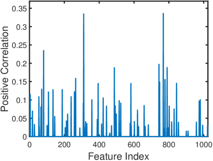
(a) (a) Feed-Forward

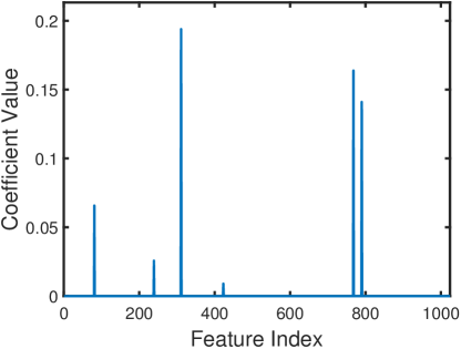
(b) (b) Optimization

(c)

(c)

(d) $\boldsymbol{x}$

(e)

(f) 0.336

$...$

(g)

(h) 0.122

$...$

(i)

(j) 0.083

$...$

(k)

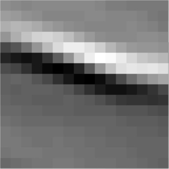
(l) 0.039

$...$

(m)

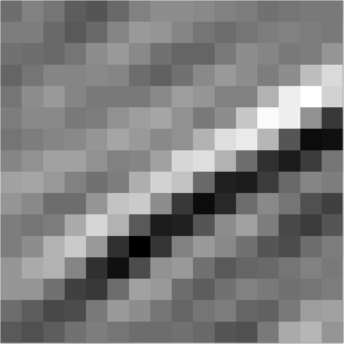
(n) 0.024

$...$

(o)

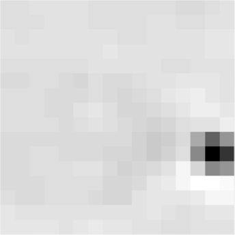
(p) 0.001

(d)

(q)

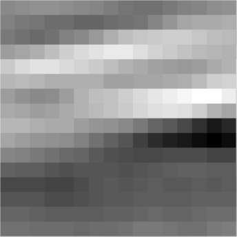
(r) $\hat{\boldsymbol{x}}$

=

(s)

(t) 0.194

+

(u)

(v) 0.164

+

(w)

(x) 0.141

+

(y)

(z) 0.066

+

(aa)

(ab) 0.026

+

(ac)

(ad) 0.009

Figure 1: An example of the “explaining away” conditional dependence provided by optimization-based inference. Sparse representations constructed by feed-forward nonnegative soft thresholding (a) have many more non-zero elements due to redundancy and spurious activations (c). On the other hand, sparse representations found by $\ell_{1}$-penalized, nonnegative least-squares optimization (b) yield a more parsimonious set of components (d) that optimally reconstruct approximations of the data.

Deep convolutional neural networks have achieved remarkable success in the field of computer vision. While far from new [1], the increasing availability of extremely large, labeled datasets along with modern advances in computation with specialized hardware have resulted in state-of-the-art performance in many problems, including essentially all visual learning tasks. Examples include image classification [2], object detection [3], and semantic segmentation [4]. Despite a rich history of practical and theoretical insights about these problems, modern deep learning techniques typically rely on task-agnostic models and poorly-understood heuristics. However, recent work [5, 6, 7] has shown that specialized architectures incorporating classical domain knowledge can increase parameter efficiency, relax training data requirements, and improve performance.

Prior to the advent of modern deep learning, optimization-based methods like component analysis and sparse coding dominated the field of representation learning. These techniques use structured matrix factorization to decompose data into linear combinations of shared components. Latent representations are inferred by minimizing reconstruction error subject to constraints that enforce properties like uniqueness and interpretability. Unlike feed-forward alternatives that construct representations in closed-form via independent feature detectors, this optimization-based approach naturally introduces conditional dependence between features in order to best explain data, a useful phenomenon commonly referred to as “explaining away” within the context of graphical models [8]. An example of this effect is shown in Fig. 1, which compares sparse representations constructed using feed-forward soft thresholding with those given by optimization-based inference with an $\ell_{1}$ penalty. While many components in an overcomplete set of features may have high-correlation with an image, constrained optimization introduces competition between components resulting in more parsimonious representations.

Component analysis methods are also often guided by intuitive goals of incorporating prior knowledge into learned representations. For example, statistical independence allows for the separation of signals into distinct generative sources [9], non-negativity leads to parts-based decompositions of objects [10], and sparsity gives rise to locality and frequency selectivity [11]. Due to the difficulty of enforcing intuitive constraints like these with feed-forward computations, deep learning architectures are instead often motivated by distantly-related biological systems [12] or poorly-understand internal mechanisms such as covariate shift [13] and gradient flow [14]. Furthermore, while a theoretical understanding of deep learning is fundamentally lacking [15], even non-convex formulations of matrix factorization are often associated with guarantees of convergence [16], generalization [17], uniqueness [18], and even global optimality [19].

In order to unify the intuitive and theoretical insights of component analysis with the practical advances made possible through deep learning, we introduce the framework of Deep Component Analysis (DeepCA). This novel model formulation can be interpreted as a multilayer extension of traditional component analysis in which multiple layers are learned jointly with intuitive constraints intended to encode structure and prior knowledge. DeepCA can also be motivated from the perspective of deep neural networks by relaxing the implicit assumption that the input to a layer is constrained to be the output of the previous layer, as shown in Eq. 1 below. In a feed-forward network (left), the output of layer $j$, denoted $\boldsymbol{a}_{j}$, is given in closed-form as a nonlinear function of $\boldsymbol{a}_{j-1}$. DeepCA (right) instead takes a generative approach in which the latent variables $\boldsymbol{w}_{j}$ associated with layer $j$ are inferred to optimally reconstruct $\boldsymbol{w}_{j-1}$ as a linear combination of learned components subject to some constraints $\mathcal{C}_{j}$.

$$\text{Feed-Forward: }\boldsymbol{a}_{j}=\phi(\mathbf{B}_{j}^{\mathsf{T}}\boldsymbol{a}_{j-1})\,\Longrightarrow\,\text{DeepCA: }\mathbf{B}_{j}\boldsymbol{w}_{j}\approx\boldsymbol{w}_{j-1}\text{ s.t. }\boldsymbol{w}_{j}\in\mathcal{C}_{j}$$ (1)

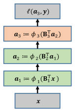
(a) Feed-Forward

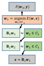
(b) DeepCA

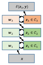
(c) ADNN

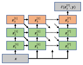
(d) Unrolled ADNN

Figure 2: A comparison between feed-forward neural networks and the proposed deep component analysis (DeepCA) model. While standard deep networks construct learned representations as feed-forward compositions of nonlinear functions (a), DeepCA instead treats them as unknown latent variables to be inferred by constrained optimization (b). To accomplish this, we propose a differentiable inference algorithm that can be expressed as an Alternating Direction Neural Network (ADNN), a recurrent generalization of feed-forward networks (c) that can be unrolled to a fixed number of iterations for learning via backpropagation (d).

From this perspective, intermediate network “activations” cannot be found in closed-form but instead require explicitly solving an optimization problem. While a variety of different techniques could be used for performing this inference, we propose the Alternating Direction Method of Multipliers (ADMM) [20]. Importantly, we demonstrate that after proper initialization, a single iteration of this algorithm is equivalent to a pass through an associated feed-forward neural network with nonlinear activation functions interpreted as proximal operators corresponding to penalties or constraints on the coefficients. The full inference procedure can thus be implemented using Alternating Direction Neural Networks (ADNN), recurrent generalizations of feed-forward networks that allow for parameter learning using backpropagation. A comparison between standard neural networks and DeepCA is shown in Fig. 2. Experimentally, we demonstrate that recurrent passes through convolutional neural networks enable better sparsity control resulting in consistent performance improvements in both supervised and unsupervised tasks without introducing any additional parameters.

More importantly, DeepCA also allows for other constraints that would be impossible to effectively enforce with a single feed-forward pass through a network. As an example, we consider the task of single-image depth prediction, a difficult problem due to the absence of three-dimensional information such as scale and perspective. In many practical scenarios, however, sparse sets of known depth outputs are available for resolving these ambiguities to improve accuracy. This prior knowledge can come from additional sensor modalities like LIDAR or from other 3D reconstruction algorithms that provide sparse depths around textured image regions. Feed-forward networks have been proposed for this problem by concatenating known depth values as an additional input channel [21]. However, while this provides useful context, predictions are not guaranteed to be consistent with the given outputs leading to unrealistic discontinuities. In comparison, DeepCA enforces the constraints by treating predictions as unknown latent variables. Some examples of how this behavior can resolve ambiguities are shown in Fig. 3 where ADNNs with additional iterations learn to propagate information from the given depth values to produce more accurate predictions.

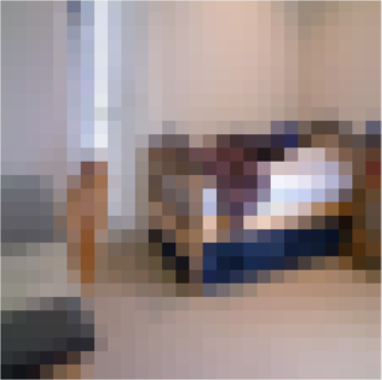
(a)

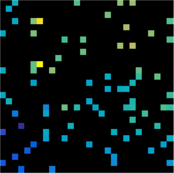
(b)

(c)

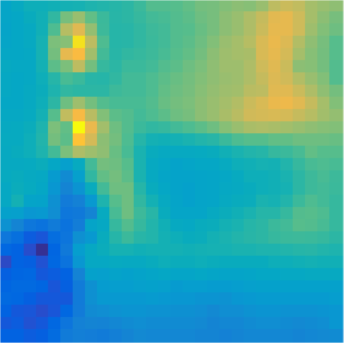
(d)

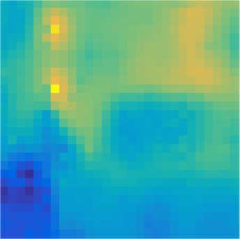
(e)

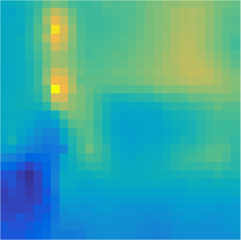
(f)

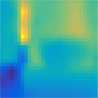
(g)

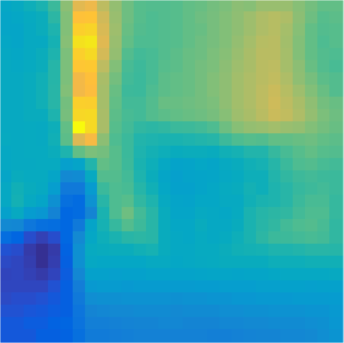
(h)

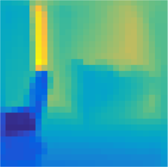
(i)

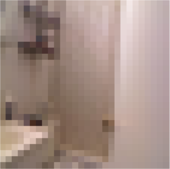
(j)

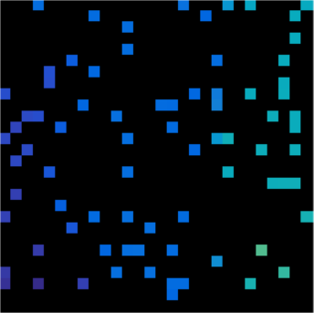
(k)

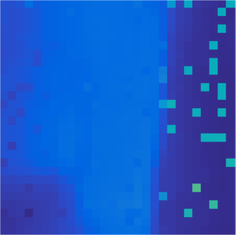
(l)

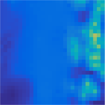
(m)

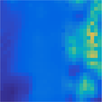
(n)

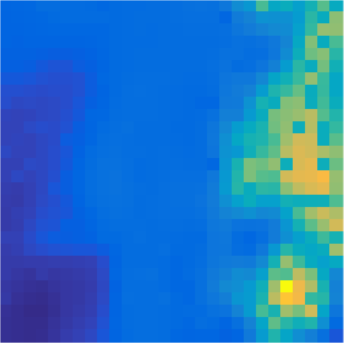
(o)

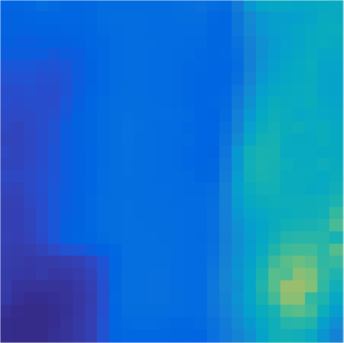
(p)

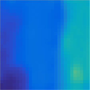
(q)

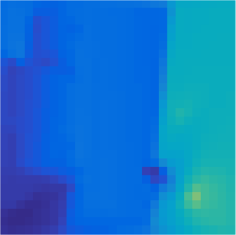
(r)

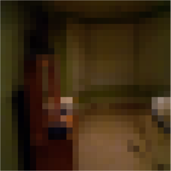
(s)

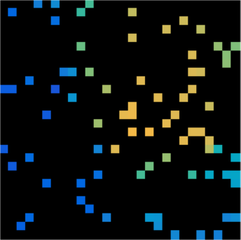
(t)

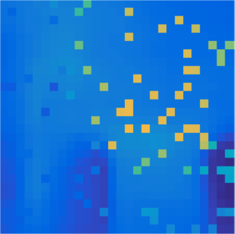
(u)

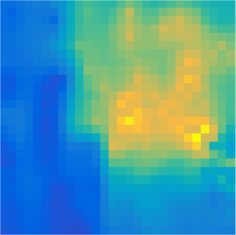
(v)

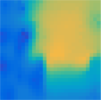
(w)

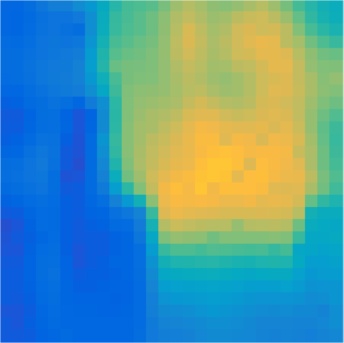
(x)

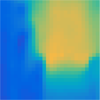
(y)

(z)

(aa)

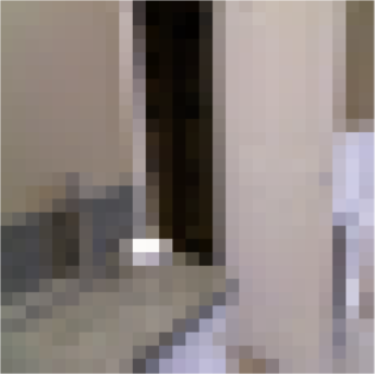
(ab) Image

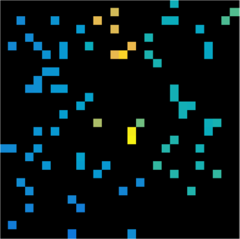
(ac) Given

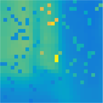
(ad) Baseline

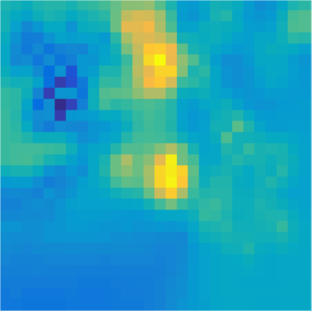
(ae) $\boldsymbol{T=2}$

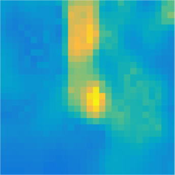
(af) $\boldsymbol{T=3}$

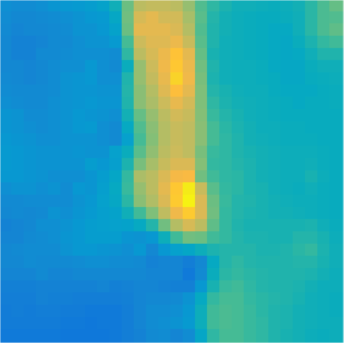
(ag) $\boldsymbol{T=5}$

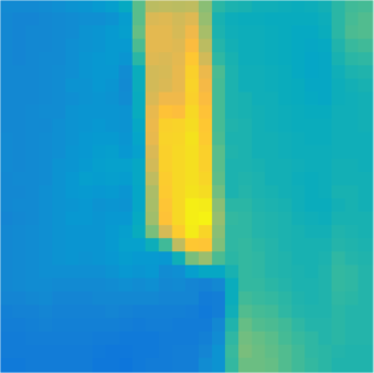
(ah) $\boldsymbol{T=10}$

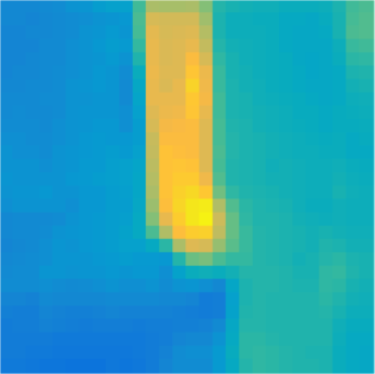
(ai) $\boldsymbol{T=20}$

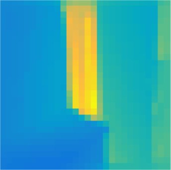
(aj) Truth

Figure 3: A demonstration of DeepCA applied to single-image depth prediction using images concatenated with sparse sets of known depth values as input. Baseline feed-forward networks are not guaranteed to produce outputs that are consistent with the given depth values. ADNNs with an increasing number of iterations ($T>1$) learn to satisfy the sparse output constraints, resolving ambiguities for more accurate predictions without unrealistic discontinuities.

In addition to practical advantages, our model also provides a novel perspective for conceptualizing deep learning techniques. Due to the decoupling of layers provided by relaxing the feed-forward function composition constraints, DeepCA can be equivalently expressed as a shallow model augmented with architecture-dependent structure imposed on the model parameters. In the case of rectified linear unit (ReLU) activation functions [22], this allows for the direct application of results from sparse approximation theory, suggesting new insights towards better understanding why deep neural networks are so effective.

2 Background and Related Work

In order to motivate our approach, we first provide some background on matrix factorization, component analysis, and deep neural networks.

2.1 Component Analysis and Matrix Factorization

Component analysis is a common approach for shallow representation learning that approximately decomposes data $\boldsymbol{x}\in\mathbb{R}^{d}$ into linear combinations of learned components in $\mathbf{B}\in\mathbb{R}^{d\times k}$. This is typically accomplished by minimizing reconstruction error subject to constraints $\mathcal{C}$ on the coefficients that serve to resolve ambiguity or incorporate prior knowledge such as low-rank structure or sparsity. Some examples include Principal Component Analysis (PCA) [23] for dimensionality reduction and sparse dictionary learning [16] which accommodates overcomplete representations by enforcing sparsity.

While component analysis problems are typically non-convex, their structure naturally suggests simple alternating minimization strategies that are often guaranteed to converge [24]. However, unlike backpropagation with stochastic gradient descent, these techniques typically require careful initialization in order to avoid poor local minima. Alternatively, we consider a nested optimization problem that separates learning from inference:

$$\underset{\mathbf{B}}{\arg\min}\sum_{i=1}^{n}\tfrac{1}{2}\lVert\boldsymbol{x}^{(i)}-\mathbf{B}\boldsymbol{f}(\boldsymbol{x}^{(i)})\rVert_{2}^{2}\quad\text{s.t. }\boldsymbol{f}(\boldsymbol{x})=\underset{\boldsymbol{w}\in\mathcal{C}}{\arg\min}\,\tfrac{1}{2}\left\lVert\boldsymbol{x}-\mathbf{B}\boldsymbol{w}\right\rVert_{2}^{2}$$ (2)

Here, the inference function $\boldsymbol{f}:\mathbb{R}^{d}\rightarrow\mathbb{R}^{k}$ is a potentially nonlinear transformation that maps data to their corresponding representations by solving an optimization problem with fixed parameters. For unconstrained PCA with orthogonal components, this inference problem has a simple closed-form solution given by the linear transformation $\boldsymbol{f}^{\mathrm{PCA}}(\boldsymbol{x})=\mathbf{B}^{\mathsf{T}}\boldsymbol{x}$. Substituting this into Eq. 2 results in a linear autoencoder with one hidden layer and tied weights, which has the same unique global minimum but can be trained by backpropagation [25].

With general constraints, inference typically cannot be accomplished in closed form but must instead rely on an iterative optimization algorithm. However, if this algorithm is composed as a finite sequence of differentiable transformations, then the model parameters can still be learned in the same way by backpropagating gradients through the steps of the inference algorithm. We extend this idea by representing an algorithm for inference in our DeepCA model as a recurrent neural network unrolled to a fixed number of iterations.

2.2 Deep Neural Networks

Recently, deep neural networks have emerged as the preferred alternative to component analysis for representation learning of visual data. Their ability to jointly learn multiple layers of abstraction has been shown to allow for encoding increasingly complex features such as textures and object parts [26]. Unlike with component analysis, inference is given in closed-form by design. Specifically, a representation is constructed by passing an image $\boldsymbol{x}$ through the composition of alternating linear transformations with parameters $\mathbf{B}_{j}$ and $\boldsymbol{b}_{j}$ and fixed nonlinear activation functions $\phi_{j}$ for layers $j=1,\dotsc,l$ as follows:

$$\boldsymbol{f}^{\mathrm{DNN}}(\boldsymbol{x})=\phi_{l}\big{(}\mathbf{B}_{l}^{\mathsf{T}}\cdots\phi_{2}(\mathbf{B}_{2}^{\mathsf{T}}(\phi_{1}(\mathbf{B}_{1}^{\mathsf{T}}\boldsymbol{x}-\boldsymbol{b}_{1})-\boldsymbol{b}_{2})\cdots-\boldsymbol{b}_{l}\big{)}$$ (3)

Instead of considering the forward pass of a neural network as an arbitrary nonlinear function, we interpret it as a method for approximate inference in an unsupervised generative model. This follows from previous work which has shown it to be equivalent to bottom-up inference in a probabilistic graphical model [27] or approximate inference in a multi-layer convolutional sparse coding model [28, 29]. However, these approaches have limited practical applicability due to their reliance on careful hyperparameter selection and specialized optimization algorithms. While ADMM has been proposed as a gradient-free alternative to backpropagation for parameter learning [30], we use it only for inference which allows for simpler learning using backpropagation with arbitrary loss functions.

Aside from ADNNs, recurrent feedback has been proposed in other models to improve performance by iteratively refining predictions, especially for applications such as human pose estimation or image segmentation where outputs have complex correlation patterns [31, 32, 33]. While some methods also implement feedback by directly unrolling iterative algorithms, they are often geared towards specific applications such as graphical model inference [34, 35], solving under-determined inverse problems [36, 37, 38], or image alignment [5]. Similar to [39], DeepCA provides a general mechanism for feedback in arbitrary neural networks, but it is motivated by the more interpretable goal of minimizing reconstruction error subject to constraints on network activations.

3 Deep Component Analysis

Deep Component Analysis generalizes the shallow inference objective function in Eq. 2 by introducing additional layers $j=1,\dots,l$ with parameters $\mathbf{B}_{j}\in\mathbb{R}^{p_{j-1}\times p_{j}}$. Optimal DeepCA inference is then accomplished by solving:

$$\boldsymbol{f}^{*}(\boldsymbol{x})=\underset{\{\boldsymbol{w}_{j}\}}{\arg\min}\sum_{j=1}^{l}\tfrac{1}{2}\left\|\boldsymbol{w}_{j-1}-\mathbf{B}_{j}\boldsymbol{w}_{j}\right\|_{2}^{2}+\Phi_{j}(\boldsymbol{w}_{j})\quad\text{s.t. }\boldsymbol{w}_{0}=\boldsymbol{x}$$ (4)

Instead of constraint sets $\mathcal{C}_{j}$, we use penalty functions $\Phi_{j}:\mathbb{R}^{p_{j}}\rightarrow\mathbb{R}$ to enable more general priors. Note that hard constraints can still be represented by indicator functions $I(\boldsymbol{w}_{j}\in\mathcal{C}_{j})$ that equal zero if $\boldsymbol{w}_{j}\in\mathcal{C}_{j}$ and infinity otherwise. While we use pre-multiplication with a weight matrix $\mathbf{B}_{j}$ to simplify notation, our method also supports any linear transformation by replacing transposed weight matrix multiplication with its corresponding adjoint operator. For example, the adjoint of convolution is transposed convolution, a popular approach to upsampling in convolutional networks [40].

If the penalty functions are convex, this problem is also convex and can be solved using standard optimization methods. While this appears to differ substantially from inference in deep neural networks, we later show that it can be seen as a generalization of the feed-forward inference function in Eq. 3. In the remainder of this section, we justify the use of penalty functions in lieu of explicit nonlinear activation functions by drawing connections between non-negative $\ell_{1}$ regularization and ReLU activation functions. We then propose a general algorithm for solving Eq. 4 for the unknown coefficients and formalize the relationship between DeepCA and traditional deep neural networks, which enables parameter learning via backpropagation.

3.1 From Activation Functions to Constraints

Before introducing our inference algorithm, we first discuss the connection between penalties and their nonlinear proximal operators, which forms the basis of the close relationship between DeepCA and traditional neural networks. Ubiquitous within the field of convex optimization, proximal algorithms [41] are methods for solving nonsmooth optimization problems. Essentially, these techniques work by breaking a problem down into a sequence of smaller problems that can often be solved in closed-form by proximal operators $\mathrm{\phi}:\mathbb{R}^{d}\rightarrow\mathbb{R}^{d}$ associated with penalty functions $\Phi:\mathbb{R}^{d}\rightarrow\mathbb{R}$ given by the solution to the following optimization problem, which generalizes projection onto a constraint set:

$$\mathrm{\phi}(\boldsymbol{w})=\underset{\boldsymbol{w}^{\prime}}{\arg\min}\,\tfrac{1}{2}\left\lVert\boldsymbol{w}-\boldsymbol{w}^{\prime}\right\rVert_{2}^{2}+\Phi(\boldsymbol{w}^{\prime})$$ (5)

Within the framework of DeepCA, we interpret nonlinear activation functions in deep networks as proximal operators associated with convex penalties on latent coefficients in each layer. While this connection cannot be used to generalize all nonlinearities, many can naturally be interpreted as proximal operators. For example, the sparsemax activation function is a projection onto the probability simplex [42]. Similarly, the ReLU activation function is a projection onto the nonnegative orthant. When used with a negative bias $\boldsymbol{b}$, it is equivalent to nonnegative soft-thresholding $\mathcal{S}^{+}_{\boldsymbol{b}}$, the proximal operator associated with nonnegative $\mathcal{\ell}_{1}$ regularization:

$$\Phi^{\ell_{1}^{+}}(\boldsymbol{w})=I(\boldsymbol{w}\geq 0)+{\textstyle\sum}_{p}b_{p}\left|w_{p}\right|\quad\Longrightarrow\quad\mathrm{\phi}^{\ell_{1}^{+}}(\boldsymbol{w})=\mathcal{S}^{+}_{\boldsymbol{b}}(\boldsymbol{w})=\mathrm{ReLU}(\boldsymbol{w}-\boldsymbol{b})$$ (6)

While this equivalence has been noted previously as a means to theoretically analyze convolutional neural networks [28], DeepCA supports optimizing the bias $\boldsymbol{b}$ as an $\ell_{1}$ penalty hyperparameter via backpropagation for adaptive regularization, which results in better control of representation sparsity.

In addition to standard activation functions, DeepCA also allows for enforcing additional constraints that encode prior knowledge. For our example of single-image depth prediction with a sparse set of known outputs $\boldsymbol{y}$ provided as prior knowledge, the penalty function on the final output $\boldsymbol{w}_{l}$ is $\boldsymbol{\Phi}_{l}(\boldsymbol{w}_{l})=I(\mathbf{S}\boldsymbol{w}_{l}=\boldsymbol{y})$ where the selector matrix $\mathbf{S}$ extracts the indices corresponding to the known outputs in $\boldsymbol{y}$. The associated proximal operator $\boldsymbol{\phi}_{l}$ projects onto this constraint set by simply correcting the outputs that disagree with the known constraints. Note that this would not be an effective output nonlinearity in a feed-forward network because, while the constraints would be technically satisfied, there is nothing to enforce that they be consistent with neighboring predictions leading to unrealistic discontinuities. In contrast, DeepCA inference minimizes the reconstruction error at each layer subject to these constraints by taking multiple iterations through the network.

3.2 Inference by the Alternating Direction Method of Multipliers

With the model parameters fixed, we solve our DeepCA inference problem using the Alternating Direction Method of Multipliers (ADMM), a general optimization technique that has been successfully used in a wide variety of applications [20]. To derive the algorithm applied to our problem, we first modify our objective function by introducing auxiliary variables $\boldsymbol{z}_{j}$ that we constrain to be equal to the unknown coefficients $\boldsymbol{w}_{j}$, as shown in Eq. 7 below.

$$\underset{\{\boldsymbol{w}_{j},\boldsymbol{z}_{j}\}}{\arg\min}\sum_{j=1}^{l}\tfrac{1}{2}\left\|\boldsymbol{z}_{j-1}{-}\mathbf{B}_{j}\boldsymbol{w}_{j}\right\|_{2}^{2}+\Phi_{j}(\boldsymbol{z}_{j})\quad\text{s.t. }\boldsymbol{w}_{0}=\boldsymbol{x},\,\forall j:\boldsymbol{w}_{j}=\boldsymbol{z}_{j}$$ (7)

From this, we construct the augmented Lagrangian $\mathcal{L}_{\rho}$ with dual variables $\boldsymbol{\lambda}$ and a quadratic penalty hyperparameter $\rho=1$ that can affect convergence speed:

$$\mathcal{L}_{\rho}=\sum_{j=1}^{l}\tfrac{1}{2}\left\|\boldsymbol{z}_{j-1}-\mathbf{B}_{j}\boldsymbol{w}_{j}\right\|_{2}^{2}+\Phi_{j}(\boldsymbol{z}_{j})+\boldsymbol{\lambda}_{j}^{\mathsf{T}}(\boldsymbol{w}_{j}-\boldsymbol{z}_{j})+\tfrac{\rho}{2}\left\lVert\boldsymbol{w}_{j}-\boldsymbol{z}_{j}\right\rVert_{2}^{2}$$ (8)

The ADMM algorithm then proceeds by iteratively minimizing $\mathcal{L}_{\rho}$ with respect to each set of variables with the others fixed, breaking our full inference optimization problem into smaller pieces that can each be solved in closed form. Due to the decoupling of layers in our DeepCA model, the latent activations can be updated incrementally by stepping through each layer in succession, resulting in faster convergence and updates that mirror the computational structure of deep neural networks. With only one layer, our objective function is separable and so this algorithm reduces to the classical two-block ADMM, which has extensive convergence guarantees [20]. For multiple layers, however, this algorithm can be seen as an instance of the cyclical multi-block ADMM with quadratic coupling terms. While our experiments have shown this approach to be effective in our applications, theoretical analysis of its convergence properties is still an active area of research [43].

A single iteration of our algorithm proceeds by taking the following steps for all layers $j=1,\dotsc,l$:

1. First, $\boldsymbol{w}_{j}$ is updated by minimizing the Lagrangian after fixing the associated auxiliary variable $\boldsymbol{z}_{j}$ from the previous iteration along with that of the previous layer $\boldsymbol{z}_{j-1}$ from the current iteration:

   $$\boldsymbol{w}_{j}^{[t+1]} \coloneqq\underset{\boldsymbol{w}_{j}}{\arg\min}\,\mathcal{L}_{\rho}(\boldsymbol{w}_{j},\boldsymbol{z}_{j-1}^{[t+1]},\boldsymbol{z}_{j}^{[t]},\boldsymbol{\lambda}_{j}^{[t]})$$ (9)

   $$=\left(\mathbf{B}_{j}^{\mathsf{T}}\mathbf{B}_{j}+\rho\mathbf{I}\right)^{-1}(\mathbf{B}_{j}^{\mathsf{T}}\boldsymbol{z}_{j-1}^{[t+1]}+\rho\boldsymbol{z}_{j}^{[t]}-\boldsymbol{\lambda}_{j}^{[t]})$$

   The solution to this unconstrained least squares problem is found by solving a linear system of equations.

2. Next, $\boldsymbol{z}_{j}$ is updated by fixing the newly updated $\boldsymbol{w}_{j}$ along with the next layer’s coefficients $\boldsymbol{w}_{j+1}$ from the previous iteration:

   $$\boldsymbol{z}_{j}^{[t+1]} \coloneqq\underset{\boldsymbol{z}_{j}}{\arg\min}\,\mathcal{L}_{\rho}(\boldsymbol{w}_{j}^{[t+1]},\boldsymbol{w}_{j+1}^{[t]},\boldsymbol{z}_{j},\boldsymbol{\lambda}_{j}^{[t]})$$ (10)

   $$=\phi_{j}\big{(}\tfrac{1}{\rho+1}\mathbf{B}_{j+1}\boldsymbol{w}_{j+1}^{[t]}+\tfrac{\rho}{\rho+1}(\boldsymbol{w}_{j}^{[t+1]}+\tfrac{1}{\rho}\boldsymbol{\lambda}_{j}^{[t]})\big{)}$$

   $$\boldsymbol{z}_{l}^{[t+1]} \coloneqq\phi_{j}\big{(}\boldsymbol{w}_{j}^{[t+1]}+\tfrac{1}{\rho}\boldsymbol{\lambda}_{j}^{[t]}\big{)}$$

   This is the proximal minimization problem from Eq. 5, so its solution is given in closed form via the proximal operator $\boldsymbol{\phi}_{j}$ associated with the penalty function $\boldsymbol{\Phi}_{j}$. For $j\neq l$, its argument is a convex combination of the current coefficients $\boldsymbol{w}_{j}$ and feedback that enforces consistency with the next layer.

3. Finally, the dual variables $\boldsymbol{\lambda}_{j}$ are updated with scaled constraint violations.

   $$\boldsymbol{\lambda}_{j}^{[t+1]}\coloneqq\boldsymbol{\lambda}_{j}^{[t]}+\rho(\boldsymbol{w}_{j}^{[t+1]}-\boldsymbol{z}_{j}^{[t+1]})$$ (11)

This process is then repeated until convergence. Though not available as a closed-form expression, in the next section we demonstrate how this algorithm can be posed as a recurrent generalization of a feed-forward neural network.

4 Alternating Direction Neural Networks

Our inference algorithm essentially follows the same pattern as a deep neural network: for each layer, a learned linear transformation is applied to the current output followed by a fixed nonlinear function. Building upon this observation, we implement it using a recurrent network with standard layers, thus allowing the model parameters to be learned using backpropagation.

Recall that the $\boldsymbol{w}_{j}$ update in Eq. 9 requires solving a linear system of equations. While differentiable, this introduces additional computational complexity not present in standard neural networks. To overcome this, we implicitly assume that the parameters in over-complete layers are Parseval tight frames, i.e. so that $\mathbf{B}_{j}\mathbf{B}_{j}^{\mathsf{T}}=\mathbf{I}$. This property is theoretically advantageous in the field of sparse approximation [44] and has been used as a constraint to encourage robustness in deep neural networks [45]. However, in our experiments we found that it was unnecessary to explicitly enforce this assumption during training; with appropriate learning rates, backpropagating through our inference algorithm was enough to ensure that repeated iterations did not result in diverging sequences of variable updates. Thus, under this assumption, we can simplify the update in Eq. 9 using the Woodbury matrix identity as follows:

$$\boldsymbol{w}_{j}^{[t+1]}\coloneqq\tilde{\boldsymbol{z}}_{j}^{[t]}+\tfrac{1}{\rho+1}\mathbf{B}_{j}^{\mathsf{T}}\big{(}\boldsymbol{z}_{j-1}^{[t+1]}-\mathbf{B}_{j}\tilde{\boldsymbol{z}}_{j}^{[t]}\big{)},\quad\tilde{\boldsymbol{z}}_{j}^{[t]}\coloneqq\boldsymbol{z}_{j}^{[t]}-\tfrac{1}{\rho}\boldsymbol{\lambda}_{j}^{[t]}$$ (12)

As this only involves simple linear transformations, our ADMM algorithm for solving the optimization problem in our inference function $\boldsymbol{f}^{*}$ can be expressed as a recurrent neural network that repeatedly iterates until convergence. In practice, however, we unroll the network to a fixed number of iterations $T$ for an approximation of optimal inference so that $\boldsymbol{f}^{[T]}(\boldsymbol{x})\approx\boldsymbol{f}^{*}(\boldsymbol{x})$. Our full algorithm is summarized in Algs. 4 and 4.

Algorithm 1:  Feed-Forward

Input: $\boldsymbol{x}$, $\{\mathbf{B}_{j},\boldsymbol{b}_{j}\}$

Output: $\{\boldsymbol{w}_{j}\}$, $\{\boldsymbol{z}_{j}\}$

Initialize: $\boldsymbol{z}_{0}=\boldsymbol{x}$

for $j=1,\dotsc,l$ do

       Pre-activation:

       $\boldsymbol{w}_{j}\coloneqq\mathbf{B}_{j}^{\mathsf{T}}\boldsymbol{z}_{j-1}$

      Activation:

       $\boldsymbol{z}_{j}\coloneqq\phi_{j}(\boldsymbol{w}_{j}-\boldsymbol{b}_{j})$

end for

Algorithm 2:  Alternating Direction Neural Network

Input: $\boldsymbol{x}$, $\{\mathbf{B}_{j},\boldsymbol{b}_{j}\}$

Output: $\{\boldsymbol{w}_{j}^{[T]}\}$, $\{\boldsymbol{z}_{j}^{[T]}\}$

Initialize: $\{\boldsymbol{\lambda}_{j}^{[0]}\}=\boldsymbol{0}$, $\{\boldsymbol{w}^{[1]}_{j},\boldsymbol{z}^{[1]}_{j}\}$ from Alg. 4

for $t=1,\dotsc,T-1$ do

       for $j=1,\dotsc,l$ do

             Dual: Update $\boldsymbol{\lambda}_{j}^{[t]}$ (Eq. 11)

            Pre-activation: Update $\boldsymbol{w}_{j}^{[t+1]}$ (Eq. 12)

            Activation: Update $\boldsymbol{z}_{j}^{[t+1]}$ (Eq. 10)

       end for

      

end for

4.1 Generalization of Feed-Forward Networks

Given proper initialization of the variables, a single iteration of this algorithm is identical to a pass through a feed-forward network. Specifically, if we let $\boldsymbol{\lambda}_{j}^{[0]}=\boldsymbol{0}$ and $\boldsymbol{z}_{j}^{[0]}=\mathbf{B}_{j}^{\mathsf{T}}\boldsymbol{z}_{j-1}^{[1]}$, where we again denote $\boldsymbol{z}_{0}^{[1]}=\boldsymbol{x}$, then $\boldsymbol{w}_{j}^{[1]}$ is equivalent to the pre-activation of a neural network layer:

$$\boldsymbol{w}_{j}^{[1]}\coloneqq\boldsymbol{z}_{j}^{[0]}+\tfrac{1}{\rho+1}\mathbf{B}_{j}^{\mathsf{T}}\big{(}\boldsymbol{z}_{j-1}^{[1]}-\mathbf{B}_{j}(\mathbf{B}_{j}^{\mathsf{T}}\boldsymbol{z}_{j-1}^{[1]})\big{)}=\mathbf{B}_{j}^{\mathsf{T}}\boldsymbol{z}_{j-1}^{[1]}$$ (13)

Similarly, if we initialize $\boldsymbol{w}_{j+1}^{[0]}=\mathbf{B}_{j+1}^{\mathsf{T}}\boldsymbol{w}_{j}^{[1]}$, then $\boldsymbol{z}_{j}^{[1]}$ is equivalent to the corresponding nonlinear activation using the proximal operator $\phi_{j}$:

$$\boldsymbol{z}_{j}^{[1]}\coloneqq\phi_{j}\big{(}\tfrac{1}{\rho+1}\mathbf{B}_{j+1}(\mathbf{B}_{j+1}^{\mathsf{T}}\boldsymbol{w}_{j}^{[1]})+\tfrac{\rho}{\rho+1}\boldsymbol{w}_{j}^{[1]}\big{)}=\phi_{j}\big{(}\boldsymbol{w}_{j}^{[1]}\big{)}$$ (14)

Thus, one iteration of our inference algorithm is equivalent to the standard feed-forward neural network given in Eq. 3, i.e. $\boldsymbol{f}^{[1]}(\boldsymbol{x})=\boldsymbol{f}^{\mathrm{DNN}}(\boldsymbol{x})$, where nonlinear activation functions are interpreted as proximal operators corresponding to the penalties of our DeepCA model. Additional iterations through the network lead to more accurate inference approximations while explicitly satisfying constraints on the latent variables.

4.2 Learning by Backpropagation

With DeepCA inference approximated by differentiable ADNNs, the model parameters can be learned in the same way as standard feed-forward networks. Extending the nested component analysis optimization problem from Eq. 2, the inference function $\boldsymbol{f}^{[T]}$ can be used as a generalization of feed-forward network inference $\boldsymbol{f}^{[1]}$ for backpropagation with arbitrary loss functions $L$ that encourage the output to be consistent with provided supervision $\boldsymbol{y}^{(i)}$, as shown in Eq. 15 below. Here, only the latent coefficients $\boldsymbol{f}_{l}^{[T]}(\boldsymbol{x}^{(i)})$ from the last layer are shown in the loss function, but other intermediate outputs $j\neq l$ could also be included.

$$\underset{\{\mathbf{B}_{j},\boldsymbol{b}_{j}\}}{\arg\min}\sum_{i=1}^{n}L\big{(}\boldsymbol{f}_{l}^{[T]}(\boldsymbol{x}^{(i)}),\,\boldsymbol{y}^{(i)}\big{)}$$ (15)

From an agnostic perspective, an ADNN can thus be seen as an end-to-end deep network architecture with a particular sequence of linear and nonlinear transformations and tied weights. More iterations ($T>1$) result in networks with greater effective depth, potentially allowing for the representation of more complex nonlinearities. However, because the network architecture was derived from an algorithm for inference in our DeepCA model instead of arbitrary compositions of parameterized transformations, the greater depth requires no additional parameters and serves the very specific purpose of satisfying constraints on the latent variables while enforcing consistency with the model parameters.

4.3 Theoretical Insights

In addition to the practical advantages of recurrent ADNNs for constraint satisfaction, our DeepCA model provides a useful theoretical tool for better understanding traditional neural networks. In prior work, Papyan et al. analyzed feed-forward networks as a method for approximate inference in a multilayer convolutional sparse coding model [28], which can be seen as a special case of DeepCA with overcomplete dictionaries and fixed constraints on the sparsity of the coefficients subject to exact reconstructions in each layer. Specifically, they provide conditions under which the activations of a feed-forward convolutional network with ReLU nonlinearities approximate the true coefficients of their model with bounded error and exact support recovery. While these conditions are likely too strict to be satisfied in practice (see Fig. 1, for example), the theoretical connection emphasizes the importance of sparsity and demonstrates the potential for analyzing deep neural networks from the perspective of sparse approximation theory.

Our more general DeepCA model introduces penalties that relax the requirement of exact reconstruction at each layer, effectively introducing errors that break up the standard compositional structure of neural networks. Importantly, this decoupling of layers allows our original multilayer inference function in Eq. 4 to be expressed as the equivalent shallow learning problem:

$$\boldsymbol{f}^{*}(\boldsymbol{x})=\underset{\{\boldsymbol{w}_{j}\}}{\arg\min}\,\frac{1}{2}\left\lVert\left[\begin{array}[]{c}\boldsymbol{x}\\ \mathbf{0}\\[-3.00003pt] \vdots\\ \mathbf{0}\end{array}\right]-\left[\begin{array}[]{cccc}\mathbf{B}_{1}&\mathbf{0}&&\mathbf{0}\\[-6.00006pt] -\mathbf{I}&\mathbf{B}_{2}&\ddots\\[-5.0pt] &\ddots&\ddots&\mathbf{0}\\[-1.00006pt] \mathbf{0}&&-\mathbf{I}&\mathbf{B}_{l}\end{array}\right]\left[\begin{array}[]{c}\boldsymbol{w}_{1}\\ \boldsymbol{w}_{2}\\[-1.99997pt] \vdots\\[-1.99997pt] \boldsymbol{w}_{l}\end{array}\right]\right\rVert_{2}^{2}+\sum_{j=1}^{l}\Phi_{j}(\boldsymbol{w}_{j})$$ (16)

With nonnegative $\ell_{1}$ penalties corresponding to biased ReLU activation functions, this is simply an augmented, higher-dimensional nonnegative sparse coding problem in which the dictionary is constrained to have a particular block structure that relates to the architecture of the corresponding neural network. This suggests that nonlinear function composition may not be necessary for effective deep learning, but instead the implicit structure that it enforces.

This connection to shallow learning allows for the direct application of results from the field of sparse approximation theory. For example, despite being able to exactly reconstruct any datapoint, if overcomplete dictionaries satisfy certain incoherence properties, then the sparsest set of reconstruction coefficients may actually be unique [46]. Uniqueness is an important characteristic of learned representations that are able to memorize data, a prominent feature in many effective deep architectures [47]. While standard shallow models are typically incapable of satisfying the properties required for uniqueness in high-dimensional datasets like those common in the field of computer vision, DeepCA suggests that the increased capacity of deep networks can be explained by the structure imposed on the augmented dictionaries of Eq. 16. Higher-dimensionality allows for richer unique representations with a greater number of non-zero elements while the block structure reduces the number of free parameters that need to be learned. Uniqueness guarantees can also apply to solutions of sparse nonnegative least squares problems even without explicitly enforcing sparsity [48], which may help to explain the success of deep networks without explicit bias terms [2]. More broadly, we believe that DeepCA opens up a fruitful new direction for future research towards the principled design of neural network architectures that optimize capacity for sparse representation by enforcing implicit structure on the augmented dictionaries of their associated shallow models.

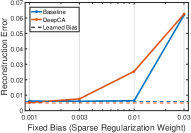
(a) Decoder Error

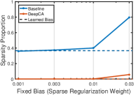
(b) Layer 1 Sparsity

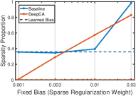
(c) Layer 2 Sparsity

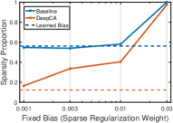
(d) Layer 3 Sparsity

 

Figure 4: A demonstration of the effects of fixed (solid lines) and learnable (dotted lines) bias parameters on the reconstruction error (a) and activation sparsity (b-d) comparing feed forward networks (blue) with DeepCA (red). All models consist of three layers each with 512 components. Due to the conditional dependence provided by recurrent feedback, DeepCA learns to better control the sparsity level in order improve reconstruction error. As $\ell_{1}$ regularization weights, the biases converge towards zero resulting in denser activations and higher network capacity for reconstruction.

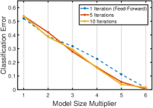
(a) Training Error

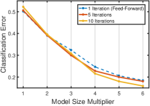
(b) Testing Error

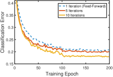
(c) Optimization

Figure 5: The effect of increasing model size on training (a) and testing (b) classification error, demonstrating consistently improved performance of ADNNs over feed-forward networks, especially in larger models. The base model consists of two $3\times 3$, 2-strided convolutional layers followed by one fully-connected layer with 4, 8, and 16 components respectively. Also shown are is the classification error throughout training (c).

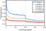
(a) Training

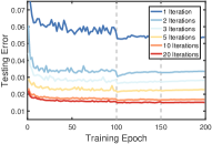
(b) Testing

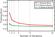
(c) Train Error

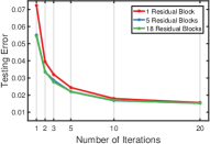
(d) Test Error

 

Figure 6: Quantitative results demonstrating the improved generalization performance of ADNN inference. The training (a) and testing (b) reconstruction errors throughout optimization show that more iterations ($T>1$) substantially reduce convergence time and give much lower error on held-out test data. With a sufficiently large number of iterations, even lower-capacity models with encoders consisting of fewer residual blocks all achieve nearly the same level of performance with small discrepancies between training (c) and testing (d) errors.

(a) Input Image

(a)

(b)

(c)

(d)

(e)

(f)

(g)

(h)

(i)

(j)

(b) Baseline ($T=1$)

(k)

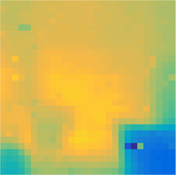
(l)

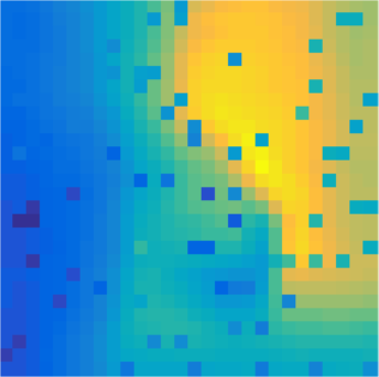
(m)

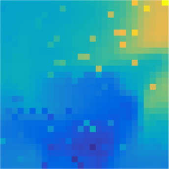
(n)

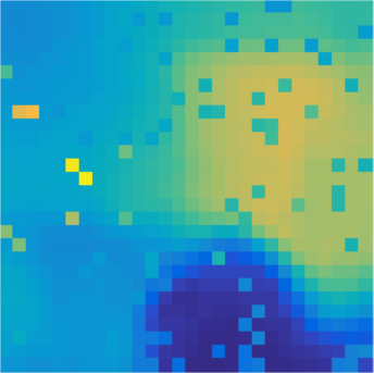
(o)

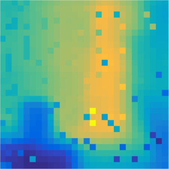
(p)

(q)

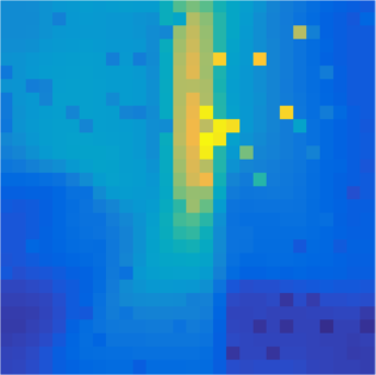
(r)

(s)

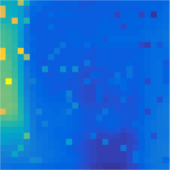
(t)

(c) ADNN ($\boldsymbol{T=20}$)

(u)

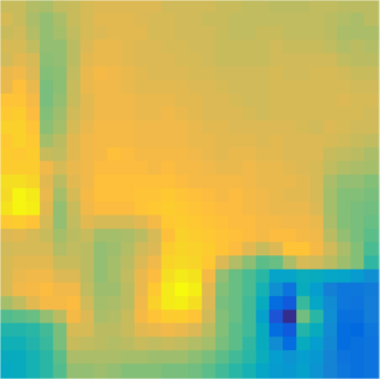
(v)

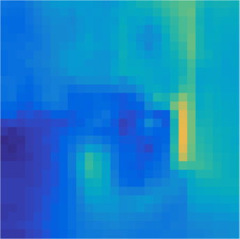
(w)

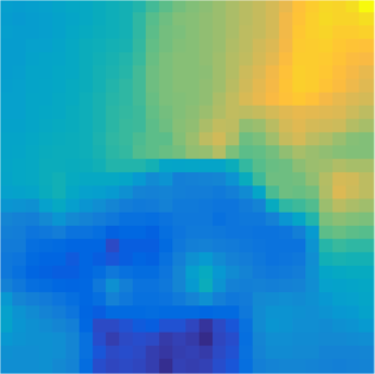
(x)

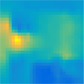
(y)

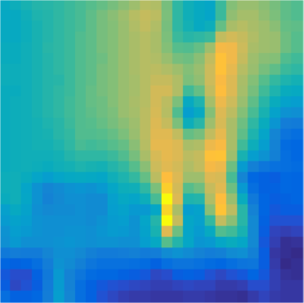
(z)

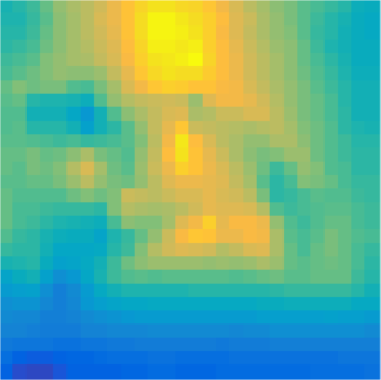
(aa)

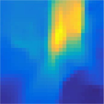
(ab)

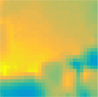
(ac)

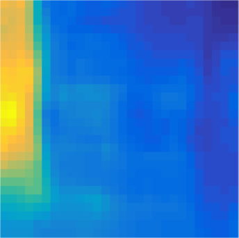
(ad)

(d) Ground Truth

(ae)

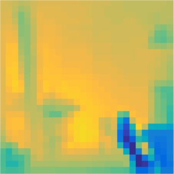
(af) (i)

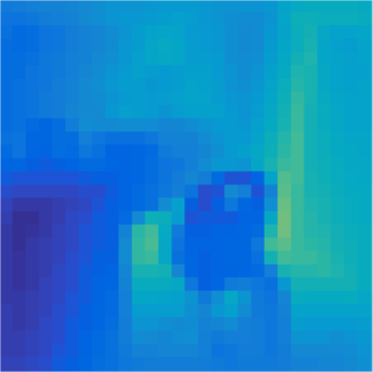
(ag) (ii)

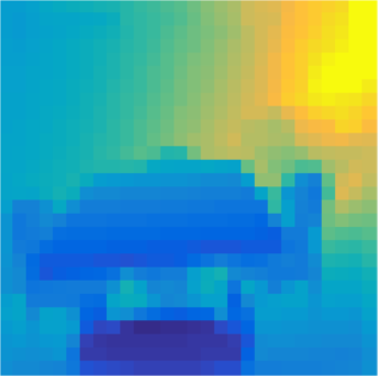
(ah) (iii)

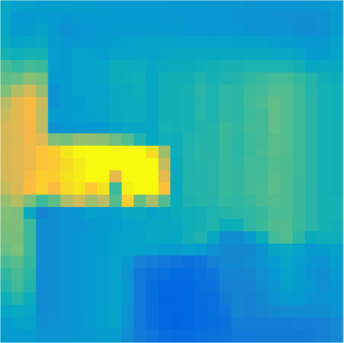
(ai) (iv)

(aj) (v)

(ak) (vi)

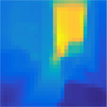
(al) (vii)

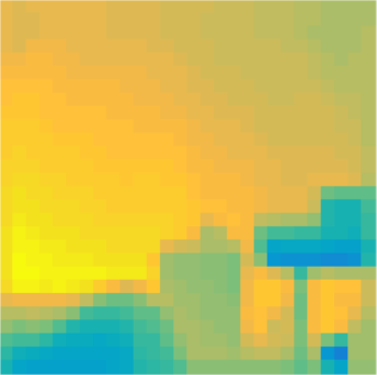
(am) (viii)

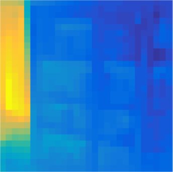
(an) (ix)

(a) Input Image

(ao)

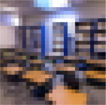
(ap)

(aq)

(ar)

(as)

(at)

(au)

(av)

(aw)

(ax)

(b) Baseline ($T=1$)

(ay)

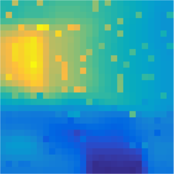
(az)

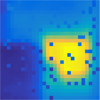
(ba)

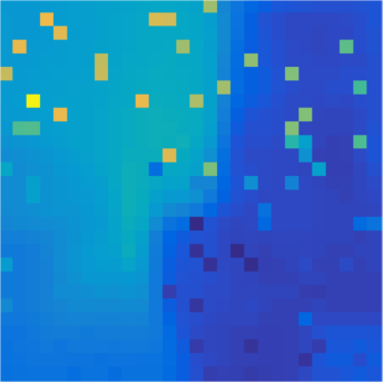
(bb)

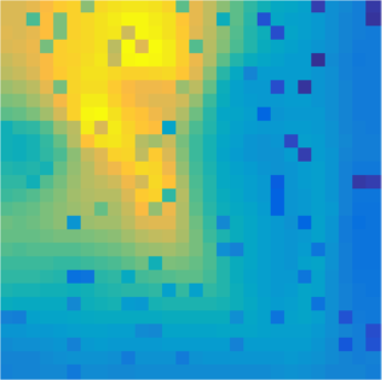
(bc)

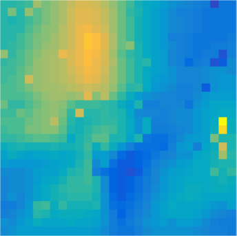
(bd)

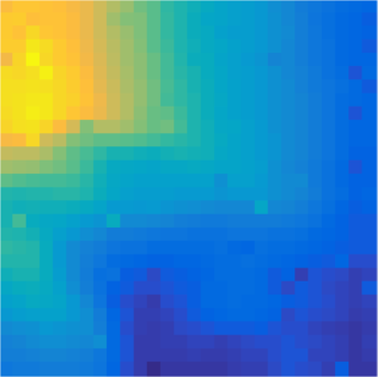
(be)

(bf)

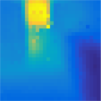
(bg)

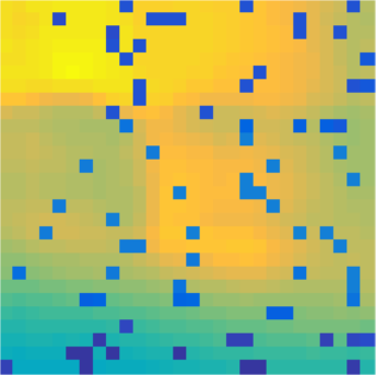
(bh)

(c) ADNN ($\boldsymbol{T=20}$)

(bi)

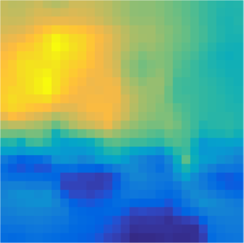
(bj)

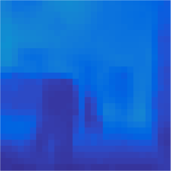
(bk)

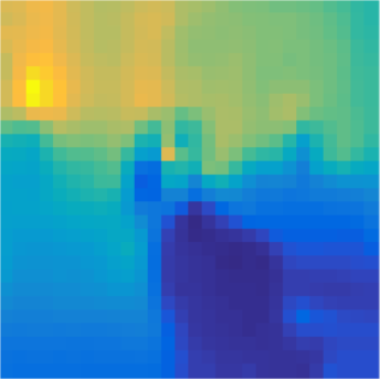
(bl)

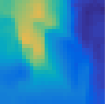
(bm)

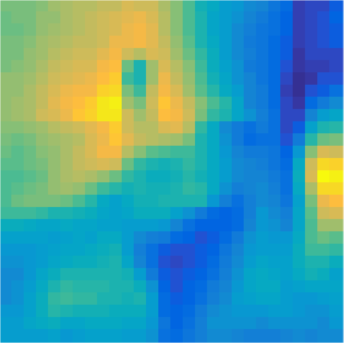
(bn)

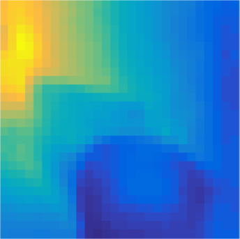
(bo)

(bp)

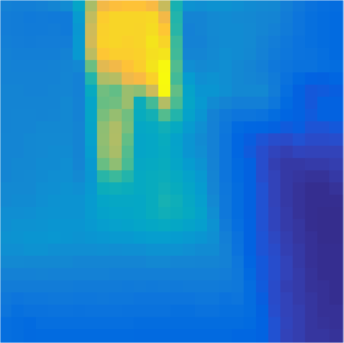
(bq)

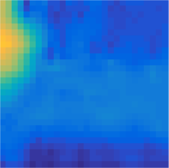
(br)

(d) Ground Truth

(bs)

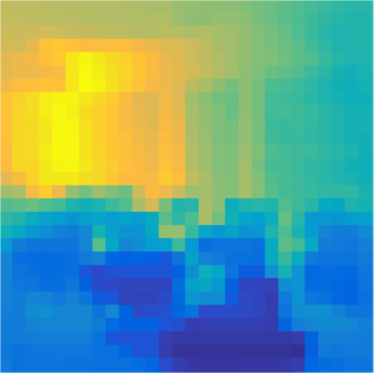
(bt) (x)

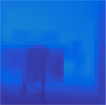
(bu) (xi)

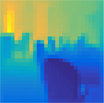
(bv) (xii)

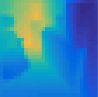
(bw) (xiii)

(bx) (xiv)

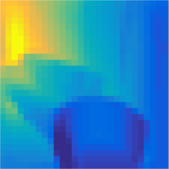
(by) (xv)

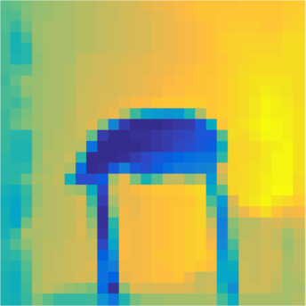
(bz) (xvi)

(ca) (xvii)

(cb) (xviii)

Figure 7: Qualitative depth prediction results given a single image (a) and a sparse set of known depth values as input. Outputs of the baseline feed-forward model (b) are inconsistent with the constraints as evidenced by unrealistic discontinuities. An ADNN with $T=20$ iterations (c) learns to enforce the constraints, resolving ambiguities for more detailed predictions that better agree with ground truth depth maps (d). Depending on the difficulty, additional iterations may have little effect on the output (xvii) or be insufficient to consistently integrate the known constraint values (xviii).

5 Experimental Results

In this section, we demonstrate some practical advantages of more accurate inference approximations in our DeepCA model using recurrent ADNNs over feed-forward networks. Even without additional prior knowledge, standard convolutional networks with ReLU activation functions still benefit from additional recurrent iterations as demonstrated by consistent improvements in both supervised and unsupervised tasks on the CIFAR-10 dataset [49]. Specifically, with an unsupervised $\ell_{2}$ reconstruction loss function, Fig. 4 shows that the conditional dependence between features provided by additional iterations allows for better sparsity control, resulting in higher network capacity through denser activations and lower reconstruction error. This suggests that recurrent feedback allows ADNNs to learn richer representation spaces by explicitly penalizing activation sparsity. With a supervised classification loss function, backpropagating through inference allows biases to be used for adaptive regularization, providing more freedom in modulating activation sparsity to increase model capacity by ensuring the uniqueness of representations across semantic categories. This results in improved classification performance as shown in Fig. 5, especially for wider models with more components per layer.

While these experiments emphasize the importance of sparsity in deep networks and justify our DeepCA model formulation, the effectiveness of feed-forward soft thresholding as an approximation of explicit $\ell_{1}$ regularization limits the amount of additional capacity that can be achieved with more iterations. As such, ADNNs provide much greater performance gains when prior knowledge is available in the form of constraints that cannot be effectively approximated by feed-forward nonlinearities. This is exemplified by our application of output-constrained single-image depth prediction where simple feed-forward correction of the known depth values results in inconsistent discontinuities. We demonstrate this with the NYU-Depth V2 dataset [50], from which we sample 60k training images and 500 testing images from held-out scenes. To facilitate faster training, we resize the images to $28\times 28$ and then randomly sample 10% of the ground truth depth values to simulate known measurements. Following [21], our model architecture uses a ResNet encoder for feature extraction of the image concatenated with the known depth values as an additional input channel. This is followed by an ADNN decoder composed of three transposed convolution upsampling layers with biased ReLU nonlinearites in the first two layers and a constraint correction proximal operator in the last layer. Fig. 6 shows the mean absolute prediction errors of this model with increasing numbers of iterations and different encoder sizes. While all models have similar prediction error on training data, ADNNs with more iterations achieve significantly improved generalization performance, reducing the test error of the feed-forward baseline by over 72% from 0.054 to 0.015 with 20 iterations even with low-capacity encoders. Qualitative visualizations in Fig. 7 show that these improvements result from consistent constraint satisfaction that serves to resolve depth ambiguities.

6 Conclusion

DeepCA is a novel deep model formulation that extends shallow component analysis techniques to increase representational capacity. Unlike feed-forward networks, intermediate network activations are interpreted as latent reconstruction coefficients to be inferred using an iterative constrained optimization algorithm. This is implemented using recurrent ADNNs, which allow the model parameters to be learned with arbitrary loss functions. In addition, they provide a tool for consistently integrating prior knowledge in the form of constraints or regularization penalties. Due to its close relationship to feed-forward networks, which are equivalent to one iteration of this algorithm with proximal operators replacing nonlinear activation functions, DeepCA also provides a novel theoretical perspective from which to interpret deep networks. This suggests the use of sparse approximation theory as tool for analyzing and designing network architectures that optimize the capacity for learning unique representations of data.

References

- [1] LeCun, Y., Bottou, L., Bengio, Y., Haffner, P.: Gradient-based learning applied to document recognition. Proceedings of the IEEE 86(11) (1998) 2278–2324
- [2] Huang, G., Liu, Z., Weinberger, K.Q., van der Maaten, L.: Densely connected convolutional networks. In: Conference on Computer Vision and Pattern Recognition (CVPR). (2017)
- [3] Huang, J., Rathod, V., Sun, C., Zhu, M., Korattikara, A., Fathi, A., Fischer, I., Wojna, Z., Song, Y., Guadarrama, S., Murphy, K.: Speed/accuracy trade-offs for modern convolutional object detectors. In: Conference on Computer Vision and Pattern Recognition (CVPR). (2017)
- [4] Chen, L.C., Papandreou, G., Kokkinos, I., Murphy, K., Yuille, A.L.: DeepLab: Semantic image segmentation with deep convolutional nets, atrous convolution, and fully connected CRFs. Pattern Analysis and Machine Intelligence (PAMI) PP(99) (2017)
- [5] Lin, C.H., Lucey, S.: Inverse compositional spatial transformer networks. Conference on Computer Vision and Pattern Recognition (CVPR) (2017)
- [6] Tulsiani, S., Zhou, T., Efros, A.A., Malik, J.: Multi-view supervision for single-view reconstruction via differentiable ray consistency. In: Conference on Computer Vision and Pattern Recognition (CVPR). (2017)
- [7] Brachmann, E., Krull, A., Nowozin, S., Shotton, J., Michel, F., Gumhold, S., Rother, C.: Dsac-differentiable ransac for camera localization. In: Conference on Computer Vision and Pattern Recognition (CVPR). (2017)
- [8] Bengio, Y., Courville, A., Vincent, P.: Representation learning: A review and new perspectives. Pattern Analysis and Machine Intelligence (PAMI) 35(8) (2013) 1798–1828
- [9] Jutten, C., Herault, J.: Blind separation of sources, part i: An adaptive algorithm based on neuromimetic architecture. Signal Processing 24(1) (1991) 1–10
- [10] Lee, D.D., Seung, H.S.: Learning the parts of objects by non-negative matrix factorization. Nature 401(6755) (1999) 788–791
- [11] Olshausen, B.A., et al.: Emergence of simple-cell receptive field properties by learning a sparse code for natural images. Nature 381(6583) (1996) 607–609
- [12] Simonyan, K., Zisserman, A.: Two-stream convolutional networks for action recognition in videos. In: Advances in Neural Information Processing Systems (NIPS). (2014)
- [13] Ioffe, S., Szegedy, C.: Batch normalization: Accelerating deep network training by reducing internal covariate shift. In: International Conference on Machine Learning (ICML). (2015) 448–456
- [14] He, K., Zhang, X., Ren, S., Sun, J.: Identity mappings in deep residual networks. In: European Conference on Computer Vision (ECCV). (2016)
- [15] Zhang, C., Bengio, S., Hardt, M., Recht, B., Vinyals, O.: Understanding deep learning requires rethinking generalization. In: International Conference on Learning Representations (ICLR). (2017)
- [16] Bao, C., Ji, H., Quan, Y., Shen, Z.: Dictionary learning for sparse coding: Algorithms and convergence analysis. Pattern Analysis and Machine Intelligence (PAMI) 38(7) (2016) 1356–1369
- [17] Liu, T., Tao, D., Xu, D.: Dimensionality-dependent generalization bounds for k-dimensional coding schemes. Neural computation (2016)
- [18] Gillis, N.: Sparse and unique nonnegative matrix factorization through data preprocessing. Journal of Machine Learning Research (JMLR) 13(November) (2012) 3349–3386
- [19] Haeffele, B., Young, E., Vidal, R.: Structured low-rank matrix factorization: Optimality, algorithm, and applications to image processing. In: International Conference on Machine Learning (ICML). (2014)
- [20] Boyd, S., Parikh, N., Chu, E., Peleato, B., Eckstein, J.: Distributed optimization and statistical learning via the alternating direction method of multipliers. Foundations and Trends® in Machine Learning 3(1) (2011)
- [21] Ma, F., Karaman, S.: Sparse-to-dense: Depth prediction from sparse depth samples and a single image. In: International Conference on Robotics and Automation (ICRA). (2018)
- [22] Glorot, X., Bordes, A., Bengio, Y.: Deep sparse rectifier neural networks. In: International Conference on Artificial Intelligence and Statistics (AISTATS). (2011)
- [23] Wold, S., Esbensen, K., Geladi, P.: Principal component analysis. Chemometrics and intelligent laboratory systems 2(1-3) (1987) 37–52
- [24] Xu, Y., Yin, W.: A block coordinate descent method for regularized multiconvex optimization with applications to nonnegative tensor factorization and completion. SIAM Journal on imaging sciences 6(3) (2013) 1758–1789
- [25] Baldi, P., Hornik, K.: Neural networks and principal component analysis: Learning from examples without local minima. Neural networks 2(1) (1989) 53–58
- [26] Lee, H., Grosse, R., Ranganath, R., Ng, A.Y.: Convolutional deep belief networks for scalable unsupervised learning of hierarchical representations. In: International Conference on Machine Learning (ICML). (2009)
- [27] Patel, A.B., Nguyen, M.T., Baraniuk, R.: A probabilistic framework for deep learning. In: Advances in Neural Information Processing Systems (NIPS). (2016)
- [28] Papyan, V., Romano, Y., Elad, M.: Convolutional neural networks analyzed via convolutional sparse coding. Journal of Machine Learning Research (JMLR) 18(83) (2017)
- [29] Sulam, J., Papyan, V., Romano, Y., Elad, M.: Multi-layer convolutional sparse modeling: Pursuit and dictionary learning. arXiv preprint arXiv:1708.08705 (2017)
- [30] Taylor, G., Burmeister, R., Xu, Z., Singh, B., Patel, A., Goldstein, T.: Training neural networks without gradients: A scalable admm approach. In: International Conference on Machine Learning (ICML). (2016)
- [31] Carreira, J., Agrawal, P., Fragkiadaki, K., Malik, J.: Human pose estimation with iterative error feedback. In: Conference on Computer Vision and Pattern Recognition (CVPR). (2016)
- [32] Belagiannis, V., Zisserman, A.: Recurrent human pose estimation. In: International Conference on Automatic Face & Gesture Recognition (FG). (2017)
- [33] Li, K., Hariharan, B., Malik, J.: Iterative instance segmentation. In: Conference on Computer Vision and Pattern Recognition (CVPR). (2016)
- [34] Chen, L.C., Schwing, A., Yuille, A., Urtasun, R.: Learning deep structured models. In: International Conference on Machine Learning (ICML). (2015)
- [35] Hu, P., Ramanan, D.: Bottom-up and top-down reasoning with hierarchical rectified gaussians. In: Conference on Computer Vision and Pattern Recognition (CVPR). (2016)
- [36] Gregor, K., LeCun, Y.: Learning fast approximations of sparse coding. In: International Conference on Machine Learning (ICML). (2010)
- [37] Diamond, S., Sitzmann, V., Heide, F., Wetzstein, G.: Unrolled optimization with deep priors. arXiv preprint arXiv:1705.08041 (2017)
- [38] Sun, J., Li, H., Xu, Z., et al.: Deep admm-net for compressive sensing mri. In: Advances in Neural Information Processing Systems (NIPS). (2016)
- [39] Zamir, A.R., Wu, T.L., Sun, L., Shen, W., Malik, J., Savarese, S.: Feedback networks. In: Advances in Neural Information Processing Systems (NIPS). (2017)
- [40] Noh, H., Hong, S., Han, B.: Learning deconvolution network for semantic segmentation. In: International Conference on Computer Vision (ICCV). (2015)
- [41] Parikh, N., Boyd, S., et al.: Proximal algorithms. Foundations and Trends® in Optimization 1(3) (2014)
- [42] Martins, A., Astudillo, R.: From softmax to sparsemax: A sparse model of attention and multi-label classification. In: International Conference on Machine Learning (ICML). (2016)
- [43] Chen, C., Li, M., Liu, X., Ye, Y.: Extended admm and bcd for nonseparable convex minimization models with quadratic coupling terms: convergence analysis and insights. Mathematical Programming (2017)
- [44] Casazza, P.G., Kutyniok, G.: Finite frames: Theory and applications. Springer (2012)
- [45] Moustapha, C., Piotr, B., Edouard, G., Yann, D., Nicolas, U.: Parseval networks: Improving robustness to adversarial examples. arXiv preprint arXiv:1704.08847 (2017)
- [46] Donoho, D.L., Elad, M.: Optimally sparse representation in general (nonorthogonal) dictionaries via ℓ1 minimization. Proceedings of the National Academy of Sciences 100(5) (2003) 2197–2202
- [47] Arpit, D., Jastrzebski, S., Ballas, N., Krueger, D., Bengio, E., Kanwal, M.S., Maharaj, T., Fischer, A., Courville, A., Bengio, Y., Lacoste-Julien, S.: A closer look at memorization in deep networks. In: International Conference on Machine Learning (ICML). (2017) 233–242
- [48] Bruckstein, A.M., Elad, M., Zibulevsky, M.: On the uniqueness of nonnegative sparse solutions to underdetermined systems of equations. IEEE Transactions on Information Theory 54(11) (2008) 4813–4820
- [49] Krizhevsky, A., Hinton, G.: Learning multiple layers of features from tiny images. Technical report, University of Toronto (2009)
- [50] Nathan Silberman, Derek Hoiem, P.K., Fergus, R.: Indoor segmentation and support inference from rgbd images. In: European Conference on Computer Vision (ECCV). (2012)