Improving the efficiency and robustness of nested sampling using posterior repartitioning

Abstract

In real-world Bayesian inference applications, prior assumptions regarding the parameters of interest may be unrepresentative of their actual values for a given dataset. In particular, if the likelihood is concentrated far out in the wings of the assumed prior distribution, this can lead to extremely inefficient exploration of the resulting posterior by nested sampling (NS) algorithms, with unnecessarily high associated computational costs. Simple solutions such as broadening the prior range in such cases might not be appropriate or possible in real-world applications, for example when one wishes to assume a single standardised prior across the analysis of a large number of datasets for which the true values of the parameters of interest may vary. This work therefore introduces a posterior repartitioning (PR) method for NS algorithms, which addresses the problem by redefining the likelihood and prior while keeping their product fixed, so that the posterior inferences and evidence estimates remain unchanged but the efficiency of the NS process is significantly increased. Numerical results show that the PR method provides a simple yet powerful refinement for NS algorithms to address the issue of unrepresentative priors.

1 Introduction

Bayesian inference (see e.g. MacKay 2003) provides a comprehensive framework for estimating unknown parameter(s) $\mathbf{\mathit{\theta}}$ of some model with the assistance both of observed data $\mathcal{D}$ and prior knowledge of $\mathbf{\mathit{\theta}}$. One is interested in obtaining the posterior distribution of $\mathbf{\mathit{\theta}}$, and this can be expressed using Bayes’ theorem as:

$$\Pr(\mathbf{\mathit{\theta}}|\mathcal{D},\mathcal{M})=\frac{\Pr(\mathcal{D}|\mathbf{\mathit{\theta}},\mathcal{M})\Pr(\mathbf{\mathit{\theta}}|\mathcal{M})}{\Pr(\mathcal{D}|\mathcal{M})},$$ (1)

where $\mathcal{M}$ represents model (or hypothesis) assumption(s), $\Pr(\mathbf{\mathit{\theta}}|\mathcal{D},\mathcal{M})\equiv\mathcal{P}(\mathbf{\mathit{\theta}})$ is the posterior probability density, $\Pr(\mathcal{D}|\mathbf{\mathit{\theta}},\mathcal{M})\equiv\mathcal{L}(\mathbf{\mathit{\theta}})$ is the likelihood, and $\Pr(\mathbf{\mathit{\theta}}|\mathcal{M})\equiv\mathit{\pi}(\mathbf{\mathit{\theta}})$ is the prior of $\mathbf{\mathit{\theta}}$. $\Pr(\mathcal{D}|\mathcal{M})\equiv\mathcal{Z}$ is called the evidence (or marginal likelihood). We then have a simplified expression:

$$\mathcal{P}(\mathbf{\mathit{\theta}})=\frac{\mathcal{L}(\mathbf{\mathit{\theta}})\mathit{\pi}(\mathbf{\mathit{\theta}})}{\mathcal{Z}},$$ (2)

and

$$\mathcal{Z}=\int_{\Psi}\mathcal{L}(\mathbf{\mathit{\theta}})\mathit{\pi}(\mathbf{\mathit{\theta}})d\mathbf{\mathit{\theta}},$$ (3)

where $\Psi$ represents the prior space of $\mathbf{\mathit{\theta}}$. The evidence $\mathcal{Z}$ is often used for model selection. It is the average of the likelihood over the prior, considering every possible choice of $\mathbf{\mathit{\theta}}$, and thus is not a function of the parameters $\mathbf{\mathit{\theta}}$. By ignoring the constant $\mathcal{Z}$, the posterior $\mathcal{P}(\mathbf{\mathit{\theta}})$ is proportional to the product of likelihood $\mathcal{L}(\mathbf{\mathit{\theta}})$ and prior $\mathit{\pi}(\mathbf{\mathit{\theta}})$.

The likelihood $\mathcal{L}(\mathbf{\mathit{\theta}})$ is fully determined by the observation model (or measurement model / forward model) along with its corresponding noise assumptions. It is common that the structure of the observation model is predefined in real-world applications. By contrast, the prior distribution is often less well defined, and can be chosen in a number of ways, provided it is consistent with any physical requirements on the parameters $\mathbf{\mathit{\theta}}$ (or quantities derived therefrom). One role of the prior distribution $\mathit{\pi}(\mathbf{\mathit{\theta}})$ is to localise the appropriate region of interest in the parameter space, which assists the inference process. One often chooses a standard distribution (such as Gaussian or uniform) as the prior when limited information is available a priori. In particular, the prior should be representative of the range of values that the parameters might take for the dataset(s) under analysis. An interesting discussion related to prior belief in a broader context can be found in Gelman (2008).

The approach outlined above works well in most scenarios, but it can be problematic if an inappropriate prior is chosen. In particular, if the true values of the parameters $\mathbf{\mathit{\theta}}$ [or, more meaningfully, the location(s) of the peak(s) of the likelihood] lie very far out in the wings of the prior distribution $\mathit{\pi}(\mathbf{\mathit{\theta}})$, then this can result in very inefficient exploration of the parameter space by NS algorithms. In extreme cases, it can even result in a sampling algorithm failing to converge correctly, usually because of numerical inaccuracies, and incorrect posterior inferences (a toy example will be used to illustrate this problem in later sections).

This paper seeks to address the unrepresentative prior problem. One obvious solution is simply to augment the prior so that it covers a wider range of the parameter space. In some common cases, however, this might not be applicable. This is particularly true when one wishes to assume the same prior across a large number of datasets, for each of which the peak(s) of the likelihood may lie in very different regions of the parameter space. Moreover, in practical implementations, the specialists responsible for defining the prior knowledge, developing the measurement model, building the software, performing the data analysis, and testing the solution are often different people. Thus, there may be a significant overhead in communicating and understanding the full analysis pipeline before a new suitable prior could be agreed upon for a given scenario. This is a common occurrence in the analysis of, for example, production data in the oil and gas industry.

We therefore adopt an approach in this paper that circumvents the above difficulties. In particular, we present a posterior repartitioning (PR) method for addressing the unrepresentative prior problem in the context of NS algorithms (Skilling, 2006) for exploring the parameter space. One important way in which nested sampling differs from other methods is that it makes use of the likelihood $\mathcal{L}(\mathbf{\mathit{\theta}})$ and prior $\pi(\mathbf{\mathit{\theta}})$ separately in its exploration of the parameter space, in that samples are drawn from the prior $\pi(\mathbf{\mathit{\theta}})$ such that they satisfy some likelihood constraint $\mathcal{L}(\mathbf{\mathit{\theta}})>L_{\ast}$. By contrast, Markov chain Monte Carlo (MCMC) sampling methods or genetic algorithm variants are typically blind to this separation, and deal solely in terms of the product $\mathcal{L}(\mathbf{\mathit{\theta}})\pi(\mathbf{\mathit{\theta}})$, which is proportional to the posterior $\mathcal{P}(\mathbf{\mathit{\theta}})$. This difference provides an opportunity in the case of NS to ‘repartition’ the product $\mathcal{L}(\mathbf{\mathit{\theta}})\pi(\mathbf{\mathit{\theta}})$ by defining a new effective likelihood $\tilde{\mathcal{L}}(\mathbf{\mathit{\theta}})$ and prior $\tilde{\mathit{\pi}}(\mathbf{\mathit{\theta}})$ (which is typically ‘broader’ than the original prior), subject to the condition $\tilde{\mathcal{L}}(\mathbf{\mathit{\theta}})\tilde{\mathit{\pi}}(\mathbf{\mathit{\theta}})=\mathcal{L}(\mathbf{\mathit{\theta}})\pi(\mathbf{\mathit{\theta}})$, so that the (unnormalised) posterior remains unchanged. Thus, in principle, the inferences obtained are unaffected by the use of the PR method, but, as we will demonstrate, the approach can yield significant improvements in sampling efficiency and also helps to avoid the convergence problems that can occur in extreme examples of unrepresentative priors. More generally, this approach highlights the intrinsic degeneracy between the ‘effective’ likelihood and prior in the formulation of Bayesian inference problems, which it may prove advantageous to exploit using NS methods more broadly than in merely addressing the unrepresentative prior problem, although we will defer such considerations to future publications. More discussion about generalised Bayesian prior design is given in Simpson et al (2017).

This paper is organized as follows. Section 2 gives a brief summary of NS. Section 3 details the underlying problem, and illustrates it using a simple toy example. Section 4 describes the PR method and its implementation in the widely-used NS algorithm MultiNest. Section 5 shows some numerical results in simple synthetic examples. Section 6 concludes the proposed approach and discusses its advantages and limitations.

2 Nested sampling

NS is a sequential sampling method that can efficiently explore the posterior distribution by repeatedly finding a higher likelihood region while keeping the number of samples the same. It consists of the following steps:

• A certain number ($N_{\rm live}$) of samples of the parameters $\mathbf{\mathit{\theta}}$ are drawn from the prior distribution $\mathit{\pi}(\mathbf{\mathit{\theta}})$; these are termed ‘live points’.

• The likelihoods of these samples are computed through the likelihood function $\mathcal{L}(\mathbf{\mathit{\theta}})$.

• The sample with the lowest likelihood is removed and replaced by a sample again drawn from the prior, but constrained to a higher likelihood than that of the discarded sample.

• The above step is repeated until some convergence criteria are met (e.g. the difference in evidence estimates between two iterations falls below a pre-defined threshold); the final set of samples and the discarded samples are then used to estimate the evidence $\mathcal{Z}$ in model selection and obtain posterior-weighted samples for use in parameter estimation.

Pseudo code for the NS algorithm is given below. Note that it is only one of the various possible NS implementations. Other implementations share the same structure but may differ in details, for example in how $X_{i}$ or $w_{i}$ is calculated, or the method used for drawing new samples. See Skilling (2006) for details.

// Nested sampling initialization

1 At iteration $i=0$, draw $N_{\rm live}$ samples $\{\mathbf{\mathit{\theta}}_{n}\}_{n=1}^{N_{\rm live}}$ from prior $\pi(\mathbf{\mathit{\theta}})$ within prior space $\Psi$. Initialise evidence $Z=0$ and prior volume $X_{0}=1$.

// NS iterations

2 for $i=1,2,\cdots,I$ do

3       $\bullet$ Compute likelihood $\mathcal{L}(\mathbf{\mathit{\theta}}_{n})$ for all $N_{\rm live}$ samples.

4       $\bullet$ Find the lowest likelihood in live sample and save it in $\mathcal{L}_{i}$.

5       $\bullet$ Calculate weight $w_{i}=\frac{1}{2}(X_{i-1}-X_{i+1})$, where the prior volume $X_{i}=\exp(-i/N_{\rm live})$.

6       $\bullet$ Increment evidence $Z$ by $\mathcal{L}_{i}w_{i}$.

7       $\bullet$ Replace the individual sample with likelihood $\mathcal{L}_{i}$ by a newly drawn sample from restricted prior space $\Psi_{i}$ such that $\mathbf{\mathit{\theta}}\in\Psi_{i}$ satisfies $\mathcal{L}(\mathbf{\mathit{\theta}})>\mathcal{L}_{i}$.

8       $\bullet$ If $\mbox{max}\{\mathcal{L}(\mathbf{\mathit{\theta}}_{n})\}X_{i}<\exp({\tt{tol}})Z$, then stop.

9 end for

10

11Increment $Z$ by $\sum_{n=1}^{N_{\rm live}}\mathcal{L}(\mathbf{\mathit{\theta}}_{n})X_{I}/N_{\rm live}$.

12 Assign the sample replaced at iteration $i$ the importance weight $p_{i}=L_{i}w_{i}/Z$.

Algorithm 1 Nested sampling algorithm

In Algorithm 1, $X_{0}$ represents the whole prior volume of prior space $\Psi$, and $\{X_{i}\}_{i=1}^{I}$ are the constrained prior volumes at each iteration. The number of iterations $I$ depends on a pre-defined convergence criterion tol on the accuracy of the final log-evidence value and on the complexity of the problem.

Among the various implementations of the NS algorithm, two widely used packages are MultiNest (Feroz et al, 2009, 2013) and PolyChord (Handley et al, 2015). MultiNest draws the new sample at each iteration using rejection sampling from within a multi-ellipsoid bound approximation to the iso-likelihood surface defined by the discarded point; the bound is constructed from the samples present at that iteration. PolyChord draws the new sample at each iteration using a number of successive slice-sampling steps taken in random directions. Please see Feroz et al (2009) and Handley et al (2015) for more details.

3 Unrepresentative prior problem

We describe a prior $\mathit{\pi}(\mathbf{\mathit{\theta}})$ as unrepresentative in the analysis of a particular dataset, if the true values of the parameters [or, more precisely, the peak(s) of the likelihood $\mathcal{L}(\mathbf{\mathit{\theta}})$] for that dataset lie very far into the wings of $\mathit{\pi}(\mathbf{\mathit{\theta}})$. In real-world applications, this can occur for a number of reasons, for example: (i) limited prior knowledge may be available, resulting in a simple tractable distribution being chosen as the prior, which could be unrepresentative; (ii) one may wish to adopt the same prior across a large number of datasets that might correspond to different true values of the parameters of interest, and for some of these datasets the prior may be unrepresentative. In any case, as we illustrate below in a simple example, an unrepresentative prior may result in very inefficient exploration of the parameter space, or failure of the sampling algorithm to converge correctly in extreme cases. This can be particularly damaging in applications where one wishes to perform analyses on many thousands (or even millions) of different datasets, since those (typically few) datasets for which the prior is unrepresentative can absorb a large fraction of the computational resources. Indeed, the authors have observed this phenomenon in practice in an industrial geophysical application consisting of only $\sim 1000$ different datasets.

It is also worth mentioning that one could, of course, encounter the even more extreme case where the true parameter values, or likelihood peak(s), for some dataset(s) lie outside an assumed prior having compact support. This case, which one might describe as an unsuitable prior, is not addressed by our PR method, and is not considered here.

3.1 A univariate toy example

One may demonstrate the unrepresentative prior problem using a simple one-dimensional toy example. Suppose one makes $N$ independent measurements (or observations) $X=[x_{1},\cdots,x_{n},\cdots,x_{N}]^{\top}$ of some quantity $\mathbf{\mathit{\theta}}$, such that

$$x_{n}=\mathbf{\mathit{\theta}}+\mathit{\xi},$$ (4)

where $\mathit{\xi}$ denotes the simulated measurement noise, which is Gaussian distributed $\mathit{\xi}\sim\mathcal{N}(\mu_{\mathit{\xi}},\sigma_{\mathit{\xi}}^{2})$ with mean $\mu_{\mathit{\xi}}$ and variance $\sigma_{\mathit{\xi}}^{2}$. For simplicity, we will assume the measurement process is unbiased, so that $\mu_{\mathit{\xi}}=0$, and that the variance $\sigma_{\mathit{\xi}}^{2}$ of the noise is known a priori (although it is a simple matter to relax these two assumptions).

The likelihood $\mathcal{L}(\mathbf{\mathit{\theta}})$ is therefore simply the product of $N$ Gaussian densities:

$$\mathcal{L}(\mathbf{\mathit{\theta}})=\prod_{n=1}^{N}\left\{\frac{1}{\sqrt{2\pi\sigma_{\mathit{\xi}}^{2}}}\exp\left[-\frac{(\mathbf{\mathit{\theta}}-x_{n})^{2}}{2\sigma_{\mathit{\xi}}^{2}}\right]\right\}.$$ (5)

For the purposes of illustration, we will assume the prior $\mathit{\pi}(\mathbf{\mathit{\theta}})$ also to be a Gaussian, with mean $\mu_{\mathit{\pi}}=0$ and standard deviation $\sigma_{\mathit{\pi}}=4$, such that a priori one expects $\theta$ to lie in the range $[-10,10]$ with probability of approximately $0.99$. Since the likelihood and prior are both Gaussian in $\mathbf{\mathit{\theta}}$, then so too is the posterior $\mathcal{P}(\mathbf{\mathit{\theta}})$.

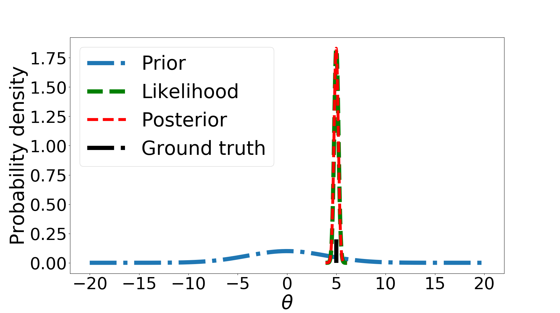
(a) Case (1): $\mathbf{\mathit{\theta}}_{\ast}=5$

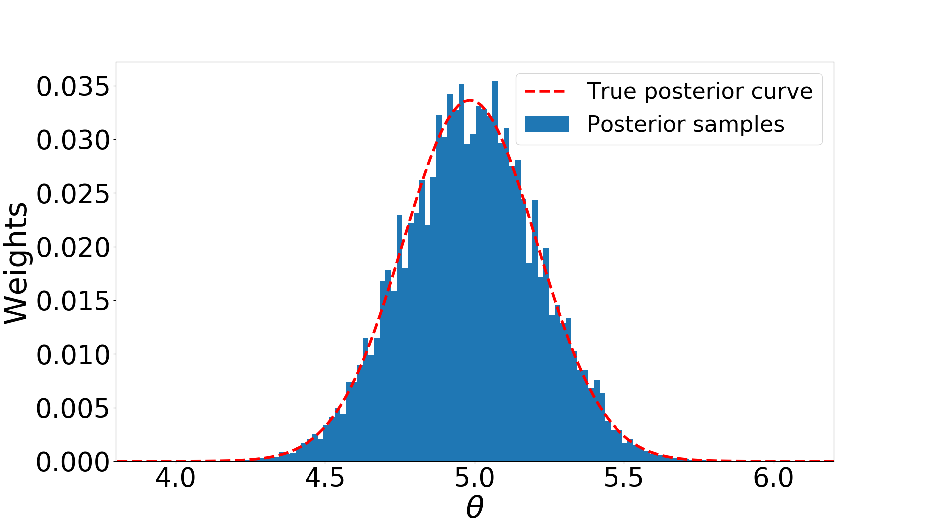
(b) Case (1) estimation

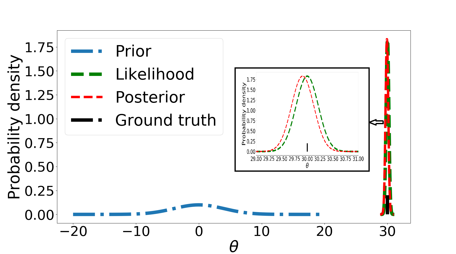
(c) Case (2): $\mathbf{\mathit{\theta}}_{\ast}=30$

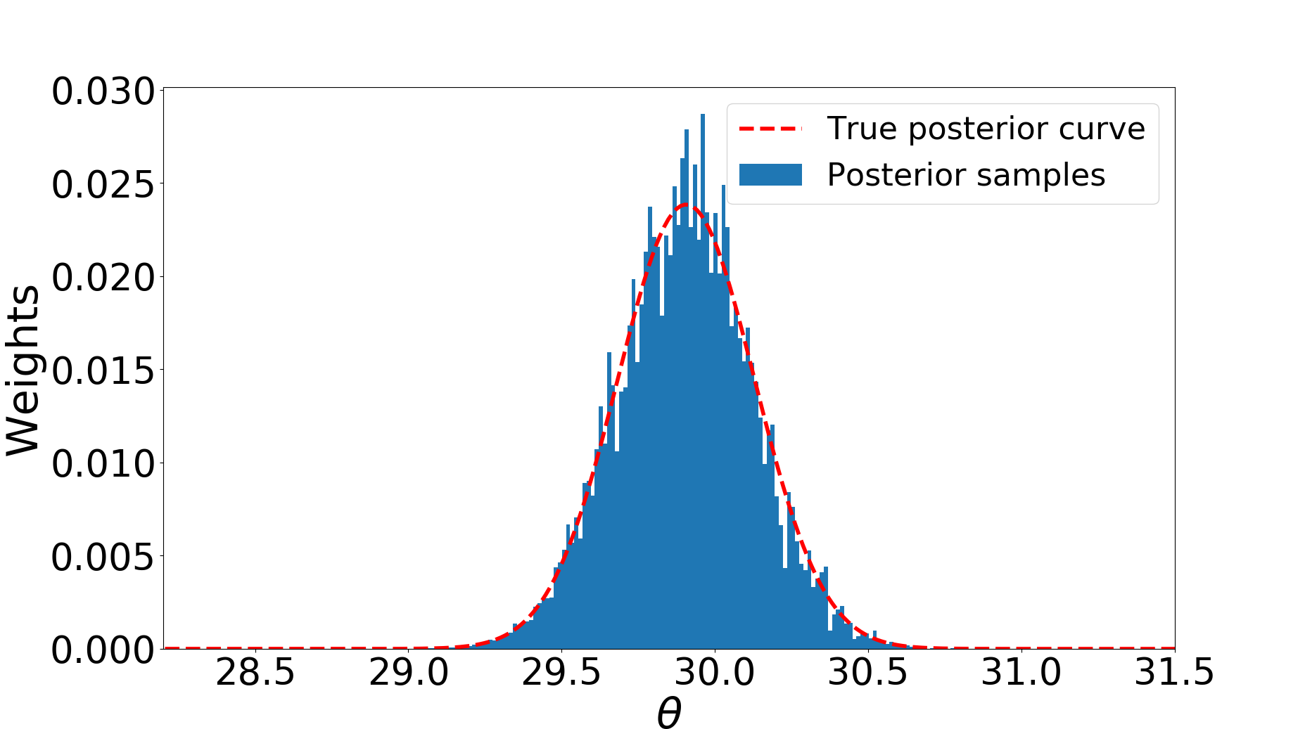
(d) Case (2) estimation

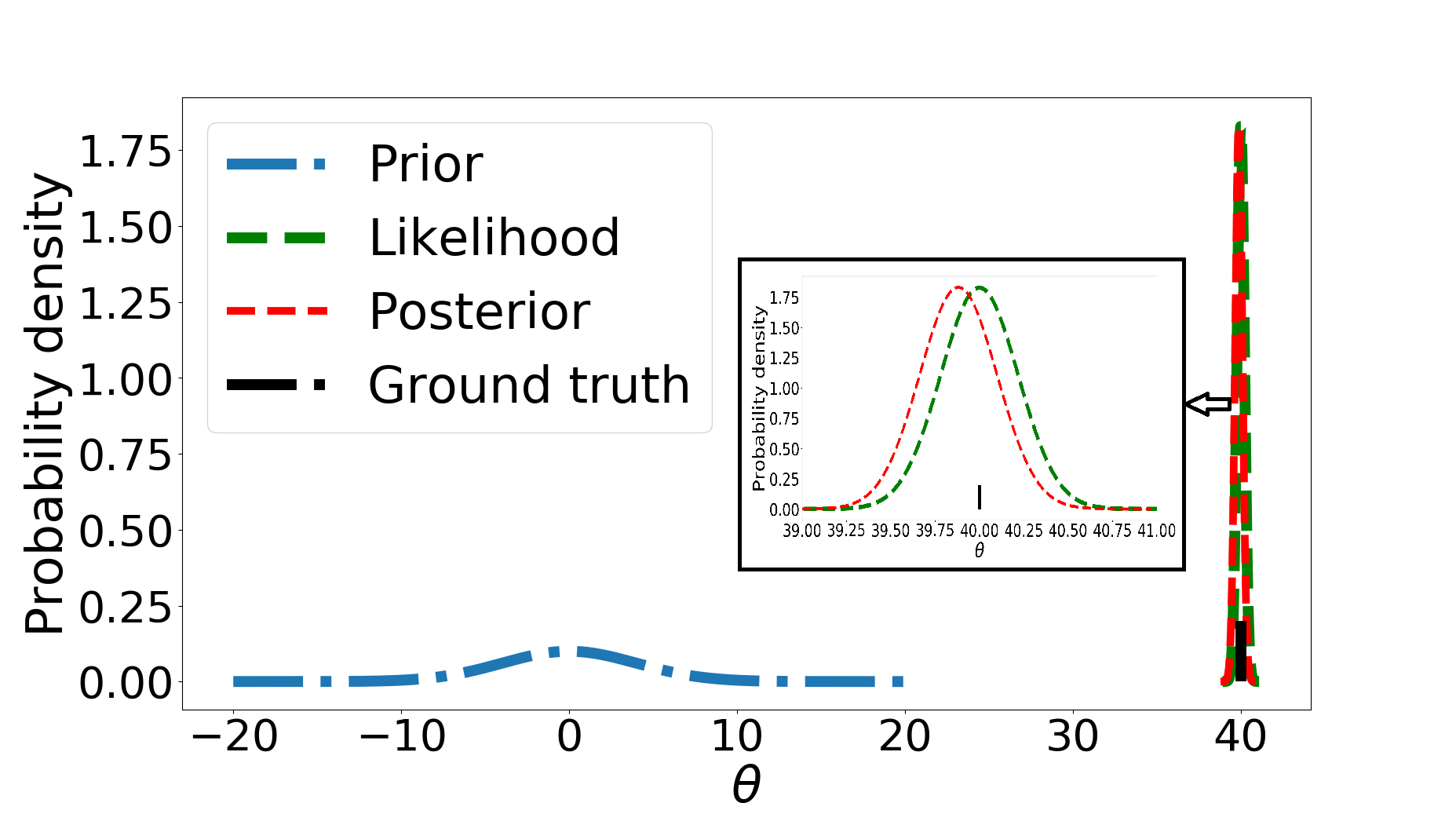
(e) Case (3): $\mathbf{\mathit{\theta}}_{\ast}=40$

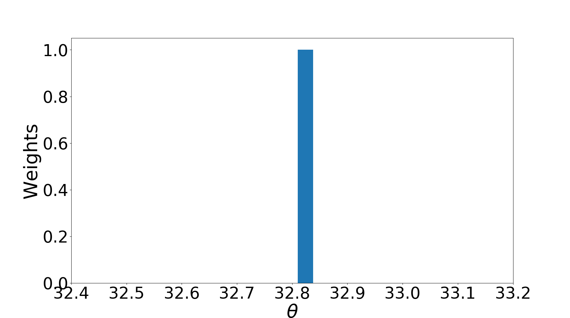
(f) Case (3) estimation

Figure 1: A univariate toy example illustrating the unrepresentative prior problem. Sub-figures (a), (c) and (e) show, respectively, the cases (1), (2) and (3) discussed in the text; sub-figures (c) and (e) contain zoomed-in plots. The truth $\mathbf{\mathit{\theta}}_{\ast}$ in each case is $\mathbf{\mathit{\theta}}_{\ast}=5$, $\mathbf{\mathit{\theta}}_{\ast}=30$ and $\mathbf{\mathit{\theta}}_{\ast}=40$, respectively (dashed black lines). The prior (dashed blue curves) is a Gaussian distribution with $\mu_{\mathit{\pi}}=0$ and $\sigma_{\mathit{\pi}}=4$. The likelihood (dashed green curves) is a Gaussian (5) with $\mu_{\mathit{\xi}}=1$. According to Bayes theorem (2), the posterior (dashed red curves) is also a Gaussian calculated from the product of prior and likelihood. Sub-figures (b), (d) and (f) show, for each case, the histogram (blue bins) of posterior samples from MultiNest, and the true posterior distribution (solid red curves).

To illustrate the problem of an unrepresentative prior, we consider three cases in which the true value $\mathbf{\mathit{\theta}}_{\ast}$ of the unknown parameter is given, respectively, by: (1) $\mathbf{\mathit{\theta}}_{\ast}=5$, (2) $\mathbf{\mathit{\theta}}_{\ast}=30$ and (3) $\mathbf{\mathit{\theta}}_{\ast}=40$. Thus, case (1) corresponds to a straightforward situation in which the true value $\mathbf{\mathit{\theta}}_{\ast}$ lies comfortably within the prior, whereas cases (2) and (3) represent the more unusual eventuality in which the true value lies well into the wings of the prior distribution. In our simple synthetic example, one expects cases (2) and (3) to occur only extremely rarely. In real-world applications, however, the prior distribution is typically constructed on a case-by-case basis by analysts, and may not necessarily support a standard frequentist’s interpretation of the probability of ‘extreme’ events. In fact, such situations are regularly encountered in real-world applications, when a large number of datasets are analysed. In each of the three cases considered, we set the variance of the simulated measurement noise to be $\sigma_{\mathit{\xi}}=1$ and the number of measurements is $N=20$. Note that the width of the likelihood in (5) is proportional to $1/\sqrt{N}$, so the unrepresentative prior problem becomes more acute as $N$ increases.

Figures 1 (a), (c) and (e) show the prior, likelihood and posterior distributions for the cases (1), (2) and (3), respectively. One sees that as the true value $\mathbf{\mathit{\theta}}_{\ast}$ increases and lies further into the wings of the prior, the posterior lies progressively further to the left of the likelihood, as expected. As a result, in cases (2) and (3), the peak of the posterior (red dashed curve) is displaced to the left of the true value (black dashed line). This can be clearly observed in the zoomed-in plots within sub-figures (c) and (e). Figures 1 (b), (d) and (f) show histograms (blue bins) of the posterior samples obtained using MultiNest for cases (1), (2) and (3), respectively, together with the corresponding true analytical posterior distributions (red solid curves). In each case, the MultiNest sampling parameters were set to $N_{\rm live}=2000$, ${\rm efr}=0.8$ and ${\rm tol}=0.5$ (see Feroz et al 2009 for details), and the algorithm was run to convergence. A natural estimator $\hat{\mathbf{\mathit{\theta}}}$ and uncertainty $\Delta\mathbf{\mathit{\theta}}$, respectively, for the value of the unknown parameter are provided by the mean and standard deviation of the posterior samples in each case, and are given in Table 1.

In case (1), one sees that the samples obtained are indeed consistent with being drawn from the true posterior, as expected. The mean $\hat{\mathbf{\mathit{\theta}}}$ and standard deviation $\Delta\mathbf{\mathit{\theta}}$ of the samples listed in Table 1 agree well with the mean $\mu_{\mathcal{P}}$ and standard deviation $\sigma_{\mathcal{P}}$ of the true posterior distribution. In this case, MultiNest converged relatively quickly, requiring a total of $13529$ likelihood evaluations. On repeating the entire analysis a total of 10 times, one obtains statistically consistent results in each case.

In case (2), one sees that the samples obtained are again consistent with being drawn from the true posterior. Indeed, from Table 1, one may verify that the mean and standard deviation of the samples agree well with those of the true posterior distribution. In this case, however, the convergence of MultiNest is much slower, requiring about 6 times the number of likelihood evaluations needed in case (1). This is a result of the true value lying far out in the wings of the prior distribution. Recall that NS begins by drawing $N_{\rm live}$ samples from the prior and at each subsequent iteration replaces the sample having the lowest likelihood with a sample again drawn from the prior but constrained to have a higher likelihood. Thus, as the iterations progress, the collection of $N_{\rm live}$ ‘live points’ gradually migrates from the prior to the peak of the likelihood. When the likelihood is concentrated very far out in the wings of the prior, this process can become very slow, even if one is able to draw each new sample from the constrained prior using standard methods (sometimes termed perfect nested sampling). In practice, this is usually not possible, so algorithms such as MultiNest and PolyChord use other methods that may require several likelihood evaluations before a new sample is accepted. Depending on the method used, an unrepresentative prior can also result in a significant drop in sampling efficiency, thereby increasing the required number of likelihood evaluations still further. On repeating the entire analysis a total of 10 times, once again obtains statistically consistent results in each case.

In case (3), one sees that the samples obtained are clearly inconsistent with being drawn from the true posterior. Indeed, the samples are concentrated at just a single value of $\mathbf{\mathit{\theta}}$. This behaviour may be understood by again considering the operation of NS. The algorithm begins by drawing $N_{\rm live}=2000$ samples from the prior, which is a Gaussian with mean $\mu_{\mathit{\pi}}=0$ and standard deviation $\sigma_{\mathit{\pi}}=4$. Thus, one would expect approximately only one such sample to lie outside the range $[-14,14]$. Moreover, since the likelihood is a Gaussian centred near the true value $\mathbf{\mathit{\theta}}_{\ast}=40$ with standard deviation $\sim 0.25$, the live points will typically all lie in a region over which the likelihood is very small and flat (although, in this particular example, the values of the log-likelihood for the live points – which is the quantity used in the numerical calculations – are still distinguishable to machine precision).

When the point with the lowest likelihood value is discarded, it must be replaced at the next NS iteration by another drawn from the prior, but with a larger likelihood. How this replacement sample is obtained depends on the particular NS implementation being used. As discussed in Section 2, MultiNest draws candidate replacement samples at each iteration using rejection sampling from within a multi-ellipsoid bound approximation to the iso-likelihood surface defined by the discarded point, which in just one dimension reduces simply to a range in $\mathbf{\mathit{\theta}}$. Since this bound is constructed from the samples present at that iteration, it will typically not extend far beyond the locations of the live points having the extreme values of the parameter $\mathbf{\mathit{\theta}}$. Thus, there is very limited opportunity to sample candidate replacement points from much larger values of $\mathbf{\mathit{\theta}}$, where the likelihood is significantly higher. Hence, as the NS iterations proceed, the migration of points from the prior towards the likelihood is extremely slow. Indeed, in this case, the migration is sufficiently slow that the algorithm terminates (in this case after $96512$ likelihood evaluations) before reaching the main body of the likelihood and produces a set of posterior-weighted samples from the discarded points (see Feroz et al 2009 for details). Since this weighting is proportional to the likelihood, in this extreme case the recovered posterior is merely a ‘spike’ corresponding to the sample with the largest likelihood, as observed in Figure 1 (f). In short, the algorithm has catastrophically failed. On repeating the entire analysis a total of 10 times, one finds similar pathological behaviour in each case.

One may, of course, seek to improve the performance of NS in such cases in a number of ways. Firstly, one may adjust the convergence criterion (tol in MultiNest) so that many more NS iterations are performed, although there is no guarantee in any given problem that this will be sufficient to prevent premature convergence. Perhaps more useful is to ensure that there is a greater opportunity at each NS iteration of drawing candidate replacement points from larger values of $\mathbf{\mathit{\theta}}$, where the likelihood is larger. This may be achieved in a variety of ways. In MultiNest, for example, one may reduce the $\tt{efr}$ parameter so that the volume of the ellipsoidal bound (or the $\mathbf{\mathit{\theta}}$-range in this one-dimensional problem) becomes larger. Alternatively, as in other NS implementations, one may draw candidate replacement points using either MCMC sampling (Feroz and Hobson, 2008) or slice-sampling (Handley et al, 2015) and increase the number of steps taken before a candidate point is chosen.

All the of above approaches may mitigate the problem to some degree in particular cases (as we have verified in further numerical tests), but only at the cost of a simultaneous dramatic drop in sampling efficiency caused precisely by the changes made in obtaining candidate replacement points. Moreover, in more extreme cases these measures fail completely. In particular, if the prior and the likelihood are extremely widely separated, the differences in the values of the log-likelihood of the live samples may fall below the machine accuracy used to perform the calculations. Thus, the original set of prior-distributed samples are likely to have log-likelihood values that are indistinguishable to machine precision. Thus, the ‘lowest likelihood’ sample to be discarded will be chosen effectively at random. Moreover, in seeking a replacement sample that is drawn from the prior but having a larger likelihood, the algorithm is very unlikely to obtain a sample for which the likelihood value is genuinely larger to machine precision. Even if such a sample is obtained, then the above problems will re-occur in the next iteration when seeking to replace the next discarded sample, and so on. In this scenario, the sampling efficiency again drops dramatically, but more importantly the algorithm essentially becomes stuck and will catastrophically fail because of accumulated numerical inaccuracies.

Table 1: MultiNest performance in the toy example illustrated in Figure 1.

	Case (1)	Case (2)	Case (3)
True value $\theta_{\ast}$	5	30	40
True posterior $\mu_{\cal{P}}$	4.984	29.907	39.875
True posterior $\sigma_{\cal{P}}$	0.223	0.223	0.223
Likelihood calls	13529	78877	96512
Estimated value $\hat{\mathbf{\mathit{\theta}}}$	4.981	29.902	32.838
Uncertainty $\Delta\mathbf{\mathit{\theta}}$	0.223	0.223	$7.6\text{\times}{10}^{-6}$

3.2 Simple ‘solutions’

A number of potential simple ‘solutions’ to the unrepresentative prior problem are immediately apparent. For example, one might consider the following:

• modify the prior distribution across one’s analysis, either by increasing its standard deviation $\sigma_{\pi}$, or even by adopting a different functional form, so that it should comfortably encompass the likelihood for all datasets;

• perform the analysis using the original prior for all the datasets, identify the datasets for which it is unrepresentative by monitoring the sampling efficiency and examining the final set of posterior samples for pathologies, and then modify the prior as above for these datasets.

Unfortunately, neither of these approaches is appropriate or realistic. The former approach is inapplicable since the prior may be representative for the vast majority of the datasets under analysis, and one should use this information in deriving inferences. Also, the former solution sacrifices the overall speed and computational efficiency, as the augmented prior is applied to all cases but not only the problematic ones. Choosing a proper trade-off between the efficiency and the coverage of prior is difficult when a large number of experiments need to be examined.

The latter solution requires one to identify various outlier cases (as the outlier cases could be very different from one to another), and also perform re-runs of those identified. It becomes a non-trivial computational problem when a single algorithm run requires a considerable amount of run time, or when the results of the outlier cases are needed for the next step computation, i.e. the whole process waits for the outlier cases to proceed. This could be trivial for some applications and could be very difficult for others in which many different outlier cases exist.

4 Posterior repartitioning method

The posterior repartitioning (PR) method addresses the unrepresentative prior problem in the context of NS algorithms (Skilling, 2006) for exploring the parameter space, without sacrificing computational speed or changing the inference obtained.

4.1 General expressions

In general, the ‘repartition’ of the product $\mathcal{L}(\mathbf{\mathit{\theta}})\pi(\mathbf{\mathit{\theta}})$ can be expressed as:

$$\mathcal{L}(\mathbf{\mathit{\theta}})\mathit{\pi}(\mathbf{\mathit{\theta}})=\tilde{\mathcal{L}}(\mathbf{\mathit{\theta}})\tilde{\mathit{\pi}}(\mathbf{\mathit{\theta}}),$$ (6)

where $\tilde{\mathcal{L}}(\mathbf{\mathit{\theta}})$ and $\tilde{\mathit{\pi}}(\mathbf{\mathit{\theta}})$ are the new effectivelikelihood and prior, respectively. As a result, the (unnormalised) posterior remains unchanged. The modified prior $\tilde{\mathit{\pi}}(\mathbf{\mathit{\theta}})$ can be any tractable distribution, which we assume to be appropriately normalised to unit volume. The possibility of repartitioning the posterior in NS was first mentioned in Feroz et al (2009), but equation (6) can also be viewed as the vanilla case (when the importance weight function equals to $1$) of nested importance sampling proposed in Chopin and Robert (2010).

One general advantage of NS is that the evidence (or marginal likelihood), which is intractable in most cases, can be accurately approximated. This is achieved by first defining $\mathit{V}(\mathit{l})$ as the prior volume within the iso-likelihood contour $\mathcal{L}(\mathbf{\mathit{\theta}})=\mathit{l}$, namely

$$\mathit{V}(\mathit{l})=\int_{\mathcal{L}(\mathbf{\mathit{\theta}})>\mathit{l}}\mathit{\pi}(\mathbf{\mathit{\theta}})d\mathbf{\mathit{\theta}},$$ (7)

where $\mathit{l}$ is a real number that gradually rises from zero to the maximum of $\mathcal{L}(\mathbf{\mathit{\theta}})$ as the NS iterations progress, so that $\mathit{V}(\mathit{l})$ monotonically decreases from unity to zero. After PR, $\mathit{\pi}(\mathbf{\mathit{\theta}})$ is replaced by $\tilde{\mathit{\pi}}(\mathbf{\mathit{\theta}})$, and the evidence can be calculated as

$$\mathcal{Z}=\int\mathcal{L}(\mathbf{\mathit{\theta}})\mathit{\pi}(\mathbf{\mathit{\theta}})d\mathbf{\mathit{\theta}}=\int\tilde{\mathcal{L}}(\mathbf{\mathit{\theta}})\tilde{\mathit{\pi}}(\mathbf{\mathit{\theta}})d\mathbf{\mathit{\theta}}=\int_{0}^{1}\mathcal{L}(\mathit{V})d\mathit{V}.$$ (8)

It is worth noting, however, that in the case where $\tilde{\mathit{\pi}}(\mathbf{\mathit{\theta}})$ is not properly normalised, the ‘modified evidence’ $\mathcal{Z}^{\prime}$ obtained after PR is simply related to the original evidence by

$$\mathcal{Z}=\mathcal{Z}^{\prime}\int\tilde{\mathit{\pi}}(\mathbf{\mathit{\theta}})d\mathbf{\mathit{\theta}}.$$ (9)

Provided one can evaluate the volume of the modified prior $\tilde{\mathit{\pi}}(\mathbf{\mathit{\theta}})$, one may therefore straightforwardly recover the original evidence, if required. For many simple choices of $\tilde{\mathit{\pi}}(\mathbf{\mathit{\theta}})$, this is possible analytically, but may require numerical integration in general. It should be noted, however, that the normalistion of the modified prior is irrelevant for obtaining posterior samples. We now discuss some particular special choices for $\tilde{\mathit{\pi}}(\mathbf{\mathit{\theta}})$.

4.2 Power posterior repartitioning

Rather than introducing a completely new prior distribution into the problem, a sensible choice is often simply to take $\tilde{\mathit{\pi}}(\mathbf{\mathit{\theta}})$ to be the original prior $\mathit{\pi}(\mathbf{\mathit{\theta}})$ raised to some power, and then renormalised to unit volume, such that

$$\tilde{\mathit{\pi}}(\mathbf{\mathit{\theta}}) =\frac{\mathit{\pi}(\mathbf{\mathit{\theta}})^{\mathit{\beta}}}{\mathcal{Z}_{\pi}(\beta)},$$ (10)

$$\tilde{\mathcal{L}}(\mathbf{\mathit{\theta}}) =\mathcal{L}(\mathbf{\mathit{\theta}})\mathit{\pi}(\mathbf{\mathit{\theta}})^{(1-\mathit{\beta})}\mathcal{Z}_{\pi}(\beta),$$ (11)

where $\mathit{\beta}\in[0,1]$ and $\mathcal{Z}_{\pi}(\beta)\equiv\int\mathit{\pi}(\mathbf{\mathit{\theta}})^{\mathit{\beta}}d\mathbf{\mathit{\theta}}$. By altering the value of $\mathit{\beta}$, the modified prior can be chosen from a range between the original prior ($\mathit{\beta}=1$) and the uniform distribution ($\mathit{\beta}=0$). As long as the equality in equation (6) holds, the PR method can be applied separately for multiple unknown parameters with different forms of prior distributions.

Figure 2 illustrates how the prior changes for different values of $\mathit{\beta}$ in a one-dimensional problem. As the parameter $\mathit{\beta}$ decreases from $1$ to $0$, the prior distribution evolves from a Gaussian centred on zero with standard deviation $\sigma_{\pi}=4$ to a uniform distribution, where the normalisation depends on the assumed support $[-50,50]$ of the unknown parameter $\mathbf{\mathit{\theta}}$. Indeed, the uniform modified prior $\tilde{\mathit{\pi}}(\mathbf{\mathit{\theta}})\sim\mathcal{U}(a,b)$ is a special case, but often a useful choice. One advantage of this choice is that the range $[a,b]$ can be easily set such that it accommodates the range of $\mathbf{\mathit{\theta}}$ values required to overcome the unrepresentative prior problem, and the modified prior is trivially normalised. It can cause the sampling to be inefficient, however, since it essentially maximally broadens the search space (within the desired range).

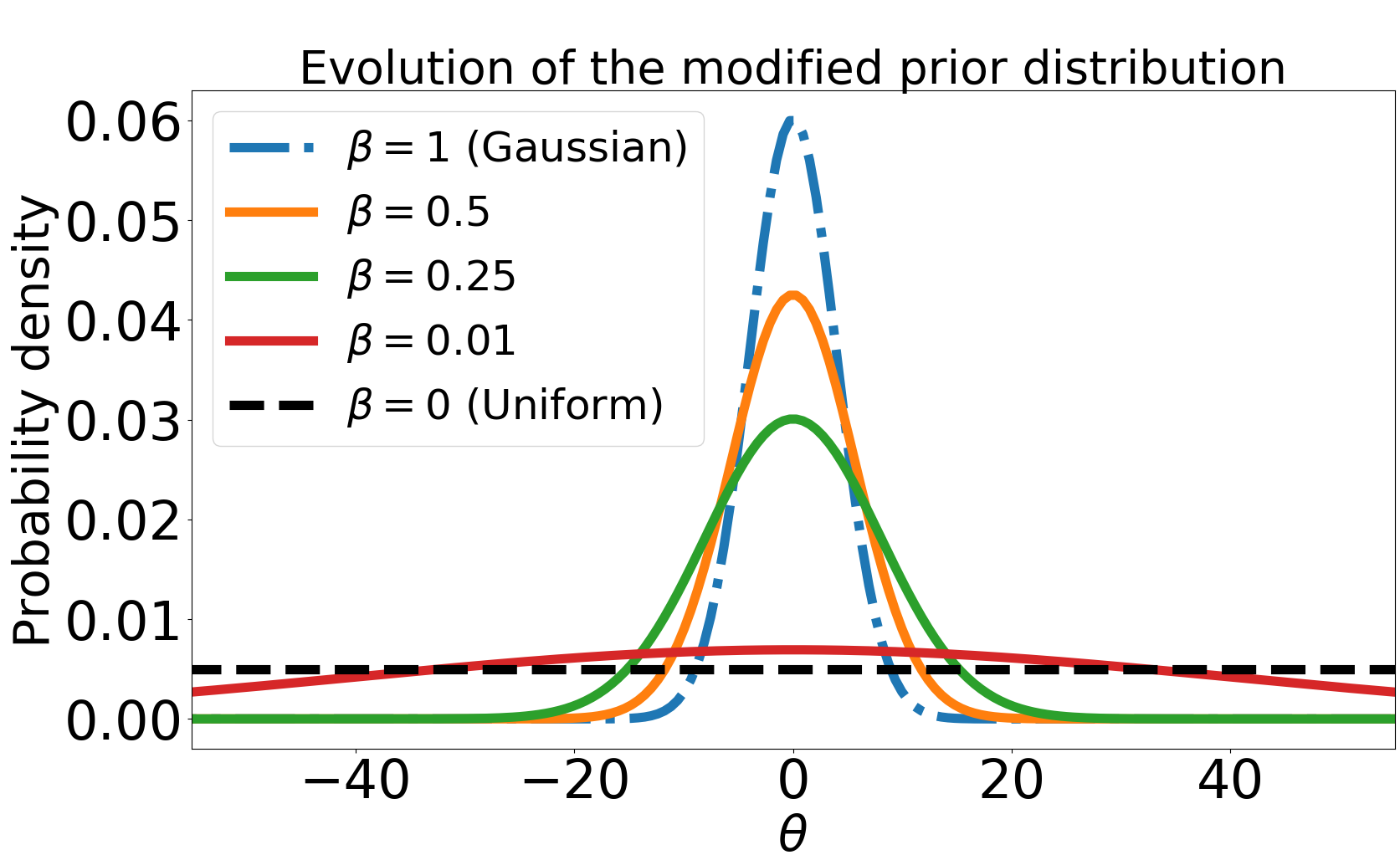
Figure 2: One dimensional prior evolution for $\mathit{\beta}\in[0,1]$. The original prior is a Gaussian distribution with $\sigma_{\pi}=4$ (truncated in the range $[-50,50]$) when $\mathit{\beta}=1$ (dashed blue curve), and is an uniform distribution when $\mathit{\beta}=0$ (dashed black curve). The remaining three curves correspond to $\mathit{\beta}=0.5$ (green curve), $0.25$ (red curve), $0.01$ (light blue curve), respectively.

The above approach is easily extended to multivariate problems with parameter vector $\bm{\theta}=(\mathbf{\mathit{\theta}}_{1},\mathbf{\mathit{\theta}}_{2},\cdots,\mathbf{\mathit{\theta}}_{N})^{\rm T}$. It is worth noting in particular the case where the original prior is a multivariate Gaussian, such that $\mathit{\pi}(\bm{\theta})=\mathcal{N}(\bm{\mathit{\mu}},\bm{\Sigma})$, where $\bm{\mathit{\mu}}$ is the vector of means for each variable and $\bm{\Sigma}$ is the covariance matrix. The power modified prior $\tilde{\mathit{\pi}}(\bm{\theta})$ is then given simply by $\mathcal{N}(\bm{\mathit{\mu}},\mathit{\beta}^{-1}\bm{\Sigma})$ over the assumed supported region $\mathcal{R}$ of the parameter space, and

$$\mathcal{Z}_{\pi}(\beta)=(2\mathit{\pi})^{\frac{\mathit{N}}{2}(1-\mathit{\beta})}|\bm{\Sigma}|^{\frac{(1-\mathit{\beta})}{2}}\mathit{\beta}^{-\frac{\mathit{N}}{2}}\int_{\mathcal{R}}\mathcal{N}(\bm{\mathit{\mu}},\mathit{\beta}^{-1}\bm{\Sigma})d\bm{\theta}.$$ (12)

There is unfortunately no robust universal guideline for choosing an appropriate value for $\mathit{\beta}$, since this depends on the dimensionality and complexity of the posterior and on the initial prior distribution assumed. Nonetheless, as demonstrated in the numerical examples presented in Section 5, there is a straightforward approach for employing the PR method in more realistic problems, in which the true posterior is not known. Namely, starting from $\mathit{\beta}=1$ (which corresponds to the original prior), one can obtain inferences for progressively smaller values of $\mathit{\beta}$, according to some pre-defined or dynamic ‘annealing schedule’, until the results converge to a statistically consistent solution. The precise nature of the annealing schedule is unimportant, although either linearly or exponentially decreasing values of $\mathit{\beta}$ seem the most natural approaches.

4.3 More general posterior repartitioning

Raising the original prior to some power $\beta$ merely provides a convenient way of defining the modified prior, since it essentially just broadens the original prior by some specified amount. In general, however, $\tilde{\mathit{\pi}}(\mathbf{\mathit{\theta}})$ can be any tractable distribution. For example, there is no requirement for the modified prior to be centred at the same parameter value as the original prior. One could, therefore, choose a modified prior that broadens and/or shifts the original one, or a modified prior that has a different form from the original. Note that, in this generalised setting, the modified prior should at least be non-zero everywhere that the original prior is non-zero.

4.4 Diagnostics of the unrepresentative prior problem

This paper focuses primarily on how to mitigate the unrepresentative prior problem using PR. Another critical issue, however, is how one may determine when the prior is unrepresentative in the course the analysis of some (large number of) dataset(s). We comment briefly on this issue here.

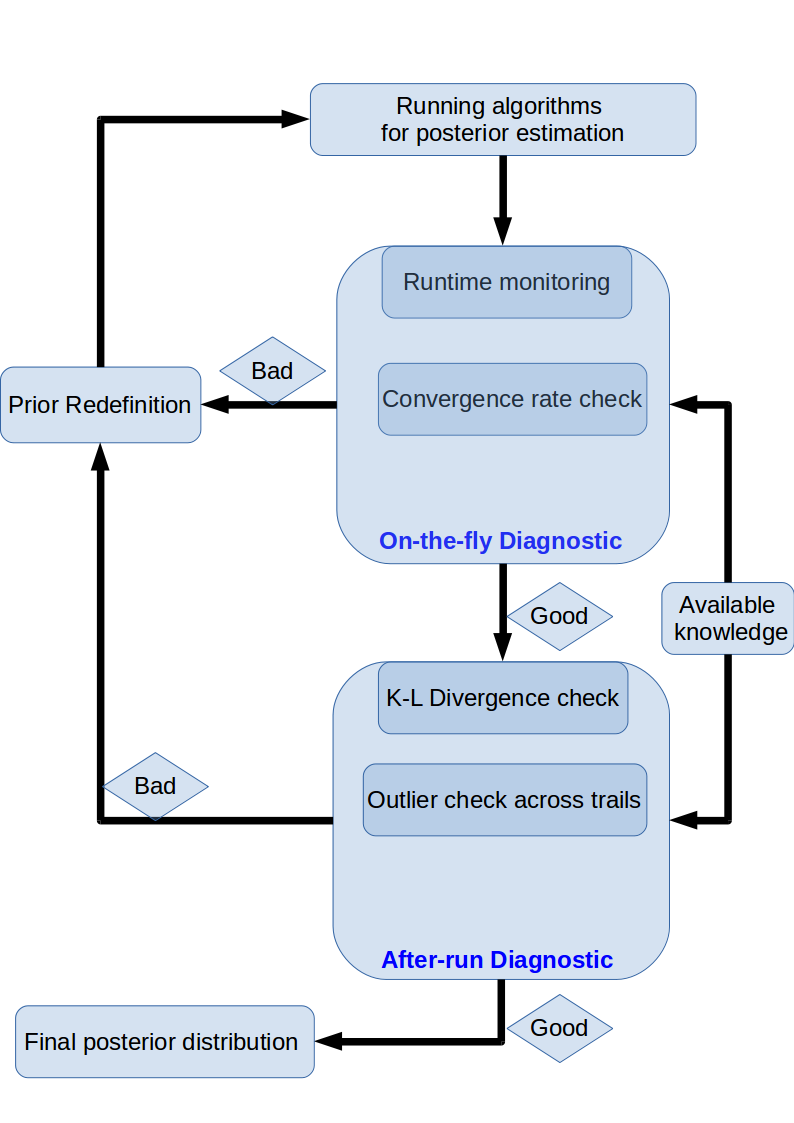
Figure 3: A flow chart of a designed diagnostic process. The two main steps of the diagnostic process are highlighted in dark blue. The process starts by running a sampling algorithm for Bayesian parameter estimation (the top small block), and proceeds with two hierarchical diagnostics steps to evaluate the trail of interest. ‘Available knowledge’ is defined as reliable experimental information and prior knowledge that one could obtain in advance.

Diagnosing the unrepresentative prior problem beforehand is generally difficult. Thus, designing a practical engineering-oriented solution is helpful in addressing most such problems. The goal of this diagnostic is to identify abnormal cases amongst a number of datasets during the analysis procedure. We assume that at least a few ‘reliable’ (sometimes called ‘gold standard’) datasets, which do not suffer from the unrepresentative prior problem, have been analysed before the diagnostics. The reliability threshold of a dataset varies depending on different scenarios, but (ideally) a gold standard dataset should: (1) be recognised as such by field experts; (2) have all of its noise sources clearly identified and characterised; (3) yield parameter estimates that are consistent with true values either known a priori or determined by other means. These provide us with some rough but reliable information and prior knowledge, such as runtime, convergence rate, and the shape of posterior distribution. We denote this information as the available knowledge for the problem of interest.

One may then employ a diagnostic scheme of the type illustrated in Figure 3, which is composed of two parts: on-the-fly diagnostics and after-run diagnostics. On-the-fly diagnostics involve monitoring the runtime and convergence status during the analysis of each dataset. Specifically, runtime monitoring involves simply checking whether the runtime of an individual analysis is greatly different from those of the available knowledge. Similarly, convergence rate checks compare the speed of convergence between the current run and the available knowledge. If both results are consistent with those in the available knowledge, the diagnostic process proceeds to after-run diagnostics. Note that the quantitative consistency check can be defined in various ways. A simple method is to set a threshold for the difference between available knowledge and individual runs. For instance, the result from an individual run can be considered as a reliable one if the error between the individual run result and the mean of the available knowledge is within a certain threshold. Such criteria should be carefully discussed by field experts on a case-by-case basis.

After-run diagnostics compare the computed posterior with the available knowledge. One plausible after-run diagnostic is to evaluate some ‘distance’ measure between the assumed prior and the posterior distribution resulting from the analysis. An obvious choice is to employ the Kullback–Leibler (KL) divergence (see, e.g., Bishop 2006). The KL divergence quantifies the difference between two probability distributions by calculating their relative entropy. A larger KL divergence indicates a greater difference between the two distributions. The KL divergence is, however, an asymmetric measure and its value is not bounded. To overcome these drawbacks, one could also consider the Jensen–Shannon divergence (Endres and Schindelin, 2003), which is a symmetric variant of the KL divergence. The posterior may also be compared with the available knowledge in the outlier check step.

Finally, we note that a diagnostic analysis is valid when it is performed using the same algorithm specifications. For instance, $N_{\rm live}$, ${\rm efr}$, and ${\rm tol}$ settings should be the same in MultiNest when performing diagnostic analysis. In any case, once a reasonable diagnostic metric is constructed, the abnormal trials can be identified according to some predetermined criteria and examined, and the proposed PR scheme can be applied on a case-by-case basis. A simple illustration of this process is presented in the bivariate example case in the next section.

5 Numerical examples

We begin by illustrating the PR method in two numerical examples, one univariate and the other a bivariate Gaussian posterior. Our investigation is then extended to higher dimensional (from 3 to 15 dimensions) Gaussian posteriors, to explore its stability to the ‘curse of dimensionality’. Finally, we consider a bivariate non-Gaussian example. In particular, we compare the performance of the MultiNest sampler before and after applying PR.

(a) $\mathbf{\mathit{\theta}}_{\ast}=40$, theoretical distribution

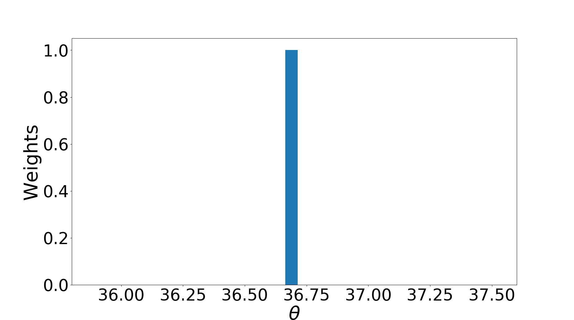
(b) $\mathit{\beta}=0.8$

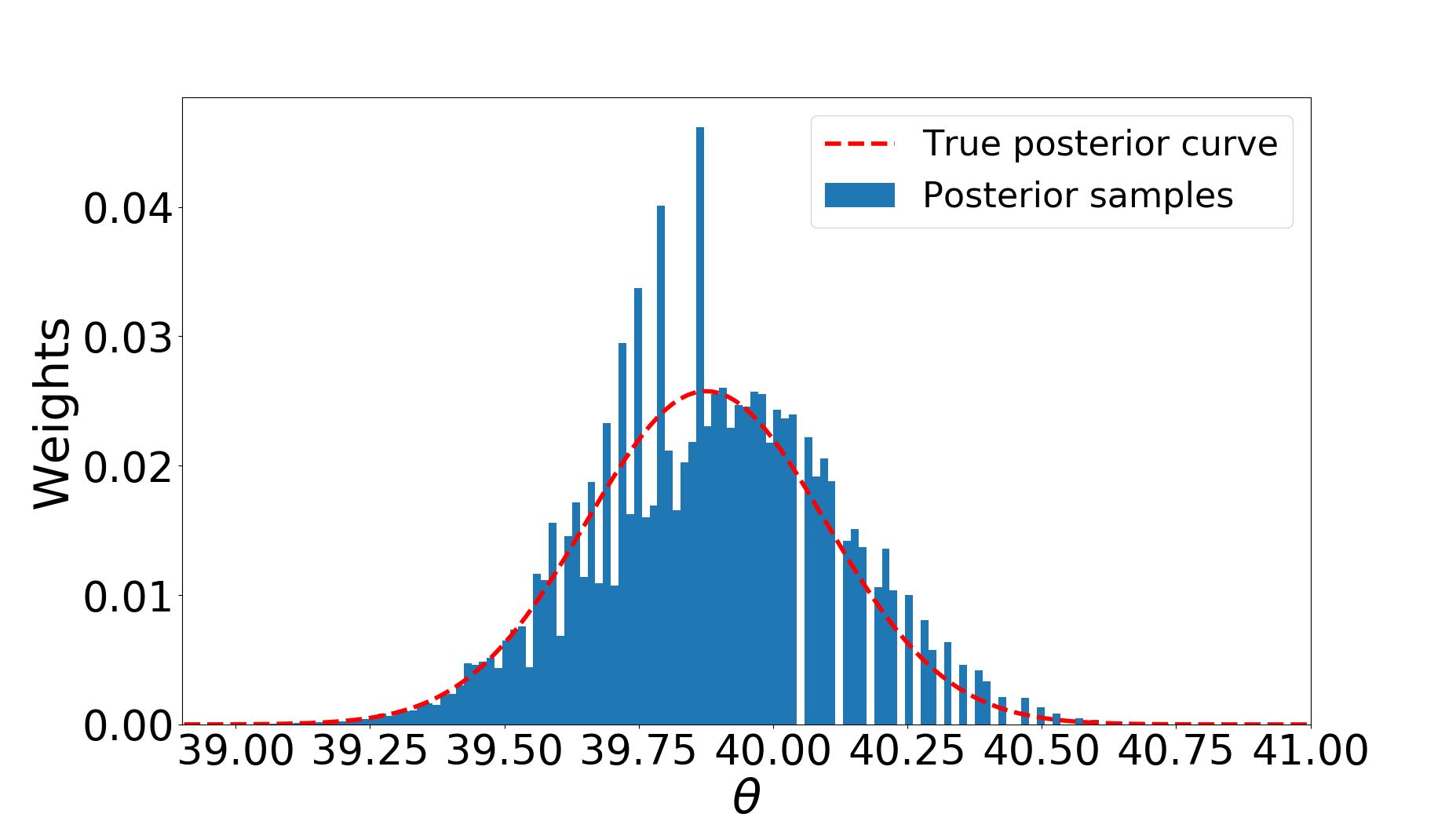
(c) $\mathit{\beta}=0.6$

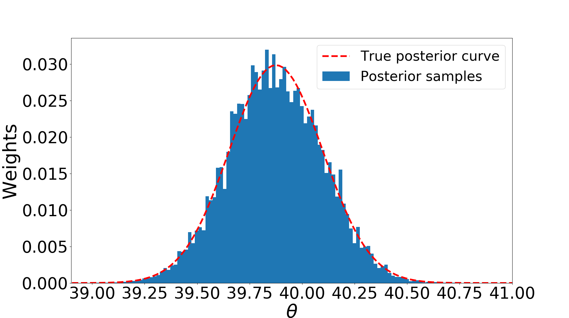
(d) $\mathit{\beta}=0.4$

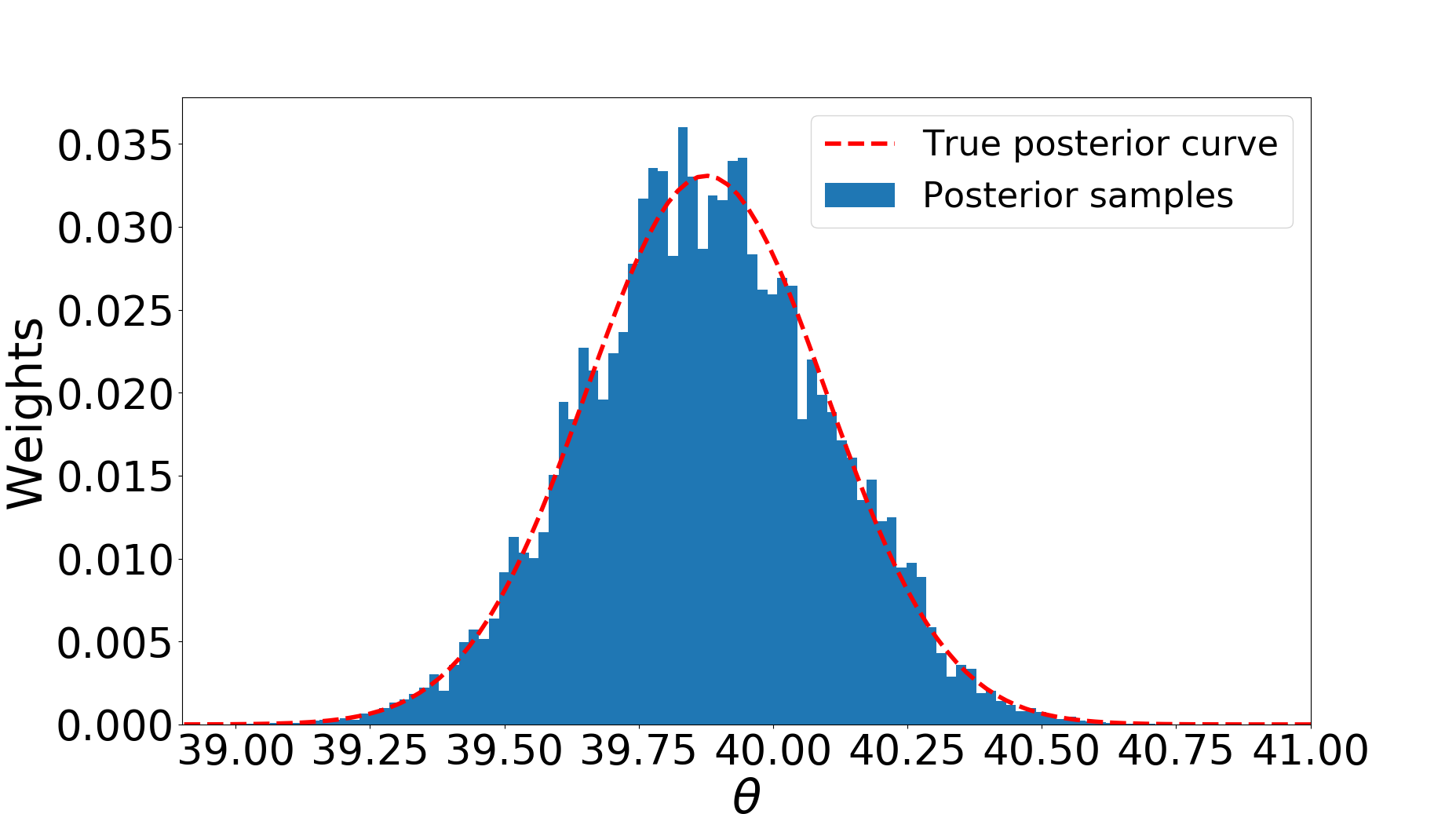
(e) $\mathit{\beta}=0.2$

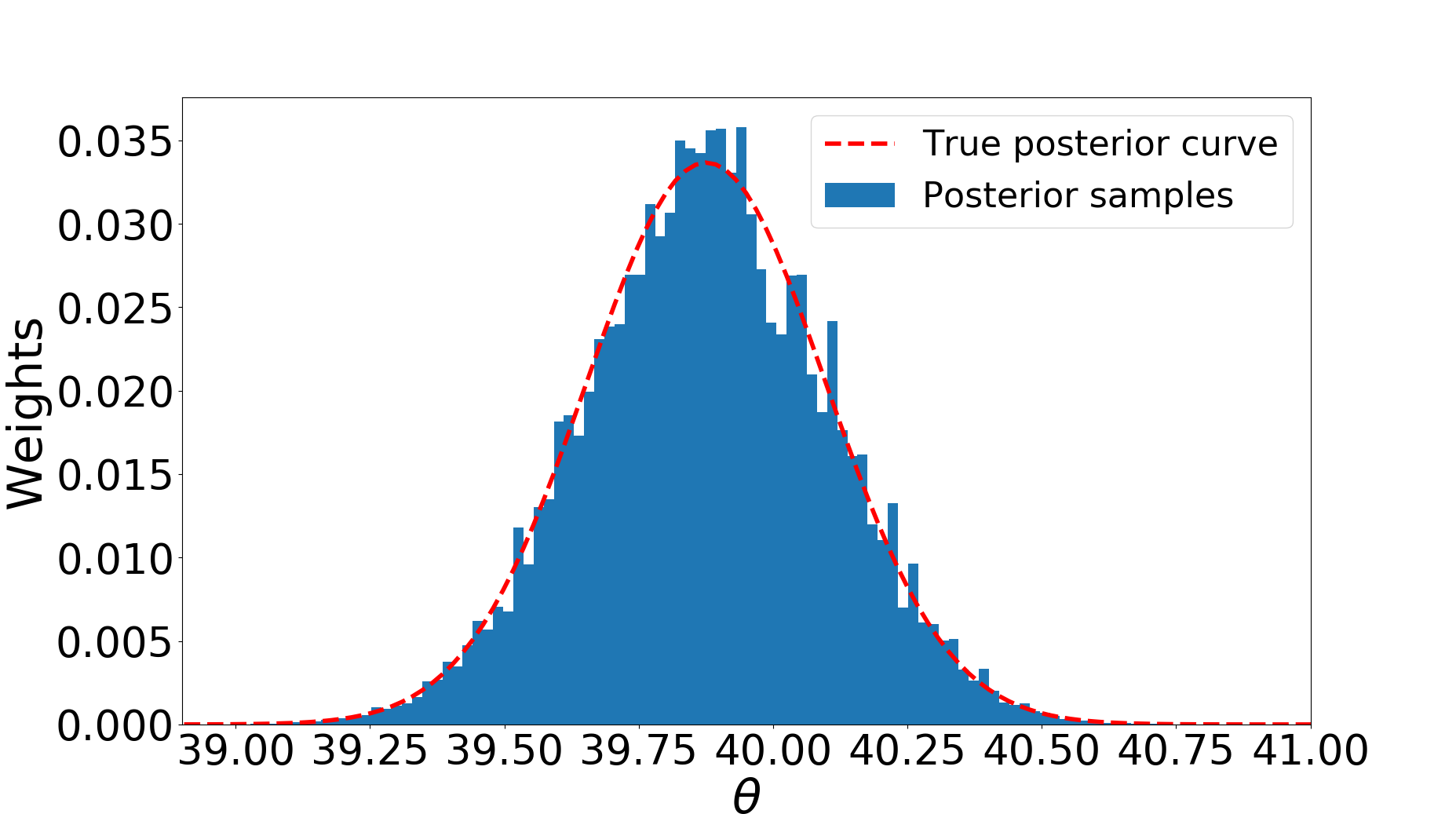
(f) $\mathit{\beta}=0$, uniform prior

Figure 4: MultiNest performance using the PR method with different $\mathit{\beta}$ values, applied to case (3) ($\mathbf{\mathit{\theta}}_{\ast}=40$) of the toy example discussed in Section 3.1; all other settings remain unaltered. The values $\mathit{\beta}=0.8,0.6,0.4,0.2,0$ are tested. Figure (a) shows the distribution of the prior (blue dashed curve), likelihood (green dashed curve), ground truth (black dashed line), and posterior (red dashed curve). The remaining five figures show the histograms (blue bins) of the posterior-weighted samples for the $\mathit{\beta}$ values tested and the true posterior distribution (red curve).

We use the open-source MultiNest package (Feroz et al, 2009) and set efficiency parameter ${\rm efr}=0.8$, convergence tolerance parameter ${\rm tol}=0.5$, multi-modal parameter ${\rm mmode}={\rm False}$, random seed control parameter ${\rm seed}=-1$, and the constant efficiency mode ${\rm ceff}={\rm False}$ for all the following examples. The number of live samples $N_{\rm live}$ varies in different cases. We keep the other MultiNest tuning options in their default values. See (Feroz et al, 2009) and its corresponding MultiNest Fortran package for details of these default settings.

In some of the multi-dimensional cases, we also compare the MultiNest performance with MCMC. Specifically, a standard Metropolis–Hastings sampler is implemented and applied to the same numerical examples. Other MCMC samplers such as No-U-Turn Sampler (NUTS), and slice samplers give similar performance in the numerical examples. One popular Python implementation of these samplers can be found in PyMC3 (Salvatier et al, 2016) package. In some cases, we also compare the performance of importance sampling (Neal, 2001; Tokdar and Kass, 2010; Martino et al, 2018), using a standard IS implementation from Python package ‘pypmc’ (Jahn et al, 2018).

5.1 Toy univariate example revisited

Here we re-use case (3) of the toy example discussed in Section 3.1, for which MultiNest was shown to fail without applying PR. In this case, the true value of the unknown parameter is $\mathbf{\mathit{\theta}}_{\ast}=40$ and the number of observations is set to $N=20$ (see Figure 4(a)).

We use power prior redefinition and consider the $\mathit{\beta}$ values $0,0.2,0.4,0.6,0.8$ and $1$; note that $\mathit{\beta}=1$ is equivalent to the original method implemented in the toy example, and $\mathit{\beta}=0$ corresponds to using a uniform distribution as the modified prior. The range of the uniform prior for $\mathit{\beta}=0$ is set as $\mathbf{\mathit{\theta}}\in[0,50]$ in this example.

Figure 4 shows the performance of MultiNest assisted by the PR method. Panels (b) to (f) show the MultiNest performance with decreasing $\mathit{\beta}$. One sees that as $\beta$ decreases, the posterior samples obtained approximate the true posterior with increasing accuracy, although in this extreme example one requires $\beta=0.4$ or lower to obtain consistent results.

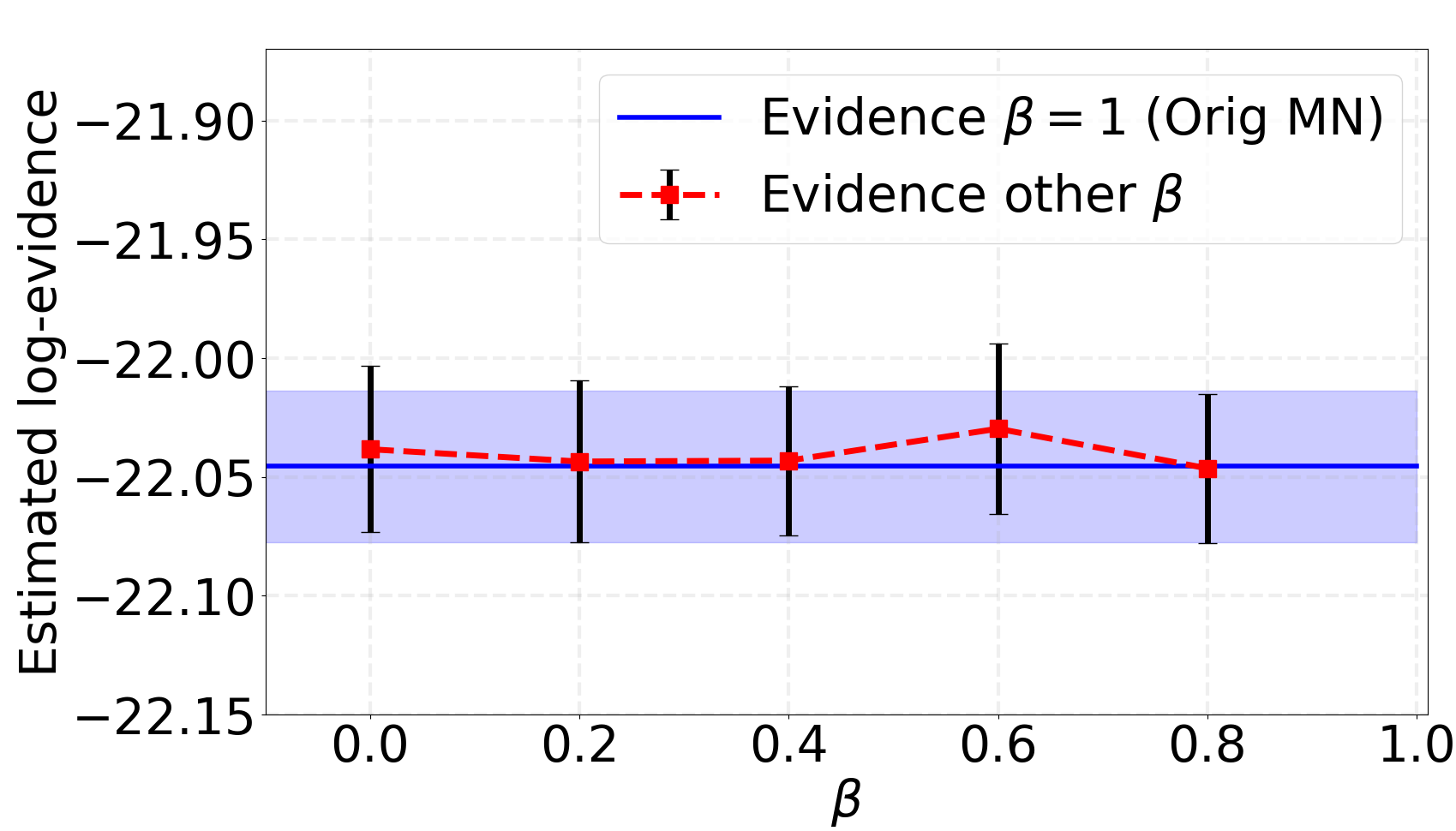
(a) case (1), $\bm{\theta}_{\ast}=5$

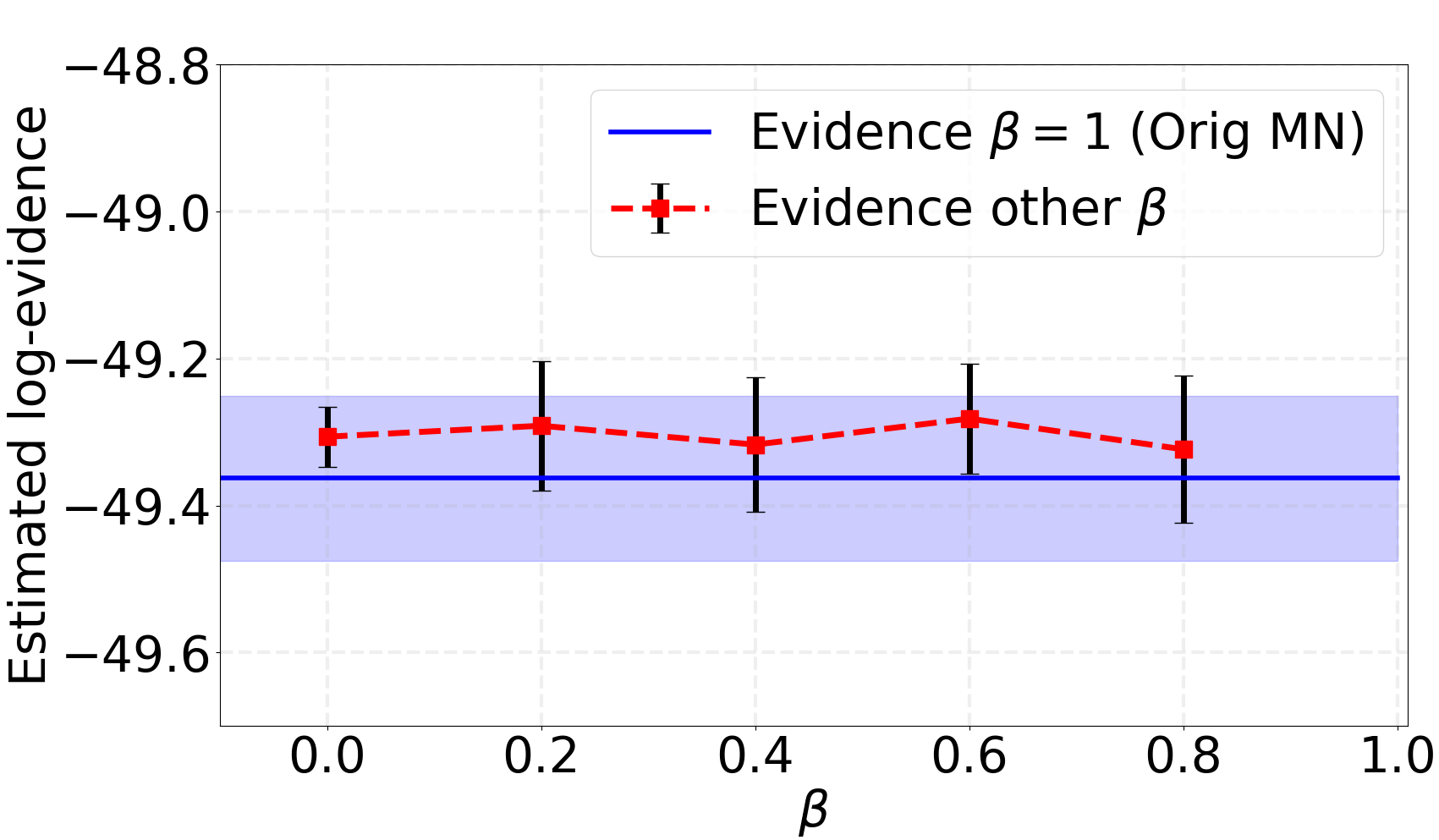
(b) case (2), $\bm{\theta}_{\ast}=30$

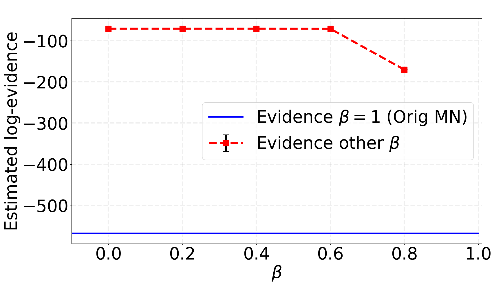
(c) case (3), $\bm{\theta}_{\ast}=40$

Figure 5: Evidence estimation versus $\mathit{\beta}$ for cases (1)–(3) of the univariate toy example. The blue solid line and the light blue shaded area indicate, respectively, the average and standard deviation of the log-evidence values produced by MultiNest without PR ($\mathit{\beta}=1$) from 20 realisations of the data. The red marker black cap errorbar shows the corresponding quantities produced using PR with $\mathit{\beta}=0,0.2,0.4,0.6,0.8,1$.

To evaluate the performance of the PR method further, MultiNest was run on 10 realisations for each value of $\mathit{\beta}$. The resulting histograms of MultiNest’s posterior samples were then fitted with a standard Gaussian distribution. For each value of $\mathit{\beta}$, the average of the means of the fitted Gaussian distributions and the root mean squared error (RMSE) between these estimates and the true value are presented in Table 2, along with the average number of likelihood calls for MultiNest to converge; since the time spent for each likelihood calculation is similar, this quantity is proportional to the runtime. The RMSE clearly decreases as $\mathit{\beta}$ decreases from unity to zero, which demonstrates that a wider prior allows MultiNest to obtain more accurate results, even in this extreme example of an unrepresentative prior. Also, one sees that the averaged number of likelihood evaluations also decreases significantly with $\mathit{\beta}$, so that the computational efficiency is also increased as the effective prior widens.

Table 2: A numerical comparison of the results in the univariate toy example of the PR method for different values of $\mathit{\beta}$ (where $\mathit{\beta}=1$ corresponds to the standard method). The quantity $\bar{\mu}$ denotes the averaged mean value of the fitted Gaussian distribution to the posterior histogram over 10 realisations. RMSE denotes the root mean squared error between the ground truth value and $\bar{\mu}$. ${\rm N_{like}}$ is the averaged number of likelihood evaluations, and $\mathcal{Z}$ denotes the averaged estimated log-evidence and its uncertainty given by MultiNest.

$\mathit{\beta}$	$\bar{\mu}$	RMSE	${\rm N_{like}}$	$\mathcal{Z}$
1	$32.838$	$7.037$	$96378$	$-567.5679\mathbin{\mathchoice{\ooalign{\raisebox{0.3pt}{$\displaystyle+$}\cr\smash{\raisebox{-0.4pt}{$\displaystyle-$}}\cr}}{\ooalign{\raisebox{0.3pt}{$\textstyle+$}\cr\smash{\raisebox{-0.4pt}{$\textstyle-$}}\cr}}{\ooalign{\raisebox{0.3pt}{$\scriptstyle+$}\cr\smash{\raisebox{-0.4pt}{$\scriptstyle-$}}\cr}}{\ooalign{\raisebox{0.3pt}{$\scriptscriptstyle+$}\cr\smash{\raisebox{-0.4pt}{$\scriptscriptstyle-$}}\cr}}}0.1346$
0.8	$36.714$	$3.161$	$93492$	$-170.3971\mathbin{\mathchoice{\ooalign{\raisebox{0.3pt}{$\displaystyle+$}\cr\smash{\raisebox{-0.4pt}{$\displaystyle-$}}\cr}}{\ooalign{\raisebox{0.3pt}{$\textstyle+$}\cr\smash{\raisebox{-0.4pt}{$\textstyle-$}}\cr}}{\ooalign{\raisebox{0.3pt}{$\scriptstyle+$}\cr\smash{\raisebox{-0.4pt}{$\scriptstyle-$}}\cr}}{\ooalign{\raisebox{0.3pt}{$\scriptscriptstyle+$}\cr\smash{\raisebox{-0.4pt}{$\scriptscriptstyle-$}}\cr}}}0.1347$
0.6	$39.870$	$0.005$	$83619$	$-71.1709\mathbin{\mathchoice{\ooalign{\raisebox{0.3pt}{$\displaystyle+$}\cr\smash{\raisebox{-0.4pt}{$\displaystyle-$}}\cr}}{\ooalign{\raisebox{0.3pt}{$\textstyle+$}\cr\smash{\raisebox{-0.4pt}{$\textstyle-$}}\cr}}{\ooalign{\raisebox{0.3pt}{$\scriptstyle+$}\cr\smash{\raisebox{-0.4pt}{$\scriptstyle-$}}\cr}}{\ooalign{\raisebox{0.3pt}{$\scriptscriptstyle+$}\cr\smash{\raisebox{-0.4pt}{$\scriptscriptstyle-$}}\cr}}}0.1276$
0.4	$39.872$	$0.003$	$61796$	$-70.9523\mathbin{\mathchoice{\ooalign{\raisebox{0.3pt}{$\displaystyle+$}\cr\smash{\raisebox{-0.4pt}{$\displaystyle-$}}\cr}}{\ooalign{\raisebox{0.3pt}{$\textstyle+$}\cr\smash{\raisebox{-0.4pt}{$\textstyle-$}}\cr}}{\ooalign{\raisebox{0.3pt}{$\scriptstyle+$}\cr\smash{\raisebox{-0.4pt}{$\scriptstyle-$}}\cr}}{\ooalign{\raisebox{0.3pt}{$\scriptscriptstyle+$}\cr\smash{\raisebox{-0.4pt}{$\scriptscriptstyle-$}}\cr}}}0.1269$
0.2	$39.874$	$0.001$	$39013$	$-70.9795\mathbin{\mathchoice{\ooalign{\raisebox{0.3pt}{$\displaystyle+$}\cr\smash{\raisebox{-0.4pt}{$\displaystyle-$}}\cr}}{\ooalign{\raisebox{0.3pt}{$\textstyle+$}\cr\smash{\raisebox{-0.4pt}{$\textstyle-$}}\cr}}{\ooalign{\raisebox{0.3pt}{$\scriptstyle+$}\cr\smash{\raisebox{-0.4pt}{$\scriptstyle-$}}\cr}}{\ooalign{\raisebox{0.3pt}{$\scriptscriptstyle+$}\cr\smash{\raisebox{-0.4pt}{$\scriptscriptstyle-$}}\cr}}}0.0810$
0	$39.875$	$0.001$	$15897$	$-71.0134\mathbin{\mathchoice{\ooalign{\raisebox{0.3pt}{$\displaystyle+$}\cr\smash{\raisebox{-0.4pt}{$\displaystyle-$}}\cr}}{\ooalign{\raisebox{0.3pt}{$\textstyle+$}\cr\smash{\raisebox{-0.4pt}{$\textstyle-$}}\cr}}{\ooalign{\raisebox{0.3pt}{$\scriptstyle+$}\cr\smash{\raisebox{-0.4pt}{$\scriptstyle-$}}\cr}}{\ooalign{\raisebox{0.3pt}{$\scriptscriptstyle+$}\cr\smash{\raisebox{-0.4pt}{$\scriptscriptstyle-$}}\cr}}}0.0441$

These results illustrate the general procedure mentioned at the end of Section 4.2, in which one obtains inferences for progressively smaller values of $\mathit{\beta}$, according to some pre-defined or dynamic ‘annealing schedule’, until the results converge to a statistically consistent solution. This is explored further in the example considered in the next section.

Before moving on, however, it is also of interest to investigate the evidence values obtained with and without the PR method. For completeness, we reconsider all three cases of the toy example discussed in Section 3.1, namely: (1) $\bm{\theta}_{\ast}=5$; (2) $\bm{\theta}_{\ast}=30$; and $\mathbf{\mathit{\theta}}_{\ast}=40$. In each case, we calculate the mean and standard deviation of the log-evidence reported by MultiNest over 20 realisations of the data for $\mathit{\beta}=0,0.2,0.4,0.6,0.8,1$, respectively. The results are shown in Figure 5, in which the blue solid line and the light blue shaded area indicate, respectively, the average and standard deviation of the log-evidence values produced by MultiNest without PR ($\mathit{\beta}=1$), and the red marker black cap errorbar shows the corresponding quantities produced using PR with other $\mathit{\beta}$-values.

For case (1), the red dashed curve fluctuates around the benchmark blue line at $-22.0182$ ($\mathit{\beta}=1$ case), and the evidence estimates have similar size uncertainties, as one would expect. For case (2), however, one sees that the mean evidence values do change slightly as $\mathit{\beta}$ is decreased from unity, converging on a final value for $\mathit{\beta}<0.8$ that is $\sim 0.1$ log-units larger than its mean value for $\mathit{\beta}=1$. This indicates that case (2) also suffers (to a small extent) from the unrepresentative prior issue, despite this not being evident from the posterior samples plotted in Figure 1(d). For case (3), as expected, one sees that the mean log-evidence values change vastly as $\mathit{\beta}$ is decreased from unity, converging for $\mathit{\beta}<0.6$ on a value that is $\sim 500$ log-units higher than for $\mathit{\beta}=1$. This large difference means that the error-bars are not visible in this case, so the mean and standard deviation of the log-evidence for each $\mathit{\beta}$ value are also reported in the last column of the Table 2.

These results demonstrate that the PR method also works effectively for evidence approximation in nested sampling, as well as producing posterior samples. Indeed, it also suggests that the evidence might be a useful statistic to monitor for convergence as one gradually lowers the value of $\mathit{\beta}$ in the PR method.

5.2 Bivariate example

As our second example we consider a bivariate generalisation of our previous example, since it is straightforward to visualise. The bivariate case can easily be extended to higher dimensionality.

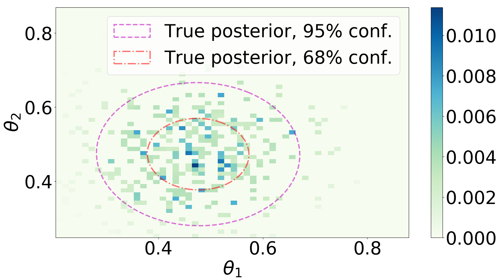
(a) $\bm{\theta}_{\ast}=(0.5,0.5)$

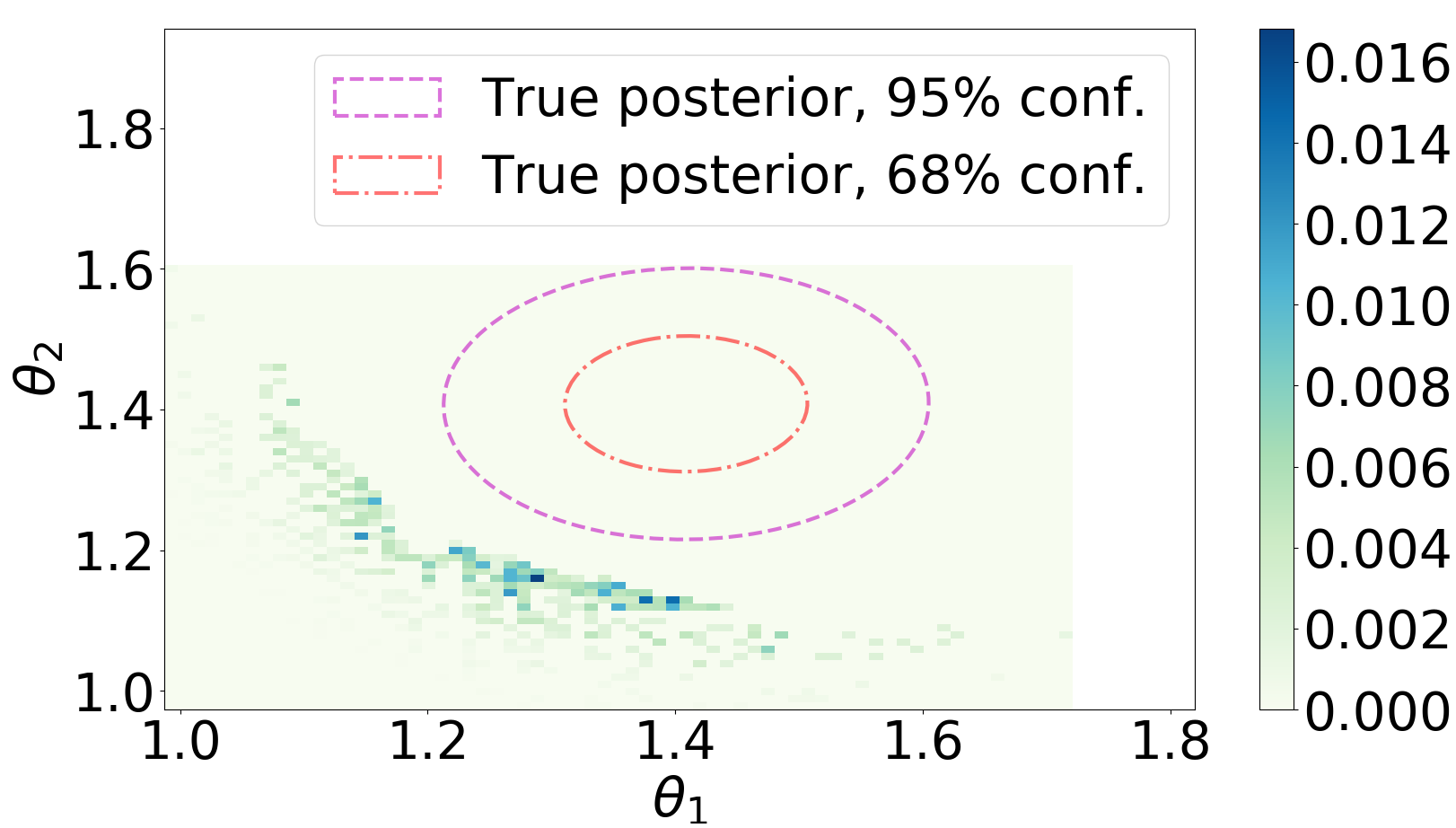
(b) $\bm{\theta}_{\ast}=(1.5,1.5)$

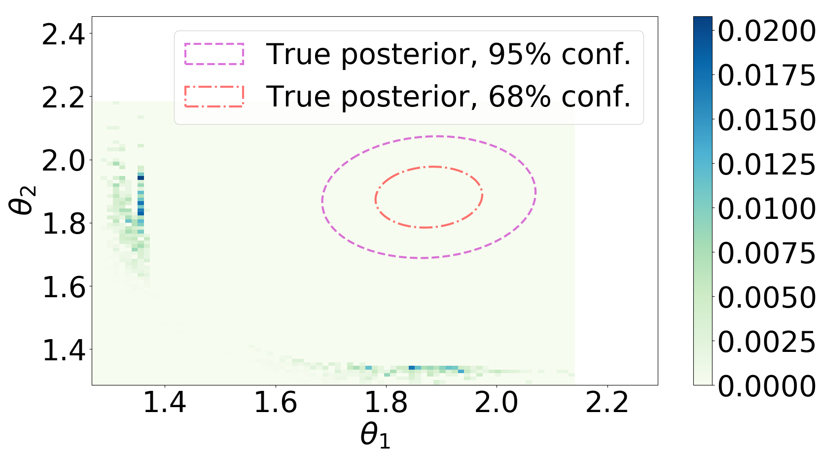
(c) $\bm{\theta}_{\ast}=(2.0,2.0)$

Figure 6: Two-dimensional histograms of MultiNest posterior samples (color scale) obtained without PR in the bivariate example, for cases (1)–(3). The colour map from light yellow to dark blue denotes low to high posterior sample density. The 68% and 95% contours of the true posterior distribution is each case are also shown.

Suppose one makes $N$ independent measurements $\mathbf{X}=[\mathbf{x}_{1},\cdots,\mathbf{x}_{n},\cdots,\mathbf{x}_{N}]^{\top}$ of some two-dimensional quantity $\bm{\theta}=(\mathbf{\mathit{\theta}}_{1},\mathbf{\mathit{\theta}}_{2})^{\top}$, such that in an analogous manner to that considered in equation (4) one has

$$\mathbf{x}_{n}=\bm{\theta}+\bm{\xi},$$ (13)

where $\bm{\xi}=(\mathit{\xi}_{1},\mathit{\xi}_{2})$ denotes the simulated measurement noise, which is Gaussian distributed $\bm{\xi}\sim\mathcal{N}(\bm{\mathit{\mu}}_{\bm{\xi}},\bm{\Sigma}_{\bm{\xi}})$ with mean $\bm{\mathit{\mu}}_{\bm{\xi}}$ and covariance matrix $\bm{\Sigma}_{\bm{\xi}}$. For simplicity, we will again assume the measurement process is unbiased, so that $\bm{\mathit{\mu}}_{\bm{\xi}}=(0,0)$, and that the covariance matrix is diagonal $\bm{\Sigma}_{\bm{\xi}}=\mbox{diag}(\sigma_{\mathit{\xi}_{1}}^{2},\sigma_{\mathit{\xi}_{2}}^{2})$, so that there is no correlation between $\mathit{\xi}_{1}$ and $\mathit{\xi}_{2}$, and the individual variances are known a priori. We also assume a bivariate Gaussian form for the prior $\bm{\theta}\sim\mathcal{N}(\bm{\mathit{\mu}}_{\bm{\theta}},\bm{\Sigma}_{\bm{\theta}})$, where $\bm{\mathit{\mu}}_{\bm{\theta}}=(0,0)$ and $\bm{\Sigma}_{\bm{\theta}}=\mbox{diag}(\sigma_{\mathbf{\mathit{\theta}}_{1}}^{2},\sigma_{\mathbf{\mathit{\theta}}_{2}}^{2})$.

We consider three cases, where the true values of the unknown parameters are, respectively, given by: (1) $\bm{\theta}_{\ast}=(0.5,0.5)$; (2) $\bm{\theta}_{\ast}=(1.5,1.5)$; and (3) $\bm{\theta}_{\ast}=(2.0,2.0)$. In each case, we assume the noise standard deviation to be $\sigma_{\mathit{\xi}_{1}}=\sigma_{\mathit{\xi}_{2}}=0.1$, and the width of the prior to be $\sigma_{\mathbf{\mathit{\theta}}_{1}}=\sigma_{\mathbf{\mathit{\theta}}_{2}}=0.4$. We assume one observation for each case, i.e., $N=1$.

In each case, the MultiNest sampling parameters were set to $N_{\rm live}=100$, ${\rm efr}=0.8$ and ${\rm tol}=0.5$ (see Feroz et al 2009 for details), and the algorithm was run to convergence. The results obtained without apply the PR method (which is equivalent to setting $\mathit{\beta}=1$) are shown in Figure 6. One sees that the MultiNest samples are consistent with the true posterior distribution for case (1), but the sampler fails in cases (2) and (3) in which the ground truth lies far into the wings of the prior.

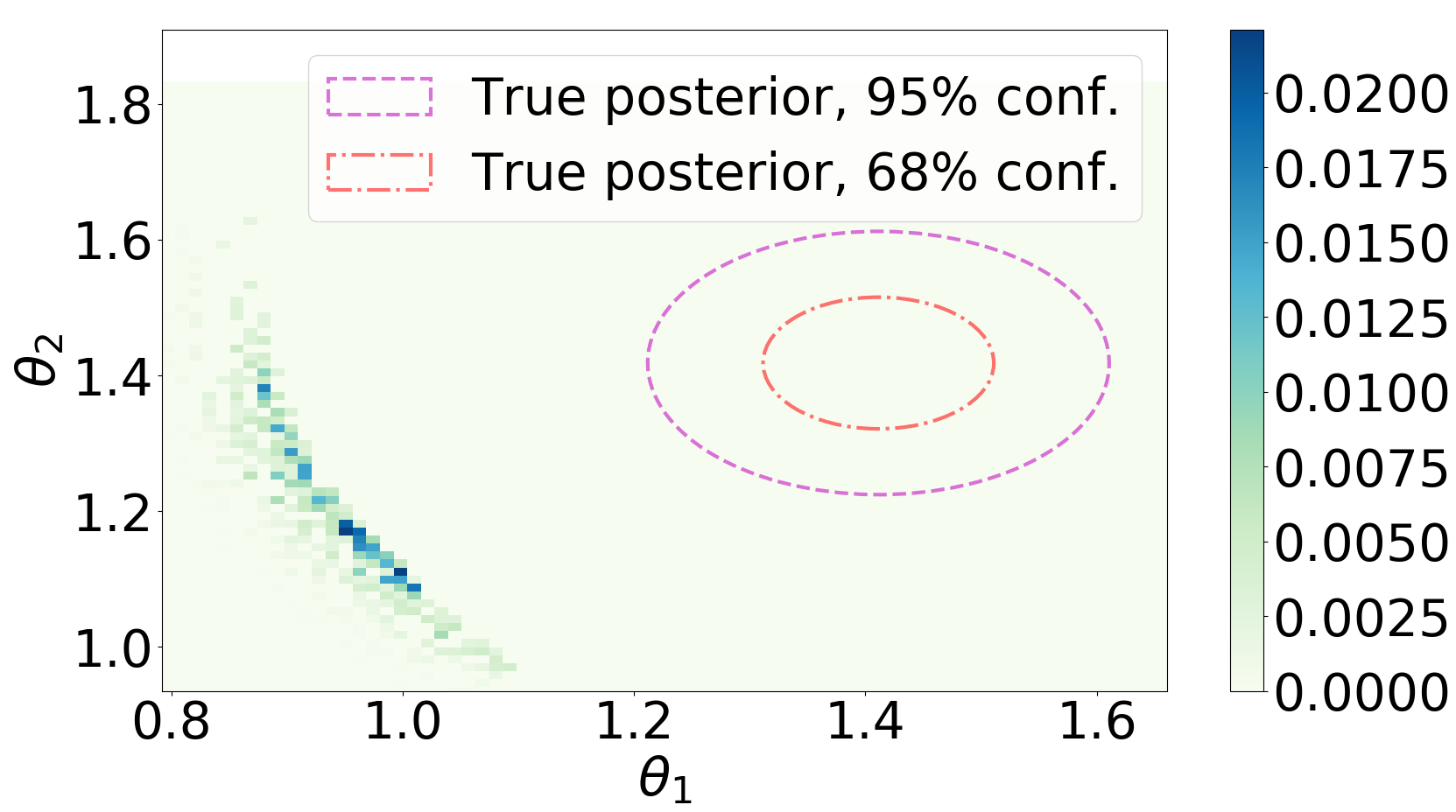
(a) case (2), $\mathit{\beta}=0.6$

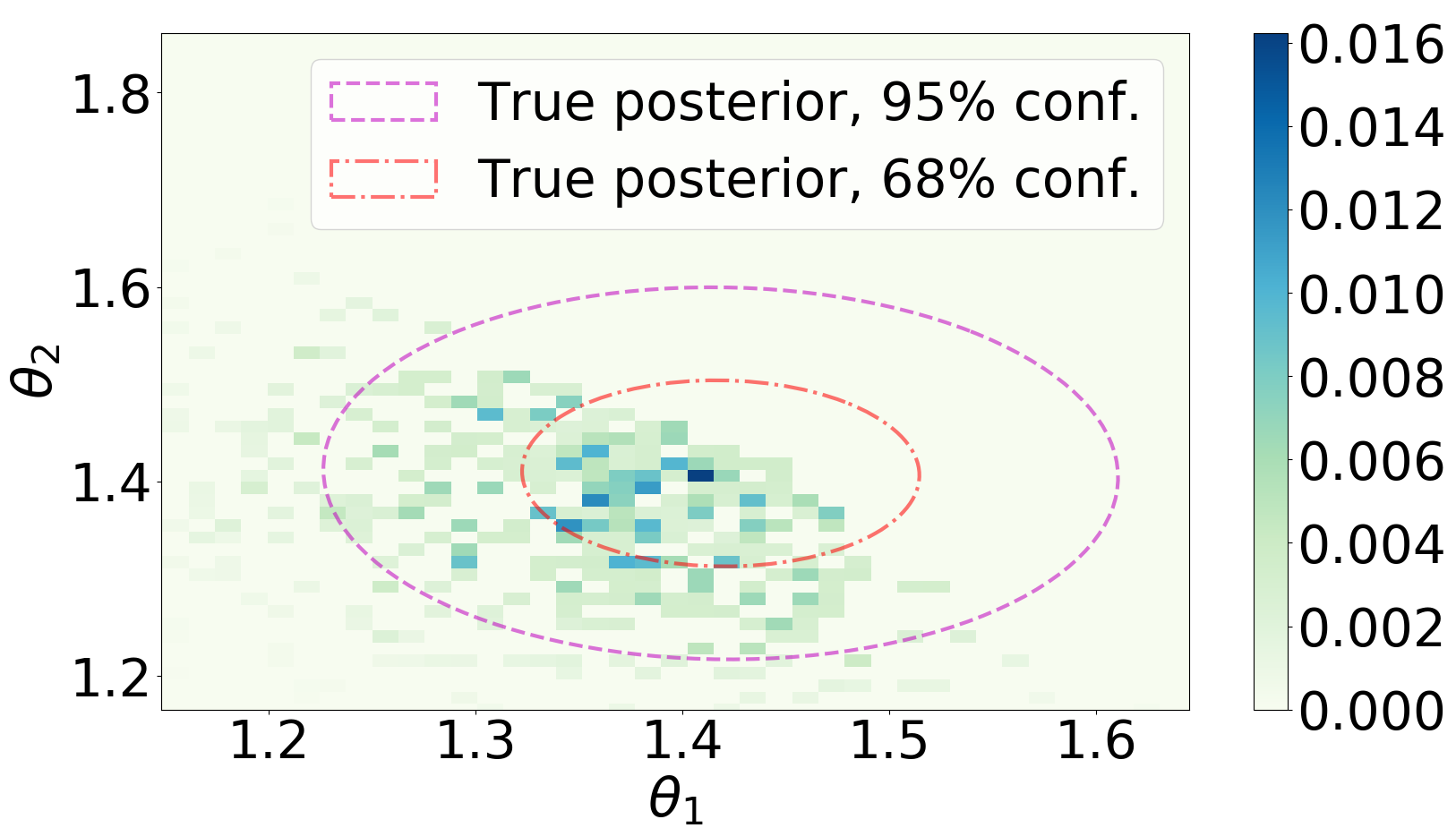
(b) case (2), $\mathit{\beta}=0.3$

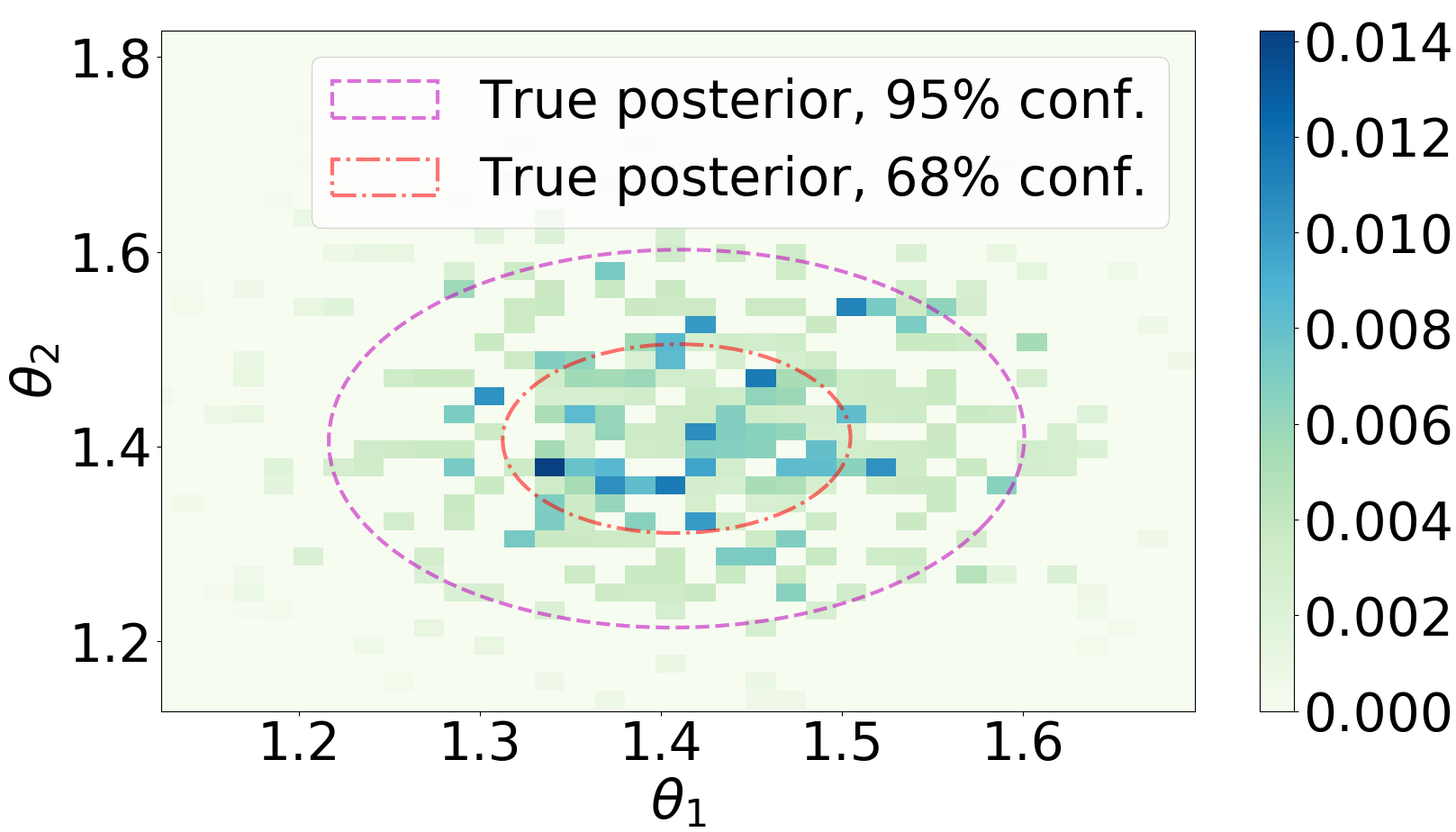
(c) case (2), $\mathit{\beta}=0.1$

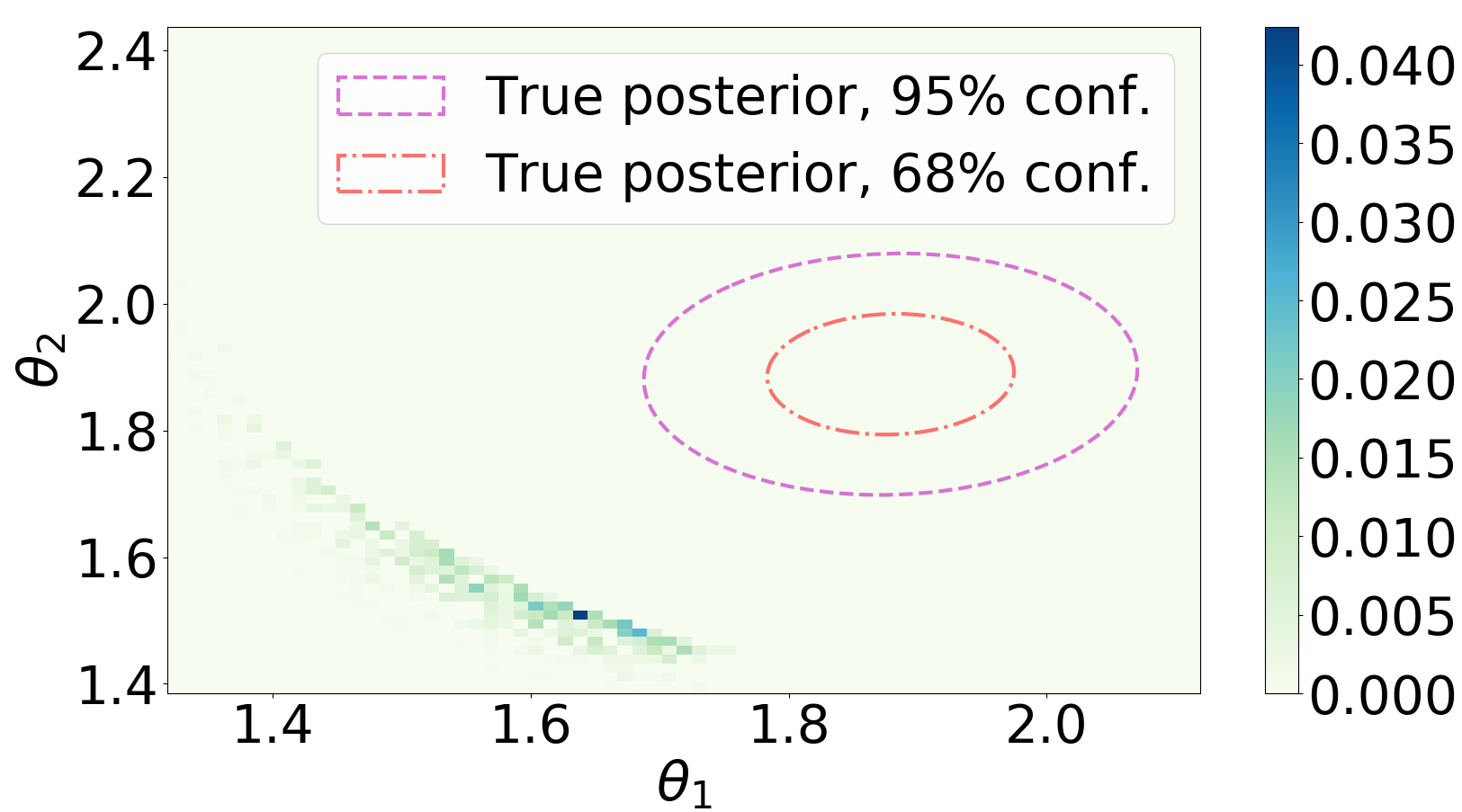
(d) case (3), $\mathit{\beta}=0.6$

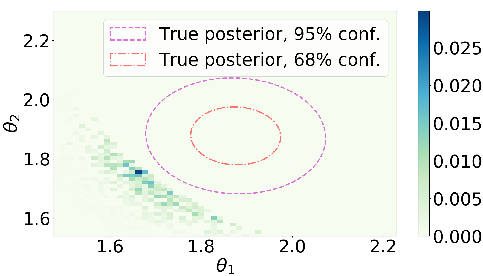
(e) case (3), $\mathit{\beta}=0.3$

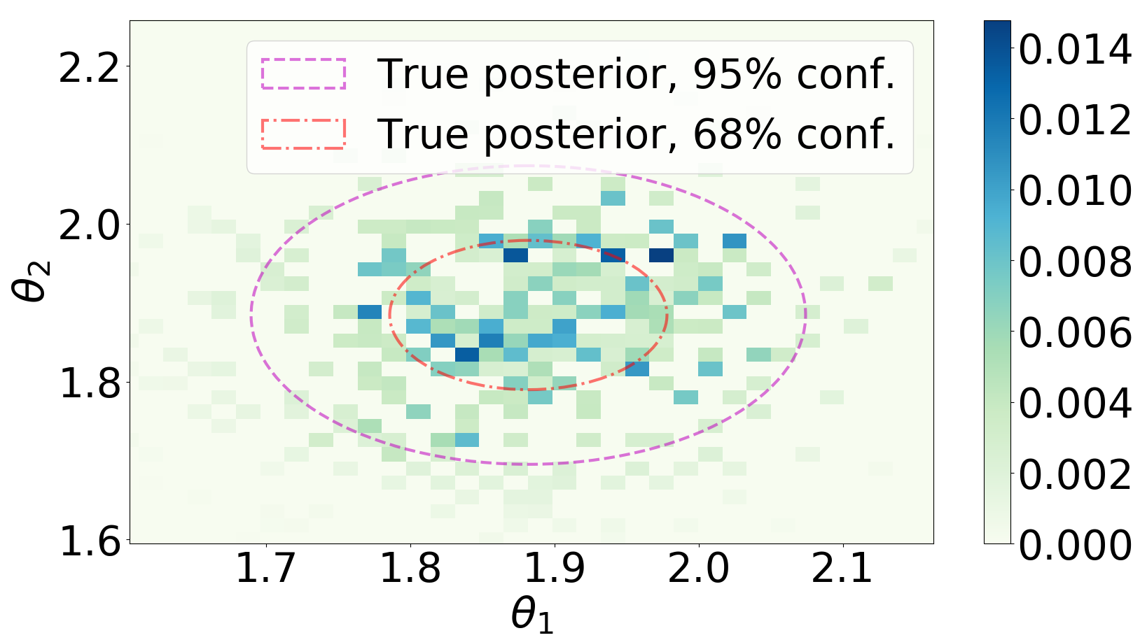
(f) case (3), $\mathit{\beta}=0.1$

Figure 7: MultiNest performance with PR method in the bivariate toy example for case (2) $\bm{\theta}_{\ast}=(1.5,1.5)$ (top four sub-figures) and case (3) $\bm{\theta}_{\ast}=(2.0,2.0)$ (bottom four sub-figures). As indicated, the panels correspond to $\mathit{\beta}$ values of 0.6, 0.3, and 0.1, respectively. The colour map from light yellow to dark blue denotes low to high posterior sample density.

Table 3: A comparison between MultiNest with and without PR method (for various values of $\mathit{\beta}$, and 100 live samples), standard MCMC algorithm (termed as ‘MCMC’), and standard importance sampling algorithm (termed as ’IS’) in the bivariate toy example for all three cases. The top half of the table is a comparison of RMSE, and the second half is for the number of likelihood evaluations ($N_{\rm like}$) per individual algorithm run. For $\mathit{\beta}=0.05$ (highlighted in bold) MultiNest achieves relatively better and consistent RMSE and $N_{\rm like}$ performance across the three cases. The number of posterior samples from the competing algorithms (MCMC and IS) are fixed to values around $1100$ in order to obtain a similar number of likelihood evaluations as required by MultiNest for $\mathit{\beta}=0.05$.

RMSE	MN ($\mathit{\beta}=1$)	$\mathit{\beta}=0.4$	$\mathit{\beta}=0.2$	$\mathit{\beta}=0.1$	$\mathit{\beta}=0.05$	$\mathit{\beta}=10^{-5}$	MCMC	IS
Case (1)	0.0066	0.0046	0.0055	0.0043	0.0038	0.0037	0.0293	0.0252
Case (2)	0.3495	0.0518	0.0117	0.0052	0.0049	0.0046	0.0797	0.4117
Case (3)	0.5586	0.3785	0.0276	0.0055	0.0045	0.0044	0.0992	0.8386
$N_{\rm like}$
Case (1)	908	847	909	959	1052	2246	1100	1100
Case (2)	2232	1553	1221	1127	1118	2271	1100	1100
Case (3)	3466	1922	1516	1280	1188	2348	1100	1100

The MultiNest posterior samples obtained using the PR method, with $\mathit{\beta}=0.6,0.3,0.1$, respectively, are shown in Figure 7 for case (2) and case (3). In each case, one sees that as $\mathit{\beta}$ decreases the samples become consistent with the true posterior. In practice, it is thus necessary to reduce the value of $\mathit{\beta}$ until the inferences converge to a sufficient accuracy.

Table 3 summarises the inference accuracy and the computational efficiency for all three cases for MultiNest without PR (which corresponds to $\beta=1$) and with PR for $\mathit{\beta}=0.4,0.2,0.1,0.05,10^{-5}$. One sees that for case (1) $\bm{\theta}_{\ast}=(0.5,0.5)$, applying PR to MultiNest has only a weak effect on the RMSE performance and the number of likelihood evaluations, with both changing by about a factor of about two (in opposite directions) across the range of $\mathit{\beta}$ values considered. For case (2) $\bm{\theta}_{\ast}=(1.5,1.5)$ and case (3) $\bm{\theta}_{\ast}=(2,2)$, however, MultiNest without PR suffers from the unrepresentative prior problem and the corresponding RMSE and number of likelihood evaluations are considerably higher than in case (1). Nonetheless, by combining MultiNest with the PR method, the RMSE and number of likelihood evaluations can be made consistent across the three cases considered. One sees that the RMSE decreases as $\mathit{\beta}$ decreases and the maximum accuracy is obtained when $\mathit{\beta}=10^{-5}$ (for which the modified prior is very close to uniform). This should be contrasted with the total number of likelihood evaluations, which increases as $\beta$ decreases. Indeed, it is clear that the minimum number of likelihood evaluations are required for intermediate values of $\mathit{\beta}$. These results show that a reasonable compromise between accuracy and computational efficiency is obtained for $\mathit{\beta}=0.05$ in this problem, which also provides the best consistency for both RMSE and the number of likelihood evaluations across all three cases.

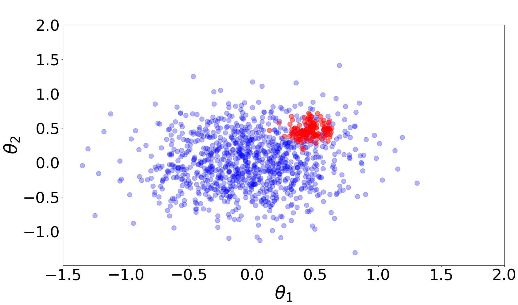
(a) case (1), KL score 169

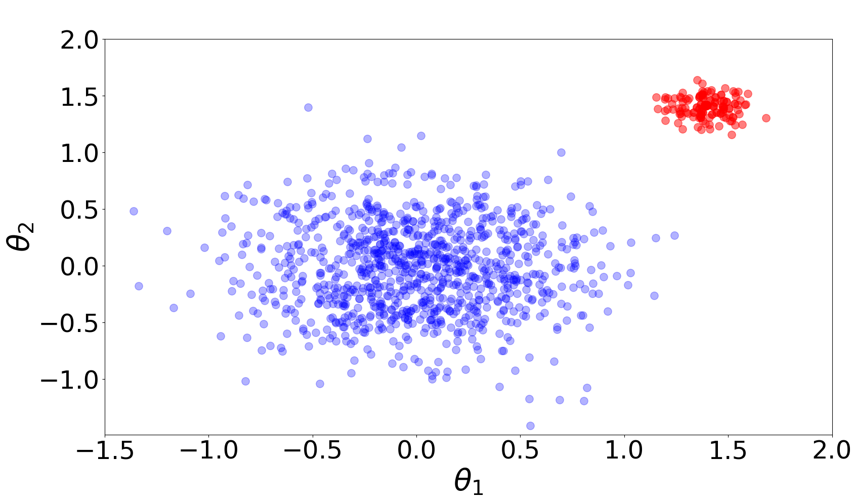
(b) case (2), KL score 1833

Figure 8: Demonstration of the KL divergence diagnostic for case (1) and case (2) in the bivariate example. The blue dots represent random samples drawn from the prior distribution, and the red dots are posterior samples from MultiNest with $\beta=0.01$ and $N_{\rm live}=100$.

5.2.1 Other sampling algorithms

Since our focus here is to introduce the PR method to improve NS performance in problems with unrepresentative priors, a full comparison between MultiNest and other competing sampling algorithms is beyond the scope of this paper. Nonetheless, we report here on some results of a brief such comparison on the same bivariate example. In particular, we perform a comparison of MultiNest with PR, in terms both of the RMSE and the number of likelihood evaluations, with our own implementation of standard MCMC sampling using the Metropolis–Hastings algorithm with a Gaussian proposal distribution and also with importance sampling (IS), using a standard IS implementation from Python package ‘pypmc’ (Jahn et al, 2018).

The results obtained using MCMC and IS are shown in the final two columns of Table 3. For $\mathit{\beta}=0.05$ MultiNest achieves relatively better and consistent RMSE and ${\rm N_{like}}$ performance across the three cases. The number of posterior samples from the competing algorithms (MCMC and IS) are fixed to values around $1100$ in order to obtain a similar number of likelihood evaluations as required by MultiNest for $\mathit{\beta}=0.05$. For case (1), the performance of IS is comparable to that of MCMC. However, in cases (2) and (3), IS is comparable to MultiNest with $\mathit{\beta}=1$, so it is clear that IS also suffers from the unrepresentative prior problem.

The detailed comparison of different sampling algorithms is a broad topic that has been widely discussed and explored in the literature. For example, importance sampling was formulated as a special case of bridge sampling, and was compared in (Gronau et al, 2017). An importance nested sampling was proposed to incorporate importance sampling into NS evidence calculation step in (Feroz et al, 2013). A comparison between NS and MCMC was discussed in (Allison and Dunkley, 2013). A review of importance sampling is presented in (Tokdar and Kass, 2010).

5.2.2 Diagnostics for bivariate example

We take the opportunity here to illustrate the diagnostics process discussed in Section 4.4 using the bivariate example. Since case (1) does not suffer from the unrepresentative prior problem, it can be treated as a reliable example and we assume that the ‘available knowledge’ is gained by analysing this case. As shown in Table 3, the number of likelihood evaluations (which is proportional to the runtime) for MultiNest without PR $(\mathit{\beta}=1)$ increases significantly from case (1) to case (3). Thus, the unrepresentative prior problem can be identified on-the-fly by monitoring the runtime. An on-the-fly convergence rate check may also be straightforwardly applied using existing rate of convergence methods (Süli and Mayers, 2003) to the problem. In either case, one may identify that case (2) and case (3) differ significantly from the available knowledge, and hence the PR method should be applied.

However, for some sampling methods, on-the-fly diagnostic of monitoring the runtime would fail in the case (adopted here) in which the number of likelihood evaluations is fixed. In this case, one must therefore rely on an after-run diagnostic, such as the KL divergence, which quantifies the differences between the assumed prior and the corresponding posterior obtained in the analysis. Figure 8 shows MultiNest samples from the prior and the posterior for case (1) and case (2), respectively, of the bivariate example. By computing the standard KL divergence, we find a value (termed KL score) of 169 for case (1) (the available knowledge) and 1833 for case (2). It is clear that the KL score for the unrepresentative prior problem is much larger than normal case, and so case (2) could be flagged as an outlier according to some predefined criterion on KL score. Similarly considerations apply to case (3).

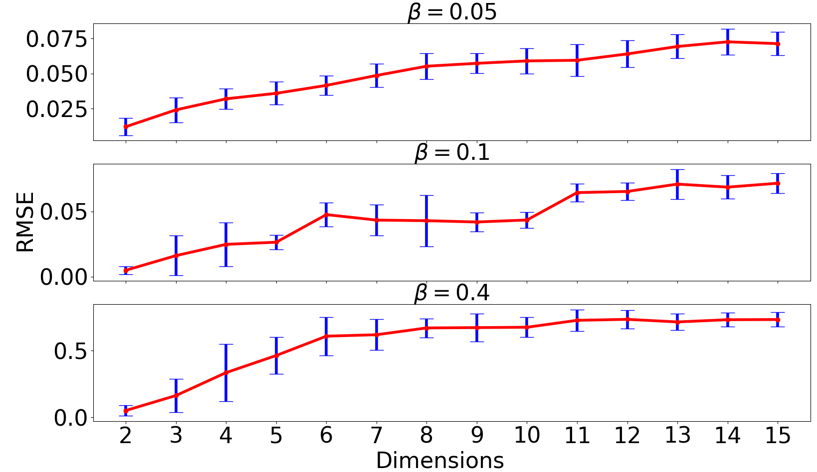
(a) RMSE

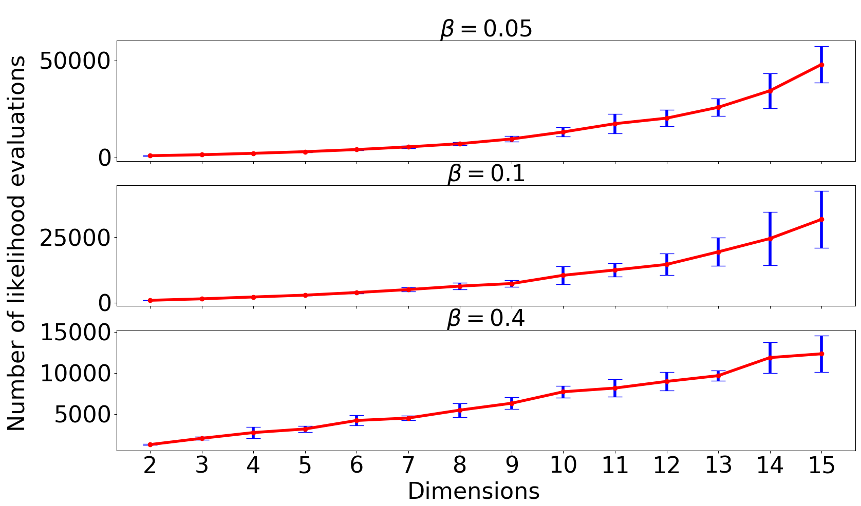
(b) Number of likelihood evaluations

Figure 9: Performance of MultiNest with the PR method applied to the case (2) bivariate toy example extended to higher dimensions. The $\mathit{\beta}$ values considered are $0.05,0.1,0.4$, from top to bottom in each subfigure, respectively. The truth for each dimension is set to a same value $\mathbf{\mathit{\theta}}_{\ast}=1.5$. The RMSE (left-hand column) and number of likelihood evaluations (right-hand column) are calculated over 20 repeated realisations with same settings as those in bivariate example case (2). The red line represents the mean value of the repeated realisations, and the blue error bar indicates the standard deviation.

5.3 Higher-dimensional examples

In order to investigate the performance of PR in higher dimensionality, we reconsider case (2) in the bivariate example, but extend the dimensionality over the range 3 to 15 dimensions. In particular, we consider the performance with $\beta=0.05,0.1$, and $0.4$. Each of the experiments is repeated 20 times, and the test results are evaluated by calculating the mean and standard deviation of the RMSE over these 20 realisations.

As shown in Figure 9 (a), with an increase of dimensionality, the RMSE error-bar undergoes an obvious increase for both $\mathit{\beta}=0.05$ and $0.1$ cases. For the case $\mathit{\beta}=0.4$, the RMSE increases at lower dimensionality, but then remains at a stable level for higher dimensionality. Overall, the RMSE performance in higher dimensions is consistent with that in the bivariate example in terms of its order of magnitude, which demonstrates that the PR method is stable and effective for problems with higher dimensionality.

Figure 9 (b) shows a set of equivalent plots for the number of likelihood evaluations. This clearly shows that for a smaller $\mathit{\beta}$ value MultiNest makes a larger number of likelihood evaluations. This is not surprising as a smaller $\mathit{\beta}$ corresponds to a broader modified prior space. We note that the number of likelihood evaluations required for $\mathit{\beta}=0.05$ is almost twice that for $\mathit{\beta}=0.1$.

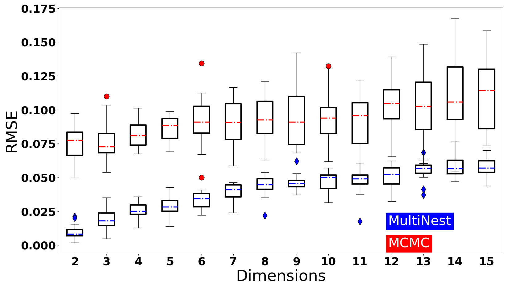
Figure 10: RMSE boxplot for high dimensionality comparison between MultiNest with the PR method (100 live samples, $\mathit{\beta}=0.05$) and MCMC for case (2) $\mathbf{\mathit{\theta}}_{\ast}=1.5$. The boxes range from the 25th to 75th quantiles. MultiNest results are in blue, and MCMC in red. The blue and red dashed lines within the box are the median RMSE over 20 realisations for each method. The blue diamond and red solid circles represent outliers among the 20 realizations. For each dimension, the two methods are computed with a comparable number of likelihood evaluations.

Figure 10 shows the RMSE comparison between MultiNest with PR $(\mathit{\beta}=0.05)$ and MCMC methods for the same higher dimensional examples. Note that the RMSE is computed using a comparable number of likelihood evaluations for the two methods for each dimensionality. As can be observed from the figure, MCMC remains stable and accurate (albeit with a slight increase in RMSE with dimension), but has a higher RMSE than MultiNest with PR across the dimensionalities considered. By contrast, for MultiNest with PR, the RMSE increases more noticably with the number of dimensions, as might be expected from a NS algorithm that is based on a form rejection sampling.

Table 4: The performance of MultiNest with and without PR method (for various values of $\mathit{\beta}$, and both 100 live samples) for all three cases of the non-Gaussian bivariate example. The top half of the table is a comparison of RMSE, and the second half is the number of likelihood evaluations ($N_{\rm like}$) per individual algorithm run. For $\mathit{\beta}=0.05$ (highlighted in bold) MultiNest achieves relatively better and consistent RMSE and $N_{\rm like}$ performance across the three cases.

RMSE	MN ($\mathit{\beta}=1$)	$\mathit{\beta}=0.4$	$\mathit{\beta}=0.2$	$\mathit{\beta}=0.1$	$\mathit{\beta}=0.05$	$\mathit{\beta}=10^{-5}$
Case (1)	0.0091	0.0085	0.0065	0.0067	0.0066	0.0055
Case (2)	0.2042	0.0655	0.0186	0.0136	0.0135	0.0125
Case (3)	0.1403	0.2057	0.0705	0.0207	0.0196	0.0191
$N_{\rm like}$
Case (1)	949	926	987	1049	1117	1313
Case (2)	2017	1356	1143	1068	1047	1151
Case (3)	2921	1337	1067	889	858	996

5.4 Non-Gaussian bivariate example

As our final numerical example, we consider a non-Gaussian bivariate likelihood function. In particular, we adapt the Gaussian bivariate likelihood considered in Section 5.2 by replacing the product of Gaussian distributions in each dimension by a product of Laplace distributions $\mbox{Laplace}(\mu,b)$, so that in each dimension the Gaussian form (5) is re-written as:

$$\mathcal{L}(\mathbf{\mathit{\theta}})=\prod_{n=1}^{N}\left\{\frac{1}{2b}\exp\left(-\frac{|\mathbf{\mathit{\theta}}-x_{n}|}{b}\right)\right\},$$ (14)

where $x_{n}$ is the $n$th measurement (although $N=1$ in this example), which acts as the location parameter similar to in a Gaussian distribution, and $b$ is the scale parameter in the Laplace distribution analogous to $\sigma_{\xi}$ in (5). We choose the Laplace distribution as our non-Gaussian test example since: (1) it is valid for both positive and negative values of the parameter $\theta$, unlike Beta/Gamma distributions; and (2) a Laplace distribution with a small $b$-value has a similar tail to that of a Gaussian (i.e. it is not heavy-tailed), which facilitates easier comparison.

The prior distribution is identical to that used Section 5.2, i.e. the same Gaussian distribution. Indeed, all of the other experimental settings are kept the same as those in Section 5.2, and we again consider MultiNest with and without PR method in all three cases.

The results of the analysis are given in Table 4 for runs with $N_{\rm live}=100$. Comparing the $N_{\rm live}=100$ results with the corresponding ones given in Table 3 for the Gaussian bivariate example, ones sees that the trends for both RMSE and $N_{\rm like}$ are similar to those in the Gaussian bivariate cases, but are in general higher for the Laplace distribution. This is because the peak of the Laplace distribution is sharper than that of a Gaussian. Again reasonable results are obtained for $\mathit{\beta}=0.05$.

Figure 11 shows the RMSE resulting from different $N_{\rm live}$ values for $\mathit{\beta}=0.05$ and $10^{-5}$, respectively. Comparing these RMSE values with those given in Table 3, which were obtained for the Gaussian bivariate example with $N_{\rm live}=100$, one sees that higher $N_{\rm live}$ values are required for the Laplace distribution to achieve similar levels of accuracy.

Figure 11: RMSE performance of MultiNest in the non-Gaussian bivariate example with different $N_{\rm live}$ and $\mathit{\beta}$ values for case (2) and (3).

6 Conclusions

This paper addresses the unrepresentative prior problem in Bayesian inference problems using NS, by introducing the posterior repartitioning method.

The key advantages of the method are that: (i) it is general in nature and can be applied to any such inference problem; (ii) it is simple to implement; and (iii) the posterior distribution is unaltered and hence so too are the inferences. The method is demonstrated in univariate and bivariate numerical examples on Gaussian posteriors, and its performance is further validated and compared with MCMC sampling methods in examples up to 15 dimensions. The method is also tested on a non-Gaussian bivariate example. In all cases, we demonstrate that NS algorithms, assisted by the PR method, can achieve accurate posterior estimation and evidence approximation in problems with an unrepresentative prior.

The proposed scheme does, however, have some limitations: (i) if the prior and likelihood are extremely widely separated, the sampling can still be inefficient and slow, because of the large augmented search space for very small $\mathit{\beta}$; (ii) the approach cannot be readily applied to problems with discrete parameters; and (iii) the normalisation of the modified prior will in general not be possible analytically, but require numerical integration.