Characterizing Ion Flows Across a Dipolarization Jet

Abstract

The structure of dipolarization jets with finite width in the dawn-dusk direction relevant to magnetic reconnection in the Earth’s magnetotail is explored with particle-in-cell simulations. We carry out Riemann simulations of the evolution of the jet in the dawn-dusk, north-south plane to investigate the dependence of the jet structure on the jet width in the dawn-dusk direction. We find that the magnetic field and Earth-directed ion flow structure depend on the dawn-dusk width. A reversal in the usual Hall magnetic field near the center of the current sheet on the dusk side of larger jets is observed. For small widths, the maximum velocity of the Earthward flow is significantly reduced below the theoretical limit of the upstream Alfvén speed. However, the ion flow speed approaches this limit once the width exceeds the ion Larmor radius based on the normal magnetic field, $B_{z}$.

Geophysical Research Letters

IREAP, University of Maryland, College Park MD 20742-3511, USA

Dependence of the structure of dipolarization jets, or reconnection exhausts, on the cross-tail width is studied through 2D simulations

For small widths, a linear relationship is found between the maximum ion outflow speed in the jet and the width of the jet

Various measurements made by satellites could indicate the relative position of the jet and/or the size of the jet

1 Introduction

Magnetic reconnection is a common phenomenon in the Earth’s magnetotail, solar flares, coronal mass ejections, and sawtooth crashes in tokamaks; as such, it is a subject of active research. When two oppositely directed field lines reconnect, energy stored in the magnetic field is transferred to particle energy (Angelopoulos et al., 2008). The particles are accelerated by the tension in the reconnected field lines in two oppositely directed jets away from the x-line, the location where the reconnecting component of the field vanishes. In the case of the magnetotail, reconnection causes one jet to move Earthward and the other to be directed tailward. While it has been shown that the Alfvén speed is the maximum speed to which these dipolarization jets can accelerate flows (Parker, 1957), it is unclear how the extent of the jet in the dawn-dusk direction affects this result.

Reconnection begins at the x-line and many studies have examined the ion and electron dissipation regions centered around it. We focus farther downstream on the structure of the dipolarization jet. Previous 2D simulations (e.g., Sitnov & Swisdak, 2011; Wu & Shay, 2012) frequently focus on the $x-z$ plane (in GSM coordinates) and have examined the snowplow-like behavior of the dipolarization front as it sweeps up plasma during its earthward motion. Such simulations implicitly assume that the dipolarization jet has infinite extent in the $y$-direction. Performing fully 3D simulations lifts this restriction. Several authors have recently performed such simulations (Drake et al., 2014; Pritchett et al., 2014; Sitnov & Swisdak, 2011; Sitnov et al., 2014, 2017). Generally speaking they find that the full dimensionality allows for more complicated dynamics and the development of structure along the jet (i.e., in the dawn-dusk direction). However, the computational cost associated with such simulations means that it is difficult to examine the parametric dependence of dipolarization jet evolution.

For example, Drake et al. (2014) studied a fully three-dimensional model and found that the center of the jet (in the $x$ direction) is fairly laminar when compared to the Earthward and tailward edges. This suggests that simulations in a two-dimensional plane (north-south and dawn-dusk) could serve as a useful proxy to fully three-dimensional results. In the present manuscript we use such simulations to explore dependence of the structure of magnetotail magnetic reconnection jets on their finite extent in the cross-tail direction and, in particular, how this determines the velocity profile of the Earthward-directed ion flow and the structure of the Hall magnetic fields in the cross-tail direction. We therefore are not addressing the physics of reconnection onset in the magnetotail and the mechanisms that control the finite extent (in $x$) of these jets.

During reconnection in the magnetotail, ions are accelerated toward the Earth and down the tail by the newly reconnected magnetic fields. To accelerate up to the Alfvén speed, they first move in the cross-tail direction, the direction of the reconnection electric field, before they turn toward or away from the Earth. It is not a surprise, therefore, that in very narrow jets the ions are unable to gain enough energy to reach the Alfvén speed. In this manuscript we quantify the relation between the peak ion Earthward flow and the cross-tail width of the jet.

That the finite cross-tail width of the jet can impact the Hall magnetic field is more surprising. It is well-known from theory, simulations and observations that Hall magnetic fields are produced near the x-line (Oieroset et al., 2001; Mandt et al., 1994; Sonnerup, 1979). These fields arise because they are primarily frozen-in to the electrons inside of the ion diffusion region. Thus the electrons, which are carrying the current in the current sheet, enter the ion diffusion region and push on the fields, bending the reconnection magnetic field into the out-of-plane direction. Simulations indicate that these Hall fields are carried far downstream, $\sim 100d_{i}$, from the x-line (Le et al., 2010; Shay et al., 2011), especially away from the center of the current sheet. We find that the Hall fields reverse inside of the current sheet for large widths in the dawn-dusk direction. However, these fields do return to the expected orientation away from the current sheet. This effect is due to the ions from the current sheet becoming frozen-in to the magnetic fields of the jet, and thus pushing on the fields in the opposite direction of the electrons.

2 Simulations

We use the particle-in-cell code p3d (Zeiler et al., 2002). The magnetic field strength $B_{0}$ and density $n_{0}$ define the Alfvén speed $V_{A}=\sqrt{B_{0}^{2}/4\pi m_{i}n_{0}}$, with lengths normalized to the ion inertial length $d_{i}=c/\omega_{pi}$, where $\omega_{pi}$ is the ion plasma frequency, and times to the ion cyclotron time $\Omega_{i0}^{-1}$. Electric fields and temperatures are normalized to $V_{A}B_{0}/c$ and $m_{i}V_{A}^{2}$, respectively. The coordinate system for all simulations is Geocentric Solar Magnetospheric (GSM).

The initial conditions for the simulations are intended to mimic those of a dipolarization jet. We start with a classical Harris current sheet with an asymptotic magnetic field $B_{0}$, central density $n_{0}$ and uniform background density $n_{b}=0.3n_{0}$. To this equilibrium, we add a constant $B_{z}$ that is localized in the dawn-dusk ($y$) direction with a corresponding plasma density equal to the lobe density, $n_{b}$. The intent is to depict late-time tail reconnection in which the jet is formed from heated lobe plasma. Hence, in the region with $B_{z}$ non-zero, the field is non-zero at the symmetry (equatorial) plane. In order to maintain pressure balance we modify the electron and ion temperatures in the jet. The temperatures elsewhere, in code units, are 1/12 and 5/12 for the electrons and ions respectively. The ion-to-electron mass ratio is set to 25, which is sufficient to separate the electron and ion scales. All the forces are balanced in the $y$ and $z$ directions but there is an unbalanced force in the $x$ direction due to a non zero $B_{z}\partial_{z}B_{x}$ term in the fluid momentum equation. This force accelerates the plasma towards the Earth in the magnetotail. Following initialization the system adjusts and reaches a quasi-steady configuration as in a conventional Riemann model.

We perform quasi-two-dimensional (quasi-2D) simulations with two full spatial dimensions ($y$ and $z$) and one ($x$) with small extent. To mitigate the resulting noise, our analysis of employs averages over all cells in the $x$ direction. These computationally cheap simulations allow us to explore jets of different widths at late times. Typical simulation dimensions are $(x,y,z)=(3.2,102.4,102.4)d_{i}$. We also examine a more expensive simulation with $(x,y,z)=(102.4,25.6,25.6)d_{i}$, which has already been discussed in Drake et al. (2014). The spatial grid has a resolution $\Delta=0.05$ while the smallest physical scale is the Debye length in the magnetotail, $\approx 0.03$. We use $100$ particles per cell per species for the simulations with a small extent in $x$. The simulation with a larger extent in $x$ uses $50$ particles per cell. In all simulations the speed of light is $c=15$ and we employ periodic boundary conditions in all directions. (Note that periodicity in $z$ actually requires us to simulate two mirror-image current sheets. We stop the simulation before the two current sheets begin to interact and only present results from one. Both sheets undergo very similar evolution.) The widths, $w$, we examine are: $\sim 1d_{i}$, $\sim 2d_{i}$, $\sim 3d_{i}$, $\sim 4d_{i}$, $\sim 7d_{i}$, $\sim 15d_{i}$, $\sim 30d_{i}$, and infinite (occupying the full space along $y$). For a full comparison between the quasi-2D simulations and the full 3D version see the supporting information.

3 Presentation and analysis of simulation results

3.1 Reversal of the Hall Field

As a result of the system’s evolution, the Hall magnetic field ($B_{y}$) on the dawn edge of the jet reverses sign from its usual direction, especially for jets with a large width. Figure 1 is an image of the total current in the $x$ direction for the simulation with the largest finite-width dipolarization jet, $w\sim 30d_{i}$. Overlaid are arrows showing the in-plane ion flows and magnetic field lines in shades of green. The current layer can be identified by the ions flowing duskward ($-2\leq z/d_{i}\leq 2$). The electrons (not shown) flow dawnward within the current sheet. The ends of the field lines are evenly distributed along the bottom of the jet in $z$ and followed until they leave the area depicted in Figure 1. Below the 2D image is a cut through the center of the current sheet of the ion current in the $y$ direction.

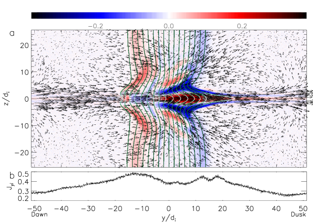
Figure 1: Panel (a) is the $x$ component of the total current in the $y-z$ plane at $\Omega_{i0}t=40$. Plotted in black arrows are ion flow vectors with the length proportional to the magnitude of the velocity. The in-plane magnetic field lines in the jet are displayed in green, with darker shades indicating a stronger magnetic field. Panel (b) is a cut of the total ion current in the $y$ direction through the center of the current sheet ($z/d_{i}=0$).

On the dawn (left) side of the jet the electrons carry the magnetic field to the left and produce the usual sign of the Hall magnetic field $B_{y}$ (negative below the center of the current sheet and positive above). The small dimple on the extreme dawn edge is likely due to ions carrying the field towards the dusk.

On the dusk (right) side of the jet, however, $B_{y}$ reverses sign compared with the usual Hall magnetic field, as is visible above and below the center of the current sheet in Figure 1. The reversal in this case arises due to ions pushing on the field as a result of the vortex pair that forms just duskward of the jet. The vortex pair consists of two adjacent vortices that are centered just above and below the current layer. Their vorticity has opposite signs so their flows add at the center of the current layer. The resulting strong duskward ion flow near the center of the current sheet carries the field lines toward the dusk while the return (dawnward) ion flow above and below the current sheet carries the field lines toward the dawn. The result is a reversal in the Hall field just above and below the center of the current sheet with the sign of $B_{y}$ taking the usual values further away from the current sheet.

We now discuss the mechanism for the development of the vortex pair. In the initial state the ions flow uniformly across the domain toward the dusk. The imposed $B_{z}$ diverts the flowing ions toward the Earth, which slows their duskward flow. The flowing ions outside of the jet on the dusk side continue to flow toward the dusk and try to fill in this depletion by turning back toward the jet, thereby forming the two vortices evident in Figure 1(a). The reduction of the ion current shown in the cut along the middle of the current layer in Figure 1(b) over the interval $20<y/d_{i}<40$ results from the diversion of the ion flow away from the current layer as seen in the velocity vectors of Figure 1(a).

The ions in the jet contribute to closing these ion vortices. As time progresses, the tension in the ”reconnected” magnetic field (in the $z-x$ plane) drives the plasma flow in the positive $x$ (earthward) direction. This motion causes ions in the lobes to move towards the current sheet and produces the converging flows (toward $z=0$) seen on the duskward edge of the jet. Upon entering the current sheet, the ions move in Speiser-like orbits and rotate first into the positive $y$ direction before completing their Speiser motion into Earthward flow. Their motion in the duskward direction as they rotate in the current layer contributes to the enhancement in $J_{iy}$ seen around $y/d_{i}\sim 15$ in Figure 1(b). This high-speed ion flow carries the magnetic field duskward and drives the reversed Hall field seen in the data.

An organized reversal in the Hall magnetic field has not been seen even in large-scale 2D reconnection simulations (carried out in the $x$-$z$ plane) (Le et al., 2010; Shay et al., 2011) although firehose-driven turbulence in the jet can produce local reversals of $B_{y}$ (Hietala et al., 2015). An important question then is whether these earlier results are consistent with the Hall field reversal seen in the present simulations with the largest jet width. Since nearly all of the ions in dipolarization jets originates upstream in the lobes, they carry little cross-tail momentum as they enter the jet and total momentum conservation in the cross-tail direction means that they will not gain a significant net flow in the cross-tail direction (Liu et al., 2012), it is therefore the electrons that carry most of the cross-tail current in 2D reconnection simulations. An infinite width jet would, of course, not produce the vortex shown in Fig. 1(a) since $\partial_{y}=0$. Thus, we would not expect the Hall field to reverse for jets with infinite extent in the cross-tail direction. To confirm this, we performed a separate simulation with an infinite jet with only the electrons carrying the initial current. At late times there was a non-zero duskward flow of ions, but it was significantly smaller than the ion flow depicted in Figure 1 and was unable to reverse the Hall field. This result is consistent with past 2D reconnection simulations that did not see a reversal of the Hall field.

3.2 The dependence of the Earthward-directed flow on Cross-tail Width

Figure 2 shows the Earthward-directed ion flow velocity in black through the center of the current sheet ($z/d_{i}=0$) for jets with widths of $\sim 1d_{i}$, $\sim 15d_{i}$, and $\sim 30d_{i}$. For clarity, the magnetic field profile is also shown in red. For panels (b) and (c) the local $\mathbf{E}\bm{\times}\mathbf{B}$ drift velocity is also plotted in green (we neglect this for panel (a) since it is too noisy). Though not shown, the reconnection electric field $E_{y}=V_{E\times B}B_{z}$ follows the profile of $V_{E\times B}$ because $B_{z}$ is nearly constant within the jet. Panel (c) clearly shows the four phases of the ion outflow along the cross-tail direction, $y$. First, the ions enter the dawnward side of the jet with no flow in the $x$ direction. Second, upon entering the jet, the ions accelerate along the reconnection electric field $E_{y}$, which increases with distance into the jet, and rotate into the $x$ or $\mathbf{E}\bm{\times}\mathbf{B}$ drift direction. Third, their Earthward flow plateaus until they exit the jet. In the fourth phase the ions retain their x-directed motion outside of the jet since they are moving along the unreconnected magnetic field $B_{x}$. Outside of the jet, the ions mix with the background population so that the outflow speed slowly decays with increasing distance from the jet. Note that, although only the simulation shown in panel (c) with $w=30d_{i}$ is sufficiently large enough to exhibit the plateau, all three simulations produce an Earthward-directed, magnetic-field-aligned beam of ions in a region with $B_{z}=0$.

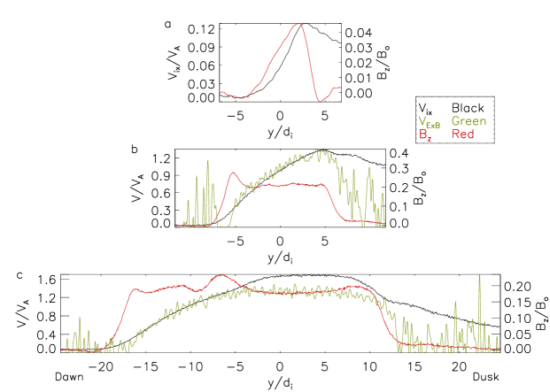
Figure 2: The $x$ component of the ion velocity (black) and the $z$ component of the magnetic field (red) from three runs at $\Omega_{i0}t=40$ along a cut taken at $z=0$. (b) and (c) also include the local $\mathbf{E}\bm{\times}\mathbf{B}$ velocity in the x direction (green). In (a) the smallest jet, width $\sim 1d_{i}$, in (b) a medium sized jet, width $\sim 15d_{i}$, and in (c) the largest finite jet, width $\sim 30d_{i}$. The images only show a portion of the full simulated space. Note that the smallest jet has significantly increased in width at late times, but that there is a corresponding decrease in the magnetic field to compensate. For this reason the $\mathbf{E}\bm{\times}\mathbf{B}$ velocity is too noisy to be seen and thus we have omitted it from this figure.

To understand the scale length of the region where the ions are accelerating, consider that the ion outflow speed plateaus at the upstream Alfvén speed. Thus we can make the following scaling argument starting with the steady state ion conservation of momentum equation for a 2D system ($\partial_{x}=0$) at $z=0$:

$$mnv_{yi}\partial_{y}v_{xi}\approx\frac{B_{z}}{4\pi}\partial_{z}B_{x}\sim mnv_{yi}\frac{C_{A}}{L_{y}}\sim\frac{B_{z}}{4\pi}\frac{B_{x}}{\Delta}$$ (1)

where $C_{A}$ is the upstream Alfvén speed, $L_{y}$ is the acceleration length scale, $\Delta$ is the half width of the current sheet, and $v_{zi}=0$ due to the symmetry of the configuration. We neglect the divergence of the pressure since it is smaller than the magnetic tension in the region of interest. Next, since the ions carry most of the current on their entry into the jet, we can approximate $v_{y}$ from Ampére’s law on the dawnside of the jet:

$$\partial_{z}B_{x}=\frac{4\pi}{c}nqv_{yi}\sim B_{x}/\Delta$$ (2)

Then, plugging $v_{y}$ into Equation 1, solving for $L_{y}$ and normalizing to code units we obtain:

$$L_{y}/d_{i}\sim\sqrt[]{\frac{n_{0}}{n_{b}}}\frac{B_{x}}{B_{z}}$$ (3)

where $n_{b}$ is the upstream ion density. For our simulation, $n_{b}/n_{0}\approx 0.3$ and $B_{x}/B_{z}\approx 5$ giving $L_{y}/d_{i}\sim 10$ which is in agreement with Figure 2 panel (c) and explains why panel (b), which only has a width of approximately $10d_{i}$, has no plateau.

While the $\mathbf{E}\bm{\times}\mathbf{B}$ drift describes the motion of the ions for medium sized and smaller jets (e.g., Fig. 2(b)), it falls short of accurately depicting the ion motion for larger jets after they plateau in speed. Thus, it is of interest to evaluate whether the particle motion within a dipolarization jet can be described by the usual guiding center drift. A quantitative test comes from evaluating the $\kappa$ parameter of Buchner and Zelenyi (1989). Defined as $\kappa=\sqrt{R_{\text{min}}/\rho_{\text{max}}}$, where $R_{\text{min}}$ is the minimum radius of curvature and $\rho_{\text{max}}$ is a particle’s maximum Larmor radius. Values greater than unity are associated with well-behaved trajectories (i.e., well-described by drifts). For our simulations we find $\kappa$ for the ions to be $\lesssim 1$ within the jets. Thus, we cannot expect the guiding center drifts to accurately describe the observed flows seen in Figure 2. Nevertheless, the underlying physics driving the drifts (curvature of the magnetic field, magnetic field gradients, etc.) will still influence the particle flows.

Although there is some agreement between the $\mathbf{E}\bm{\times}\mathbf{B}$ drift and the ion flow, there must be additional physics at work in the region where they diverge (e.g., for $-15\leq y/d_{i}\leq-5$ in panel (c)). The curvature of the magnetic field within the jet is a likely source. Recall from Figure 1 that the Hall field reverses around $y/di\sim-3$ creating field lines bent duskward. This is also where the ion flow diverges from the $\mathbf{E}\bm{\times}\mathbf{B}$ drift indicating that the curvature of the magnetic field boosts the ion flow in the $x$ direction. Direct calculation of the curvature drift leads to ion flow velocities significantly larger than observed (although of the correct sign). However, because $\kappa\lesssim 1$, the particle orbits are not well-described by drifts superimposed on circular Larmor orbits and agreement should not be expected.

It should be noted that although the jet in panel (b) has a width $\sim 2$ times greater than that of panel (a) at the time shown, the jet widths at $t=0$ differed by a factor of $\sim 15$. The widening of the jet in panel (a) is accompanied by a drop in $B_{z}$, so that the integrated magnetic flux is constant. Once the simulation begins, the electrons, as the less massive species, interact with the fields first. The electrons in the region inside of the jet initially have a large velocity in the dawn direction and a low density compared to the electrons in the current sheet outside of the jet. Hence the electrons in the jet carry the magnetic flux $B_{z}$ in the jet toward the dawn, while the electrons entering the jet from the dusk carry the flux with a lower velocity. The resulting divergence of the cross-tail electron flow spreads the flux as seen in Fig. 2(a) and leads to a build-up of magnetic flux on the dawn (left) side for larger jets. This effect leads to the smallest initial-width jet achieving a width comparable to the medium sized jet (panels a and b in Figure 2).

3.3 Maximum Ion Flow Dependence on Jet Width

It is well known that the ion flow in a dipolarization jet can be accelerated to the upstream Alfvén speed in a jet that has infinite cross-tail width. For the case of a finite width, jet we have shown that there is a transition between the nearly zero ion flow outside of the jet on the dawn side and where the flow reaches the maximum outflow speed. An ion in the current sheet enters a region of non-zero $B_{z}$ and $E_{y}$ from the dawn side and gains an $\mathbf{E}\bm{\times}\mathbf{B}$ drift in the $x$ direction. It is reasonable to expect that jets with a width less than the ion Larmor radius in the magnetic field, $B_{z}$, would be unable to fully accelerate the ions to this maximum speed since they would leave the jet before completing a full orbit. In our simulations the ions have a local Larmor radius of $\sim 5d_{i}$ (due to $B_{z}$) in the center of the jet. We start from Equation 1. Since the jet widths are short, the ion velocity $v_{yi}$ inside the jet is nearly unchanged from that outside so $v_{yi}$ is again given in Equation 2. The resulting equation for $v_{xi}$ is as follows:

$$mn\left(\frac{c\partial_{z}B_{x}}{4\pi nq}\right)\partial_{y}v_{xi}\approx\frac{B_{z}}{4\pi}\partial_{z}B_{x}\sim mn\left(\frac{cB_{x}}{4\pi nq\Delta}\right)\frac{\partial v_{xi}}{\partial y}\sim\frac{B_{z}B_{x}}{4\pi\Delta},$$ (4)

where $\Delta$ is the half width of the current sheet. The equation can be integrated to obtain the increase in $v_{xi}$ with distance inside of the jet. However, the integral is complicated by the fact that $B_{z}$ spreads in time as shown in Fig. 2. Fortunately, the total magnetic flux associated with $B_{z}$ is a constant and is given by $B_{z0}w$, where $B_{z0}$ is the initial value of $B_{z}$. Completing the integral, we obtain the maximum ion flow speed inside the dipolarization jet $v_{xi,max}$. In normalized code units the result is given by

$$v_{xi,max}/V_{A}\sim\frac{B_{z0}}{B_{x}}w/d_{i}$$ (5)

Figure 3: The $x$ component of the maximum ion flow velocity inside the jet versus the width. The linear fit shown in this figure (solid) was calculated from the first four data points. Widths greater than the local Larmor radius (dashed), $\sim 5d_{i}$, are no longer linear.

Taking values from the simulations for $B_{z}(=0.2)$, and $B_{x}(=1)$, we arrive at a slope of 0.2 for $v_{xi,max}/V_{A}$ versus $w/d_{i}$. Figure 3 shows the relationship between the maximum outflow velocity and the width $w$. A linear fit to the first few data points gives a slope of $\sim 0.12$ which differs by less than a factor of $2$ from our simple model. At larger widths, the jet velocity approaches the upstream Alfvén speed with increasing $w$. The simulation results deviate from the linear relationship for the simulation with $w=7d_{i}$, suggesting that other physical effects become important around this length scale. This is expected since the data from $w=4d_{i}$ and $w=7d_{i}$ bracket the local ion Larmor radius of $5d_{i}$ in the jet (i.e. bracket the length scale at which we expect our model to break down). For $w$ well above $\sim 5d_{i}$ the maximum $v_{ix}$ then approaches the upstream Alfvén speed, $\sim 1.8V_{A}$. Figure 3 clearly shows the strong dependence of the speed of the flow on the width of the jet.

4 Conclusion

We use quasi-2D particle-in-cell simulations to analyze the structure of the ion outflow and magnetic field on the dawn-dusk width of a dipolarization jet. For large, finite widths there is a significant reversal in the Hall magnetic field on the dusk side of the jet. This reversal, which should be detectable by spacecraft observations, results from the interaction of duskward moving ions with the magnetic field and results in the generation of a $y$ component of the magnetic field. The reversal happens approximately where the $x$-component of the ion flow reaches a maximum inside the jet and is supported by vortices above and below the current sheet that extend outside of the jet on the dusk side. The reversal of the Hall magnetic field does not appear for jets that have infinite extent in the cross-tail direction, which is consistent with simulations of symmetric reconnection that reveal Hall magnetic fields of the normal sign far downstream from the x-line (Le et al., 2010; Shay et al., 2011) and simulations that do not show any coherent behavior near the current sheet (Hietala et al., 2015). The bent field lines shown in our simulations are due to the ions moving with high velocity in the dusk direction bending the magnetic field $B_{z}$ into the cross-tail direction. This behavior does not appear in 2D models of reconnection because the ions initially in the current sheet and which carry large momentum in the cross-tail direction are swept downstream in a plasmoid (Arzner & Scholer, 2001) leaving only a population of ions from the lobes inside the jet. These ions are unable to interact with the current sheet and form a flow with a high enough cross-tail speed to reverse the Hall field.

In addition, we were able to demonstrate that there is a strong dependence of the maximum Earthward flow on the width of a dipolarization jet in the dawn-dusk direction. For jets smaller than the local Larmor radius in the reconnected magnetic field $B_{z}$ there is a linear relationship between the width of the jet and the maximum ion outflow velocity inside the jet. At larger widths, the maximum ion outflow velocity then approaches the upstream Alfvén speed. A scaling argument in support of this linear relationship suggests that the slope only depends on the ratio of $B_{z}$ to the upstream $B_{x}$.

The results of this paper could be used to establish the relative positions of satellites with respect to a dipolarization jet as well as placing limits on the cross-tail width of the jet. If the ion flow in the $x$ direction is faster than the local $\mathbf{E}\bm{\times}\mathbf{B}$ drift, especially in the presence of a reversal in the usual Hall field, the satellite must be on the dusk side of the jet and the width must be larger than the scale length $L_{y}/d_{i}=\sqrt{n_{0}/n_{u}}(B_{x}/B_{z})$. Alternatively, if an ion flow in the $x$ direction is observed without a finite $B_{z}$, that would indicate a position duskward of a dipolarization jet. A measured jet outflow velocity well below the upstream Alfvén speed and with $B_{z}\neq 0$ would suggest that the satellite is on the dawnward side of the jet or that the jet has a very small cross-tail width compared with the effective scale length $L_{y}/d_{i}=\sqrt{n_{0}/n_{u}}(B_{x}/B_{z})$.