A Candidate Tidal Disruption Event in a Quasar at $z=2.359$ from Abundance Ratio Variability

Abstract

A small fraction of quasars show an unusually high nitrogen-to-carbon ratio (N/C) in their spectra. These “nitrogen-rich” (N-rich) quasars are a long-standing puzzle because their interstellar medium implies stellar populations with abnormally high metallicities. It has recently been proposed that N-rich quasars may result from tidal disruption events (TDEs) of stars by supermassive black holes. The rapid enhancement of nitrogen and the depletion of carbon due to the carbon–nitrogen–oxygen cycle in supersolar mass stars could naturally produce high N/C. However, the TDE hypothesis predicts that the N/C should change with time, which has never hitherto been observed. Here we report the discovery of the first N-rich quasar with rapid N/C variability that could be caused by a TDE. Two spectra separated by 1.7 years (rest-frame) show that the N III] $\lambda$1750/C III] $\lambda$1909 intensity ratio decayed by $\sim 86$%$\pm$14% (1$\sigma$). Optical (rest-frame UV) light-curve and X-ray observations are qualitatively consistent with the TDE hypothesis; though, the time baseline falls short of a definitive proof. Putting the single-object discovery into context, statistical analyses of the $\sim 80$ known N-rich quasars with high-quality archival spectra show evidence (at a 5$\sigma$ significance level) of a decrease in N/C on timescales of $>1$ year (rest-frame) and a constant level of ionization (indicated by the C III] $\lambda$1909/C IV $\lambda$1549 intensity ratio). If confirmed, our results demonstrate the method of identifying TDE candidates in quasars via abundance ratio variability, opening a new window of TDE observations at high redshift ($z>2$) with upcoming large-scale time-domain spectroscopic surveys.

1 Introduction

Studies of the optical (rest-frame UV) spectra of high-redshift ($z>2$) quasars show that $\lesssim$1% exhibit much stronger nitrogen emission (seen in N V $\lambda$1240, N IV] $\lambda$1486, and/or N III] $\lambda$1750) compared to the collisionally excited lines of other heavy elements such as carbon (Bentz & Osmer, 2004; Bentz et al., 2004; Jiang et al., 2008; Batra & Baldwin, 2014). The high N/C is caused by significantly elevated nitrogen-to-carbon abundance ratios (e.g., by a factor of 10 in the prototypical case of Q0353$-$383) since physical conditions in the emission-line regions of N-rich quasars appear similar to ordinary quasars (Shields, 1976). The origin of N-rich quasars is generally attributed to unusually high metallicities (e.g., $Z>5Z_{\odot}$; Dietrich et al., 2003; Nagao et al., 2006). The high metallicities could result from either extreme global enrichment in the cores of giant elliptical galaxies (Hamann & Ferland, 1993, but see Friaca & Terlevich 1998; Romano et al. 2002 for arguments against this) or local enrichment in the central part of the quasar (Collin & Zahn, 1999; Wang et al., 2011). However, it is difficult to generate a stellar population that has elevated nitrogen abundances unless the absolute metallicity is extremely high.

TDEs have recently been proposed as an alternative, more natural explanation of the high N/C (Kochanek, 2016a). The requirement for unusually high metallicities is obviated since the N-rich phenomenon would be transient. The TDE population that may cause significant abundance anomalies would be dominated by supersolar mass stars since more massive stars are too rare and less massive stars would not have enough time for nuclear processing within the age of the universe. Although such events are expected to be rare (e.g., $\sim$10% of all TDEs), they could quickly increase N/C by factors of 3–10 (Kochanek, 2016a; Gallegos-Garcia et al., 2018). The disruption of even a single star could be enough to temporarily pollute the broad-line region (BLR) gas, assuming the BLR gas mass is on the order of $\gtrsim 10^{-3}M_{\odot}$ (Peterson, 1997). Although significant differences exist between the rest-frame UV spectra of low-redshift TDEs and high-redshift N-rich quasars, unusually strong nitrogen emission is seen in all of the three optical TDEs that have UV spectra in low-redshift galaxies (Cenko et al., 2016; Yang et al., 2017; Brown et al., 2018).

To test the TDE hypothesis, we study the spectroscopic variability for a sample of 82 N-rich quasars compiled from the literature (Jiang et al., 2008; Batra & Baldwin, 2014) that have high-quality (S/N$>10$ pixel^-1 in the spectral region of interest) archival spectra from the SDSS (York et al., 2000) and SDSS-III/BOSS (Dawson et al., 2013) surveys. Our main findings include:

1. Discovery of an $\sim 86$%$\pm$14% (1$\sigma$) weakening of the N III] $\lambda$1750/C III] $\lambda$1909 emission-line intensity ratio between 2005 and 2011 in a N-rich quasar. This is the most dramatic spectral change that has been observed in any N-rich quasar.

2. Demonstration that the observations of the decrease of the N III] $\lambda$1750/C III] $\lambda$1909 emission-line intensity ratio can be explained by a TDE of a star as it gets torn apart by the supermassive black hole (SMBH) of the quasar, even though there are (perhaps necessary) differences between the candidate TDE (in a $z>2$ quasar) and the few well-studied TDEs known in the literature (mostly in low-redshift, inactive galactic nuclei).

3. Archival data on the X-ray and optical light curves of the quasar show a decrease in its apparent brightness that are qualitatively consistent with the TDE hypothesis, though the baseline falls short of a proof.

4. Statistical analyses of a parent N-rich quasar population provide evidence of a decrease in the N III] $\lambda$1750/C III] $\lambda$1909 emission-line intensity ratio on timescales of $>1$ year (rest-frame), whereas the C III] $\lambda$1909/C IV $\lambda$1549 intensity ratio remains unchanged. This suggests that SDSS J1204+3518 is not just a statistical fluke.

5. If confirmed, the TDE scenario obviates the problem of how and why there would be extremely nitrogen-enriched material in the nuclear regions of quasar host galaxies, an enrichment that has been difficult to explain by chemical evolution models for gas in galaxies. The disruption of an evolved star would naturally release N-rich gas in the vicinity of the quasar, at least temporarily.

The rest of the paper is organized as follows. §2 presents our main result on the discovery of the quasar, SDSS J120414.37$+$351800.5 (hereafter SDSS J1204+3518) with a spectroscopic redshift of $z=2.359$ (Schneider et al., 2010), as our best candidate for having significant N/C variability over $>1$ year (rest-frame) timescales. While the available observations do not provide a definitive proof, we show that they are consistent with the TDE hypothesis. Details on the data and methods are provided in §3, which a more general reader may want to skip. §4 presents statistical analyses that put the single-object discovery (§2) in the context of the general N-rich quasar population. Finally, §5 discusses implications of our results and suggests directions for future work. We provide further checks on systematic uncertainties in the Appendices.

We adopt the N III] $\lambda$1750/C III] $\lambda$1909 emission-line intensity ratio as an indicator of the N/C abundance ratio (Batra & Baldwin, 2014; Yang et al., 2017). The N III] $\lambda$1750 and C III] $\lambda$1909 lines have similar ionization potentials and critical densities. Detailed photoionization simulations have demonstrated that N²⁺ and C²⁺ are formed in the same volume of space and that the N III] $\lambda$1750/C III] $\lambda$1909 ratio is a good indicator of N/C (Yang et al., 2017) . Focusing on the ratio of emission lines with similar ionization levels and critical densities is crucial to separating changes in the abundance ratio from effects due to changes in the ionization level and/or gas density, because different emission lines may be formed in overlapping but different volumes of space in the BLRs (Peterson, 1988). We use the C III] $\lambda$1909/C IV $\lambda$1549 emission-line intensity ratio to calibrate possible changes in the ionization level (Shields, 1976; Baldwin et al., 2003b).

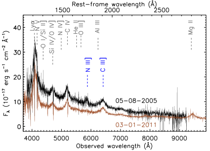
Figure 1: Optical (rest-frame ultraviolet) spectra of SDSS J1204+3518 (redshift $z=2.359$) reveal decreased N III] $\lambda$1750/C III] $\lambda$1909. The earlier-epoch (later-epoch) spectrum from SDSS (BOSS) is shown in black (brown).

2 Discovery of SDSS J1204+3518 as a Candidate TDE

2.1 N III] $\lambda$1750/C III] $\lambda$1909 Intensity Ratio Decay

Figure 1 shows the two archival spectra of SDSS J1204+3518. The SDSS spectrum was taken on 05-08-2005, whereas the BOSS spectrum was taken on 03-01-2011, i.e., 1.7 years (in the quasar’s rest frame) after the SDSS spectrum. The flux intensity of the N III] $\lambda$1750 emission decayed significantly, whereas C III] $\lambda$1909 stayed constant within uncertainties (see Figure 2 and Table 1 for details). We do not detect significant blueshift or redshift in N III] $\lambda$1750.

We do not detect significant N IV] $\lambda$1486 or He II $\lambda$1640 in either epoch (see §5.1 for discussion). The intensity of N V $\lambda$1240 seems to have decayed (Appendix A, Figure 8), though, it is highly uncertain due to the blending with Ly$\alpha$. We cannot robustly disentangle broad N V $\lambda$1240 absorption, if any, from emission due to blending and the intrinsically broad widths of the lines.

The narrow absorption lines seen in the spectra include four intervening C IV $\lambda\lambda$1548,1551 doublet systems and two associated systems (a C IV $\lambda\lambda$1548,1551 doublet and a N V $\lambda\lambda$1239,1243 doublet) that have consistent redshifts (Appendix A, Figure 9). There are no clear and significant variations in the strengths or velocities of the narrow absorption lines.

2.2 Origin of the Rapid Abundance Ratio Variability

The significant N/C decrease observed in SDSS J1204+3518 based on the N III] $\lambda$1750/C III] $\lambda$1909 emission-line intensity ratio cannot be easily explained by extreme metallicities. The timescales for the stellar population evolution necessary for metallicity changes (in quasar host galaxy stellar core or in the outer self-gravitating part of the accretion disk) are much longer than a few years.

Significant changes in the ionizing spectrum are unlikely given the similar ratios seen in the two-epoch spectra for other BLR emission lines such as the ionizing species of carbon (e.g., the C III] $\lambda$1909/C IV $\lambda$1549 intensity ratio is an indicator of the ionization level; Shields, 1976; Baldwin et al., 2003b, Table 1). Furthermore, the N III] $\lambda$1750/C III] $\lambda$1909 intensity ratio is sensitive to the N/C abundance ratio and is rather insensitive to the ionization parameter and the slope of the ionizing continuum (Shields, 1976; Osmer, 1980; Baldwin et al., 2003b; Yang et al., 2017).

Below we proceed with the hypothesis that the rapid N/C variability seen in SDSS J1204+3518 was caused by a candidate TDE of a star by the SMBH that powers the quasar.

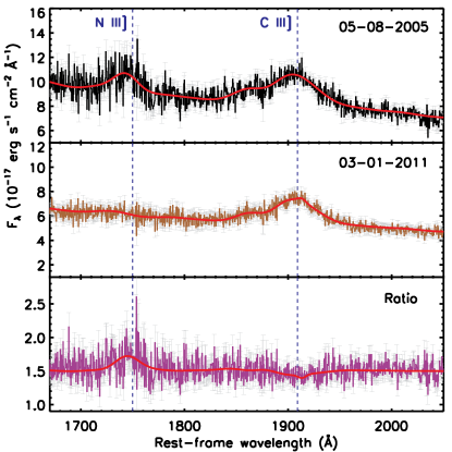
Figure 2: Spectral modeling of the N III] $\lambda$1750 and C III] $\lambda$1909 emission lines for SDSS J1204+3518. We show the flux density (thin black and brown curves), 1-$\sigma$ uncertainty (gray error bars), and our best-fit model (thick red curves) for the SDSS (top), BOSS (middle), and ratio (bottom) spectra.

Emission-line Measurements	SDSS	BOSS
N III] $\lambda$1750 Flux (10-16 erg s-1 cm-2) (1)	13.7$\pm$1.6	1.9$\pm$1.6
C III] $\lambda$1909 Flux (10-16 erg s-1 cm-2) (2)	32.6$\pm$4.4	31.2$\pm$4.2
C IV $\lambda$1549 Flux (10-16 erg s-1 cm-2) (3)	68.7$\pm$9.3	58.4$\pm$7.9
N III] $\lambda$1750/C III] $\lambda$1909  (4)	0.42$\pm$0.08	0.06$\pm$0.06
C III] $\lambda$1909/C IV $\lambda$1549  (5)	0.47$\pm$0.09	0.53$\pm$0.10
C IV $\lambda$1549 FWHM (km s-1) (6)	6810$\pm$400	6640$\pm$470
Mg II $\lambda$2800 FWHM (km s-1) (7)	N/A	6040$\pm$290
N III] $\lambda$1750 EW (Å) (8)	4.53$\pm$0.53	1.12$\pm$0.94
C III] $\lambda$1909 EW (Å) (9)	12.5$\pm$1.7	18.5$\pm$2.5
C IV $\lambda$1549 EW (Å) (10)	19.2$\pm$2.6	26.8$\pm$3.6

Table 1: Emission-line Measurements from the SDSS and BOSS Spectra. Note. Lines (1)–(3): emission-line flux intensity. The Si III] $\lambda$1892 and Al III $\lambda$1857 lines have been deblended and subtracted from the C III] $\lambda$1909 complex. Lines (4), (5): emission-line intensity ratio. Lines (6), (7): FWHM of the emission line. The SDSS spectrum does not cover Mg II $\lambda$2800. Lines (8)–(10): rest-frame equivalent width of the emission line. Errors quoted are 1-$\sigma$ uncertainties estimated from Monte Carlo simulations (for flux, FWHM, and EW measurements) or calculated from error propagation (for emission-line flux ratios).

2.3 Optical Light Curves

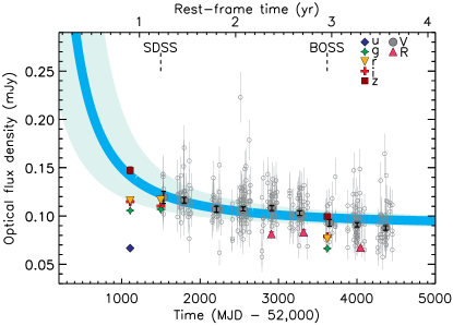
Figure 3: Optical light curves of the quasar SDSS J1204+3518. The data are from the CRTS (V band), PTF (R band), and SDSS ($u$, $g$, $r$, $i$, and $z$ band) surveys. We show both the individual (small open circles) and yearly inverse-variance-weighted mean (large filled circles) values for the CRTS data. We only show the yearly inverse-variance-weighted mean (large filled upward-facing triangles) for the PTF data to avoid overcrowding. The yearly inverse-variance-weighted mean values are centered on the median epoch of all the observations in a given year. Error bars denote the 1$\sigma$ uncertainty in the mean flux density of a given year. Also shown is the synthetic flux density in the corresponding SDSS filter calculated from the SDSS and BOSS spectra (the epoch of which is indicated by dashed lines). The cyan shading indicates the model of a $t^{-5/3}$ decay plus a constant background (with the light cyan shading representing 1$\sigma$ errors; see §§3.2 & 3.3 for details).

The optical (rest-frame UV) light curves of SDSS J1204+3518 are qualitatively consistent with the TDE hypothesis, though the baseline falls short of a proof. Figure 3 shows the heterogenous set of archival data spanning photometric epochs from 2002 to 2013, encompassing the two spectroscopic epochs. There is evidence of a decaying component in the flux on top of a background of stochastic variability (at the level of $\sim$10%) typically seen in optical quasars. As a toy model, we fit the light-curve data using the combination of a constant background plus a decaying component as $f\propto t^{\alpha}$ (see §§3.2 & 3.3 for details) where $\alpha=-5/3$ is expected for TDEs for stars according to conventional TDE theory (Rees, 1988). A fit to the V-band data assuming $\alpha=-5/3$ and a constant background of 0.09 mJy yields a peak-luminosity date of 51,860$\pm$240 (MJD), which is $\sim$1.3 years (rest-frame) before the “nitrogen-high” state caught in the SDSS spectrum. The fit is highly uncertain since the peak-luminosity date is unknown. A model with $\alpha=-4$ (expected for TDEs of partially disrupted stars; Guillochon & Ramirez-Ruiz, 2013) fits the data equally well.

Our toy models are for the purpose of illustration only and are not meant to be proof of a TDE. Recent observations have shown that the conventional $t^{-5/3}$ profile provides a poor fit to the light curves of most low-redshift TDEs (Arcavi et al., 2014; Holoien et al., 2014, 2016a, 2016b; Brown et al., 2016, 2017; Gezari et al., 2017). A range of power-law profiles seem to fit various decline rates at different times after disruption.

While the available optical light-curve data are broadly consistent with our baseline model, the null hypothesis (i.e., purely stochastic quasar variability) cannot be easily ruled out given the limited temporal coverage and the poor photometric accuracy for most of the light-curve data. Nevertheless, the large variability amplitude observed ($\gtrsim 30$%) is unusual for purely stochastic quasar variability given its estimated high Eddington rate (§3.5), since high Eddington-rate quasars are unlikely to show large variability (Rumbaugh et al., 2018). §5.2 discusses the brightness of the flare showing that it can be accommodated under the TDE hypothesis.

2.4 X-Ray Observations

Archival X-ray observations of SDSS J1204+3518 are broadly consistent with the TDE hypothesis. The X-ray flux decayed by $\sim$40% over rest-frame $\sim$0.3 years (within 1 rest-frame year after the assumed peak luminosity date; §3.6), in agreement with our toy model at least qualitatively. Furthermore, An archival XMM-Newton observation taken on MJD=52820 suggests an extremely soft X-ray spectrum (“photometric” X-ray photon index $\Gamma_{\rm X}=4.1$ estimated from the slope between the luminosities at 1 and 5 keV; Lusso & Risaliti, 2016)). This is similar to X-ray flares in low-redshift TDEs ($\Gamma_{\rm X}\gtrsim 4$; e.g., Bade et al., 1996; Komossa & Greiner, 1999; Lin et al., 2015; Auchettl et al., 2017, 2018), but is significantly different from typical optical quasars with $\Gamma_{\rm X}\approx 1.9$ (Young et al., 2009). We have analyzed the distribution of $\Gamma_{\rm X}$ using archival XMM-Newton observations for a control sample of ordinary quasars (Lusso & Risaliti, 2016) that have similar redshift and luminosity to SDSS J1204+3518. SDSS J1204+3518 is a $\sim$4$\sigma$ outlier in the distribution of $\Gamma_{\rm X}$. An archival Chandra observation taken on MJD=52476 also suggests a soft X-ray spectrum, though, the counts were too few for a robust measurement. §3.6 presents details on the X-ray data and analysis.

3 Details on the Data and Methods

3.1 Optical Spectroscopic Data and Analysis

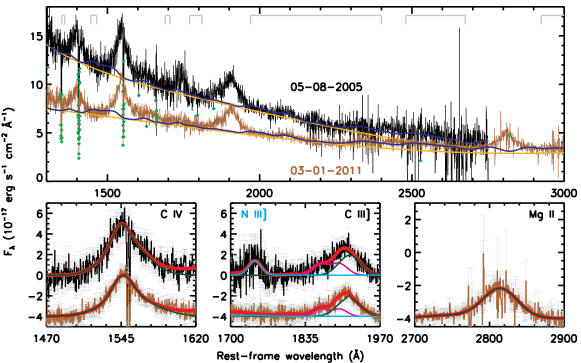
Figure 4: Spectral model fits for SDSS J1204+3518. The SDSS spectrum is shown in black and the BOSS spectrum is shown in brown. Top panel shows the global fit to the pseudo-continuum (with the combined pseudo-continuum model in blue and the power-law component in orange). The line segments in gray denote the wavelength windows adopted for the pseudo-continuum modeling. The diamonds in green mark the pixels that have been rejected in the fit (from either absorption lines or bad pixels). Bottom panels exhibit the model fits to the emission-line-only spectra (i.e., after subtracting the pseudo-continuum models) over the C IV $\lambda$1549, N III] $\lambda$1750–C III] $\lambda$1909, and Mg II $\lambda$2800 regions, respectively (with the combined emission-line model shown in red, the C IV $\lambda$1549, C III] $\lambda$1909, and Mg II $\lambda$2800 component in dark green, the Al III $\lambda$1857 and Si III] $\lambda$1892 complex in magenta, and the N III] $\lambda$1750 component in cyan). The error bars show the 1-$\sigma$ measurement error in the flux density. The BOSS emission-line-only spectrum is offset vertically by $-4\times 10^{-17}$ erg s^-1 cm^-2 Å^-1 for clarity.

SDSS J1204+3518 is contained in the SDSS DR7 quasar catalog (Schneider et al., 2010; Shen et al., 2011). It has two spectra available from the SDSS DR13 data archive. The first epoch spectrum (Plate = 2089, Fiber ID = 328, MJD = 53498) was from the SDSS-I/II survey (York et al., 2000) and the second epoch (Plate = 4610, Fiber ID = 652, MJD = 55621) was taken by the BOSS spectrograph within the SDSS-III survey (Dawson et al., 2013). The SDSS spectrum covers the wavelength range of 3800–9200 Å with a spectral resolution of $R=$1850–2200, whereas the BOSS spectrum covers 3650–10400 Å with a similar spectral resolution.

To measure the intensity ratio N III] $\lambda$1750/C III] $\lambda$1909 (“NCR” for short, defined in Equation 2) as an indicator of the N/C abundance ratio, we fit spectral models to the observed spectra following the procedures as described in detail in Shen & Liu (2012). The model is a linear combination of a power-law continuum, a pseudo-continuum constructed from Fe II emission templates, and single or multiple Gaussians for the emission lines. As the uncertainties in the continuum model may induce subtle effects on measurements of the weak emission lines, we first perform a global fit to the emission-line free region to better quantify the continuum components. After subtracting the continuum we then fit multiple Gaussian models to the emission lines around the N III] $\lambda$1750 and C III] $\lambda$1909 region locally. The C IV $\lambda$1549 region is also fit locally but separately to measure the intensity ratio C III] $\lambda$1909/C IV $\lambda$1549 (“CCR” for short, defined in Equation 3) as an indicator of the ionization parameter or the hardness of the ionizing continuum. We also fit the Mg II $\lambda$2800 region for virial black hole mass estimates from the BOSS spectrum.

More specifically, we model the N III] $\lambda$1750 line with a single Gaussian whose center and width are free parameters. We fit the wavelength range rest-frame 1700–1970 Å. We model the C III] $\lambda$1909 line using up to two Gaussians. We adopt two Gaussians for the Si III] $\lambda$1892 and Al III $\lambda$1857 lines which are often blended with the blue side of C III] $\lambda$1909. To break degeneracy in decomposing the C III] $\lambda$1909 complex, we tie the centers of the two Gaussians for C III] $\lambda$1909 (i.e., the C III] $\lambda$1909 emission-line profile is constrained to be symmetric); we also tie the velocity offsets of Si III] $\lambda$1892 and Al III $\lambda$1857 (relative to C III] $\lambda$1909) to the laboratory values. We also adopt three additional Gaussians for the other possibly detectable emission lines in the region (N IV] $\lambda$1718, Fe II UV 191 at 1786.7 Å, and Si II $\lambda$1816; Baldwin et al., 2003b). For the C IV $\lambda$1549 line, we fit the rest-frame wavelength range 1500–1700 Å. We model the C IV $\lambda$1549 line using two Gaussians. We adopt four additional Gaussians for the narrow and broad components of He II $\lambda$1640 and O III] $\lambda$1663. For the Mg II $\lambda$2800 line (covered only in the BOSS spectrum but not in the SDSS spectrum), we fit the wavelength range rest-frame 2700–2790 Å. We model the Mg II $\lambda$2800 line using a combination of up to two Gaussians for the broad component and one Gaussian for the narrow component. We impose an upper limit of 1200 km s^-1 for the FWHM of the narrow lines. As an example, Figure 4 shows our spectral decomposition modeling for SDSS J1204+3518. Figure 8 shows the spectral fit around the N V $\lambda$1240 region, which is highly uncertain because of blending. Figure 9 shows the narrow absorption line systems seen in the spectra of SDSS J1204+3518. Appendix B discusses further checks on systematic uncertainties of the spectra.

3.2 Optical Light-curve Data and Analysis

SDSS J1204+3518 has available light-curve data from the Catalina Real-time Transient Survey (CRTS; Drake et al., 2009, $V$ band), the Palomar Transient Factory (PTF; Law et al., 2009, $R$ band), and the SDSS ($u$, $g$, $r$, $i$, and $z$ bands). The SDSS measurements have the smallest photometric uncertainties, but there is only one photometric epoch and two subsequent spectroscopic epochs. We estimate the synthetic flux density in the corresponding SDSS filter calculated from convolving the SDSS and BOSS spectra with the filter throughput curves. We adopt the CRTS $V$-band magnitudes (converted to flux measurements) for fitting the light-curve model because they cover the longest time baseline that encompasses the two spectroscopic epochs. The PTF data do not provide more temporal coverage but serve as a double check for systematics. To mitigate the large photometric uncertainties associated with the CRTS and PTF data, we focus on the yearly inverse-variance-weighted-mean values in the analysis. We provide all the available photometry data in the literature in Table 2. We have also checked the available LINEAR (Sesar et al., 2011) data (re-calibrated to SDSS $r$ band) that extends the temporal coverage to earlier epochs, but SDSS J1204+3518 is close to the detection limit of the survey and its photometric uncertainties are too uncertain to be included in the analysis.

	$V$ (CRTS)	$R$ (PTF)	$u$ (SDSS)	$g$ (SDSS)	$r$ (SDSS)	$i$ (SDSS)	$z$ (SDSS)
MJD	(Vega mag)	(Vega mag)	(AB mag)	(AB mag)	(AB mag)	(AB mag)	(AB mag)
53,108	…	…	19.34 (0.03)	18.84 (0.01)	18.74 (0.01)	18.75 (0.01)	18.48 (0.03)
53,712.45	18.52 (0.14)	…	…	…	…	…	…
53,712.46	18.89 (0.16)	…	…	…	…	…	…
53,712.47	18.66 (0.15)	…	…	…	…	…	…
53,712.48	18.67 (0.15)	…	…	…	…	…	…
53,527.20	18.77 (0.15)	…	…	…	…	…	…
53,527.21	18.71 (0.15)	…	…	…	…	…	…
53,527.22	18.49 (0.14)	…	…	…	…	…	…
53,527.23	18.51 (0.14)	…	…	…	…	…	…
53,534.16	18.86 (0.16)	…	…	…	…	…	…
53,534.17	18.70 (0.15)	…	…	…	…	…	…

Table 2: Optical Photometry from the Literature. This table is available in its entirety in machine-readable form.

3.3 Fits to the Optical Light Curve

The $V$-band corresponds to the rest-frame UV that best traces the mass accretion rate in TDEs. We fit the light curve with $C+f(t)$ where $C$ is a constant and $f(t)$ is a power law of the form

$$f(t)=f_{0}\times(t+t_{0})^{\alpha}.$$ (1)

A fit to the nine data points assuming $\alpha=-5/3$ and a fixed constant background of $C=$0.09 mJy (estimated using the latest CRTS epochs) yields a best-fit model of $t_{0}=-51,860\pm$240 (MJD) and $f_{0}=7.5\pm 1.5$ Jy ($\chi^{2}/\nu=4.3$ for $\nu=$ seven degrees of freedom). Assuming $\alpha=-5/3$ and a positive constant background yields a model of $C=0.00$ mJy, $t_{0}=-39,500\pm$1500 (MJD), and $f_{0}=(1.0\pm 0.2)\times 10^{3}$ Jy ($\chi^{2}/\nu=1.4$ for $\nu=$ six degrees of freedom). While the latter model is statistically improved, we prefer the former model since the background quasar emission should be nonzero. The implied shorter evolutionary timescale is also more consistent with the variability timescale suggested by the two-epoch spectra. Allowing $\alpha$ to vary instead (assuming a fixed constant background of $C=$0.09 mJy) does not provide a statistically significant improvement to the fit (yielding $\chi^{2}/\nu=4.0$ for $\nu=$ six degrees of freedom for a model of $\alpha=-3.97\pm 0.05$).

3.4 Estimation of the Candidate TDE Luminosity and Energy

Assuming a constant background quasar emission of 0.09 mJy, we estimate that the $V$-band brightness of the candidate TDE is $\sim$0.04 mJy at MJD$\sim$53,000. At the redshift of $z=2.359$, the implied absolute $V$-band magnitude is $M_{V}=-23.4$ mag, assuming a Friedmann-Robertson-Walker cosmology with $\Omega_{m}=0.3$, $\Omega_{\Lambda}=0.7$, and $h=0.7$. A K-correction of 3.1 mag has been applied assuming that the unknown SED follows a black body with $T=2\times 10^{4}$ K which implies a rest-frame $V$-band apparent magnitude of $\sim$2.4 $\mu$Jy at MJD$\sim$53,000. Assuming that the $V$-band bolometric correction is in the range of 1.8–60 (appropriate for black body temperatures of $10^{4}$–5$\times 10^{4}$ K as observed in known TDEs; Tadhunter et al., 2017), the bolometric luminosity of the candidate TDE is estimated to be in the range of $9.5\times 10^{44}$—$3.2\times 10^{46}$ erg s^-1 at MJD$\sim$53,000. The total energy released during the observed part of the candidate TDE flare (using a simple trapezium rule integration of the $V$-band light curve) was estimated as $\sim 1\times 10^{52}$–$4\times 10^{53}$ erg. The implied total mass accreted by the black hole (from the candidate TDE only) is estimated as $\sim 0.02$–$0.5M_{\odot}$, assuming an accretion disk efficiency of $\eta=0.42$ for a Kerr black hole (Leloudas et al., 2016). This is a lower limit because the peak luminosity is not covered by the available light-curve data.

3.5 Estimation of the Black Hole Mass and Eddington Ratio

We estimate the black hole mass using the single-epoch estimator assuming virialized motion in the broad-line region clouds (Shen, 2013). Spectral fit to the SDSS spectrum suggests a C IV $\lambda$1549-based virial mass of $M_{\bullet}=10^{9.6\pm 0.1}M_{\odot}$ (statistical error only) using the calibrations of Vestergaard & Peterson (2006). The BOSS spectrum suggests a C IV $\lambda$1549-based virial mass of $M_{\bullet}=10^{9.5\pm 0.1}M_{\odot}$, or a Mg II $\lambda$2800-based virial mass estimate of $M_{\bullet}=10^{9.3\pm 0.1}M_{\odot}$, using the calibrations of Vestergaard & Osmer (2009) for Mg II $\lambda$2800. We adopt the BOSS estimates as our baseline values because they are more representative of the nitrogen-low (i.e., more steady accretion) state of the black hole. Mg II $\lambda$2800-based masses are generally considered more reliable than C IV $\lambda$1549-based masses (e.g., Shen, 2013), given the larger scatter between C IV $\lambda$1549 and H$\beta$ masses for high-redshift quasars (e.g., Shen & Liu, 2012). C IV $\lambda$1549 is more subject to nonvirial motion such as outflows. We estimate the Eddington ratio as $L_{{\rm bol}}/L_{{\rm Edd}}$, where the Eddington luminosity is $L_{{\rm Edd}}=M_{\bullet}/M_{\odot}\times 10^{38}$ erg s^-1 and the bolometric luminosity $L_{{\rm bol}}$ is calculated from $L_{{\rm 1350}}$ using the bolometric correction BC₁₃₅₀=3.81 from the composite quasar SED of Richards et al. (2006).

3.6 X-Ray Data and Analysis

There are three X-ray observations of the field of SDSS J1204+3518 available in the public data archives. The ROSAT All Sky Survey (RASS; Voges et al., 1999, 2000) scan with the Position Sensitive Proportional Counter (Pfeffermann et al., 1987) from 1990 November yielded a 3$\sigma$ upper limit of 0.02 counts s^-1, corresponding to an unabsorbed X-ray flux limit of $F_{{\rm 0.1-2.4\,keV}}<2.9\times 10^{-13}$ erg cm^-2 s^-1 (assuming a $\Gamma_{{\rm X}}=2$ power-law spectrum corrected for the Galactic column density of $1.7\times 10^{20}$ cm^-2; Dickey & Lockman, 1990).

A Chandra observation of HS 1202$+$3538 (observation ID=3070) on 2002 July 21 (MJD=52476) serendipitously caught SDSS J1204+3518 at an off-axis angle of 10.7 arcmin. The observed-frame soft (0.5–2 keV) and hard (2–8 keV) counts in the 6.7 ks (4.5 ks corrected for vignetting) exposure were 16 and 9, respectively (Gibson et al., 2008). We derive an unabsorbed X-ray flux (corrected for the Galactic column density) of $F_{{\rm 0.5-10\,keV}}=2.6\times 10^{-14}$ erg cm^-2 s^-1 for $\Gamma_{{\rm X}}=4$, or $F_{{\rm 0.5-10\,keV}}=4.4\times 10^{-14}$ erg cm^-2 s^-1 for $\Gamma_{{\rm X}}=2$. The X-ray counts are too few for a robust measurement of $\Gamma_{\rm X}$. Nevertheless, the hardness ratio HR $\equiv({\rm H}-{\rm S})/({\rm H}+{\rm S})=-0.28$ suggests a soft X-ray spectrum, similar to the values observed in the X-ray flares of TDEs not long after peak luminosity (Auchettl et al., 2017).

Finally, SDSS J1204+3518 is contained in the 3XMM serendipitous source catalog DR5 (Rosen et al., 2016) with DETID=101487424010032. The XMM-Newton European Photon Imaging Camera detected SDSS J1204+3518 on 2003 May 23 and 2003 June 30. The longer exposure taken on 2003 June 30 (observation ID=0148742401) covered SDSS J1204+3518 with a “live” exposure time of 20.1 ks at an off-axis angle of 10.0 arcmin. The X-ray photon index estimated from the slope between the luminosities at 1 and 5 keV is 4.09 with an X-ray S/N = 4.7 (Lusso & Risaliti, 2016). This “photometric” X-ray photon index is not as reliable as the spectroscopic tracer, but provides a reasonable estimate of the X-ray spectral hardness. The derived unabsorbed X-ray flux (averaged over the two XMM-Newton epochs) is $F_{{\rm 0.5-10\,keV}}=1.5\times 10^{-14}$ erg cm^-2 s^-1 for $\Gamma_{{\rm X}}=4$, or $F_{{\rm 0.5-10\,keV}}=1.9\times 10^{-14}$ erg cm^-2 s^-1 for $\Gamma_{{\rm X}}=2$. For the Chandra and XMM-Newton detections, we adopt the X-ray estimates from assuming $\Gamma_{{\rm X}}=4$ as our baseline values (shown in Figure 3), although the qualitative decaying trend still holds for $\Gamma_{{\rm X}}=2$.

3.7 Radio Loudness Upper Limit from FIRST

SDSS J1204+3518 was covered by the FIRST survey footprint but was undetected with a 3$\sigma$ upper limit of $f^{{\rm obs}}_{{\rm 6\,cm}}<$ 0.381 mJy. Assuming that the radio flux follows a power law (i.e., $f_{\nu}\propto\nu^{\alpha}$), this translates into $f^{{\rm rest}}_{{\rm 6\,cm}}<$0.70 mJy for a spectral index $\alpha=-0.5$ (Jiang et al., 2007), or $<$1.0 mJy assuming $\alpha=-0.8$ (Gibson et al., 2008). Combined with the $f_{{\rm 2500}}$ measurement from the optical spectrum, the implied limit on the radio loudness parameter (Kellermann et al., 1989), i.e., $R\equiv f_{{\rm 6\,cm}}/f_{{\rm 2500}}$, is $<$4.9 ($<$7.8) using the SDSS (BOSS) spectrum assuming $\alpha=-0.5$, or $<$7.2 ($<$11) assuming $\alpha=-0.8$, which is marginally inconsistent with the radio-loud criterion R$>$10.

4 Statistical Context for the Single-object Discovery

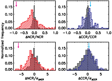
Figure 5: Probability distribution of intensity ratio variability reveals statistical evidence for N III] $\lambda$1750/C III] $\lambda$1909 (“NCR” for short) decreasing over $>$1 year timescales in N-rich quasars, whereas C III] $\lambda$1909/C IV $\lambda$1549 (“CCR” for short) remains unchanged. Negative values denote decreasing with time. The dashed histograms show the long-term (rest-frame $\Delta t>1$ year) variability. The gray histograms represent the short-term (rest-frame $\Delta t<1$ month) variability that is consistent with being purely due to statistical noise. The upper panels show the fractional (or relative) variability of the emission-line intensity ratio whereas the lower panels display the S/N of the variability (i.e., variability normalized by measurement uncertainty accounting for both statistical and systematic errors). Arrows indicate the measurements for SDSS J1204+3518. See §4.2 for details.

4.1 Sample Selection

We start with a sample of 311 N-rich quasars by combining two N-rich quasar catalogs in the literature (Jiang et al., 2008; Batra & Baldwin, 2014). The first catalog (Jiang et al., 2008) contains 293 quasars at $1.7<z<4.0$ with strong N IV] $\lambda$1486 or N III] $\lambda$1750 emission lines (rest-frame EW$>3$ Å). The second catalog contains 43 quasars (of which 25 overlap with the first catalog) at $2.29<z<3.61$ that have the strongest N IV] $\lambda$1486 and N III] $\lambda$1750 lines in addition to strong N V $\lambda$1240 lines. Both catalogs were selected from the fourth edition of the SDSS Quasar Catalog (Schneider et al., 2007) based on the SDSS fifth data release (Adelman-McCarthy et al., 2007).

To study spectroscopic variability for these N-rich quasars, we analyze all the available high-quality spectrum pairs (with median S/N $>$10 pixel^-1 over rest-frame 1700–2000 Å) in the SDSS thirteenth data release (SDSS Collaboration et al., 2016) for a sample of 82 unique quasars. We visually examine the ratio spectrum (similar to that shown in the lower panel of Figure 2 but over the entire relevant spectral range) for each spectrum pair; SDSS J1204+3518 was identified as our best candidate for having significant N/C variability (i.e., the ratio spectrum changed significantly over the N III] $\lambda$1750 region but stayed constant over the C III] $\lambda$1909 region). There are 193 high-quality spectrum pairs with rest-frame time separations $>$1 year (for 78 of the 82 unique N-rich quasars; the other 4 only have high S/N repeat spectra separated by $<$ 1 year). This “long-term” group serves as our parent sample for estimating the fraction of N-rich quasars that show significant N/C variability over $\gtrsim$ 1year timescales. To calibrate measurement uncertainties, we also define a control sample of a “short-term” group containing 355 high-quality spectrum pairs for N-rich quasars with rest-frame time separations $<$1 month. The median time baseline $<\Delta t>$ in the “long-term” (“short-term”) group is 2.7 (0.034) years (rest frame).

4.2 Statistical Analysis

Sample	Short-term ($<$1 mon)			Long-term ($>$1 years)
Measurements	($<\Delta t>$ = 0.4 mon)			($<\Delta t>$ = 2.7 years)
Statistics	Median	SD		Median	SD	Pnull
$\Delta$NCR/NCR	$-$0.01$\pm$0.01	0.14		$-$0.12$\pm$0.08	1.2	10-21
$\Delta$CCR/CCR	0.00$\pm$0.01	0.18		0.06$\pm$0.06	0.79	10-8
$\Delta$NCR/$\sigma_{\Delta{\rm NCR}}$	$-$0.2$\pm$0.1	1.4		$-$1.0$\pm$0.2	2.8	10-10
$\Delta$CCR/$\sigma_{\Delta{\rm CCR}}$	0.0$\pm$0.2	3.1		0.5$\pm$0.2	2.2	0.05

Table 3: Emission-line Intensity Ratio Variability Statistics. Note. NCR stands for the N III] $\lambda$1750/C III] $\lambda$1909 intensity ratio and CCR stands for the C III] $\lambda$1909/C IV $\lambda$1549 intensity ratio. The difference is defined as the later epoch minus the earlier epoch so that negative values mean a decrease in the intensity ratios over time. The long-term (short-term) sample contains 193 (355) pairs of high-quality spectra for N-rich quasars. SD: standard deviation. P_null: null probability from the Kolmogorov–Smirnov test of the long-term ($>$1 years) sample compared against the short-term ($<$1 month) sample. See §4.2 for details.

Figure 5 (upper left panel) shows the distribution of the fractional variability in the N III] $\lambda$1750/C III] $\lambda$1909 emission-line intensity ratio (“NCR” for short). We define the fractional variability as

$$\Delta{\rm NCR/NCR}\equiv({\rm N/C}_{2}-{\rm N/C}_{1})/({\rm N/C}_{1}),$$ (2)

where N/C₁ is from the earlier epoch and N/C₂ is from the later epoch. Negative values mean a decrease in N/C over time. Monte Carlo simulations suggest that the observed distribution of the short-term NCR variability is consistent with being purely induced by statistical noise. The dispersion in $\Delta$NCR/NCR for the long-term pairs is significantly larger than that in the short-term pairs (with the standard deviation (SD) being 1.2 for the long-term sample compared to 0.14 for the short-term sample; Table 3). This much larger scatter is most likely caused by systematic uncertainties associated with continuum modeling, which is larger in the long-term pairs due to increased quasar variability (e.g., MacLeod et al., 2010; Morganson et al., 2014).

Figure 5 also shows the effective “S/N” of the NCR and CCR variation (lower panels), i.e., emission-line intensity ratio variation normalized by measurement uncertainties (accounting for both statistical and systematic errors). The dispersion in $\Delta$NCR/$\sigma_{\Delta{\rm NCR}}$ for the long-term pairs is more similar to that in the short-term pairs after the normalization (with SD being 2.8 for the long-term sample compared to 1.4 for the short-term sample), that accounts for differences in the systematic uncertainties. The long-term sample shows a 5$\sigma$ detection that the median value is nonzero ($-1.0\pm 0.2$, where 0.2 is the 1-$\sigma$ error in the median, estimated as SD$/\sqrt{N}$, where $N$ is the number of data points; Table 3). Furthermore, its probability distribution is significantly different from that expected from pure measurement noise as characterized by the short-term pairs. Kolmogorov–Smirnov test shows that the probability that the two distributions are drawn from the same sample $P_{{\rm null}}$ is $10^{-10}$ (Table 3). Compared to the control sample of short-term pairs, the long-term pairs show a net negative $\Delta$NCR/$\sigma_{\Delta{\rm NCR}}$, providing statistical evidence that NCR decreases with time in N-rich quasars. SDSS J1204+3518 stands out among those that show the most significant decreases in the NCR. We have checked the other positive and negative value tails seen in the $\Delta$NCR/NCR distribution, which are largely caused by systematic uncertainties from our emission-line measurements and do not show significant variability in the flux-ratio spectrum.

Figure 5 (upper right panel) also shows that the C III] $\lambda$1909/C IV $\lambda$1549 emission-line intensity ratio (“CCR” for short) variation. Similarly to the NCR variation, it is defined as

$$\Delta{\rm CCR/CCR}\equiv({\rm C3/C4}_{2}-{\rm C3/C4}_{1})/({\rm C3/C4}_{1}),$$ (3)

where C3/C4₁ is from the earlier epoch and C3/C4₂ is from the later epoch. The long-term CCR variation, on the other hand, is more similar to the short-term CCR variation. While the dispersion is still larger for the long-term CCR variation in terms of $\Delta$CCR/CCR (SD being 0.79 for the long-term compared to 0.18 for the short-term sample; Table 3), their difference is smaller than that in the dispersion of $\Delta$NCR/NCR (a factor of $\sim 4$ difference rather than $\sim 9$). This is understandable considering that stronger lines (i.e., C IV $\lambda$1549) are less affected by systematic uncertainties in the continuum modeling. In terms of $\Delta$CCR/$\sigma_{\Delta{\rm CCR}}$, i.e., after normalizing the measurement uncertainties, the median value of the long-term sample is consistent with being zero within 2.5 $\sigma$ ($0.5\pm 0.2$; Table 3); the 2.5$\sigma$ positive deviation from zero is most likely explained by a noise-induced bias, as we discuss below. Furthermore, the long-term and short-term distributions are statistically identical (with $P_{{\rm null}}$ being 0.05; Table 3). SDSS J1204+3518 does not show significant CCR variation. Table 3 summarizes the statistical properties of the NCR and CCR variability measurements.

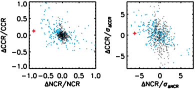
Figure 6: Test on NCR versus CCR. While CCR appears to be increasing as NCR decreases in the long-term sample (shown with cyan dots), this apparent trend is also seen in the short-term sample (shown with black crosses), which is most likely caused by the inter-correlation between the NCR and CCR terms given measurement errors. The two parameters NCR and CCR are not independent from each other since the C III] $\lambda$1909 emission-line intensity is included in both terms. Considering measurement errors, a larger C III] (caused by noise) will result in a smaller NCR and a larger CCR. SDSS J1204+3518 is shown with a red star in both panels.

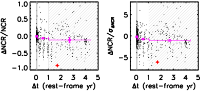
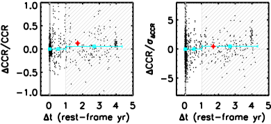
Figure 7: Examining the time dependence of intensity ratio variability. Negative values denote decreasing with time. Individual data points are shown with small black dots whereas large open squares denote median values in a given bin of time separation. Error bars denote uncertainties in the medians. The gray shaded region denotes the short-term (rest-frame $\Delta t<1$ month) sample, whereas the hatched region encloses the long-term (rest-frame $\Delta t>1$ years) sample. The left column shows the fractional (or relative) variability of the emission-line intensity ratio whereas the right column displays the S/N of the variability (i.e., variability normalized by measurement uncertainty). Stars indicate the measurements for SDSS J1204+3518.

Figure 6 examines whether there is any general trend between $\Delta$NCR/NCR and $\Delta$CCR/CCR. Although $\Delta$CCR/CCR appears to be increasing as $\Delta$NCR/NCR decreases in the long-term sample (shown with cyan dots), this apparent trend is also seen in the short-term sample (shown with black crosses), which is most likely caused by the correlation between the NCR and CCR terms due to measurement errors. The apparent trend arises because NCR and CCR are not independent from each other since the C III] $\lambda$1909 emission-line flux intensity is included in both terms. Considering measurement errors, a stronger C III] $\lambda$1909 (caused by noise) will lead to a smaller NCR and a larger CCR, resulting in an apparent anti-correlation between the NCR and CCR. This also likely explains the 2.5$\sigma$ positive deviation from zero in the median value of $\Delta$CCR/$\sigma_{\Delta{\rm CCR}}$ for the long-term sample, in which systematic uncertainty from continuum modeling adds to the error, resulting in more bias in the long-term sample than in the short-term sample because of increased quasar variability.

Figure 7 examines the potential time dependence of the intensity ratio variability. We show both the individual data points (small dots) and the median values in a given bin of time separation (large open squares with error bars denoting uncertainties in the median values) to help assess the general trend. While there is some hint of the variability increasing as a function of time in support of the TDE hypothesis, we cannot draw a firm conclusion in view of the limited dynamic range in time separation and the large scatter in the intensity ratio variability measurements.

5 Discussion and Future Work

5.1 Puzzles in the Emission Lines

The absence of evidence for strong variability in the N IV] $\lambda$1486 and He II $\lambda$1640 lines is puzzling, but does not rule out the TDE hypothesis. In the only three known TDEs with available UV spectra (Cenko et al., 2016; Yang et al., 2017; Brown et al., 2018), N IV] $\lambda$1486 (He II $\lambda$1640) is not always detected or relatively weak in some epochs, whereas N III] $\lambda$1750 is always detected. So empirically it is possible to see N III] $\lambda$1750 but not N IV] $\lambda$1486 (He II $\lambda$1640) emission in TDEs, which may be related to the different ionizing potentials of the lines. In addition, a practical complication is that N IV] $\lambda$1486 is on the extended blue wing of C IV $\lambda$1549 for SDSS J1204+3518 and may be buried underneath, especially if it is weak. For He II $\lambda$1640, another possibility is that if the disrupted star were about to ascend the giant branch, most helium would be sequestered in the dense helium core, which would not be disrupted by the more massive black hole (unlike in low-redshift TDEs around smaller black holes). Finally, our selection is based on the N III] $\lambda$1750/C III] $\lambda$1909 ratio variability so that we may have missed systems that show stronger N IV] $\lambda$1486 and/or He II $\lambda$1640 variability.

While bearing some resemblances to N-rich quasar spectra, none of the three TDEs with UV spectra exhibit C III] $\lambda$1909 or Mg II $\lambda$2800 emission features. Their C IV $\lambda$1549 is also much weaker than expected. The origins of these discrepancies are still open to debate. They might be due to differences in the physical conditions in the gas and on the shape of the ionizing continuum. For example, the absence of Mg II $\lambda$2800 could result from photoionization by the extremely hot continuum, which may be transient in nature as the continuum temperature eventually cools down (Cenko et al., 2016). The absence of C III] $\lambda$1909 could be due to collisional deexcitation if the gas density is above critical, $n=10^{9.5}$ cm^-3 (Osterbrock, 1989).

5.2 SDSS J1204+3518 Was Not Too Bright for a TDE

The brightness of the candidate TDE of $\sim$0.04 mJy at MJD$\sim$53,000 implies an absolute $V$-band magnitude of $-23.4$ mag at the redshift of the quasar. This is only $\sim 0.6$ mag fainter than the peak luminosity of ASASSN-15lh (Leloudas et al., 2016), the brightest TDE candidate reported to date (see Dong et al. 2016; Godoy-Rivera et al. 2017, however, for an alternative explanation for the nature of the source as a supernova). This high apparent brightness seems difficult to explain under the TDE hypothesis, but it is perhaps understandable for the following reasons. First, the observed $V$-band samples the rest-frame UV that is close to the peak of the spectral energy distribution (SED) of the candidate TDE, resulting in a large K-correction at the redshift of the quasar. This is dramatically different from local TDEs, in which the $V$ band only samples the Rayleigh-Jeans tail of the SED.

Second, the high luminosity of the candidate TDE could be explained by the large BH mass of the quasar and its likely rapid spin (see §§3.5 & 5.3 for details). In addition, TDEs in AGN hosts may have higher radiative efficiencies than those in inactive galactic nuclei potentially due to interaction of the stellar debris with the preexisting accretion disk (Blanchard et al., 2017). However, the estimated efficiency does not strain the Eddington limit even at the projected peak-luminosity date, which is highly uncertain. The total energy released would require the accretion of a mass of $\gtrsim$0.02–0.5$M_{\odot}$ (see §3.4 for details).

Finally, our sample is most likely highly biased to the most luminous events because: (i) by selection we are sensitive only to the high-redshift (i.e., $z>1.7$ for the relevant UV lines to be covered in the observed optical spectra) population, and (ii) the SDSS is not a particularly deep survey.

5.3 SMBH Mass and Spin of SDSS J1204+3518

Analysis of the BOSS spectrum suggests that the quasar is powered by an SMBH with a virial mass estimate of

$${\rm log}~{}(M_{\bullet}/M_{\odot})=9.3\pm 0.1\pm 0.5~{}{\rm dex,}$$ (4)

where 0.1 (0.5) dex is the 1$\sigma$ statistical (systematic) error (Shen, 2013). The implied Eddington ratio is $\sim$0.005–0.16 (for the candidate TDE flare component only, depending on the unknown SED; it is $\sim 0.13$ for the background quasar emission; see §3.5 for details) around MJD of 53,000 (i.e., $\sim 1$ rest-frame years post the peak-luminosity date), consistent with an initial sub-Eddington phase predicted by conventional TDE theory for massive BHs (Rees, 1988). Assuming a time lag of

$$t_{f}\sim 1.1(M_{\bullet}/10^{8}M_{\odot})^{1/2}r_{\star}^{3/2}m_{\star}^{-1}~{}{\rm years,}$$ (5)

where $r_{\star}\equiv R_{\star}/R_{\odot}$ and $m_{\star}\equiv M_{\star}/M_{\odot}$, between disruption and infall of the tightest-bound debris for a solar-type star, a black hole mass of $M_{\bullet}=10^{9.3}M_{\odot}$ would yield a Newtonian estimate of the disruption date of $\sim 46,000$ (MJD), i.e., $\sim 5$ rest-frame years before the peak-luminosity date. A relativistic estimate of the disruption date would be $\sim 50,000$ (MJD), i.e., $\sim 2$ rest-frame yr before the peak-luminosity date (Leloudas et al., 2016).

The gravitational radius increases with black hole mass at a higher rate than the tidal radius $R_{{\rm T}}$ does (i.e., $R_{g}\propto M_{\bullet}$ whereas $R_{{\rm T}}\propto M_{\bullet}^{1/3}$). Therefore, stars can be tidally disrupted before being swallowed whole into the horizon only if the black hole is less massive than the Hills mass $M_{{\rm Hills}}$, where

$$M_{{\rm Hills}}\approx 10^{8}M_{\odot}r_{\star}^{3/2}m_{\star}^{-1/2}$$ (6)

for non-spinning Schwarzschild black holes (Hills, 1975). $M_{{\rm Hills}}$ can be up to an order of magnitude larger for stars on optimal orbits around rapidly spinning Kerr black holes (Leloudas et al., 2016). The virial mass estimate of SDSS J1204+3518 suggests that a spinning Kerr black hole is required for all allowed masses. A main-sequence supersolar mass star on prograde equatorial orbits can be disrupted by a maximally spinning Kerr black hole with $M_{\bullet}=10^{8.9}M_{\odot}$, or a moderately spinning Kerr black hole with $M_{\bullet}=10^{8.5}M_{\odot}$. If the BH mass is in the higher end in the estimated range, then a giant star is required.

The rapid N/C variability, on the other hand, implies that the evolutionary timescale is not much longer than a few years. Assuming that it is driven by the circularization luminosity (but see, e.g., Jiang et al., 2016, for an alternative explanation) that evolves on the fallback timescale $t_{f}$, which is comparable to the viscous timescale in the accretion disk for massive black holes, the rapid evolution suggests that the disrupted is a main-sequence star rather than a giant. Future near-infrared spectroscopy of the Balmer lines and/or reverberation mapping observations are needed to help better constrain the black hole mass for SDSS J1204+3518.

5.4 SMBH Mass and Spin of N-rich versus Normal Quasars

A significant difference between N-rich and normal optical quasars is that N-rich quasars have systematically narrower widths of C IV $\lambda$1549 (Jiang et al., 2008; Batra & Baldwin, 2014). This implies, under standard assumptions, that N-rich quasars have less massive black holes than the normal quasar population. This is at odds with the more massive host galaxies implied by the high metallicity hypothesis given the galaxy mass-metallicity relation (Tremonti et al., 2004; Erb et al., 2006; Maiolino et al., 2008) and the SMBH-host mass correlation (Ferrarese & Merritt, 2000; Gebhardt et al., 2000; Tremaine et al., 2002; Kormendy & Ho, 2013; Graham, 2016). In contrast, the TDE scenario would provide a natural explanation for the narrower widths of C IV $\lambda$1549 seen in N-rich quasars since less massive black holes are more likely to disrupt stars.

N-rich quasars also have a significantly higher radio-loud fraction compared to normal optical quasars (Jiang et al., 2008). The origin of this difference is unknown. If the radio loudness is physically related to the black hole spin (Blandford & Znajek, 1977; Sikora et al., 2007), the TDE hypothesis may also explain the high radio-loud fraction in N-rich quasars, since black holes with larger spins are more prone to disrupting stars. SDSS J1204+3518 was undetected by the FIRST 1.4 GHz survey (White et al., 1997) whose upper limit was marginally inconsistent with being radio loud (see §3.7 for details).

5.5 Disrupting Giants versus Main-sequence Stars

SDSS J1204+3518 represents the first case of a quasar with significant N/C variability over yearly timescales. Our analysis on a large sample of N-rich quasars shows statistical evidence that N/C decays over time, while the ionization level remains unchanged (§4). However, similar to the case of Q0353$-$383 (Osmer, 1980; Baldwin et al., 2003b), the typical decay rate estimated in the average SDSS N-rich quasars (median $\Delta$NCR/NCR$=-12\pm$8% in $\sim$2.7 rest-frame years, or $\sim-4\pm$3% yr^-1; Table 3) is much less than that seen in SDSS J1204+3518 ($\Delta$NCR/NCR$=-86\pm$14% in 1.7 rest-frame years, or approximately $-50\pm$8% yr^-1; Table 1). This could be explained in the TDE scenario if most N-rich quasars were caused by TDEs of giants rather than main-sequence stars, since TDEs of giants would evolve more slowly (MacLeod et al., 2012). We cannot rule out the possibility that only some but not all of the N-rich quasars are caused by TDEs. Testing whether most N-rich quasars are due to TDEs of giants would require high S/N spectroscopic follow-up observations on much longer timescales (i.e., decades and even centuries) rather than being probed by current surveys.

While the lifetimes of giant stars are much shorter than those of main-sequence stars (and therefore TDEs of giants should be much less frequent), it is still possible for the N-rich population to be dominated by TDEs of giants considering the disruption constraint given the large black hole masses of high-redshift quasars (i.e., main-sequence stars are more likely to be swallowed whole rather than being disrupted unless the black hole mass is small enough and/or the spin is high), in contrast to the demographics seen in local, inactive galaxies with smaller black holes.

5.6 Implications on the TDE Rate in Quasar Hosts

We estimate the implied TDE rate in quasars assuming that (i) SDSS J1204+3518 is a TDE of a main-sequence star, and (ii) nearly all of the rest of N-rich quasars are TDEs of giants. The total order-of-magnitude rate is estimated as

$$r=r_{{\rm MS}}+r_{{\rm G}}=f_{{\rm N-rich}}\times\bigg{(}\frac{f_{{\rm MS}}}{{\rm 2~{}yr}}+\frac{f_{{\rm G}}}{{\rm 10^{3}~{}yr}}\bigg{)}\sim 10^{-4}~{}{\rm yr}^{-1}~{}{\rm galaxy}^{-1},$$ (7)

where $f_{{\rm N-rich}}\lesssim 10^{-2}$, $f_{{\rm MS}}\sim\frac{1}{78}$, and $0<f_{{\rm G}}\lesssim\frac{77}{78}$ ($f_{{\rm G}}\sim\frac{77}{78}$ assuming all N-rich quasars are TDEs). The evolution timescale (which goes into the denominator of the rate estimate) is much longer for TDEs of giants (MacLeod et al., 2012, here assumed to be $\sim 10^{3}$ years; assuming it is $\sim 10^{2}$ years instead would make $r_{{\rm G}}$ comparable to $r_{{\rm MS}}$ but still not an order-of-magnitude larger) so that their contribution to the estimated rate is small (or similar if $f_{{\rm G}}$ is close to unity) compared to that by SDSS J1204+3518 alone.

Under the TDE scenario, our systematic search implies a much higher TDE rate in quasars than in normal galaxies. The fraction of N-rich quasars is $\lesssim 1\%$, and we found one definitive case SDSS J1204+3518 out of a parent sample of 78 N-rich quasars in total within a time window of $\sim 2$ years (rest-frame). Thus the implied TDE rate is $\sim 10^{-4}$ yr^-1 galaxy^-1. This is $\sim$100 times higher than the expected TDE rate at $M_{\bullet}\sim 10^{9}M_{\odot}$, which is $\sim 10^{-6}$ yr^-1 galaxy^-1 for supersolar mass stars (Kochanek, 2016b). Similarly, the observed TDE rate in post-starburst galaxies is $\sim 100$ times higher than normal galaxies (Arcavi et al., 2014). This is perhaps not a coincidence since both quasars and post-starburst activities may be associated with recent merger events that would greatly increase the number of stars in low angular momentum orbits, fueling TDEs.

5.7 Future Directions

Our findings provide motivation for future research programs on N-rich quasars, which have been enigmatic and hard-to-understand objects until now. Despite their rarity, we show that N-rich quasars may be important links for understanding how SMBHs disrupt stars.

Examples of future research programs include:

1. Finding additional cases of TDEs of stars in quasars to establish their frequency of incidence and learn more about their astrophysics.

2. Learning more about the physics of the encounters of stars with SMBHs.

3. Provide improved knowledge of the evolutionary nature and distributions of stars near SMBHs. For example, time scales for disruption of giant stars are longer than for main-sequence stars.

The abundance ratio variability offers a potentially new method for identifying TDEs, complementary to the traditional method based on X-ray and/or UV/optical flux variability. In particular, it may open a new window of discovering TDEs at significantly higher redshifts ($z>2$) than previous work. In comparison, the majority of known TDEs are at low redshifts ($z<0.3$), and the current redshift record holder is Swift J2058+05 at $z=1.1853$ (Cenko et al., 2012). This has implications for the current efforts to use TDEs to study supermassive black holes. Its potential may be better realized with the upcoming large-scale time-domain spectroscopic surveys such as the SDSS-V (Kollmeier et al., 2017) and MSE (McConnachie et al., 2016) projects.

Appendix A Spectral Modeling for N V $\lambda$1240 and Narrow Absorption Line Systems

Figure 8 shows our spectral modeling for SDSS J1204+3518 around the N V $\lambda$1240 region. Figure 9 shows narrow absorption line systems seen in the spectra of SDSS J1204+3518.

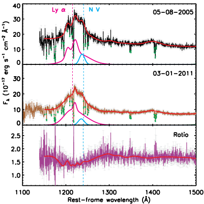
Figure 8: Spectral modeling for SDSS J1204+3518 around the N V $\lambda$1240 region. Shown are the flux density (thin black and brown curves), 1$\sigma$ uncertainty (gray error bars), and our best-fit model (thick red curves) for the SDSS (top), BOSS (middle), and ratio (bottom) spectrum. In the top and middle panels, we also plot models for the Ly$\alpha$ (magenta) and N V $\lambda$1240 (cyan) complex. Although N V $\lambda$1240 seems to have decayed at face value, it is highly uncertain due to blending with Ly$\alpha$ and possible contamination from broad absorption. Our model does not attempt to decouple emission from possible broad absorption because it is ambiguous given the broad widths of the lines. The diamonds in green mark the pixels from narrow absorption lines that have been rejected in the fit.

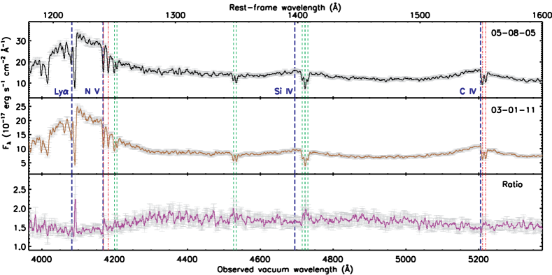
Figure 9: Narrow absorption line systems seen in the spectra of SDSS J1204+3518. Top (middle) panel shows the earlier-epoch (later-epoch) spectrum from SDSS (BOSS). Bottom panel shows the ratio spectrum. Blue thick long dashed lines mark the expected central wavelengths of the emission lines at the redshift of SDSS J1204+3518. Red thin dotted–dashed lines indicate narrow associated absorbers (a C IV $\lambda\lambda$1548,1551 doublet and a N V $\lambda\lambda$1239,1243 doublet) redshifted by $\sim 550$ km s^-1 to the quasar systemic redshift. Green thin dashed lines denote four intervening narrow C IV $\lambda\lambda$1548,1551 doublet absorbers (at the redshifts of 2.0506, 2.0455, 1.9238, and 1.7123) caused by the intergalactic medium along our line of sight to the quasar. All spectra have been smoothed by a 4-pixel boxcar for display purposes. Error bars indicate 1$\sigma$ uncertainties pixel^-1 before smoothing.

Appendix B Systematic Uncertainties

We use a Monte Carlo approach (Shen & Liu, 2012) to estimate measurement uncertainties, taking into account both statistical uncertainties due to flux errors and systematic uncertainties due to ambiguities in decomposing multiple model components. As we discuss below, we have carried out extensive tests to validate the significance of the N III] $\lambda$1750 emission in the SDSS spectrum. The detection is significant at the $>5\sigma$ confidence level and is unlikely to be explained by noise (counting both systematic and statistical uncertainties).

First, the SDSS and BOSS spectra were both co-added, combining six consecutive individual 15-minute exposures. We have checked the individual exposures (Figure 10) to verify our emission-line measurement based on the co-added spectra. Second, the N III] $\lambda$1750 feature is close to the dichroic edge of the SDSS spectrograph. To quantify possible systematic effects due to the dichroic edge, we have co-added and examined the individual SDSS spectra for the blue and red sides, separately. We have used the inverse-variance weighted mean to properly co-add the individual spectra. We have properly accounted for and rejected bad pixels.

Figure 10 (left panel) shows the co-added and individual blue SDSS spectrum. N III] $\lambda$1750 is detected in both the blue co-add and each and every of the individual exposures, although it is much more noisy in the individual spectra (so are the other emission lines). In particular, it is most clearly detected in the exposure with the highest S/N (shown in purple; the individual exposure spectrum is ordered with increasing median S/N over the 5700–6100 Å from top to bottom). We focus on the blue side here because it extends to the observed wavelengths of $\sim$6150 Å, which covers the entire N III] $\lambda$1750 feature. The red side only partially covers the N III] $\lambda$1750 feature. The fact that N III] $\lambda$1750 is detected in the blue-only spectrum argues against its origin as artifacts due to stitching together the red and blue spectra. Our final quoted detection significance is based on the co-added, blue–red stitched spectrum, because co-adding the red and blue spectra enhanced the S/N (Figure 10), which is particularly helpful for detecting weak lines.

Finally, we have examined the co-added SDSS spectra taken on the same plate at the same time but with other fibers to rule out artifacts such as those due to contamination from residual sky lines, the high pressure sodium (HPS) lamps (Law et al., 2016), and/or SDSS pipeline reduction issues. In no case do we detect a residual emission as significant as in SDSS J1204+3518 at the position of N III] after subtracting the continuum. Figure 11 shows six such examples (for fibers 320, 325, 329, 330, 335, and 357, which were randomly chosen after removing the ones that happen to have other emission lines at the position of N III] $\lambda$1750, such as fibers 326, 331, and 332). The N III] $\lambda$1750 is close in wavelengths to the HPS lamps, which caused increased noise levels as seen in the larger error bars in Figure 2. But the fact that N III] $\lambda$1750 is blueshifted with respect to the HPS feature argues against it as the culprit.

Figure 10: Individual exposure spectrum from the blue arm of the SDSS spectrograph for SDSS J1204+3518 (left panel) and a comparison object (a star-forming galaxy at $z=0.0242$; right panel) observed on the same plate but with a different fiber (ID=320). The final co-added and blue–red stitched SDSS spectrum is shown in black, whereas the co-added blue spectrum is shown in red. The small difference between the co-added blue and the blue–red stitched spectra (seen for both SDSS J1204+3518 and the comparison object) is due to different scaling in the combination procedure for image distortion correction. Individual blue spectra (shown in various colors) are offset vertically for display purposes and are ordered with a decreasing median S/N pixel^-1 over 5700–6100 Å from bottom to top. The expected wavelength of the N III] $\lambda$1750 line is marked by the dotted line. The high-frequency spike (seen in the co-added blue spectrum and some of the individual exposure spectra but not in the final blue–red stitched and co-add spectrum) is sky line residual from Na I $\lambda\lambda$5890,5896. Despite the increased noise at the dichroic transition around redward of 6000 Å (seen in the relatively featureless spectrum for the comparison object), N III] $\lambda$1750 is detected in each and every individual spectrum for SDSS J1204+3518 and is most clearly detected in the exposure with the best S/N (shown in purple). All spectra have been smoothed by a 4-pixel boxcar for better clarity of the broad emission-line features.

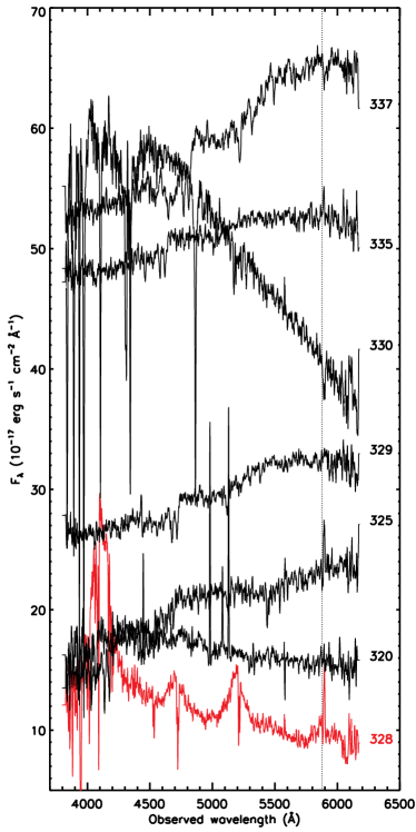
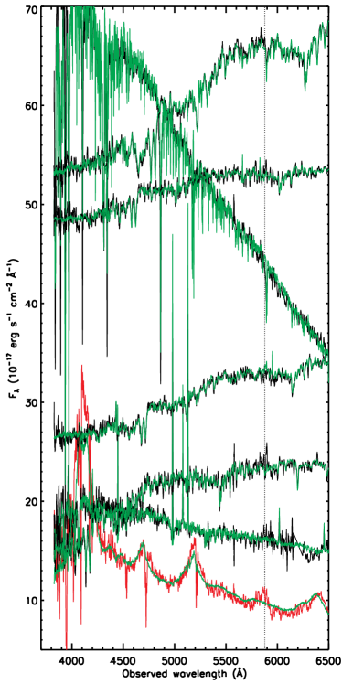
Figure 11: Systematics check for instrumental problems. (Left) Co-added blue-side spectrum for SDSS J1204+3518 (shown in red) compared to spectra taken by other fibers (shown in black; fiber numbers are labeled next to each spectrum) on the same plate in the same night. (Right) Co-added and blue–red stitched spectrum for SDSS J1204+3518 (shown in red) compared to those for other fiber spectra (shown in black). Overplotted are the best-fit models (shown in green) from the SDSS automatic spectroscopic pipeline. Only SDSS J1204+3518 shows significant residual emission around the expected observed wavelength of N III] $\lambda$1750 (denoted by dotted lines) between the data and the pipeline models (that do not account for N III] $\lambda$1750). The SDSS automatic pipeline provides a poor fit for SDSS J1204+3518 largely due to the significant N III] $\lambda$1750 emission, which is not being accounted for in the template (because this feature is much weaker for normal quasars). All spectra (not model) have been smoothed by a 4-pixel boxcar for better clarity. Spectra for the comparison fibers are offset vertically for display purposes.

References

- Adelman-McCarthy et al. (2007) Adelman-McCarthy, J. K., Agüeros, M. A., Allam, S. S., et al. 2007, ApJS, 172, 634
- Arcavi et al. (2014) Arcavi, I., Gal-Yam, A., Sullivan, M., et al. 2014, ApJ, 793, 38
- Auchettl et al. (2017) Auchettl, K., Guillochon, J., & Ramirez-Ruiz, E. 2017, ApJ, 838, 149
- Auchettl et al. (2018) Auchettl, K., Ramirez-Ruiz, E., & Guillochon, J. 2018, ApJ, 852, 37
- Bade et al. (1996) Bade, N., Komossa, S., & Dahlem, M. 1996, A&A, 309, L35
- Baldwin et al. (2003a) Baldwin, J. A., Ferland, G. J., Korista, K. T., Hamann, F., & Dietrich, M. 2003a, ApJ, 582, 590
- Baldwin et al. (2003b) Baldwin, J. A., Hamann, F., Korista, K. T., et al. 2003b, ApJ, 583, 649
- Batra & Baldwin (2014) Batra, N. D., & Baldwin, J. A. 2014, MNRAS, 439, 771
- Bentz et al. (2004) Bentz, M. C., Hall, P. B., & Osmer, P. S. 2004, AJ, 128, 561
- Bentz & Osmer (2004) Bentz, M. C., & Osmer, P. S. 2004, AJ, 127, 576
- Blanchard et al. (2017) Blanchard, P. K., Nicholl, M., Berger, E., et al. 2017, ApJ, 843, 106
- Blandford & Znajek (1977) Blandford, R. D., & Znajek, R. L. 1977, Monthly Notices of the Royal Astronomical Society, 179, 433. http://dx.doi.org/10.1093/mnras/179.3.433
- Brown et al. (2017) Brown, J. S., Holoien, T. W.-S., Auchettl, K., et al. 2017, MNRAS, 466, 4904
- Brown et al. (2016) Brown, J. S., Shappee, B. J., Holoien, T. W.-S., et al. 2016, MNRAS, 462, 3993
- Brown et al. (2018) Brown, J. S., Kochanek, C. S., Holoien, T. W.-S., et al. 2018, MNRAS, 473, 1130
- Cenko et al. (2012) Cenko, S. B., Krimm, H. A., Horesh, A., et al. 2012, ApJ, 753, 77
- Cenko et al. (2016) Cenko, S. B., Cucchiara, A., Roth, N., et al. 2016, ApJ, 818, L32
- Collin & Zahn (1999) Collin, S., & Zahn, J.-P. 1999, A&A, 344, 433
- Dawson et al. (2013) Dawson, K. S., Schlegel, D. J., Ahn, C. P., et al. 2013, AJ, 145, 10
- Dickey & Lockman (1990) Dickey, J. M., & Lockman, F. J. 1990, ARA&A, 28, 215
- Dietrich et al. (2003) Dietrich, M., Hamann, F., Shields, J. C., et al. 2003, ApJ, 589, 722
- Dong et al. (2016) Dong, S., Shappee, B. J., Prieto, J. L., et al. 2016, Science, 351, 257
- Drake et al. (2009) Drake, A. J., Djorgovski, S. G., Mahabal, A., et al. 2009, ApJ, 696, 870
- Erb et al. (2006) Erb, D. K., Shapley, A. E., Pettini, M., et al. 2006, ApJ, 644, 813
- Ferrarese & Merritt (2000) Ferrarese, L., & Merritt, D. 2000, ApJ, 539, L9
- Friaca & Terlevich (1998) Friaca, A. C. S., & Terlevich, R. J. 1998, MNRAS, 298, 399
- Gallegos-Garcia et al. (2018) Gallegos-Garcia, M., Law-Smith, J., & Ramirez-Ruiz, E. 2018, ArXiv e-prints 1801.03497, arXiv:1801.03497
- Gebhardt et al. (2000) Gebhardt, K., Bender, R., Bower, G., et al. 2000, ApJ, 539, L13
- Gezari et al. (2017) Gezari, S., Cenko, S. B., & Arcavi, I. 2017, ApJ, 851, L47
- Gibson et al. (2008) Gibson, R. R., Brandt, W. N., & Schneider, D. P. 2008, ApJ, 685, 773
- Godoy-Rivera et al. (2017) Godoy-Rivera, D., Stanek, K. Z., Kochanek, C. S., et al. 2017, MNRAS, 466, 1428
- Graham (2016) Graham, A. W. 2016, Galactic Bulges, 418, 263
- Guillochon & Ramirez-Ruiz (2013) Guillochon, J., & Ramirez-Ruiz, E. 2013, ApJ, 767, 25
- Hamann & Ferland (1993) Hamann, F., & Ferland, G. 1993, ApJ, 418, 11
- Hills (1975) Hills, J. G. 1975, Nature, 254, 295
- Holoien et al. (2014) Holoien, T. W.-S., Prieto, J. L., Bersier, D., et al. 2014, MNRAS, 445, 3263
- Holoien et al. (2016a) Holoien, T. W.-S., Kochanek, C. S., Prieto, J. L., et al. 2016a, MNRAS, 455, 2918
- Holoien et al. (2016b) —. 2016b, MNRAS, 463, 3813
- Jiang et al. (2007) Jiang, L., Fan, X., Ivezić, Ž., et al. 2007, ApJ, 656, 680
- Jiang et al. (2008) Jiang, L., Fan, X., & Vestergaard, M. 2008, ApJ, 679, 962
- Jiang et al. (2016) Jiang, Y.-F., Guillochon, J., & Loeb, A. 2016, ApJ, 830, 125
- Kellermann et al. (1989) Kellermann, K. I., Sramek, R., Schmidt, M., Shaffer, D. B., & Green, R. 1989, AJ, 98, 1195
- Kochanek (2016a) Kochanek, C. S. 2016a, MNRAS, 458, 127
- Kochanek (2016b) —. 2016b, MNRAS, 461, 371
- Kollmeier et al. (2017) Kollmeier, J. A., Zasowski, G., Rix, H.-W., et al. 2017, ArXiv e-prints 1711.03234, arXiv:1711.03234
- Komossa & Greiner (1999) Komossa, S., & Greiner, J. 1999, A&A, 349, L45
- Kormendy & Ho (2013) Kormendy, J., & Ho, L. C. 2013, ARA&A, 51, 511
- Law et al. (2016) Law, D. R., Cherinka, B., Yan, R., et al. 2016, AJ, 152, 83
- Law et al. (2009) Law, N. M., Kulkarni, S. R., Dekany, R. G., et al. 2009, PASP, 121, 1395
- Leloudas et al. (2016) Leloudas, G., Fraser, M., Stone, N. C., et al. 2016, Nature Astronomy, 1, 0002
- Lin et al. (2015) Lin, D., Maksym, P. W., Irwin, J. A., et al. 2015, ApJ, 811, 43
- Lusso & Risaliti (2016) Lusso, E., & Risaliti, G. 2016, ApJ, 819, 154
- MacLeod et al. (2010) MacLeod, C. L., Ivezić, Ž., Kochanek, C. S., et al. 2010, ApJ, 721, 1014
- MacLeod et al. (2012) MacLeod, M., Guillochon, J., & Ramirez-Ruiz, E. 2012, ApJ, 757, 134
- Maiolino et al. (2008) Maiolino, R., Nagao, T., Grazian, A., et al. 2008, A&A, 488, 463
- McConnachie et al. (2016) McConnachie, A., Babusiaux, C., Balogh, M., et al. 2016, ArXiv e-prints 1606.00043, arXiv:1606.00043
- Morganson et al. (2014) Morganson, E., Burgett, W. S., Chambers, K. C., et al. 2014, ApJ, 784, 92
- Nagao et al. (2006) Nagao, T., Marconi, A., & Maiolino, R. 2006, A&A, 447, 157
- Osmer (1980) Osmer, P. S. 1980, ApJ, 237, 666
- Osterbrock (1989) Osterbrock, D. E. 1989, Astrophysics of gaseous nebulae and active galactic nuclei (Research supported by the University of California, John Simon Guggenheim Memorial Foundation, University of Minnesota, et al. Mill Valley, CA, University Science Books, 1989, 422 p.)
- Peterson (1988) Peterson, B. M. 1988, PASP, 100, 18
- Peterson (1997) —. 1997, An Introduction to Active Galactic Nuclei
- Pfeffermann et al. (1987) Pfeffermann, E., Briel, U. G., Hippmann, H., et al. 1987, in Proc. SPIE, Vol. 733, Soft X-ray optics and technology, 519
- Rees (1988) Rees, M. J. 1988, Nature, 333, 523
- Richards et al. (2006) Richards, G. T., Lacy, M., Storrie-Lombardi, L. J., et al. 2006, ApJS, 166, 470
- Romano et al. (2002) Romano, D., Silva, L., Matteucci, F., & Danese, L. 2002, MNRAS, 334, 444
- Rosen et al. (2016) Rosen, S. R., Webb, N. A., Watson, M. G., et al. 2016, A&A, 590, A1
- Rumbaugh et al. (2018) Rumbaugh, N., Shen, Y., Morganson, E., et al. 2018, ApJ, 854, 160
- Schneider et al. (2007) Schneider, D. P., Hall, P. B., Richards, G. T., et al. 2007, AJ, 134, 102
- Schneider et al. (2010) Schneider, D. P., Richards, G. T., Hall, P. B., et al. 2010, AJ, 139, 2360
- SDSS Collaboration et al. (2016) SDSS Collaboration, Albareti, F. D., Allende Prieto, C., et al. 2016, ArXiv e-prints 1608.02013, arXiv:1608.02013
- Sesar et al. (2011) Sesar, B., Stuart, J. S., Ivezić, Ž., et al. 2011, AJ, 142, 190
- Shen (2013) Shen, Y. 2013, Bulletin of the Astronomical Society of India, 41, 61
- Shen & Liu (2012) Shen, Y., & Liu, X. 2012, ApJ, 753, 125
- Shen et al. (2011) Shen, Y., Richards, G. T., Strauss, M. A., et al. 2011, ApJS, 194, 45
- Shields (1976) Shields, G. A. 1976, ApJ, 204, 330
- Sikora et al. (2007) Sikora, M., Stawarz, Ł., & Lasota, J.-P. 2007, ApJ, 658, 815
- Tadhunter et al. (2017) Tadhunter, C., Spence, R., Rose, M., Mullaney, J., & Crowther, P. 2017, Nature Astronomy, 1, 0061
- Tremaine et al. (2002) Tremaine, S., Gebhardt, K., Bender, R., et al. 2002, ApJ, 574, 740
- Tremonti et al. (2004) Tremonti, C. A., Heckman, T. M., Kauffmann, G., et al. 2004, ApJ, 613, 898
- Vestergaard & Osmer (2009) Vestergaard, M., & Osmer, P. S. 2009, ApJ, 699, 800
- Vestergaard & Peterson (2006) Vestergaard, M., & Peterson, B. M. 2006, ApJ, 641, 689
- Voges et al. (1999) Voges, W., Aschenbach, B., Boller, T., et al. 1999, A&A, 349, 389
- Voges et al. (2000) —. 2000, IAUC, 7432, 3
- Wang et al. (2011) Wang, J., Fabbiano, G., Risaliti, G., et al. 2011, ApJ, 729, 75
- White et al. (1997) White, R. L., Becker, R. H., Helfand, D. J., & Gregg, M. D. 1997, ApJ, 475, 479
- Yang et al. (2017) Yang, C., Wang, T., Ferland, G. J., et al. 2017, ApJ, 846, 150
- York et al. (2000) York, D. G., Adelman, J., Anderson, Jr., J. E., et al. 2000, AJ, 120, 1579
- Young et al. (2009) Young, M., Elvis, M., & Risaliti, G. 2009, ApJS, 183, 17