Self-trapping and acceleration of ions in laser-driven relativistically transparent plasma

Abstract

Self-trapping and acceleration of ions in laser-driven relativistically transparent plasma are investigated with the help of particle-in-cell simulations. A theoretical model based on ion wave breaking is established in describing ion evolution and ion trapping. The threshold for ion trapping is identified. Near the threshold ion trapping is self-regulating and stops when the number of trapped ions is large enough. The model is applied to ion trapping in three-dimensional geometry. Longitudinal distributions of ions and the electric field near the wave breaking point are derived analytically in terms of power-law scalings. The areal density of trapped charge is obtained as a function of the strength of ion wave breaking, which scales with target density for fixed laser intensity. The results of the model are confirmed by the simulations.

I Introduction

Laser-driven plasma-based ion acceleration has attracted substantial interest due to its potential applications in many areas rev1 ; app1 ; app2 ; app3 , including medical treatment of cancer, matter detection, fast ignition in inertial confinement fusion, nuclear physics, and high energy physics.

Recent developments of ultra-intense laser technology have opened new options for generating high energy ion beams hb ; rpa ; piston ; robinson ; weng ; rita ; sasl ; sasl3 ; iwba . An ultra-intense laser pulse is capable of producing a localized charge-separation field in the region behind of laser front. Ions trapped in the field are accelerated to velocities far beyond the velocity of the laser front. In order to achieve high energy ion acceleration, it is necessary to make the accelerating field propagate as fast as possible. However, when it is too fast background ions cannot be self-trapped. There must exist a threshold condition where ion trapping initiates. For a given laser pulse the most energetic ions are produced under the threshold condition.

Here we focus on ion trapping and acceleration near the threshold condition. This has not been studied in sufficient detail so far. In previous work iwba we have pointed out that ion trapping near the threshold condition is caused by ion wave breaking. In the present paper, with the help of particle-in-cell (PIC) simulations, we develop a theoretical model to investigate the ion trapping in more detail. We demonstrate that the ion trapping initiates with the transition from fluid-like to kinetic behaviour, accompanied by the transition from oscillatory to self-trapping dynamics, as well as the transition from non-crossing to crossing trajectories. It happens in near-critical ncdt1 ; ncdt2 ; ncdt3 ; ncdt4 relativistically transparent trans plasma. The interesting point is that this trapping process is self-regulating and stops when the number of trapped ions is large enough. This is significantly different from ion acceleration regimes in opaque plasma, such as hole boring hb , laser piston piston , and radiation pressure acceleration for thin foils rpa , where all ions in the laser focuses are accelerated. This results in high-quality ion beams with low energy spread and beam emittance. The number of trapped ions can be controlled by external parameters like laser intensity and target density. It allows to design robust and controllable laser-plasma ion accelerators.

A few efforts have been made previously on ion acceleration in laser-driven plasma waves or wave-like structures in near-critical relativistically transparent plasma. In Ref. ionwake , O. Shorokhov and A. Pukhov have proposed the so-called ion wakefield acceleration mechanism in which ions are trapped in an electron plasma wave and accelerated. Ion acceleration in bubble regime in 3D geometry has been investigated in Ref. ionbub . Ion acceleration in laser-driven comoving electrostatic field in inhomogeneous plasma has been studied in the scheme of relativistically induced transparency acceleration rita . In all these works, the fields that trap and accelerate ions are produced by the oscillations of electrons. In order to maintain the fields, stable and positively charged backgrounds are required. Two-component plasma targets are used in these works where a large proportion of heavier (larger mass-to-charge ratio) ions compose the background and a small proportion of lighter ions are trapped and accelerated. This makes a high demand on target preparing and limits their applications. In our work, background ions are significantly disturbed and ion waves are excited. The ion wave survives even though an electron wave is completely destroyed. Therefore, ion acceleration via ion wave breaking works well even when the plasma is composed of only one kind of ions.

The present paper is organized as follows. In Sec. II, we investigate ion trapping via ion wave breaking based on a 1D model. In Sec. III, we apply the 1D model to estimate ion trapping in practical 3D geometry. In Sec. IV, we compare the model predictions with 3D PIC simulations. Conclusions are given in Sec. V.

II 1D model of ion wave breaking

II.1 Electron wave and ion wave

We follow the pioneering work of A. I. Akhiezer and R. V. Polovin Akhiezer . We consider a one-dimensional plane plasma wave (longitudinal oscillation) propagating in an uniform unmagnetized plasma along $z$-direction with phase velocity $v_{\rm{ph}}$. The difference here is that we take ion motion into account. We assume the plasma is composed of electrons and one kind of ions, having number densities $n_{e}$ and $n_{i}$, respectively. The plasma is described by the equations of motion and continuity for electrons,

$$\left(\frac{\partial}{\partial t}+v_{e}\frac{\partial}{\partial z}\right)(m_{e}\gamma_{e}v_{e}) = -eE_{z},$$ (1)

$$\frac{\partial n_{e}}{\partial t}+\frac{\partial}{\partial z}(n_{e}v_{e}) = 0,$$ (2)

and ions,

$$\left(\frac{\partial}{\partial t}+v_{i}\frac{\partial}{\partial z}\right)(m_{i}\gamma_{i}v_{i}) = q_{i}E_{z},$$ (3)

$$\frac{\partial n_{i}}{\partial t}+\frac{\partial}{\partial z}(n_{i}v_{i}) = 0,$$ (4)

respectively, and Poisson’s equation footnote0 ,

$$\frac{\partial}{\partial z}E_{z} = \frac{1}{\epsilon_{0}}(q_{i}n_{i}-en_{e}),$$ (5)

where $\gamma_{e,i}=1/\sqrt{1-\beta_{e,i}^{2}}$, $\beta_{e,i}=v_{e,i}/c$, $v_{e}$ ($v_{i}$) denotes the electron (ion) velocity, $c$ the light speed in vacuum, $e$ ($q_{i}$) the electron (ion) charge, $m_{e}$ ($m_{i}$) the electron (ion) mass, $E_{z}$ the longitudinal electric field, and $\epsilon_{0}$ the vacuum permittivity.

If the velocity $v_{\rm{ph}}$ is constant, all the variables can be written as functions of $\zeta=\omega_{i}(z/v_{\rm{ph}}-t)$ (see Ref. Akhiezer ), instead of $z$ and $t$ separately, where $\omega_{i}=\sqrt{q_{i}en_{0}/m_{i}\epsilon_{0}}$ is the ion oscillation frequency, $e$ denotes the electron charge, and $n_{0}$ the initial plasma density. We look for stationary wave solutions $n_{e,i}(\xi)$, $\beta_{e,i}(\xi)$, and $E_{z}(\xi)$. Introducing dimensionless quantities $\tilde{n}_{e}=n_{e}/n_{0},$ $\tilde{n}_{i}=q_{i}n_{i}/en_{0},$ and $\tilde{E}=E_{z}/E_{0}$, where $E_{0}=m_{i}c\omega_{i}/q_{i}$, Eqs. (1-5) transform into

$$(1-\beta_{e}/\beta_{\rm{ph}})\frac{d\gamma_{e}\beta_{e}}{d\zeta} = \mu\tilde{E},$$ (6)

$$\frac{d}{d\zeta}\left(\tilde{n}_{e}-\tilde{n}_{e}\beta_{e}/\beta_{\rm{ph}}\right) = 0,$$ (7)

$$(1-\beta_{i}/\beta_{\rm{ph}})\frac{d\gamma_{i}\beta_{i}}{d\zeta} = -\tilde{E},$$ (8)

$$\frac{d}{d\zeta}\left(\tilde{n}_{i}-\tilde{n}_{i}\beta_{i}/\beta_{\rm{ph}}\right) = 0,$$ (9)

$$\frac{d\tilde{E}}{d\zeta} = \beta_{\rm{ph}}(\tilde{n}_{i}-\tilde{n}_{e}),$$ (10)

where $\beta_{\rm{ph}}=v_{\rm{ph}}/c$, and $\mu=(m_{i}/m_{e})/(q_{i}/e)$. The densities,

$$\tilde{n}_{e} = \frac{1}{1-\beta_{e}/\beta_{\rm{ph}}},$$ (11)

$$\tilde{n}_{i} = \frac{1}{1-\beta_{i}/\beta_{\rm{ph}}},$$ (12)

are obtained directly from Eqs. (7, 9) since $\tilde{n}_{e}\equiv\tilde{n}_{i}\equiv 1$ for unperturbed plasma ($\beta_{e}\equiv\beta_{i}\equiv 0$).

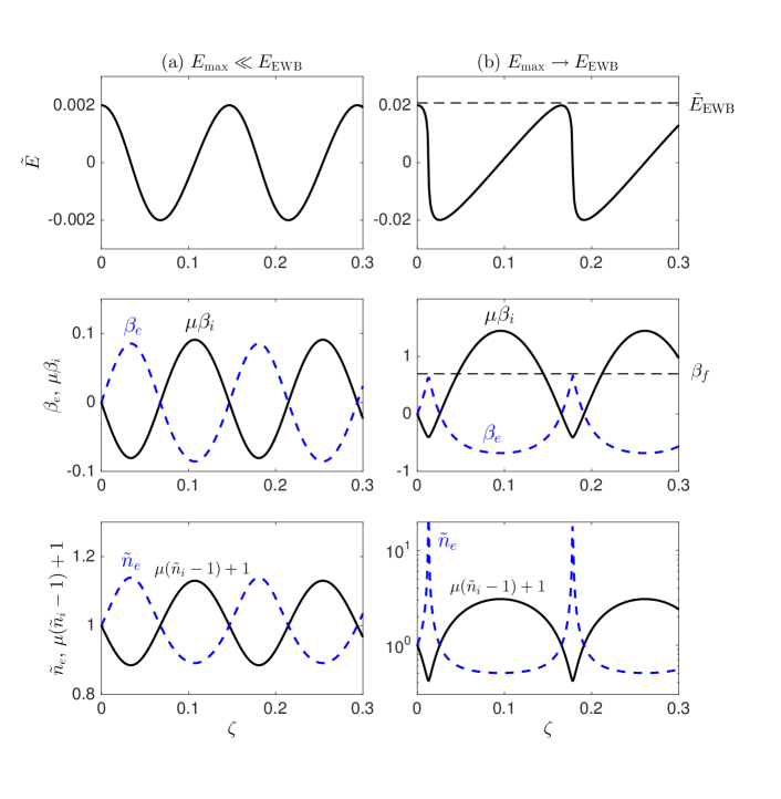
Figure 1: Results of (top panels) longitudinal electric field $\tilde{E}$, (middle panels) electron (ion) velocity $\beta_{e}$ ($\beta_{i}$) and (lower panels) density $\tilde{n}_{e}$ ($\tilde{n}_{i}$), by numerically solving Eqs. (6, 8, 10, 11, 12) with $\beta_{\rm{ph}}=0.7$, and (a) $E_{\rm{max}}=0.002$, (b) $E_{\rm{max}}=0.020$, where $\mu=1836$ for hydrogen plasma. The electron wave breaking field $E_{\rm{EWB}}=0.021$ is calculated according to Eq. (13). The electron wave is accompanied by an ion wave.

By numerically solving Eqs. (6, 8, 10, 11, 12) with $\beta_{\rm{ph}}=0.7$ and boundary conditions $\beta_{e}(0)=0$, $\beta_{i}(0)=0$, and $\tilde{E}_{z}(0)=0.002$, the distributions of electrons, ions, and the longitudinal electric field are shown in Fig. 1 (a). It is shown that the electron wave is accompanied by an ion wave. The electron wave, the ion wave, and the longitudinal electric field are all oscillating sinusoidally. The ion wave peaks at the electron wave valley where $E_{z}$ changes sign from negative to positive. As $\mu\gg 1$, the amplitude of the ion wave is far smaller than that of the electron wave.

As is well-known Akhiezer ; dawson ; ewbrev , the amplitude of plasma wave can be characterized by the maximum longitudinal electric field $E_{\rm{max}}$, and there exists a threshold field for electron wave breaking (here we denote it by $E_{\rm{EWB}}$), beyond which the fluid-like behaviour of electrons breaks down and there is no solution for Eqs. (6, 8, 10, 11, 12). When $\mu\gg 1$, the threshold field in Ref. Akhiezer is reproduced footnote1 as

$$\tilde{E}_{\rm{EWB}}=\sqrt{2(\gamma_{\rm{ph}}-1)/\mu},$$ (13)

where $\gamma_{\rm{ph}}=1/\sqrt{1-\beta_{\rm{ph}}^{2}}$. Figure 1 (b) shows the results when $E_{\rm{max}}$ approaches $E_{\rm{EWB}}$. As is also well-known, the electron wave becomes strongly nonlinear, and the electric field becomes a sawtooth-like wave. The interesting thing is that the ion wave is also strongly nonlinear, instead of sinusoidal-like, although its amplitude is still very small.

II.2 Ion wave breaking

II.2.1 Equations of ions

A plasma wave can be produced by propagating a laser pulse in plasma. In 1D geometry, the electric field and plasma along the laser propagation direction is well described by Eqs. (6,8,10,11,12) when the maximum electric field satisfies $E_{\rm{max}}<E_{\rm{EWB}}$. When the laser drive is strong enough so that $E_{\rm{max}}>E_{\rm{EWB}}$, self-trapping of electrons happens, and the fluid model for electrons breaks down. However, ions still behave like a fluid and Eqs. (3,4,5) are still valid, as long as there is no self-trapping of ions.

We denote the propagating velocity of the laser front by $v_{f}$. If $v_{f}$ is constant, and the plasma is stationary in the frame comoving with $v_{f}$, then, similar to that in Sec. II A, all the variables can be written as functions of $\xi=\omega_{i}(z/v_{f}-t)$, and Eqs. (3,4,5) become,

$$(1-\beta_{i}/\beta_{f})\frac{d\gamma_{i}\beta_{i}}{d\xi} = -\tilde{E},$$ (14)

$$\tilde{n}_{i} = \frac{1}{1-\beta_{i}/\beta_{f}},$$ (15)

$$\frac{d\tilde{E}}{d\xi} = \beta_{f}(\tilde{n}_{i}-\tilde{n}_{e}),$$ (16)

where $\beta_{f}=v_{f}/c$.

II.2.2 1D PIC simulation

In order to investigate the general features of ion evolution under the condition of $E_{\rm{max}}>E_{\rm{EWB}}$, a 1D PIC simulation has been carried out by using the plasma simulation code (PSC) psc . The simulation makes use of a constant laser pulse with circular polarization (similar features exist for linearly polarized cases) and laser intensity $I_{L}=5\times 10^{21}\rm{W/cm^{2}}$ (laser amplitude $a_{0}=44$ for wavelength $1\rm{\mu m}$, where $a_{0}=eE_{L}/m_{e}c\omega_{L}$, $E_{L}$ denotes the laser electric field, and $\omega_{L}$ the laser frequency) of semi-infinite duration, and a sine-squared front edge rising over 5 laser periods. The initial plasma density rises linearly from $z=5\mu m$ to $z=6\mu m$ and then keeps constant as $n_{0}=0.2n_{c}$ until the end of the simulation box at $z=100\mu m$, where $n_{c}=m_{e}\omega_{L}^{2}\epsilon_{0}/e^{2}$ is the critical plasma density. The plasma is composed of electrons and protons. A resolution of 500 cells per micron and 20 particles per species per cell is used. The initial temperature is 100 eV for electrons and 0 for ions.

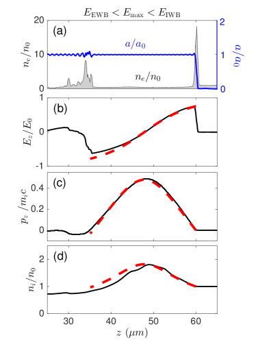
Figure 2: A snapshot of (a) laser amplitude ($a/a_{0}$, blue line), electron density ($\tilde{n}_{e}$, grey area), (b) electric field ($\tilde{E_{z}}$, black solid line), (c) ion momentum ($p_{z}/m_{i}c$, black solid line), and (d) ion density ($\tilde{n}_{i}$, black solid line), from a 1D PIC simulation with the laser amplitude $a_{0}=44$ and initial plasma density $n_{0}=0.2n_{c}$. An ion wave survives even though an electron wave does not exist. The results of the model (red dashed lines) are obtained by numerically solving Eqs. (14-17) with quantities $\beta_{f}\sim 0.96$, $v_{b}\sim v_{i}(z=60\mu m)\sim 0$, $E_{\rm{max}}\sim E_{z}(z=60\mu m)\sim 0.75E_{0}$, and $\tilde{n}_{el}\sim 0.5$ in the range of $35\mu m<z<60\mu m$, observed in the simulation. The results are under the condition of $E_{\rm{EWB}}<E_{\rm{max}}<E_{\rm{IWB}}$, where $E_{\rm{EWB}}=0.05E_{0}$ is calculated according to Eq. (13) by assuming $\beta_{\rm{ph}}=\beta_{f}$, while $E_{\rm{IWB}}=2.42E_{0}$ is calculated according to Eq. (20).

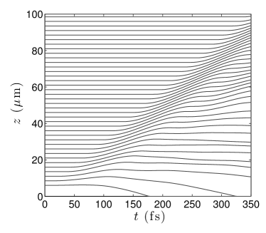
Figure 3: Trajectories of ions with different initial positions for the 1D simulation shown in Fig. 2. Ions show fluid-like behaviour.

The simulation results are shown in Fig. 2. The laser pulse pushes electrons and piles them up at the laser front, forming a leading electron layer, and leaving a region behind of the laser front with relatively low electron density that is almost constant in the range of $35\mu m<z<60\mu m$. A charge-separation field $E_{z}$ is then produced. Ions first acquire velocity in laser direction in the region where $E_{z}>0$, but then loose it again in the region where $E_{z}<0$ (see Fig. 2(b,c)). Profiles of ion velocity and density are similar to that Fig. 1 (b), when the electron wave is strongly nonlinear, except that in Fig. 2 the oscillation lasts only one period and the amplitudes are much larger. Furthermore, trajectories of ions at different initial positions are plotted in Fig. 3. It is clearly shown that ions still behave like a fluid and there is no trajectory crossing. In this sense, we can say that the ion wave survives in the region just behind of the laser front.

II.2.3 Electron density

The ion wave is coupled with the electron density $\tilde{n}_{e}$ via Poisson’s equation (Eq. (16)). Since the fluid behaviour of electrons breaks down, $\tilde{n}_{e}$ cannot be obtained from fluid equations now. Fortunately, ions are much heavier than electrons. Thus, ions evolve slowly compared to electrons and ion motion is insensitive to the fast variations of the electron density. Therefore, for simplicity, we approximate the electron density as a step function,

$${n}_{e}=\begin{cases}n_{0},&\xi>\xi_{a};\\ {n}_{ep},&\xi_{b}<\xi<\xi_{a};\\ {n}_{el},&\xi_{c}<\xi<\xi_{b},\\ \rm{not~{}of~{}concern},&\xi<\xi_{c},\end{cases}$$ (17)

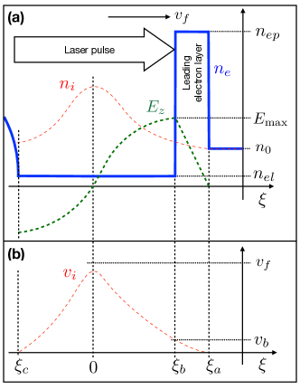
Figure 4: Schematic figure of ion dynamics under the condition of $E_{\rm{EWB}}<E_{\rm{max}}<E_{\rm{IWB}}$, modelling the simulation results of Fig. 2. Plot (a): electron density (thick blue line), ion density (thin red line), and electric field (green dashed line). Plot (b): ion velocity (thin red line). The laser front propagates forward with front velocity $v_{f}$. The electron density distribution is modelled as $n_{ep}$ for $\xi_{b}<\xi<\xi_{a}$ and $n_{el}$ for $\xi_{c}<\xi<\xi_{b}$, where $\xi_{c}$ satisfies $v_{i}(\xi_{c})=0$ and $E_{z}(\xi_{c})<0$. The electric field $E_{z}$ peaks at $\xi_{b}$, i.e., $E_{\rm{max}}=E_{z}(\xi_{b})$). The ion velocity at $\xi_{b}$ is smaller than the laser front velocity ($v_{b}<v_{f}$). We chose $\xi=0$ as the point where ion velocity and density peak and $E_{z}$ changes sign.

where $\xi_{c}$ is chosen as the point where ions are decelerated to zero velocity for the first time ($\beta_{i}(\xi_{c})=0$ and $E_{z}(\xi_{c})<0$), $\xi_{a}$ and $\xi_{b}$ denote the boundaries of the leading electron layer. The modelled electron density is illustrated in Fig. 4. Then the charge-separation field peaks at $\xi_{b}$, i.e., $E(\xi_{b})=E_{\rm{max}}$. The ion velocity at $\xi_{b}$ is denoted by $v_{b}$. It is smaller than the laser front velocity ($v_{b}<v_{f}$). For simplicity, we chose $\xi=0$ as the point where the ion velocity peaks. Then, at the point $\xi=0$, the ion density also peaks (see Eq. (15) and the electric field changes sign from negative to positive (according to Eq. (14) and Eq. (16), $\tilde{E}(0)=0$ and $d\tilde{E}/d\xi|_{\xi=0}>0$). For $\xi<\xi_{c}$, the electron density is too complex but not important for ion trapping and acceleration. Thus, it is not of concern in our model. Higher order modifications of the electron density may give more details. Nevertheless, this approximation works very well, especially when $n_{el}\ll n_{i}$.

Results of the model of the electric field $E_{z}$, the ions momentum $p_{z}$, and the ion density $n_{i}$ are shown in Fig. 2 (b,c,d), denoted by red dashed lines. It is seen that the curves from the model with parameters observed in the simulation fit the simulation results very well.

If there exists an electron wave, as is well-known, the phase velocity of the electron wave should equal the laser front velocity, i.e., $\beta_{\rm{ph}}=\beta_{f}\sim 0.96$. However, in this case, according to Eq. (13), one has $\tilde{E}_{\rm{EWB}}=0.05<\tilde{E}_{\rm{max}}$. Thus, there is no electron wave anymore. This confirms that an ion wave can survive even though an electron wave does not exist.

II.2.4 Ion wave breaking threshold

Similar to Eq. (13), there exists a threshold field for ion wave breaking as well. Combining Eqs. (14,15,16), we obtain

$$\frac{d}{d\xi}\left(\frac{\tilde{E}^{2}}{2}+\beta_{f}\gamma_{i}\beta_{i}+\tilde{n}_{e}\gamma_{i}(1-\beta_{f}\beta_{i})\right)=0.$$ (18)

Integrating Eq. (18) from $\xi=0$ to $\xi=\xi_{b}$, we find the maximum electric field,

$$\tilde{E}_{\rm{max}}=\sqrt{2\beta_{f}(1-\tilde{n}_{el})(\gamma_{i}(0)\beta_{i}(0)-\gamma_{b}\beta_{b})+2\tilde{n}_{el}(\gamma_{i}(0)-\gamma_{b})},$$ (19)

where $\beta_{b}=v_{b}/c$, and $\gamma_{b}=1/\sqrt{1-\beta_{b}^{2}}$. When the ion velocity peak $\beta_{i}(0)$ equals the velocity of the laser front $\beta_{f}$, the maximum electric field $E_{\rm{max}}$ marks the threshold of ion wave breaking,

$$\tilde{E}_{\rm{IWB}}=\beta_{f}\sqrt{2\gamma_{f}(1-\delta)},$$ (20)

where

$$\delta=\frac{\tilde{n}_{el}}{\beta_{f}^{2}\gamma_{f}^{2}}(\gamma_{b}\gamma_{f}(1-\beta_{b}\beta_{f})-1)+\frac{\beta_{b}\gamma_{b}}{\beta_{f}\gamma_{f}},$$

and $\gamma_{f}=1/\sqrt{1-\beta_{f}^{2}}$.

When $\tilde{E}_{\rm{max}}>\tilde{E}_{\rm{IWB}}$, incoming ions are accelerated to velocities equal to the laser front velocity at points $\xi>0$, where the electric field is positive ($E_{z}>0$). Then these ions will be further accelerated. In the frame comoving with the laser front, they are reflected. This is a process of self-injection of ions into the accelerating field. Then the ions are trapped and further accelerated. In this condition, the fluid-like behaviour of ions breaks down, and there is no solution of Eqs. (14,15,16).

For the simulation shown in Fig. 2, with $\beta_{f}\sim 0.96$, $\tilde{n}_{el}\sim 0.5$, and $\beta_{b}\sim 0$, one has the threshold field $E_{\rm{IWB}}=2.4E_{0}$. While the observed maximum charge-separation field in the simulation is $E_{\rm{max}}\sim 0.75E_{0}$. It is still smaller than the threshold value ($E_{\rm{max}}<E_{\rm{IWB}}$). This explains the fluid-like behaviour of ions in the simulation, as is clearly seen in Figs. (2,3).

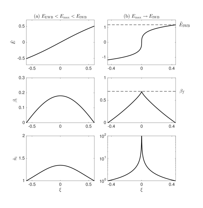
Figure 5: Column (a): Results of the model of (top panels) electric field $\tilde{E}$, (middle panels) ion velocity $\beta_{i}$, and (lower panels) ion density $\tilde{n}_{i}$, by numerically solving Eqs. (14-17) with $\tilde{E}(0)=0$, $\beta_{i}(0)=0.18$, and the parameters $\beta_{f}=0.7$, $n_{el}=0$, $v_{b}=0$. Column (b): The same as those in (a) except $\beta_{i}(0)\to\beta_{f}$. The results are under the condition of $\tilde{E}_{\rm{EWB}}<\tilde{E}_{\rm{max}}\leq\tilde{E}_{\rm{IWB}}$, where $\tilde{E}_{\rm{EWB}}=0.02$ is calculated according to Eq. (13) by assuming $\beta_{\rm{ph}}=\beta_{f}$, while $\tilde{E}_{\rm{IWB}}=1.2$ is calculated according to Eq. (20).

Numerical solutions of Eqs. (14,15,16,17) with different $E_{\rm{max}}$ are shown in Fig. 5. A weak ion wave is seen in Fig. 5 (a), in which $E_{\rm{max}}$ is far smaller than $E_{\rm{IWB}}$. Fig. 5 (b) shows a near breaking ion wave, with $E_{\rm{max}}\simeq E_{\rm{IWB}}$. In this case, at $\xi=0$, the ion density diverges, and the gradient of $\tilde{E}$ becomes infinite. It is essentially similar to the electron density and electric field in the case of electron wave breaking (see, e.g., Ref. dawson ).

II.3 Ion trapping

II.3.1 1D PIC simulation

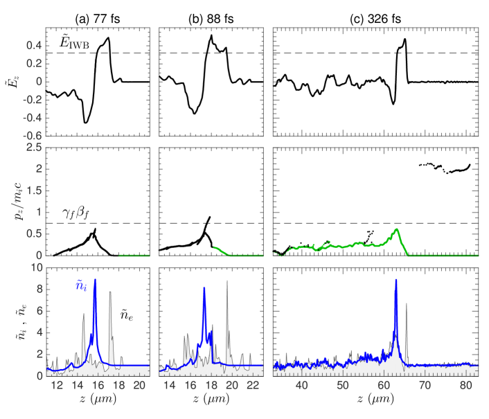
Figure 6: 1D PIC simulation results of longitudinal electric field ($\tilde{E}_{z}$, top panels), ion momentum ($\gamma_{i}\beta_{i}$, middle panels), ion and electron densities ($\tilde{n}_{i}$, blue lines, and $\tilde{n}_{e}$, grey areas, lower panels), at different times (a) 77 fs, (b) 88 fs, (c) 326 fs, with the same laser pulse as that used in Fig. 2 but a higher initial plasma density $n_{0}=3.2n_{c}$. There is no ion wave anymore and ion trapping happens. The horizontal dashed lines in top panels mark the threshold field for ion wave breaking $\tilde{E}_{\rm{IWB}}=0.32$, which is clearly lower than the maximum electric field. In the middle panels, ions initially in the range of $z<18\mu m$ are plotted in black (dark) color, while other ions (initially $z>18\mu m$) are plotted in green (grey). The horizontal dashed lines in the middle panels mark the value of $\gamma_{f}\beta_{f}$. See text for more details.

In order to investigate ion trapping and acceleration under the condition of $E_{\rm{max}}>E_{\rm{IWB}}$, a 1D PIC simulation has been carried out with laser plasma parameters the same as that used in Fig. 2 but a higher initial plasma density $n_{0}=3.2n_{c}$. The simulation results are shown in Fig. 6. At 77 fs (Fig. 6 (a)), a high density electron layer (in the region $17\mu m<z<17.5\mu m$) is produced at the front of the laser pulse (the laser pulse is not shown). The ion density peaks at about $15.7\mu m$. The longitudinal electric field is positive in between the leading electron layer and the ion density peak and negative in the region behind. The maximum ion velocity is very close to the laser front velocity ($\beta_{f}\sim 0.6$). Ion trapping happens around the later time 88 fs (Fig. 6 (b)). The average electron density in the range of $15\mu m<z<19\mu m$ in Fig. 6 (b) lower panel is about $\sim 2n_{0}$. If we apply $\tilde{n}_{el}\sim 2$ to Eq. (20), we have $\tilde{E}_{\rm{IWB}}=0.32$; it is marked in the top panels in Fig. 6 by dashed lines. The maximum laser-driven charge-separation field is found to be $\tilde{E}_{\rm{max}}\sim 0.5$. It is clear that $\tilde{E}_{\rm{max}}>\tilde{E}_{\rm{IWB}}$. The trapped ions are accelerated by the charge-separation field, until they overtake the laser front (Fig. 6 (c)).

In the frame comoving with the laser front ions come into the region behind of the laser front with initial velocity $-v_{f}$, then reflected and overtakes the laser front with velocity $v_{f}$. Therefore, in the laboratory frame, according to the relativistic velocity addition, we have the velocity of the output ions, $\beta_{i,\rm{out}}=2\beta_{f}/(1+\beta_{f}^{2})$, and the kinetic energy iwba ,

$$\mathcal{E}_{i,\rm{out}}=2\gamma_{f}^{2}\beta_{f}^{2}m_{i}c^{2}.$$ (21)

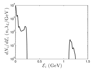
Figure 7: Ion energy spectrum corresponding to the simulation result in Fig. 6 (c).

With $\beta_{f}\sim 0.6$, we have $\mathcal{E}_{i,\rm{out}}\sim 1.1$ GeV. This coincides with the peak of the energy spectrum directly observed from the simulation (Fig. 7).

Finally, the output ions are separated from the untrapped ions, as is shown in Fig. 6 (c) middle panel. It is noticed that all the output ions initially come from the region $z<18\mu m$. On the other hand, all the ions initially in the region $z>18\mu m$ have not been trapped and accelerated. Since the duration of the incident laser pulse is semi-infinite, this reflects that the ion trapping process is self-regulating and self-stops. This results in the peaked energy spectrum shown in Fig. 7.

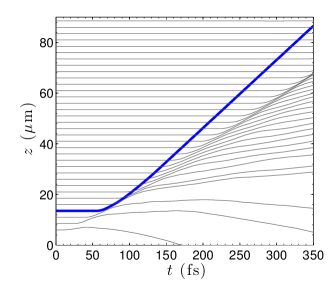
Figure 8: Trajectories of ions with different initial positions for the 1D simulation shown in Fig. 6. The crossing trajectory with initial position $z(t=0)=13.5\mu m$ is highlighted as a thick blue line.

Figure 8 shows trajectories of ions. Different from that in Fig. 3, trajectory crossing happens from $t\sim$ 80 fs onward. The trajectory of an ion initially at $z=13.5\mu m$ (thick blue line) crosses with the trajectories of the ions initially at $z\geq 16\mu m$ one by one. However, the trajectories of untrapped ions (thin black lines) do not cross each other, indicating that the untrapped ions still behave like a fluid.

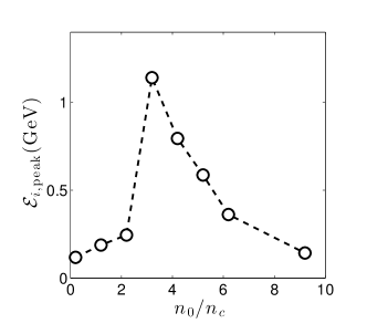
Figure 9: 1D PIC simulation results of peak ion energy ($\mathcal{E}_{i,\rm{peak}}$) with the same laser pulse ($a_{0}=44$) as that used in Fig. 2 and Fig. 6 but different initial plasma densities $n_{0}$.

Peak ion energies for different initial plasma densities are shown in Fig. 9. For $n_{0}\leq 2.2n_{c}$, there is no ion acceleration. They are in the regime of $E_{\rm{max}}<E_{\rm{IWB}}$. The maximum ion velocity is far less than the corresponding laser front velocity. For $n_{0}\geq 3.2n_{c}$, ion trapping happens and ions are accelerated. The peak energy of the output ion beam decreases with the increase of $n_{0}$.

II.3.2 Self-stopping of ion trapping

It is clear that the ion trapping discussed above (Figs. 6-9) happens in relativistically transparent regime. As is well known vrt1 , the laser front velocity in a relativistically transparent plasma is significantly faster than the hole-boring velocity $v_{\rm{hb}}$. This requires that the ion trapping process in relativistically transparent regime has to self-stop. This can be explained by introducing a paradox. For a laser pulse with a long duration ($\tau_{L}\gg(\xi_{a}-\xi_{c})/\omega_{i}$), if the self-trapping process is continuous from the beginning to the end, the total number of the accelerated ions can be estimated as $\mathcal{N}_{i}\sim n_{0}v_{f}\Delta t$, where $\Delta t\sim\tau_{L}/(1-\beta_{f})$ is the interaction time. Then the total ion energy satisfies

$$\mathcal{N}_{i}\mathcal{E}_{i,\rm{out}} = 2n_{0}m_{i}c^{2}\gamma_{f}^{2}\beta_{f}^{2}v_{f}\Delta t>2n_{0}m_{i}c^{2}\gamma_{\rm{hb}}^{2}\beta_{\rm{hb}}^{2}v_{f}\Delta t$$ (22)

$$= \frac{2\beta_{f}(1-\beta_{\rm{hb}})I_{0}\tau_{L}}{(1-\beta_{f})(1+\beta_{\rm{hb}})}>\frac{2\beta_{f}}{1+\beta_{f}}I_{0}\tau_{L},$$

where we have used the hole-boring velocity $\beta_{\rm{hb}}=v_{\rm{hb}}/c=1/(1+\sqrt{\mu n_{0}/n_{c}}/a_{0})$ robinsonhb . Relation (22) is impossible because the term on its right hand side is the total energy transferred from the laser pulse to the plasma particles via laser radiation pressure radpre and cannot be less than the total ion energy. Therefore, the ion trapping has to self-stop in a short time period ($\Delta t<\tau_{L}/(1-\beta_{f})$). This has been observed in simulations in several separate works weng ; robinson ; iwba ; sasl3 and makes ion acceleration in relativistically transparent plasma different from that in the hole-boring regime footnote2 .

Intrinsically, the reason for the self-stopping of ion trapping is that the electric field produced by the trapped ions reduces the acceleration of subsequent ions, so that their maximum velocity is less than the laser front velocity and they cannot be trapped anymore. This is similar to the beam-loading effect in electron wake-field acceleration ewbrev .

II.3.3 Model of ion trapping

When ion trapping is finished, the untrapped ions still behave like a fluid (see Fig. 8). We focus on the conditions that ion trapping was just finished and the size of the trapped ion beam is small so that the relative motion between the trapped beam and the charge-separation field is very slow compared with the laser front propagation in the laboratory frame. Therefore the untrapped ions and the charge-separation field are still in quasi-static state in a short time period. We denote the velocity and density of the untrapped ions by $v_{i}^{\prime}$ and $n_{i}^{\prime}$, and those of the the trapped ions by $v_{\rm{trap}}$ and $n_{\rm{trap}}$, respectively. The untrapped ions satisfy the fluid equations of motion and continuity, which are then written as

$$(1-\beta_{i}^{\prime}/\beta_{f})\frac{d\gamma_{i}^{\prime}\beta_{i}^{\prime}}{d\xi} = -\tilde{E},$$ (23)

$$\tilde{n}_{i}^{\prime} = \frac{1}{1-\beta_{i}^{\prime}/\beta_{f}},$$ (24)

while Poisson’s equation now includes the trapped charge,

$$\frac{d\tilde{E}}{d\xi}=\beta_{f}(\tilde{n}_{i}^{\prime}+\tilde{n}_{\rm{trap}}-\tilde{n}_{e}).$$ (25)

The trapped ions move in the charge-separation field according to the equation of motion,

$$(1-\beta_{\rm{trap}}/\beta_{f})\frac{d\gamma_{\rm{trap}}\beta_{\rm{trap}}}{d\xi}=-\tilde{E}.$$ (26)

In the frame comoving with the laser front, self-injection of ions can be seen as a process of reflection. Charge conservation then gives footnote3 $\tilde{n}_{i}^{\prime}(z)(\beta_{i}^{\prime}(z)-\beta_{f})+\tilde{n}_{\rm{trap}}(z)(\beta_{\rm{trap}}(z)-\beta_{f})=0$ for $z$ in the region where $\tilde{n}_{\rm{trap}}(z)\neq 0$. It holds until the ion trapping self-stops and Eq. (24) applies. Therefore, we get the density of trapped ions when the ion trapping just stopped,

$$n_{\rm{trap}}=\begin{cases}1/(\beta_{\rm{trap}}/\beta_{f}-1),&0\leq\xi\leq\Delta\xi;\\ 0,&\xi<0~{}{\rm{or}}~{}\xi>\Delta\xi,\end{cases}$$ (27)

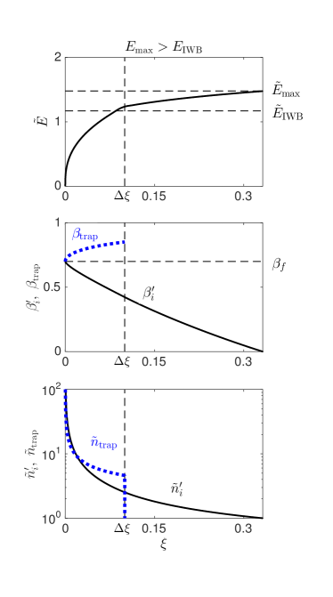
Figure 10: Results of the model of (top panel) the longitudinal electric field $\tilde{E}$, (middle panel) the velocity and (lower panel) density of un-trapped ($\beta_{i}^{\prime}$ and $n_{i}^{\prime}$, black sold lines) and trapped ($\beta_{\rm{trap}}$ and $\tilde{n}_{\rm{trap}}$, thick blue dotted lines) ions when ion trapping just stopped ($\beta_{i}(0)-\beta_{f}\to 0^{-}$ and $\beta_{\rm{trap}}(0)-\beta_{f}\to 0^{+}$). The results are obtained by numerically solving Eqs. (23-27) with $\Delta\xi=0.1$ and the parameters $\beta_{f}$, $n_{e}$, $v_{b}$ the same as those used in Fig. 5. The results are under the condition of $E_{\rm{max}}>E_{\rm{IWB}}$. The upper horizontal dashed line in the top panel marks the maximum electric field $\tilde{E}_{\rm{max}}=1.5$, while the lower one marks $\tilde{E}_{\rm{IWB}}=1.2$. The vertical dashed lines are located at $\xi=\Delta\xi=0.1$.

where $\Delta\xi$ denotes the length of the trapped ion beam. Fig. 10 shows the electric field $\tilde{E}$, the ion velocity ($\beta_{i}^{\prime}$ and $\beta_{\rm{trap}}$) and density ($\tilde{n}_{i}^{\prime}$ and $\tilde{n}_{\rm{trap}}$) by numerically solving Eqs. (23-27). Due to the trapped charge, the electric field in the region $0\leq\xi\leq\Delta\xi$ is significantly increased in comparison to that in Fig. 5 (b). The increase in the electric field eventually closes the gap between the maximum field $E_{\rm{max}}$ driven by the laser pulse and the intrinsic wave breaking field $E_{\rm{IWB}}$.

According to Eqs. (23,24,25), the analogue to Eq. (18) now reads

$$\frac{d}{d\xi}\left(\frac{\tilde{E}^{2}}{2}+\beta_{f}\gamma_{i}^{\prime}\beta_{i}^{\prime}+\tilde{n}_{e}\gamma_{i}^{\prime}(1-\beta_{f}\beta_{i}^{\prime})\right)=\beta_{f}\tilde{E}\tilde{n}_{\rm{trap}}.$$ (28)

Since ion trapping is finished, there is no further self-injection of ions, i.e., the maximum velocity of the untrapped ions must be smaller than or equal to the laser front velocity ($\beta_{i}^{\prime}(0)\leq\beta_{f}$). Integrating Eq. (28) from $\xi=0$ to $\xi=\xi_{b}$, and making use of Eq. (20), we get

$$\beta_{f}\int_{0}^{\xi_{b}}\tilde{n}_{\rm{trap}}(\xi)\tilde{E}d\xi\geq\tilde{E}_{\rm{IWB}}^{2}\chi/2,$$ (29)

where

$$\chi=E_{\rm{max}}^{2}/E_{\rm{IWB}}^{2}-1$$ (30)

characterizes the strength of ion wave breaking. Relation (29) is the condition of no ion injection. It is a generalization of the condition of no ion trapping $\tilde{E}_{\rm{max}}\leq\tilde{E}_{\rm{IWB}}$. When ion trapping just self-stopped, the amount of the trapped ions is the minimum to make relation (29) valid, thus the equal sign has to be taken,

$$\beta_{f}\int_{0}^{\Delta\xi}\tilde{n}_{\rm{trap}}(\xi)\tilde{E}d\xi=\tilde{E}_{\rm{IWB}}^{2}\chi/2.$$ (31)

Equation (31) connects the trapped ions with the laser-driven maximum electric field.

III Ion trapping in 3D geometry

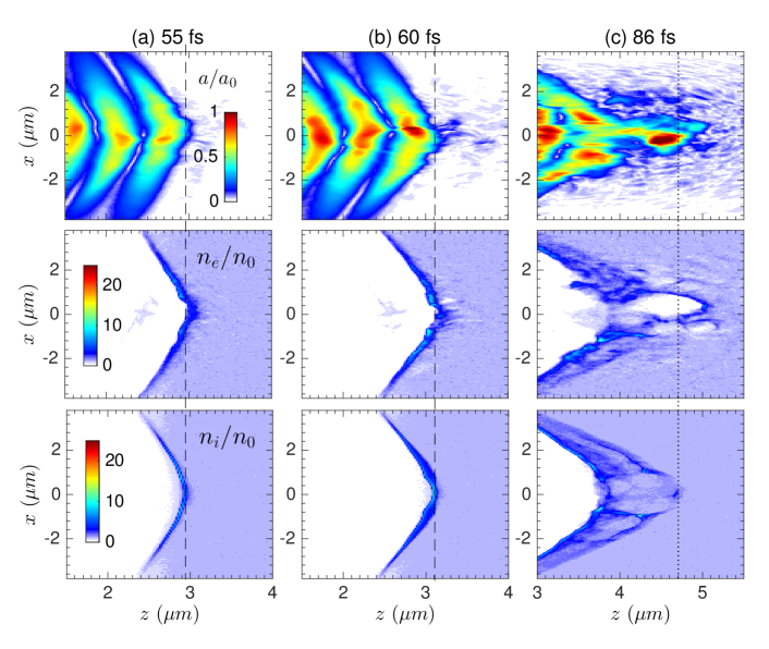
Figure 12: 3D-PIC simulation results shown as cuts in $zx$-plane at $y=0$. From top to bottom, distributions of laser amplitude $a/a_{0}$, electron density $n_{e}/n_{0}$, and ion density $n_{i}/n_{0}$. Column (a) refers to the onset of ion trapping at 55 fs. Column (b) shows the results at 60 fs. The dashed vertical lines in the columns (a) and (b) mark the ion wave breaking points. Column (c) shows the results at 86 fs, when trapping already stops and the trapped ion bunch marked by the dotted vertical line is still accelerating. The initial profiles of laser intensity and plasma density are shown in Fig. 11.

In practical 3D geometry, complexity arises due to transverse effects such as laser self-focusing and electron evacuation. However, ion trapping is essentially an 1D wave breaking process. It occurs localized close to the laser axis (see 3D simulations in Ref. iwba and Fig. 12), especially when the strength of ion wave breaking is small ($\chi\ll 1$). This is different from electron trapping in the bubble regime, where electrons are injected sideways and it is qualitatively different from that in 1D bubble1d3d . We assume footnote4 that the laser spot size is large enough so that in its focus both charge-separation field and ion flow are mainly along the longitudinal direction ($\nabla\cdot\boldsymbol{E}\sim\partial E_{z}/\partial z$ and $\nabla\cdot(n_{i}\boldsymbol{v}_{i})\sim\partial n_{i}v_{i}/\partial z$). Then the 1D model is still capable of describing trapping and acceleration of ions. The difference here is that electrons are expelled transversely by the laser pulse such that $n_{el}\ll n_{i}$. This makes the ion trapping problem solvable.

We consider the condition that ion trapping just stopped so that $\tilde{n}_{i}^{\prime}$ is still singular at $\xi=0$. This allows us to try the power-law ansatz in the range of $0\leq\xi\leq\Delta$,

$$\tilde{n}_{i}^{\prime}(\xi)=\Lambda\xi^{-\Theta},$$ (32)

with $\Lambda>0$ and $\Theta>0$. Then according to Eq. (24) and $\beta_{i}^{\prime}(\xi)\leq\beta_{f}$, we have

$$1-\beta_{i}^{\prime}(\xi)/\beta_{f}=\Lambda^{-1}\xi^{\Theta}.$$ (33)

Applying it to Eq. (23), and making use of the identity $d(\beta\gamma)=\gamma^{3}d\beta$, we find

$$\tilde{E}(\xi)=\beta_{f}\Theta\Lambda^{-2}\xi^{2\Theta-1}\gamma_{i}^{\prime 3}.$$ (34)

The Taylor series of $\gamma_{i}^{\prime}$ at $\beta_{i}^{\prime}=\beta_{f}$ is

$$\gamma_{i}^{\prime}=\gamma_{f}+\gamma_{f}^{3}\beta_{f}(\beta_{i}^{\prime}-\beta_{f})+....$$ (35)

For simplicity we take the first-order approximation, which works very well when

$$\gamma_{f}^{3}\beta_{f}(\beta_{f}-\beta_{i}^{\prime})\ll\gamma_{f}.$$ (36)

Hence, we have

$$\tilde{E}(\xi)=\beta_{f}\gamma_{f}^{3}\Theta\Lambda^{-2}\xi^{2\Theta-1}.$$ (37)

Similarly, when

$$\gamma_{f}^{3}\beta_{f}(\beta_{\rm{trap}}-\beta_{f})\ll\gamma_{f},$$ (38)

we obtain the velocity of the trapped ions by taking Eq. (37) into Eq. (26),

$$\beta_{\rm{trap}}(\xi)/\beta_{f}-1=\Lambda^{-1}\xi^{\Theta}.$$ (39)

Thus, according to Eq. (27), we have

$$\tilde{n}_{\rm{trap}}(\xi)=\Lambda\xi^{-\Theta}.$$ (40)

Then Eq. (25) becomes

$$-\frac{\gamma_{f}^{3}\beta_{f}\Theta}{\xi^{1-\Theta}\Lambda}=-\frac{\beta_{f}\xi^{1-2\Theta}\Lambda^{2}}{(1-\Theta)},$$ (41)

where the electron density has been ignored since $\tilde{n}_{el}\ll\tilde{n}_{i}$ in 3D geometry. Comparing the exponents of $\xi$ and front coefficients on both sides, we get

$$\Theta=2/3,\quad\Lambda=3^{-2/3}\gamma_{f}.$$ (42)

Finally, we have

$$\tilde{E}(\xi) = 2\beta_{f}\gamma_{f}(3\xi)^{1/3},$$ (43)

$$(\beta_{\rm{trap}}(\xi)/\beta_{f}-1)=(1-\beta_{i}^{\prime}(\xi)/\beta_{f}) = \gamma_{f}^{-1}(3\xi)^{2/3},$$ (44)

$$\tilde{n}_{\rm{trap}}(\xi)=\tilde{n}_{i}^{\prime}(\xi) = \gamma_{f}(3\xi)^{-2/3},$$ (45)

and the total ion density

$$\tilde{n}_{i}(\xi)=\tilde{n}_{\rm{trap}}(\xi)+\tilde{n}_{i}^{\prime}(\xi)=2\gamma_{f}(3\xi)^{-2/3}.$$ (46)

By taking Eq. (45) into Eqs. (36) and (38), we find that the scaling approximation (Eqs. (43-46)) is valid under the condition of

$$\xi\ll\frac{1}{3\gamma_{f}^{3/2}\beta_{f}^{3}}.$$ (47)

The scaling result of $\tilde{n}_{\rm{trap}}$ in Eq. (45) helps us to calculate the length of the trapped ion beam according to Eq. (31),

$$\Delta\xi=\frac{1}{3}\left(\frac{\chi}{2}\right)^{3/2}\left(\frac{\tilde{E}_{\rm{IWB}}}{\gamma_{f}\beta_{f}}\right)^{3},$$ (48)

and reduce the areal density of the trapped beam,

$$\tilde{\mathcal{N}}_{\rm{trap}}=\int_{0}^{\Delta\xi}\tilde{n}_{\rm{trap}}(\xi)d\xi=(3\Delta\xi)^{1/3}\gamma_{f}.$$ (49)

Then, in dimensional units with $\mathcal{N}_{\rm{trap}}=(n_{0}v_{f}/\omega_{i})\tilde{\mathcal{N}}_{\rm{trap}}$, we get

$$q_{i}\mathcal{N}_{\rm{trap}}=\frac{q_{i}}{e}\epsilon_{0}E_{\rm{IWB}}\left(\frac{\chi}{2}\right)^{1/2}.$$ (50)

Equation (50) is the central result of the present work. It gives the trapped charge per area $q_{i}\mathcal{N}_{\rm{trap}}$ in terms of the charge number $q_{i}/e$, the displacement $\epsilon_{0}E_{\rm{IWB}}$, corresponding to the threshold electric field for ion wave breaking, and a factor dependent on the strength of ion wave breaking $\chi$.

Both $E_{\rm{max}}$ and $E_{\rm{IWB}}$ depend on the laser amplitude $a_{0}$ and the plasma density $n_{0}$. For fixed $a_{0}$, the threshold for ion wave breaking is defined by $E_{\rm{max}}(n_{0}^{\ast})=E_{\rm{IWB}}(n_{0}^{\ast})$ and allows to calculate the threshold density $n_{0}^{\ast}$. Here, we mark all quantities taken at the wave breaking threshold by an asterisk. Since $\chi(n_{0}^{\ast})=0$, by expanding $\chi(n_{0})$ around $n_{0}=n_{0}^{\ast}$, we get

$$\chi(n_{0})=f_{0}\left(\frac{n_{0}}{n_{0}^{\ast}}-1\right),$$ (51)

where $f_{0}=n_{0}^{\ast}\partial\chi(n_{0}^{\ast})/\partial n_{0}^{\ast}$. Then by using Eq. (20) we find the number of the trapped ions per area in the form

$$\mathcal{N}_{\rm{trap}}\approx f_{1}\frac{\epsilon_{0}E_{0}^{\ast}}{e}\left(\frac{n_{0}}{n_{0}^{\ast}}-1\right)^{1/2},$$ (52)

with $f_{1}=\beta_{f}^{\ast}\left(f_{0}\gamma_{f}^{\ast}\left(1-\delta^{\ast}\right)\right)^{1/2}$ and $\delta^{\ast}=\beta_{b}^{\ast}\gamma_{b}^{\ast}/\beta_{f}^{\ast}\gamma_{f}^{\ast}$, since $\tilde{n}_{el}=0$. This result holds for fixed laser intensity and densities $n_{0}$ just beyond threshold density $n_{0}^{\ast}$. The precise value of the front factor $f_{1}$ in Eq. (52) depends on the details not considered in the present paper. Comparing with the simulation results in Sec. IV, it turns out to be of order one. We emphasize that the scaling exponent $1/2$ in Eq. (52) traces back to the power-law exponents in Eqs. (43,45).

With the same approach, we also obtain the power-law scalings when ion wave breaking just sets in ($E_{\rm{max}}\to E_{\rm{IWB}}$ and $\tilde{n}_{\rm{trap}}=0$),

$$\tilde{E}(\xi) = 2^{1/3}\beta_{f}\gamma_{f}(3\xi)^{1/3},$$ (53)

$$(1-\beta_{i}(\xi)/\beta_{f}) = 2^{-1/3}\gamma_{f}^{-1}(3\xi)^{2/3},$$ (54)

$$\tilde{n}_{i}(\xi) = 2^{1/3}\gamma_{f}(3\xi)^{-2/3}.$$ (55)

One observes that the power-law exponents are the same as those in Eqs. (43,44,45), but the coefficients are different. The change of the coefficients is a signal of ion trapping.

IV 3D PIC simulations

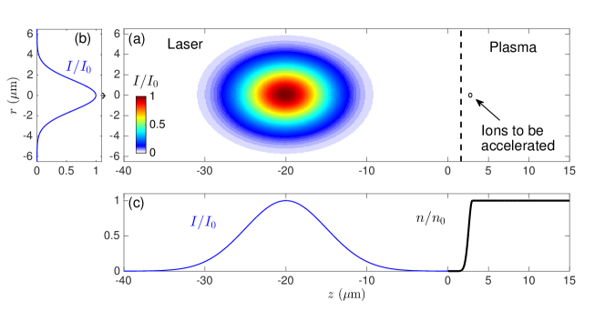
Figure 11: (a) Initial distributions of the laser intensity and the target. The laser pulse is circularly polarized with laser wave length $1\mu m$ and Gaussian intensity distribution in both (b) radial ($r$) and (c) longitudinal ($z$) directions. The intensity is $I=I_{0}\exp(-2r^{2}/R_{L}^{2})\exp(-2(z-z_{a})^{2}/(c\tau_{L})^{2})$, where $I_{0}=6\times 10^{20}\rm{W/cm^{2}}$, $R_{L}=3\mu m$, $z_{a}=-20\mu m$, and $\tau_{L}=33.3$ fs. The plasma target consists of protons and electrons with plasma density $n_{0}=8\times 10^{21}{\rm{cm}}^{-3}$ uniformly distributed in the range of $z>3\mu m$ and a Gaussian profile density ramp $n=n_{0}\exp(-(z-z_{n})^{2}/\sigma_{n}^{2})$ for $z<3\mu m$, where $z_{n}=3\mu m$ and $\sigma_{n}=0.63\mu m$. Ions to be accelerated are initially in a small volume ($2.7um<z<3um$ and $r<0.2um$, see Fig. 14 and the corresponding text), as marked by the small black circle and the black arrow in (a).

We have carried out 3D PIC simulations to verify the model predictions, using the plasma simulation code (PSC) psc . A circularly polarized laser pulse with wavelength $\lambda_{L}=1\rm{\mu m}$ is vertically incident on hydrogen plasma ($m_{i}/m_{e}=1836$ and $q_{i}/e=1$) with bulk density $n_{0}=7.2n_{c}$. At the surface, the density rises in the region $0<z<z_{n}$ according to $n(z)=n_{0}\exp(-(z-z_{n})^{2}/\sigma_{n}^{2})$ with $z_{n}=3\rm{\mu m}$ and $\sigma_{n}=0.63\rm{\mu m}$. Such a slow rising boundary is reasonable in describing a target that is pre-heated by a laser pre-pulse. We have also run simulations with different $\sigma_{n}$ and found that results are insensitive to $\sigma_{n}$ for $0\leq\sigma_{n}\leq 1\mu m$. The peak laser intensity is $I_{0}=6\times 10^{20}\rm{W/cm^{2}}$, corresponding to a laser amplitude $a_{0}=15$. We have chosen a relatively low value of intensity to demonstrate that ion trapping by ion wave breaking can already be studied with laser pulses presently available experimentally. Also, the shape of the pulse incident from the left side ($z=0$) is modelled by a Gaussian amplitude in both radial direction $\left(r=\sqrt{x^{2}+y^{2}}\right)$ and time, $a(r,t)=a_{0}\exp(-r^{2}/R_{L}^{2})\exp(-(t-t_{0})^{2}/\tau_{L}^{2})$ with $\tau_{L}=33.33$ fs (10 laser cycles), $R_{L}=3\rm{\mu m}$, and $t_{0}=66.67$ fs, implying a moderate contrast ratio at the pulse front. The initial distributions of laser intensity and plasma density are shown in Fig. 11. In order to resolve the details of the ion motion, in particular near the wave breaking point, we have used 50 cells per micron and 10 macro-particles per cell for each species. The initial temperatures are set to 10 keV for electrons and 1 keV for ions.

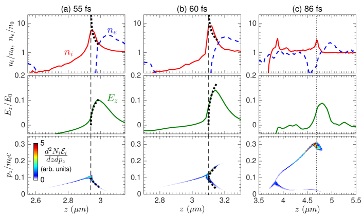
Figure 13: Comparison of on-axis ion evolution from the simulation in Fig. 12 with our model (black dotted curves in the first two columns) near the point of ion wave breaking, showing (top panels) ion density $n_{i}/n_{0}$ (red solid lines), electron density $n_{e}/n_{0}$ (blue dashed lines), (middle panels) longitudinal electric field $E_{z}/E_{0}$ (green solid lines), and (lower panels) ion kinetic energy density ($d^{2}N_{i}\mathcal{E}_{i}/dzdp_{z}$ in arbitrary units) in phase space $(z,p_{z}/m_{i}c)$. The simulation results are obtained by taking average over $r\leq 0.2\rm{\mu m}$. The dashed vertical lines in columns (a) and (b) mark the ion wave breaking points. The dotted vertical line in column (c) marks the position of the trapped ion bunch.

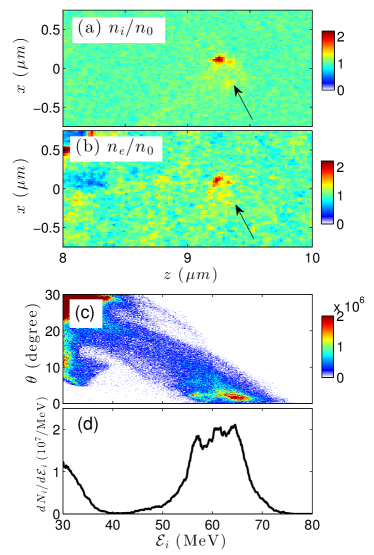
Figure 14: Results of the output ion beam at 130 fs for the simulation in Fig. 12. Distributions of (a) ion density and (b) electron density as cuts in $zx$-plane at $y=0$. (c) Ion angular-energy ($\theta$-$\mathcal{E}_{i}$) distribution ($d^{2}N_{i}/d\theta d\mathcal{E}_{i}$ in arbitrary units) and (d) ion energy spectrum ($dN_{i}/d\mathcal{E}_{i}$) for ions within $\theta<10$ degrees. The ion beam and the corresponding electron beam in (a) and (b) are marked by black arrows, respectively. Most of the accelerated ions initially come from the small region marked by a black arrow in Fig. 11 (a).

The simulation results are shown in Figs. 12 and 13 as snapshots at different times. Figure 12 shows the distributions of laser field, electron density, and ion density in $zx$-plane, while Fig. 13 shows the density of electrons and ions, the longitudinal electric field, and the ion phase space ($p_{z}/m_{i}c,z$) averaged over $r\leq 0.2~{}\rm{\mu m}$ along the laser axis. At 55 fs (column (a)), the front rising part of the laser pulse with relatively low-intensity has been depleted (Fig. 12 (a) top panel), and the laser front propagates forward with a relatively stable velocity $v_{f}\sim 0.1c$. It varies slowly until $t\sim 65fs$. The ion wave develops a sharp peak in density at $z\approx 2.94~{}\rm{\mu m}$ and is about to break. The maximum ion velocity is almost equal to the laser front velocity (Fig. 13 (a) bottom panel). The local distributions near the ion wave peak match well with the power-law scalings given by Eqs. (53,54,55) (dotted black lines in Fig. 13 (a)). The charge-separation field increases with time. The strongest charge-separation field is observed at 60 fs (column (b)), with the field maximum $E_{\rm{max}}\sim 0.14E_{0}$. Ion trapping is now in progress. A good portion of the ions has already been trapped and is accelerating in the region $z>3.1~{}\rm{\mu m}$. Ion density and electric field have increased in agreement with the results of our model, now given by Eqs. (43,44,45). With the interaction time increasing the laser self-focusing effect becomes important. It leads to an increase of laser intensity on axis and enhances the acceleration of the trapped ions. Later at 86 fs (column (c)), the focused laser pulse penetrates into the plasma and expels electrons, producing a cavity with relatively low electron density (Fig. 12 (c) middle panel). Ions dragged by the expelled electrons form a high density shell (Fig. 12 (c) bottom panel). An ion bunch is observed at the point $r\simeq 0$ and $z\simeq 4.7\rm{\mu m}$, both in Fig. 12 (c) bottom panel and Fig. 13 (c) top and bottom panels. The bunch propagates to the right with speed $\approx 0.3c$, faster than the laser front velocity, which now is $v_{f}\sim 0.2c$ due to the laser self-focusing. This corresponds to a proton energy of $(40\pm 10)$ MeV at this time. The ion beam will further gain energy (reaching about 65 MeV, see Fig. 14 (d)), before overtaking the laser front and then freely cruising to the right.

Since the trapped ion beam is localized close to the laser axis and mainly accelerated forward, its areal density almost keeps constant during the acceleration process. At 86 fs, the trapped ion beam is already distinguished from background ions in both real space and phase space. As is seen in Fig. 12 (c) bottom panel and Fig. 13 (c) top and bottom panels, the length of the ion beam is $\sim 0.2\mu m$, and the peak density is $\sim 8n_{c}$, corresponding to the ion number per area $e\mathcal{N}_{\rm{trap}}\sim 0.08\epsilon_{0}E_{0}$. This can be explained by the wave breaking model. According to the observations in Fig. 13 (b,c,e,f), we have $v_{b}\sim v_{f}/2\sim 0.05c$ (for example, in Fig. 13 (a), we chose $v_{b}$ as the ion velocity at the point $z=3\mu m$ where $E_{z}$ peaks). By taking the parameters $a_{0}\sim 15$ and $n_{0}\sim 7.2n_{c}$, and using Eq. (20), we get $E_{\rm{IWB}}=0.1E_{0}$. Then according to Eq. (50) and making use of $E_{\rm{max}}\sim 0.14E_{0}$ we have $e\mathcal{N}_{\rm{trap}}=0.07\epsilon_{0}E_{0}$, close to the result directly observed in the simulation.

Ion acceleration stops when the trapped ion beam overtakes the laser front. After that, the output ion beam moves in the plasma freely, accompanied by an almost equivalent electron beam, as shown in Fig. 14 (a,b). The neutralized beam can propagate in plasma for a very long distance almost without energy loss. Furthermore, the ion beam is very compact. It is distributed in a small space volume ($\sim 0.2\mu m^{3}$) with the peak density $\sim 8n_{c}$. It contains about $2.6\times 10^{8}$ ions. The divergence angle is less than 5 degrees (Fig. 14 (c)). The corresponding energy spectrum is quasi-mono-energetic and peaks at about 65 MeV with an energy spread of about 10 MeV (Fig. 14 (d)). By tracking ions in the simulation we find that most of the ions in the output ion beam initially come from a small spherical-like region ($2.7um<z<3um$ and $r<0.2um$) marked by a black arrow in Fig. 11 (a). This confirms that ion trapping mainly happens in the time period between 55 fs and 60 fs.

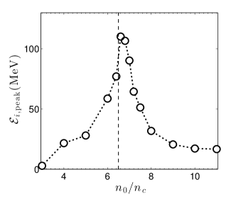
Figure 15: 3D PIC simulation results of Peak ion energy $\mathcal{E}_{i,\rm{peak}}$ (black circles), with the same laser pulse as that shown in Fig. 11, but different initial plasma densities $n_{0}/n_{c}$. The dashed vertical line at $n_{0}/n_{c}=6.5$ marks the threshold density for ion trapping and acceleration.

Simulation results of peak ion energy $\mathcal{E}_{i,\rm{peak}}$ for different initial plasma densities $n_{0}$ are shown in Fig. 15. The most energetic ion acceleration occurs for initial plasma density $n_{0}=6.6n_{c}$, with peak energy about 110 MeV. For $n_{0}\leq 6.4n_{c}$ there is no output ion beam on the laser axis and the final ion spectra have no clear peaks (the maximum ion energies are plotted instead). The threshold density for ion wave breaking is then obtained approximately as $n_{0}^{\ast}\sim 6.5n_{c}$, marked by a vertical dashed line in Fig. 15. Beyond it, the peak ion energies decrease with the increase of the initial plasma density. For $n_{0}>8.5n_{c}$ the plasma becomes opaque and our model does not apply.

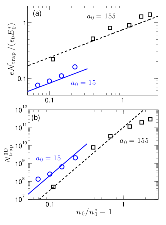
Figure 16: (a) The number of trapped ions per area $\mathcal{N}_{\rm{trap}}$ and (b) the total number of the accelerated ions $N_{\rm{trap}}^{\rm{3D}}$ for fixed laser amplitude $a_{0}$ versus $(n_{0}/n_{0}^{\ast}-1)$, where $n_{0}$ denotes the initial target density and $n_{0}^{\ast}$ the threshold density for ion trapping. Circles and squares refer to 3D PIC simulations and the lines in (a) to Eq. (52) and in (b) to Eq. (56); blue circles (case 1, $a_{0}=15$, $n_{0}^{\ast}=6.5n_{c}$) corresponding to the 3D simulations shown in Fig. 15 and black sqares (case 2, $a_{0}=155$, $n_{0}^{\ast}=1.8n_{c}$) to 3D simulations reported in Ref. iwba .

In Fig. 16 (a), we compare values of $\mathcal{N}_{\rm{trap}}$ from simulations with those from Eq. (52) for laser pulses having very different amplitudes: Case 1 with $a_{0}=15$ (blue, Gaussian distributions in both space and time, shown in Fig. 11) and case 2 with $a_{0}=155$ (black, Gaussian distribution in space and super-Gaussian in time, reported in Ref. iwba ). They correspond to threshold densities $n_{0}^{\ast}\simeq 6.5n_{c}$ for case 1 and $n_{0}^{\ast}\simeq 1.8n_{c}$ (peak ion energy about 6 GeV) for case 2. The simulation results are well described by the square root scaling, represented by the straight lines with slope 1/2 in the double-logarithmic plot. The position of these lines has been adjusted by choosing $f_{1}=0.25$ for case 1 and $f_{1}=0.75$ for case 2 in Eq. (52). It demonstrates that the present scaling result holds over laser intensities ranging from $10^{20}$ to $10^{22}$W/cm².

The 3D PIC simulations provide us with absolute numbers of accelerated ions; they are plotted in Fig. 16 (b). In simulations we have found that for a given laser pulse the trapped ion beams appear as bullet-like bunches with transverse sizes $\Delta r$ scale roughly linearly with the longitudinal ones $\Delta z$, especially when $\chi\ll 1$. The longitudinal size is estimated as $\Delta z=(c\beta_{f}^{\ast}/\omega_{i}^{\ast})\Delta\xi$, where $\Delta\xi=\left(f_{0}\left(1-\delta^{\ast}\right)\left(n_{0}/n_{0}^{\ast}-1\right)/\gamma_{f}^{\ast}\right)^{3/2}/3$, obtained by applying Eqs. (20) and (51) to Eq. (48). Therefore, we estimate the absolute number of trapped and accelerated ions as

$$N_{\rm{trap}}^{\rm{3D}}\approx(\Delta r)^{2}\mathcal{N}_{\rm{trap}}\approx f_{2}\left(\frac{c}{\omega_{i}^{\ast}}\right)^{2}\frac{\epsilon_{0}E_{0}^{\ast}}{e}\left(\frac{n_{0}}{n_{0}^{\ast}}-1\right)^{7/2}.$$ (56)

The straight lines in Fig. 16 (b) with slope 7/2 appear to describe the behaviour of the simulation points quite well. Here we have used adjustment factors $f_{2}=2$ for case 1 and $f_{2}=0.4$ for case 2.

V Conclusions

In summary, we have investigated ion trapping and acceleration near the threshold where ion trapping initiates. The dynamics of self-regulating ion trapping has been identified as a process of essentially one-dimensional ion wave breaking. We have succeeded to determine the power-law profiles of the ion flow at the instant of wave breaking and the finite amount of charge that is trapped and accelerated. The threshold electric field for ion wave breaking, $E_{\rm{IWB}}$, has been found to be a function of laser front velocity. The trapped ion charge depends on the strength of ion wave breaking, which is characterized by how much the maximum of the charge-separation field $E_{\rm{max}}$ driven by the laser pulse exceeds $E_{\rm{IWB}}$. This can be controlled by tuning laser intensity and plasma density. Near the threshold this charge is small and localized such that high-quality ion bunches with low energy spread and beam emittance are expected. We hope that the present results stimulate experiments to explore this regime, which occurs in relativistically transparent plasma just below the regime of hole boring.

References

- (1) H. Daido, M. Nishiuchi, and A. S. Pirozhkov, Rep Prog Phys 75, 056401 (2012); A. Macchi, M. Borghesi, and M. Passoni, Rev. Mod. Phys. 85, 751 (2013); M. Borghesi, Nucl. Instr. Meth. A740, 6 (2014); J. Schreiber, P. R. Bolton, and K. Parodi, Rev. Sci. Instrum. 87, 071101 (2016).
- (2) S.V. Bulanov and V.S. Khoroshkov, Plasma Phys. Rep. 28, 453 (2002); V. Malka, J. Faure, Y. A. Gauduel, E. Lefebvre, A. Rousse, and K. T. Phuoc, Nature Physics 4, 447 (2008); D. Schardt, T. Elsässer, and D. Schulz-Ertner, Rev. Mod. Phys. 82, 383 (2010);
- (3) P. Patel, A. Mackinnon, M. Key, T. Cowan, M. Foord, M. Allen, D. Price, H. Ruhl, P. Springer, and R. Stephens, Phys. Rev. Lett. 91, 125004 (2003);
- (4) M. Roth, T.E. Cowan, M.H. Key, S.P. Hatchett, C. Brown, W. Fountain, J. Johnson, D.M. Pennington, R.A. Snavely, S.C. Wilks, K. Yasuike, H. Ruhl, F. Pegoraro, S.V. Bulanov, E.M. Campbell, M.D. Perry, and H. Powell, Phys. Rev. Lett. 86, 436 (2001);
- (5) S. C. Wilks, W. L. Kruer, M. Tabak, and A. B. Langdon, Phys. Rev. Lett. 69, 1383 (1992); A. Macchi, F. Cattani, T.V. Liseykina, and F. Cornolti, Phys. Rev. Lett. 94, 165003 (2005).
- (6) A. P. L. Robinson, M. Zepf, S. Kar, R. G. Evans, and C. Bellei, New J. Phys. 10, 013021 (2008); O. Klimo, J. Psikal, J. Limpouch, and V. T. Tikhonchuk, Phys. Rev. ST Accel. Beams 11, 117 (2008); X. Q. Yan, C. Lin, Z. M. Sheng, Z. Y. Guo, B. C. Liu, Y. R. Lu, J. X. Fang, and J. E. Chen, Phys. Rev. Lett. 100, 135003 (2008); B. Qiao, M. Zepf, M. Borghesi, and M. Geissler, Phys. Rev. Lett. 102, 145002 (2009); A. Macchi, S. Veghini, and F. Pegoraro, Phys. Rev. Lett. 103, 085003 (2009); A. Macchi, S. Veghini, T. V. Liseykina, and F. Pegoraro, New J. Phys. 12, 045013 (2010).
- (7) T. Esirkepov, M. Borghesi, S. V. Bulanov, G. Mourou, and T. Tajima, Phys. Rev. Lett. 92, 175003 (2004); N. Naumova, T. Schlegel, V. T. Tikhonchuk, C. Labaune, I. V. Sokolov, and G. Mourou, Phys. Rev. Lett. 102, 25002 (2009); T. Schlegel, N. Naumova, V. T. Tikhonchuk, C. Labaune, I. V. Sokolov, and G. Mourou, Physics of Plasmas 16, 083103 (2009).
- (8) A. P. L. Robinson, Physics of Plasmas 18, 056701 (2011).
- (9) S. M. Weng, M. Murakami, P. Mulser, and Z. M. Sheng, New J. Phys. 14, 063026 (2012).
- (10) A. A. Sahai, F. S. Tsung, A. R. Tableman, W. B. Mori, and T. C. Katsouleas, Phys. Rev. E 88, 043105 (2013).
- (11) A. V. Brantov, E. A. Govras, V. F. Kovalev, and V. Y. Bychenkov, Phys. Rev. Lett. 116, 085004 (2016).
- (12) A. V. Brantov, P. A. Ksenofontov, and V. Y. Bychenkov, Physics of Plasmas 24, 113102 (2017).
- (13) B. Liu, J. Meyer-ter-Vehn, K.-U. Bamberg, W. J. Ma, J. Liu, X. T. He, X. Q. Yan, and H. Ruhl, Phys. Rev. Accel. Beams 19, 073401 (2016).
- (14) W. Ma, L. Song, R. Yang, T. Zhang, Y. Zhao, L. Sun, Y. Ren, D. Liu, L. Liu, J. Shen, Z. Zhang, Y. Xiang, W. Zhou, and S. Xie, Nano Lett. 7, 2307 (2007).
- (15) L. Willingale, S. R. Nagel, A. G. R. Thomas, C. Bellei, R. J. Clarke, A. E. Dangor, R. Heathcote, M. C. Kaluza, C. Kamperidis, S. Kneip, K. Krushelnick, N. Lopes, S. P. D. Mangles, W. Nazarov, P. M. Nilson, and Z. Najmudin, Phys. Rev. Lett. 102, 125002 (2009).
- (16) Y. Fukuda, A. Y. Faenov, M. Tampo, T. A. Pikuz, T. Nakamura, M. Kando, Y. Hayashi, A. Yogo, H. Sakaki, T. Kameshima, A. S. Pirozhkov, K. Ogura, M. Mori, T. Z. Esirkepov, J. Koga, A. S. Boldarev, V. A. Gasilov, A. I. Magunov, T. Yamauchi, R. Kodama, P. R. Bolton, Y. Kato, T. Tajima, H. Daido, and S. V. Bulanov, Phys. Rev. Lett. 103, 165002 (2009).
- (17) A. V. Brantov, E. A. Obraztsova, A. L. Chuvilin, E. D. Obraztsova, and V. Y. Bychenkov, Phys. Rev. Accel. Beams 20, 061301 (2017).
- (18) P. Kaw, Phys. Fluids 13, 472 (1970).
- (19) O. Shorokhov and A. Pukhov, Laser Part. Beams 22, 175-181 (2004).
- (20) B. Shen, Y. Li, M. Y. Yu, and J. Cary, Phys. Rev. E 76, 055402(R) (2007).
- (21) A. I. Akhiezer and R. V. Polovin, JETP Lett. 3, 696 (1956).
- (22) In Ref. Akhiezer , unmagnetized Maxwell equations are used. In our case, Eqs. (2,4,5) are physically equivalent to the unmagnetized Maxwell equations.
- (23) J. M. Dawson, Phys. Rev. 113, 383 (1959).
- (24) E. Esarey, C. B. Schroeder, and W. P. Leemans, Rev. Mod. Phys. 81, 1229 (2009).
- (25) By combining Eqs. (6,8,10,11,12), two integrals are obtained, and By applying them at the point where , , and , and the point where , , one has , where , and When , one gets , and . Then Eq. (13) is obtained.
- (26) H. Ruhl, Classical particle simulations, in Introduction to Computational Methods in Many Body Physics, edited by M. Bonitz, and D. Semkat (Rinton, Paramus, New Jersey, 2006).
- (27) see, e.g., L. Willingale, S. Nagel, A. Thomas, C. Bellei, R. Clarke, A. Dangor, R. Heathcote, M. Kaluza, C. Kamperidis, S. Kneip, K. Krushelnick, N. Lopes, S. Mangles, W. Nazarov, P. Nilson, and Z. Najmudin, Phys. Rev. Lett. 102, 125002 (2009).
- (28) A. P. L. Robinson, P. Gibbon, M. Zepf, S. Kar, R. G. Evans, and C. Bellei, Plasma Phys. Control. Fusion 51, 024004 (2009).
- (29) see, e.g., A. Macchi, S. Veghini, and F. Pegoraro, Phys. Rev. Lett. 103, 085003 (2009).
- (30) In the hole-boring regime hb , all ions in the laser focus are accelerated, therefore, the condition of relativistic transparency discussed in Ref. trans breaks down, and the plasma becomes opaque.
- (31) In a reflection process one has , where and denote the incoming and reflected current densities in the frame comoving with the laser front, respectively. It is valid in the region where . By using the Lorentz transformation one gets and , where and are current densities in the laboratory frame. Then the equation is obtained.
- (32) I. Kostyukov, A. Pukhov, and S. Kiselev, Physics of Plasmas 11, 5256 (2004); S. Gordienko and A. Pukhov, Physics of Plasmas 12, 043109 (2005).
- (33) The coefficients in Eqs. (43-46) and Eqs. (53-55) may change if this assumption breaks down, however, it is easy to find that the power-law exponents in these equations are still the same.