Improving performance of SEOBNRv3 by $\mathord{\sim}$300x

Abstract

When a gravitational wave is detected by Advanced LIGO/Virgo, sophisticated parameter estimation (PE) pipelines spring into action. These pipelines leverage approximants to generate large numbers of theoretical gravitational waveform predictions to characterize the detected signal. One of the most accurate and physically comprehensive classes of approximants in wide use is the “Spinning Effective One Body–Numerical Relativity” (SEOBNR) family. Waveform generation with these approximants can be computationally expensive, which has limited their usefulness in multiple data analysis contexts. In prior work we improved the performance of the aligned-spin approximant SEOBNR version 2 (v2) by nearly 300x. In this work we focus on optimizing the full eight-dimensional, precessing approximant SEOBNR version 3 (v3). While several v2 optimizations were implemented during its development, v3 is far too slow for use in state-of-the-art source characterization efforts for long-inspiral detections. Completion of a PE run after such a detection could take centuries to complete using v3. Here we develop and implement a host of optimizations for v3, calling the optimized approximant v3_Opt. Our optimized approximant is about 340x faster than v3, and generates waveforms that are numerically indistinguishable.

1 Introduction

With its first detections of gravitational waves [1, 2, 3, 4, 5, 6], the Advanced Laser Interferometer Gravitational Wave Observatory (Advanced LIGO) has provided a fundamentally new means of observing the Universe. At the heart of each of these detections was a merger of compact binaries. In such binaries, each compact object possesses four intrinsic parameters: mass, and the three components of the spin vector. Inferring all eight intrinsic parameters from a gravitational wave observation, which analysis is part of the more general parameter estimation (PE), remains a challenging and computationally expensive enterprise.

The LIGO/Virgo Scientific Collaboration (LVC) performs PE in a Bayesian framework, implemented within the lalinference software package that is part of the larger open-source software framework LALSuite [7]. In such a framework, we sample the posterior distribution by repeatedly calculating the likelihood that a particular waveform matches the data and applying Bayes’ theorem. Evaluating the likelihood requires the rapid, sequential generation of as many as $\mathord{\sim}10^{8}$ theoretical gravitational wave predictions [8]. Generating so many predictions via a full solution of the general relativistic field equations (using the tools of numerical relativity) would be far too computationally expensive. Thus theoretical models adopted for PE generally employ approximate solutions called approximants. State-of-the-art approximants adopt post-Newtonian techniques for evaluating the gravitational waveform throughout most of the inspiral and ringdown, and inject information from numerical relativity calculations for the late inspiral and merger.

One such gravitational wave approximant is the Spinning Effective One Body–Numerical Relativity (SEOBNR) algorithm. This algorithm marries an effective-one body inspiral gravitational waveform approximation—with unknown higher-order terms fit to numerical relativity-generated gravitational wave predictions—to a black hole ringdown model [9]. In particular, SEOBNR starts with the Effective One Body (EOB) approach to non-spinning binary modeling [10] by mapping the dynamics of the two-body system to the dynamics of an effective particle moving in a deformed Schwarzschild metric. This work was then extended to include the effects of spinning, precessing binaries [11]. Implemented numerically, this Spinning EOB procedure adopts a precessing source frame in which precession-induced variations in amplitude and phase are minimized during inspiral, and a source frame aligned with the spin of the final body for matching the inspiral to the merger-ringdown [9].

The other widely adopted approximant within the LVC for PE is the Phenom series of phenomenological waveform models. These waveform models are based on the combination of accurate post-Newtonian inspiral models with late-inspiral and merger phenomenological fits to suites of numerical relativity simulations [12]. More recently, Phenom models have been built to include the effects of precession [13]. In particular, precession effects are included by using post-Newtonian methods to compute precession angles and then “twisting” the underlying non-precessing model [13, 14, 15]. Phenom models are simulated completely in the frequency domain, and therefore simplify some aspects of analysis. The only Phenom model designed to generate gravitational waveform predictions across all eight dimensions of parameter space is PhenomP [13], which was extensively used in the first six detection papers. We remark that Phenom is limited to a relatively small number of numerical relativity simulations against which it has been calibrated, and it is difficult to determine the degree of systematic uncertainty in the model without appealing to another model for comparison.

Evaluating the systematic uncertainties of the Phenom model requires construction of an independent gravitational waveform model with independent systematics, and the SEOBNR family of models is a good candidate for this task. The only SEOBNR model capable of generating theoretical gravitational waveform predictions in all 8 intrinsic dimensions of parameter space is the third version of the model, v3; the first and second versions were restricted to aligned-spin cases. In particular, v3 was built to accommodate arbitrary mass ratios, spin magnitudes, and spin orientations and has been calibrated and validated against a variety of numerical relativity simulations [16]. Thus v3 is vital for precessing compact binary merger PE.

Unfortunately, v3 is too currently too slow for PE. A single waveform generation across the LIGO band for, say, a black hole-neutron star system using v3 can take as long as an hour on a modern desktop computer. If LIGO observed a black hole-neutron star system merge, a sequential-gravitational-wave-generation PE would take thousands of years. Attempts to overcome the computational challenge of generating such time-consuming gravitational waveforms include the construction of Reduced Order Model (ROM) approximants. ROMs make use of multidimensional interpolations between sampled points in another underlying approximant. For example, a ROM based on the aligned-spin SEOBNR version 2 (v2) approximant [17, 18] is constructed by first generating an extensive collection of waveform predictions using v2 that adequately samples the 4D parameter space reliably covered by v2. Then to obtain the gravitational waveform at any desired point in parameter space, the ROM simply interpolates within the four dimensions of sampled parameter space. A ROM version of v2 can generate waveforms up to $\mathord{\sim}3000$x faster than v2 directly [17], which explains in part why ROMs enjoy such widespread use within the LVC for data analysis applications.

While ROMs have been constructed with favorable performance characteristics in aligned-spin situations, the cost of generating a ROM grows exponentially with the dimension of the ROM (though see [19] for ideas on combating this using a reduced basis approach). No strategy yet exists that can perform the 8-dimensional (8D) interpolations faster than the 8D approximant; until such a strategy is invented, the most promising way to improve the performance of theoretical waveform generation in the full 8D parameter space will be to optimize the approximant directly. As a proof-of-principle, we demonstrated that such an approach is capable of improving the performance of the aligned-spin v2 approximant by a typical factor of $\mathord{\sim}280$x [20]. We call our optimized v2 approximant v2_opt. The precessing (8D) v3 approximant was in development as we independently prepared v2_opt, and thus originally contained all the same inefficiencies as v2. This suggests that if the full suite of optimizations we implemented in v2 were incorporated into v3, v3-based PE timescales might drop by two orders of magnitude at least.

This paper documents our incorporation of applicable v2 optimizations into v3, as well as our implementation of innovative new optimization ideas, which together act to speed up v3 by $\mathord{\sim}340$x. Optimization strategies are summarized in Sec. 2. Section 3 presents code validation tests that demonstrate roundoff-level agreement between v3 and our latest optimized version of v3, designated v3_Opt, along with benchmarks providing an overview of performance gains across parameter space in v3_Opt. For convenience, Table 1 defines all SEOBNR approximants referenced in this paper.

Base Approx. Description Approximant Name SEOBNRv2 v2 Initial SEOBNRv2 implementation; see [21]. (spin-aligned) v2_opt Optimized v2footnote 2; see [20]. SEOBNRv3 v3_preopt Initial SEOBNRv3 implementation; see [9]. (precessing) v3 Partially optimized v3_preopt with bug fixes. v3_pert v3 with machine-$\epsilon$ mass perturbation footnote 4. v3_opt v3 optimized similarly to v2_opt footnote 4. v3_Opt v3_opt with new optimization strategies. v3_Opt_rk4 v3_Opt implementing RK4 rather than RK8footnote 5.

Table 1: Approximant naming conventions. These conventions apply throughout this paper.

2 SEOBNRv3_opt: Optimizations migrated from v2_opt

Optimizations to v3 were performed in two phases. In the first phase, described in Sec. 2.1, we migrated to v3 all applicable optimizations developed during the preparation of v2_opt. Sections 2.2 and 2.3 detail the second phase of optimization, outlining new strategies incorporated into v3_Opt.

2.1 Migrated Optimizations

Here we summarize the optimizations to v2 which were migrated to v3 and thus implemented in v3_opt.

• Switching compilers. Switching from the GNU Compiler Collection (gcc) [22] C compiler to the Intel Compiler Suite (icc) [23] C compiler improves performance by roughly a factor of 2x. It is well-known that the icc compiler often produces more efficient executables than the gcc compiler.

• Minimize transcendental function evaluations. The EOB Hamiltonian equations of motion were hand-optimized by minimizing calls to some expensive transcendental functions such as exp(), log(), and pow().

• Replacing finite difference with exact derivatives. When solving the EOB Hamiltonian equations of motion, v3 computes partial derivatives of the Hamiltonian using finite difference approximations. We replaced these with exact, Mathematica-generated expressions for the derivatives, using Mathematica’s code generation facilities—which includes common subexpression elimination (CSE)—to generate the C code [24]. Although this alone acts to significantly speed up v3, in this work we further optimize these Mathematica-generated derivatives.

• Increasing the order of the ODE solver. v3 solves the EOB Hamiltonian equations of motion via a Runge-Kutta fourth order (RK4) ODE solver. After implementing exact derivatives, we noticed that the number of RK4 steps needed dropped significantly—presumably due to the effective removal of high numerical noise intrinsic to finite-difference derivatives. We then found that adopting a Runge-Kutta eighth order (RK8) ODE solver resulted in 2x larger timesteps, so an even larger speed-up was observed.

• Reducing orbital angular velocity calculations. The orbital angular velocity $\omega$ was calculated for each ($\ell,m$) mode (as defined in [9]) inside the ODE solver. As $\omega$ exhibits no dependence on $\ell$ or $m$, this expensive recalculation was unnecessary and needs only be performed once.

For more details about these optimizations see our v2 optimization paper [20].

2.2 Guided Automatic Differentiation: A more efficient way of generating symbolic derivatives of the Hamiltonian

After migrating the v2 optimizations described in Sec. 2.1 to v3, profiling analyses indicated that approximately $75\%$ of v3_opt’s total runtime was spent computing the v3 Hamiltonian [9] and its partial derivatives with respect to the twelve degrees of freedom (consisting of three spatial degrees $\{x,y,z\}$, three momentum degrees $\{p_{x},p_{y},p_{z}\}$, and three spin degrees for each of the two binary components $i\in\{1,2\}$: $\{s_{i}^{x},s_{i}^{y},s_{i}^{z}\}$).

In v3, the ODE solver computes these partial derivatives by direct evaluations of the Hamiltonian itself via finite difference techniques [21]. In v3_opt, these numerical derivatives were replaced with Mathematica-generated exact derivatives. Although these exact derivatives unlock significant performance gains, the Mathematica-generated C code was neither particularly human-readable (comprising thousands of lines of code output by Mathematica’s CSE routines) nor particularly well-optimized (common patterns were still visible and recomputed in the C code). Attempts to gain performance through consolidation of all derivatives—as was possible in our optimizations of v2—proved beyond Mathematica’s capabilities when differentiating the v3 Hamiltonian on our high-performance workstations. Therefore, C codes for all twelve exact derivatives needed to be output separately, resulting in a significant number of unnecessary re-computations.

We present here our new strategy for computing partial derivatives of the Hamiltonian, called guided automatic differentiation (GAD), which results in a significant reduction in computational cost while ensuring the resulting code is highly human-readable. GAD is based on forward accumulation automatic differentiation, with the advantage of the subexpressions being chosen by hand to minimize the overall number of floating point operations.

The following describes the process of computing a partial derivative of the v3 Hamiltonian $H$ with respect to an arbitrary independent variable $x_{1}$ using GAD. We may write $H$ in the following form, where $I$ is a set of input quantities:

$$v_{1} =f_{1}(I)$$

$$v_{2} =f_{2}(v_{1},I)$$

$$v_{3} =f_{3}(v_{1},v_{2},I)$$

$$\ \ \vdots$$

$$H =f_{N}(v_{1},v_{2},v_{3},...,I).$$

Here $f_{\ell}$ is the $\ell$th function of the set of input quantities $I$ and previously computed subexpressions $\left\{v_{0},v_{1},\ldots,v_{\ell-1}\right\}$. Although $N\approx 200$ for v3, for the sake of example we suppose $N=3$, $I=\{x_{1},x_{2}\}$, and

$$v_{1} =\sqrt{x_{1}}+ax_{1}$$

$$v_{2} =\sqrt{x_{2}}+ax_{2}$$

$$v_{3} =(v_{1}+v_{2})/(v_{1}v_{2})$$

$$H =v_{3}^{2}.$$

We demonstrate GAD by taking a partial derivative of $H$ with respect to the independent input variable $x_{1}$. Table 2 displays the evolution of this example code under the GAD scheme, which proceeds as follows:

1. We begin with a list of variables and subexpression computations for the Hamiltonian, and translate this C code into the Mathematica language.

2. We parameterize the terms of each subexpression according to their dependence on $x_{1}$.

3. Mathematica computes derivatives of each subexpression.

4. We convert the Mathematica output into C code.

5. We replace each occurrence of $x_{1}^{\prime}$ with 1 and remove terms equal to 0.

The resulting C code is short, optimized, and human readable. Furthermore, any terms that are common to all derivative expressions are computed and saved before computing the partial derivatives, further reducing the computational cost.

Step 1: Convert C to Mathematica. Step 2: Parameterize subexpressions. v1 = Sqrt[x1] + a*x1 v1 = Sqrt[x1[x]] + a*x1[x] v2 = Sqrt[x2] + a*x2 v2 = Sqrt[x2] + a*x2 v3 = (v1 + v2)/(v1*v2) v3 = (v1[x] + v2[x])/(v1[x]*v2[x]) H  = v3*v3 H = v3[x]*v3[x] Step 3: Utilize Mathematica to compute derivatives. v1’ = x1’[x]/(2*Sqrt[x1[x]]) + a*x1’[x] v2’ = 0 v3’ = (v1[x]*v2[x]*(v1’[x] + v2’[x])-((v1[x] + v2[x])*(v1’[x]*v2[x]         + v1[x]*v2’[x]))/(v1[x]*v1[x]*v2[x]*v2[x]) H’  = 2*v3’[x]*v3[x] Step 4: Convert Mathematica to C; prime notation becomes a protected prm suffix. v1prm = x1prm/(2*sqrt(xi)) + a*x1prm v2prm = 0 v3prm = (v1*v2*(v1prm + v2prm)-((v1 + v2)*(v1prm*v2 + v1*v2prm))/(v1*v1*v2*v2) Hprm  = 2*v3prm*v3 Step 5: Replace x1prm with 1 and remove terms equaling 0. v1prm = 1./(2*sqrt(x1)) + a v3prm = (v1*v2*v1prm-(v1 + v2)*v1prm*v2)/(v1*v1*v2*v2) Hprm  = 2*v3prm*v3

Table 2: Step-by-step GAD code evolution.

Since each $v_{\ell}$ is merely an intermediate of $H$, there is significant freedom in our choice of the set of subexpressions $\mathcal{V}\equiv\left\{v_{1},v_{2},\ldots,v_{N-1}\right\}$. Our choices do, however, have a direct effect on the number of calculations necessary to compute $\partial_{x_{1}}H$, which we measure in floating point operations (FLOPs.) Our goal in GAD, therefore, is to choose $\mathcal{V}$ to minimize the number of FLOPs needed to compute $\partial_{x_{1}}H$.

In general, the largest contributor to FLOPs is the product rule. If there are $M$ different subexpressions multiplied together in a given expression, computing the derivative will require $\mathcal{O}(M^{2})$ FLOPs. If we therefore choose $\mathcal{V}$ such that each $v_{\ell}$ contains no more than two previous subexpressions multiplied together, we should minimize the overall cost. We expect a significant reduction in FLOPs to correspond to a significant reduction in the time to generate a waveform.

We estimated the number of FLOPs based on benchmarks provided in [25] for CPUs corresponding to the CPU family in our workstations (Intel Core i7-6700) and generated Table 3. We emphasize that the values listed in Table 3 are truly rough estimates, used only to provide us general direction as we seek an optimal $\mathcal{V}$.

$a+b$ $a-b$ $a*b$ $a=b$ $a/b$ ${\tt sqrt}(a)$ ${\tt log}(a)$ ${\tt pow}(a,b)$ 1 1 1 1 3 3 24 24

Table 3: Relative FLOPs count of the mathematical operations.

Table 4 compares the number of Hamiltonian derivative FLOPs under GAD to the number in the exact derivatives (EDs) generated by Mathematica’s CSE code generation algorithm. In principle, the difference in FLOPs between ED and GAD schemes may be used to predict the waveform generation speedup factor. A direct comparison from Table 4 indicates a 3.6x reduction in FLOPs when using GAD. For a double neutron star coalescence, Hamiltonian derivative computations constitute about 80% of waveform generation time. This suggests a speedup factor of 2.3x. Waveform generation times for three scenarios comparing ED and GAD implemented in v3_opt are shown in Table 5, and demonstrates a speedup factor of about 1.7x. We emphasize again that counting FLOPs using the relative values of Table 3 only provides a rough estimate of the reduction in FLOPs, and the compiler itself rearranges arithmetic expressions to minimize FLOPs as well so the gap between our estimated and observed speed-ups is not surprising.

Derivative scheme Space derivative Momentum derivative Spin derivative Total (FLOPs) (FLOPs) (FLOPs) (FLOPs) ED 3 x 5073 3 x 2319 6 x 4333 48174 GAD 3 x 1418 3 x 527 6 x 1264 13419

Table 4: Number of FLOPs using ED versus GAD methods.

v3_opt (s) v3_opt (s) Parameters ED GAD Neutron Star Binary 36.75 20.49 $1.4M_{\odot}+1.4M_{\odot}$, $s_{1}^{y}=0.05$ x(1.79) Black Hole + Neutron Star 8.07 4.69 $10M_{\odot}+1.4M_{\odot}$, $s_{1}^{y}=0.4$ x(1.72) Black Hole Binary (GW150914-like) $36M_{\odot}+29M_{\odot}$ 0.64 0.38 $s_{1}^{y}=0.05,\ s_{1}^{z}=0.5,\ s_{2}^{y}=-0.01,\ s_{2}^{z}=-0.2$ x(1.68)

Table 5: Benchmark comparison of ED to GAD strategies. In each scenario, we adopt a 10Hz start frequency.

2.3 Dense Output: A more efficient way of interpolating sparsely-sampled data

An RK4 ODE solver with adaptive timestep control solves the EOB Hamiltonian equations of motion in v3; thus solutions are unevenly sampled in time. Subsequent analyses require mapping these data into the frequency domain via the fast Fourier transform (FFT), which expects evenly-sampled data. Rather than restricting the integration timestep, v3 uses cubic splines to interpolate the Hamiltonian solutions after RK4 runs to completion. During optimization of v2, the GSL cubic spline interpolation routine was optimized and gave significant performance gains. During optimization of v3, it was discovered that third-order Hermite interpolation made v3_Opt more faithful to v3 (see Section 3). Hermite interpolation requires only two function values and the derivatives at those values, which are available at each step of RK8. Thus we may interpolate the sparsely-sampled data to the desired evenly-sampled data “on the fly” during integration. Such an integration routine is called a dense output method [26]. In particular, suppose the RK8 integrator computes the solution $y(t_{0})$ and $y(t_{1})$ at times $t_{0}$ and $t_{1}$ with timestep $h$ and derivative values $y^{\prime}_{0}$ $y^{\prime}_{1}$. Then for any $0\leq\theta\leq 1$, we have

$$y(t_{0}+\theta h)=(1-\theta)y(t_{0})+\theta y(t_{1})+\theta(\theta-1)\left[(1-2\theta)(y(t_{1})-y(t_{0})+(\theta-1)hy^{\prime}(t_{0})+\theta hy^{\prime}(t_{1})\right]$$.

As this cubic Hermite interpolation routine uses both the solution data and derivative values at each point, it therefore requires only the output of the RK8 integration and no further data storage or function evaluations.

3 Results

In Sec. 3.1 we establish that v3_Opt produces waveforms which agree with v3 at the level of roundoff error. Section 3.2 then describes the process of measuring speedup and demonstrates the speedup factor achieved.

3.1 Determining Faithfulness

Given two waveforms $h_{1}(t)$ and $h_{2}(t)$ (in the time domain), we determine if $h_{1}(t)$ is faithful to $h_{2}(t)$ using the LVC’s open-source PyCBC software [27, 28, 29]. This computation depends on the following definitions, which we write in the same form as [30]. The noise-weighted overlap between $h_{1}$ and $h_{2}$ is defined as

$$(h_{1}|h_{2})\equiv 4{\rm Re}\int_{f_{l}}^{f_{h}}\frac{\tilde{h}_{1}(f)\tilde{h}^{*}_{2}(f)}{S_{n}(f)}{\rm d}f$$

with $\tilde{h}_{i}(f)$ denoting the Fourier transform of the waveform $h_{i}(t)$, $h_{i}^{*}$ denoting the complex conjugate of $h_{i}$, $f_{l}$ and $f_{h}$ denoting the endpoints of the range of frequencies of interest, and $S_{n}(f)$ denoting the one-sided power spectral density (PSD) of the LIGO detector noise. We chose $f_{l}=20$ Hz and $S_{n}(f)$ to be Advanced LIGO’s design zero-detuned high-power noise PSD [31]. For each waveform, $f_{h}$ is the Nyquist critical frequency [26]. We then define the faithfulness between $h_{1}$ and $h_{2}$ to be the overlap between the normalized waveforms maximized over relative time and phase shifts:

$$\braket{h_{1}}{h_{2}}\equiv\max_{\phi_{c},t_{c}}\frac{(h_{1}(\phi_{c},t_{c})|h_{2})}{\sqrt{(h_{1}|h_{1})(h_{2}|h_{2})}}.$$

Here $t_{c}$ and $\phi_{c}$ denote the coalescence time and phase, respectively. Note that normalization forces $\braket{h_{1}}{h_{2}}\in[0,1]$, with $\braket{h_{1}}{h_{2}}=1$ indicating complete overlap (and therefore a perfectly faithful waveform) while $\braket{h_{1}}{h_{2}}=0$ indicates no overlap (an unfaithful waveform). For each faithfulness test conducted, we generate a waveform with two different approximants and the same set of input parameters.

We ran 100,000 faithfulness tests for each set of waveform approximants we wished to compare. The input parameters for each test are randomly chosen by PyCBC with bounds as outlined in Table 6; these bounds are chosen to capture the relevant parameter space for v3. Note that each of the spin parameters $s_{i}^{x},s_{i}^{y},s_{i}^{z}$ are chosen randomly in $(-1,1)$ with the constraint

$$\sqrt{(s_{i}^{x})^{2}+(s_{i}^{y})^{2}+(s_{i}^{z})^{2}}\leq 0.99,\ \ i\in\{1,2\}.$$

Mass of Object 1 (solar masses)	$m_{1}\in[1,100]$
Mass of Object 2 (solar masses)	$m_{2}\in[1,100]$
Spin magnitude of Object 1 (dimensionless)	$\lvert a_{1}\rvert\in[0,0.99]$
Spin magnitude of Object 2 (dimensionless)	$\lvert a_{2}\rvert\in[0,0.99]$
Binary total mass (solar masses)	$m_{\rm total}\in[4,100]$
Starting orbital frequency (Hz)	$f=19$

Table 6: Ranges of values for random input parameters in our faithfulness tests.

The specific faithfulness runs we conducted were organized as follows. The approximant v3_pert is identical to v3 except $m_{1}$ is replaced with $m_{1}\left(1+10^{-16}\right)$; such a perturbation should result in waveforms that are nearly identical and provides a measure of how sensitive v3 is to roundoff error. Thus faithfulness tests comparing v3 and v3_pert provide a “control” against which we compare the faithfulness of v3_Opt to v3. As another point of comparison, we also test v3 (which is RK4-based) against the RK4-based v3_Opt_rk4. For each approximant comparison we compare the effect of increasingly stricter ODE solver tolerance. By default, v3 sets the ODE solver’s absolute and relative error tolerances to $\varepsilon\equiv 1\times 10^{-8}$; we compare faithfulness at tolerances of $\varepsilon$, $\varepsilon\times 10^{-1}$, $\varepsilon\times 10^{-2}$, $\varepsilon\times 10^{-3}$, and $2\varepsilon\times 10^{-4}$. Finally, we also consider the effect of compiler choice on faithfulness and so conduct faithfulness runs using both gcc and icc. Table 7 summarizes the faithfulness tests conducted and their results; the rightmost column displays the counting error $\sqrt{n}$ for the number of waveforms $n$ with $\braket{\cdot}{\cdot}<0.999$.

ODE Number of waveforms with faithfulness Counting Comparison Compiler tolerance $<0.8$ $<0.9$ $<0.95$ $<0.99$ $<0.999$ Error v3 vs. v3_pert gcc $\varepsilon$ 1 5 13 104 399 $\pm 20$ (per $10^{5}$ for $10^{6}$ tests) icc $\varepsilon$ 1.0 4.2 11.5 109.0 398.2 $\pm 6.3$ v3 vs. v3_Opt gcc $\varepsilon$ 5 28 136 1184 5466 $\pm 74$ icc $\varepsilon$ 5 28 135 1174 5509 $\pm 74$ icc $\varepsilon\times 10^{-1}$ 2 16 44 327 1510 $\pm 39$ icc $\varepsilon\times 10^{-2}$ 0 2 12 143 727 $\pm 27$ icc $\varepsilon\times 10^{-3}$ 1 3 8 80 511 $\pm 23$ icc $2\varepsilon\times 10^{-4}$ 1 1 2 60 457 $\pm 21$ v3 vs. v3_Opt_rk4 gcc $\varepsilon$ 1 9 35 427 1529 $\pm 39$ icc $\varepsilon$ 0 9 35 420 1510 $\pm 39$ icc $\varepsilon\times 10^{-1}$ 1 7 24 223 926 $\pm 30$ icc $\varepsilon\times 10^{-2}$ 0 0 8 114 585 $\pm 24$ icc $\varepsilon\times 10^{-3}$ 1 3 8 77 483 $\pm 22$ icc $2\varepsilon\times 10^{-4}$ 1 2 3 52 423 $\pm 21$

Table 7: Summary of PyCBC faithfulness results. Here $\varepsilon=1\times 10^{-8}$ and each row reports the results of a run of 100,000 faithfulness tests. icc refers to Intel compiler version 15.5.223, while gcc refers to GNU compiler version 4.9.

We comment on the values in Table 7. For a couple of parameters for which $\braket{\cdot}{\cdot}<0.8$ when comparing v3 to v3_Opt compiled with gcc, one author back-traced a significant difference between v3 and v3_Opt to the ODE stopping condition or the time of maximum amplitude being clearly wrong in v3 but not v3_Opt. In particular, there are some algorithms within v3 that are fundamentally non-robust, and v3_Opt inherits most of these functions. The RK8 integration of v3_Opt should be just as accurate as the RK4 integration of v3_Opt_rk4 when the tolerances are equal, but the output from RK8 should be much sparser (by more than a factor of 2) than RK4. Since we observe worse faithfulness with v3_Opt than v3_Opt_rk4, we conclude that most of the truncation error stems from the interpolation of the sparsely-sampled ODE solution to a uniform timestep.

Most importantly, notice that as we make the ODE solver’s tolerance $\varepsilon$ stricter (resulting in smaller errors and more finely sampled output data from the ODE solver), the faithfulness between v3 and v3_Opt improves to the level of agreement between v3 and v3_pert. Thus we conclude that v3_opt generates roundoff-level agreement in the limit of $\varepsilon\to 0$ with errors dominated by interpolation otherwise.

3.2 Performance Benchmarks

In order to capture the full effect of our optimizations to v3, we compared waveform generation times of v3_Opt with waveform generation times of v3_preopt. In particular, v3_preopt lacks by-hand optimizations of the EOB Hamiltonian implemented in the development of v2_opt; thus unnecessary computations of transcendental functions pow(), log(), and exp() remain therein. All reported benchmarks were completed on a single core of a modern desktop computer with an Intel Core i7-7700 CPU and 64 GB RAM.

To highlight cases of interest, Table 8 summarizes benchmarks of v3_Opt and v3_Opt_rk4 in comparison to v3_preopt for a handful of scenarios of interest to LIGO. The speedup factors are also included, with speedup simply defined to be the ratio of time to generate a waveform with v3_preopt to the time to generate the same waveform with v3_Opt or v3_Opt_rk4.

Physical scenario v3_preopt v3_Opt_rk4 v3_Opt v3_Opt gcc, (s) gcc, (s) gcc, (s) icc, (s) DNS, $s_{2}^{y}=0.05$ 8618.60 98.51 42.85 21.22 $1.3M_{\odot}+1.3M_{\odot}$ x(87.49) x(201.1) x(406.2) BHNS, $s_{\rm NS}^{y}=0.05$ 2760.77 20.75 8.84 4.37 $10M_{\odot}+1.3M_{\odot}$ x(133.0) x(312) x(632) BHB, $s_{2}^{y}=0.05$ 127.71 1.70 0.90 0.46 $16M_{\odot}+16M_{\odot}$ x(75.1) x(140) x(280) BHB, $s_{1}^{y}=s_{2}^{y}=0.9$ 168.13 1.75 0.91 0.46 $16M_{\odot}+16M_{\odot}$ x(96.1) x(180) x(370) BHB, $s_{1}^{y}=s_{2}^{z}=0.9$ 235.53 3.48 1.55 0.76 $10M_{\odot}+10M_{\odot}$ x(67.7) x(152) x(310) BHB, GW150914-like 31.48 0.75 0.51 0.27 $36M_{\odot}+29M_{\odot}$ $s_{1}^{y}=0.05$, $s_{1}^{z}=0.5$ x(42) x(60) x(120) $s_{2}^{y}=-0.01$, $s_{2}^{z}=-0.2$

Table 8: Benchmarks and speedups of v3_Opt and v3_Opt_rk4 compared to v3.

To demonstrate that the advertised speedup factors of Table 8 apply across the parameter space of binaries of interest to the LVC, we completed four benchmark surveys. The first two concern binary black hole systems, one with varying masses and the other with varying spins. The third survey considers mixed binaries (one black hole and one neutron star), and the fourth binary neutron stars. The parameters tested in each run are included in Table 9. The results of these surveys are plotted in Figure 1 and summarized in Table 8.

Ranges $m_{1}$ ($M_{\odot}$) $q$ (dimensionless) $a_{1}$ (dimensionless) $a_{2}$ (dimensionless) BHB_M $[16.7,100.3]$ $[1,10]$ 0.0500001 0 BHB_S 10 1 $[-0.95,0.95]$ $[-0.95,0.95]$ BHNS $[7,100]$ $\frac{M}{1.4}$ $[-0.95,0.95]$ 0 DNS $[1.2,2.3]$ $\frac{M}{m\in[1.2,2.3]}$ 0.0500001 0

Table 9: Surveyed parameters: each survey tested 400 parameter combinations, with 20 evenly-spaced values taken in each range indicated. Here BHB_M indicates the black hole binary mass survey, BHB_S the black hole binary spin survey, BHNS the black hole neutron star survey, and DNS the double neutron star survey. We define $q\equiv\frac{m_{1}}{m_{2}}$, the ratio of the mass of object 1 to the mass of object 2. The dimensionless Kerr spins of each object are denoted $a_{1}$ and $a_{2}$, respectively. Each waveform generation started with a frequency of 10 Hz used a sample rate of 16,384 Hz.

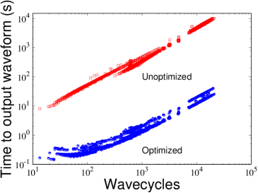
Figure 1: Performance benchmarks: Left panel: plots speedup factor versus number of wavecycles in the binary inspiral. Measuring the number of wavecycles allows us to compactly display the results of the benchmark tests without explicit reference to mass or spin. Right panel: plots the number of wavecycles versus the time taken to output the waveform. Note that the speedup factor in the left panel is simply the ratio of the curves in the right panel.

We would like to measure an average speedup based on the four surveys. As in [20], we define an overall speedup factor as a waveform cycle-weighted average

$$\mathcal{S}=\frac{\sum_{i}\mathcal{S}_{i}N_{i}}{\sum_{i}N_{i}}$$

where $\mathcal{S}_{i}$ is the speedup factor for generating the $i^{\text{th}}$ waveform and $N_{i}$ is the number of wavecycles in the $i^{\text{th}}$ waveform. We found $\mathcal{S}\sim 340$. This reduces the time necessary for a black hole binary PE run from $\mathord{\sim}$100 years (with v3_preopt) to $\mathord{\sim}$8 months (with v3_Opt). We expect lower mass PE runs will be possible on similar timescales with additional optimizations.

4 Conclusions and Future Work

Anticipating the potential detection by Advanced LIGO of significantly precessing compact binaries, we have optimized v3 to make costly precessing-waveform-approximant-based data analysis applications like PE possible in a reasonable amount of time. If an efficient 8D ROM is found, such optimizations will make the construction of this ROM faster. After migrating v2/v4 optimizations to v3, we further optimized partial derivatives of the Hamiltonian using a GAD scheme. This resulted in waveforms that are faithful to v3, as evidenced by faithfulness increasing to 1 as ODE tolerance decreases. We achieved an average overall speedup of $\mathord{\sim}340$x, ranging from $\mathord{\sim}120$x for GW150914-like black hole binaries to $\mathord{\sim}630$x for black hole-neutron star binaries. We expect that further optimizations are possible, achieving an additional speedup factor of at least $\mathord{\sim}$3x. Future work will focus on transforming Cartesian coordinates to spherical coordinates to lower sampling rates even more during ODE solving and integration.

References

References

- [1] B. P. Abbott, R. Abbott, T. D. Abbott, M. R. Abernathy, F. Acernese, K. Ackley, C. Adams, T. Adams, P. Addesso, R. X. Adhikari, et al. Observation of Gravitational Waves from a Binary Black Hole Merger. Phys. Rev. Lett., 116(6):061102:1–16, 2016.
- [2] B. P. Abbott, R. Abbott, T. D. Abbott, M. R. Abernathy, F. Acernese, K. Ackley, C. Adams, T. Adams, P. Addesso, R. X. Adhikari, et al. GW151226: Observation of Gravitational Waves from a 22-Solar-Mass Binary Black Hole Coalescence. Phys. Rev. Lett., 116(24):241103:1–14, 2016.
- [3] B. P. Abbott, R. Abbott, T. D. Abbott, F. Acernese, K. Ackley, C. Adams, T. Adams, P. Addesso, R. X. Adhikari, V. B. Adya, et al. GW170104: Observation of a 50-Solar-Mass Binary Black Hole Coalescence at Redshift 0.2. Phys. Rev. Lett., 118(22):221101:1–17, 2017.
- [4] The LIGO Scientific Collaboration, the Virgo Collaboration, B. P. Abbott, R. Abbott, T. D. Abbott, F. Acernese, K. Ackley, C. Adams, T. Adams, P. Addesso, and et al. GW170608: Observation of a 19-solar-mass Binary Black Hole Coalescence. ArXiv e-prints, 2017.
- [5] B. P. Abbott, R. Abbott, T. D. Abbott, F. Acernese, K. Ackley, C. Adams, T. Adams, P. Addesso, R. X. Adhikari, V. B. Adya, and et al. GW170814: A Three-Detector Observation of Gravitational Waves from a Binary Black Hole Coalescence. Physical Review Letters, 119(14):141101, 2017.
- [6] B. P. Abbott, R. Abbott, T. D. Abbott, F. Acernese, K. Ackley, C. Adams, T. Adams, P. Addesso, R. X. Adhikari, V. B. Adya, and et al. GW170817: Observation of Gravitational Waves from a Binary Neutron Star Inspiral. Physical Review Letters, 119(16):161101, 2017.
- [7] The LIGO Scientific Collaboration. LALSuite: LSC Algorithm Library Suite, 2016. https://www.lsc-group.phys.uwm.edu/daswg/projects/lalsuite.html.
- [8] J. Veitch, V. Raymond, B. Farr, W. Farr, P. Graff, S. Vitale, B. Aylott, K. Blackburn, N. Christensen, M. Coughlin, W. Del Pozzo, F. Feroz, J. Gair, C.-J. Haster, V. Kalogera, T. Littenberg, I. Mandel, R. O’Shaughnessy, M. Pitkin, C. Rodriguez, C. Röver, T. Sidery, R. Smith, M. Van Der Sluys, A. Vecchio, W. Vousden, and L. Wade. Parameter estimation for compact binaries with ground-based gravitational-wave observations using the LALInference software library. Phys. Rev. D, 91(4):042003:1–25, 2015.
- [9] Y. Pan, A. Buonanno, A. Taracchini, L. E. Kidder, A.H. Mroué, H. P. Pfeiffer, M. A. Scheel, and B. Szilágyi. Inspiral-merger-ringdown waveforms of spinning, precessing black-hole binaries in the effective-one-body formalism. Phys. Rev. D, 89(8):084006:1–18, 2014.
- [10] A. Buonanno and T. Damour. Effective one-body approach to general relativistic two-body dynamics. Phys. Rev. D, 59(8):084006:1–24, 1999.
- [11] A. Buonanno, Y. Chen, and T. Damour. Transition from inspiral to plunge in precessing binaries of spinning black holes. Phys. Rev. D, 74(10):104005:1–26, 2006.
- [12] L. Santamaría, F. Ohme, P. Ajith, B. Brügmann, N. Dorband, M. Hannam, S. Husa, P. Mösta, D. Pollney, C. Reisswig, E. L. Robinson, J. Seiler, and B. Krishnan. Matching post-Newtonian and numerical relativity waveforms: Systematic errors and a new phenomenological model for nonprecessing black hole binaries. Phys. Rev. D, 82(6):064016:1–21, 2010.
- [13] M. Hannam, P. Schmidt, A. Bohé, L. Haegel, S. Husa, F. Ohme, G. Pratten, and M. Pürrer. Simple Model of Complete Precessing Black-Hole-Binary Gravitational Waveforms. Phys. Rev. Lett., 113(15):151101:1–5, 2014.
- [14] S. Husa, S. Khan, M. Hannam, M. Pürrer, F. Ohme, X. Jiménez Forteza, and A. Bohé. Frequency-domain gravitational waves from nonprecessing black-hole binaries. I. New numerical waveforms and anatomy of the signal. Phys. Rev. D, 93(4):044006:1–19, 2016.
- [15] S. Khan, S. Husa, M. Hannam, F. Ohme, M. Pürrer, X. Jiménez Forteza, and A. Bohé. Frequency-domain gravitational waves from nonprecessing black-hole binaries. II. A phenomenological model for the advanced detector era. Phys. Rev. D, 93(4):044007:1–27, 2016.
- [16] S. Babak, A. Taracchini, and A. Buonanno. Validating the effective-one-body model of spinning, precessing binary black holes against numerical relativity. Phys. Rev. D, 95(2):024010, January 2017.
- [17] M. Pürrer. Frequency domain reduced order model of aligned-spin effective-one-body waveforms with generic mass ratios and spins. Phys. Rev. D, 93(6):064041:1–15, 2016.
- [18] S. E. Field, C. R. Galley, J. S. Hesthaven, J. Kaye, and M. Tiglio. Fast prediction and evaluation of gravitational waveforms using surrogate models. Phys. Rev. X, 4(3):031006:1–21, 2014.
- [19] S. E. Field, C. R. Galley, and E. Ochsner. Towards beating the curse of dimensionality for gravitational waves using reduced basis. Phys. Rev. D, 86(8):084046:1–7, 2012.
- [20] C. Devine, Z. B. Etienne, and S. T. McWilliams. Optimizing spinning time-domain gravitational waveforms for advanced LIGO data analysis. Class. Quantum Grav., 33(12):125025:1–15, 2016.
- [21] A. Taracchini, A. Buonanno, Y. Pan, T. Hinderer, M. Boyle, D. A. Hemberger, L. E. Kidder, G. Lovelace, A. H. Mroué, H. P. Pfeiffer, M. A. Scheel, B. Szilágyi, N. W. Taylor, and A. Zenginoglu. Effective-one-body model for black-hole binaries with generic mass ratios and spins. Phys. Rev. D, 89(6):061502:1–6, 2014.
- [22] R. M. Stallman and GCC DeveloperCommunity. Using The Gnu Compiler Collection. 51 Franklin Street, Fifth Floor, Boston, MA 02110-1301 USA, 2015.
- [23] Intel. User and Reference Guide for the Intel® C++ Compiler 15.0, 2014. https://software.intel.com/en-us/compiler_15.0_ug_c.
- [24] Wolfram Research, Inc. Mathematica 10.4. Champaign, Illinois, 2016. https://www.wolfram.com.
- [25] N. Limare. Floating-Point Math Speed vs Precision, 2014. http://nicolas.limare.net/pro/notes/2014/12/16_math_speed/.
- [26] W. H. Press, S. A. Teukolsky, W. T. Vetterling, and B. P. Flannery. Numerical Recipies: The Art of Scientific Computing - Third Edition. Cambridge University Press, 3rd edition, 2007. http://numerical.recipies.
- [27] A. Nitz, I. Harry, C. M. Biwer, D. Brown, J. Willis, T. Dal Canton, L. Pekowsky, T. Dent, A. R. Williamson, C. Capano, et al. ligo-cbc/pycbc: O2 Production Release 11, 2017. https://doi.org/10.5281/zenodo.556097.
- [28] T. Dal Canton, A. H. Nitz, A. P. Lundgren, A. B. Nielsen, D. A. Brown, T. Dent, I. W. Harry, B. Krishnan, A. J. Miller, K. Wette, K. Wiesner, and J. L. Willis. Implementing a search for aligned-spin neutron star-black hole systems with advanced ground based gravitational wave detectors. Phys. Rev. D, 90(8):082004:1–17, 2014.
- [29] S. A. Usman, A. H. Nitz, I. W. Harry, C. M. Biwer, D. A. Brown, M. Cabero, C. D. Capano, T. Dal Canton, T. Dent, S. Fairhurst, M. S. Kehl, D. Keppel, B. Krishnan, A. Lenon, A. Lundgren, A. B. Nielsen, L. P. Pekowsky, H. P. Pfeiffer, P. R. Saulson, M. West, and J. L. Willis. The PyCBC search for gravitational waves from compact binary coalescence. Class. Quantum Grav., 33(21):215004:1–25, 2016.
- [30] A. Bohé, L. Shao, A. Taracchini, A. Buonanno, S. Babak, I. W. Harry, I. Hinder, S. Ossokine, M. Pürrer, V. Raymond, T. Chu, H. Fong, P. Kumar, H. P. Pfeiffer, M. Boyle, D. A. Hemberger, L. E. Kidder, G. Lovelace, M. A. Scheel, and B. Szilágyi. Improved effective-one-body model of spinning, nonprecessing binary black holes for the era of gravitational-wave astrophysics with advanced detectors. Phys. Rev. D, 95(4):044028:1–29, 2017.
- [31] LSC. Advanced LIGO anticipated sensitivity curves, 2010. https://dcc.ligo.org/LIGO-T0900288/public.