Unified Phase Diagram of Antiferromagnetic $\mathrm{SU}(N)$ Spin Ladders

Abstract

Motivated by near-term experiments with ultracold alkaline-earth atoms confined to optical lattices, we establish numerically and analytically the phase diagram of two-leg $\mathrm{SU}(N)$ spin ladders. Two-leg ladders provide a rich and highly non-trivial extension of the single chain case on the way towards the relatively little explored two dimensional situation. Focusing on the experimentally relevant limit of one fermion per site, antiferromagnetic exchange interactions, and $2\leq N\leq 6$, we show that the phase diagrams as a function of the interchain (rung) to intrachain (leg) coupling ratio $J_{\perp}/J_{\|}$ strongly differ for even vs. odd $N$. For even $N=4$ and $6$, we demonstrate that the phase diagram consists of a single valence bond crystal (VBC) with a spatial period of $N/2$ rungs. For odd $N=3$ and $5$, we find surprisingly rich phase diagrams exhibiting three distinct phases. For weak rung coupling, we obtain a VBC with a spatial period of $N$ rungs, whereas for strong coupling we obtain a critical phase related to the case of a single chain. In addition, we encounter intermediate phases for odd $N$, albeit of a different nature for $N=3$ as compared to $N=5$. For $N=3$, we find a novel gapless intermediate phase with $J_{\perp}$-dependent incommensurate spatial fluctuations in a sizeable region of the phase diagram. For $N=5$, there are strong indications for a narrow potentially gapped intermediate phase, whose nature is not entirely clear. Our results are based on (i) field theoretical techniques, (ii) qualitative symmetry considerations, and (iii) large-scale density matrix renormalization group (DMRG) simulations keeping beyond a million of states by fully exploiting and thus preserving the $\mathrm{SU}(N)$ symmetry.

I Introduction

Two-leg spin ladders have been a focus of much theoretical and experimental work over more than two decades. This strong interest stems in part from purely theoretical reasons Dagotto and Rice (1996); Gogolin et al. (1998); Giamarchi (2004); Schmidiger et al. (2013) but is also motivated by experimental realizations Azuma et al. (1994); Caron et al. (2011); Luo et al. (2013). These simple magnetic quantum systems might also be employed as quantum simulators for fundamental theories of particle and many body physics Ward et al. (2013); Lake et al. (2010); Jördens et al. (2008). From a theoretical point of view, ladder systems provide the simplest non-trivial step away from well-understood purely one-dimensional systems to higher dimensions. Quite interestingly, a confinement of fractional quantum number excitations can be investigated in simple two-leg spin ladders. In the case of two spin-half $\mathrm{SU}(2)$ Heisenberg chains coupled by an antiferromagnetic spin-exchange interaction, the theory predicts that gapless fractional spin-half excitations of individual chains (spinons) are confined into gapful spin-1 excitations (triplons) even by an infinitesimal interchain coupling Shelton et al. (1996). Experiments provide evidence for such confinement Schmidiger et al. (2013); Lake et al. (2010).

In condensed matter systems, the SU(2) symmetry is quite natural due to the mostly electronic origin of the quantum magnetism. In recent years it has, however, been theoretically proposed Cazalilla et al. (2009); Gorshkov et al. (2010) to create $\mathrm{SU}(N)$ quantum magnets by loading fermionic alkaline-earth-like atoms into optical lattices and driving them into the Mott insulating regimes. Considerable experimental progress by several groups Zhang et al. (2014); Scazza et al. (2014); Cappellini et al. (2014); Pagano et al. (2014); Hofrichter et al. (2016) shows this to be an interesting further avenue for quantum magnetism. Experiments can realize two-leg $\mathrm{SU}(N)$ spin ladders from ultracold alkaline-earth or ytterbium atoms. The ladder geometry may be realized by double-well optical lattices similar to those in two-leg Bose-Hubbard models with cold atoms Sebby-Strabley et al. (2006); Danshita et al. (2007); Atala et al. (2014).

When dealing with fermions, a major challenge consists in cooling them down to reach ground-state properties. In that context, $\mathrm{SU}(N)$ symmetry is appealing since a larger number of flavors ($N$) allows to reach lower temperature (or entropy) Hazzard et al. (2012). Therefore short-distance correlations characteristic of Heisenberg physics should be accessible, e.g. as discussed for one-dimensional systems Messio and Mila (2012); Bonnes et al. (2012) or even two-dimensional $\mathrm{SU}(N)$ Hubbard models Cai et al. (2013). Recent developments of quantum gas microscopy also promise increased access to measure local quantities Jördens et al. (2008); Cheuk et al. (2015); Parsons et al. (2015); Greif et al. (2016) or short-distance correlations Greif et al. (2011); Parsons et al. (2016).

From the theoretical point of view, the one-dimensional $\mathrm{SU}(N)$ Heisenberg chain is well characterized thanks to the exact solution Sutherland (1975), and it represents a critical state quite analogous to the $\mathrm{SU}(2)$ case. When considering more general single-band Hubbard models of $\mathrm{SU}(N)$ fermions, the phase diagram becomes already richer with the emergence of different kind of Mott insulating phases or dimerized phases Capponi et al. (2016). Moreover, it appears that additional degrees of freedom (such as an orbital one) could give rise to even more exotic phases, such as symmetry-protected topological ones Capponi et al. (2016). In two dimensions, there has been a large number of studies devoted to various lattices and $N$. Restricting to ‘minimal’ models where, at each site, the local Hilbert space corresponds to the fundamental $\mathrm{SU}(N)$ representation (i.e. one particle per site in a fermionic language), analytical arguments Hermele et al. (2009); Hermele and Gurarie (2011) have triggered a series of numerical investigations which have proposed, for instance, that the ground-state can break spontaneously the $\mathrm{SU}(N)$ symmetry Tóth et al. (2010); Bauer et al. (2012) or break some lattice symmetries Corboz et al. (2013); Nataf et al. (2016) or break both symmetries Corboz et al. (2011), or exhibit an algebraic spin-liquid phase Corboz et al. (2012). Now, it has to be mentioned that the two-dimensional simulations remain quite challenging, so that a deep and detailed understanding of the two-leg ladder case could shed some light on non-trivial effects when going from one to two dimensions. The inherent difficulty to numerically simulate large $N$ in $\mathrm{SU}(N)$ could also be a further niche for quantum simulations. Last but not least, we will argue that a minimal model is experimentally feasible since it requires to have $\mathrm{SU}(N)$ symmetry, one particle per site (which is good to prevent losses), and ladder geometry, all of which have been realized in experiments.

The paper is organized as follows. In the remainder of this section, we define the model system (subsection I.1), and give a brief overview of what is known about the phase diagrams of $\mathrm{SU}(N)$ ladder, the open questions and a summary of our resulting phase diagram (subsection I.2). In Sec. II we present our analytical analysis for weak rung coupling based on conformal field theory (CFT) and mean field theory. In Sec. III we present our exact numerical results for the full range of antiferromagnetic rung coupling based on the density matrix renormalization group (DMRG). In Sec. IV we give a summary, followed by an outlook.

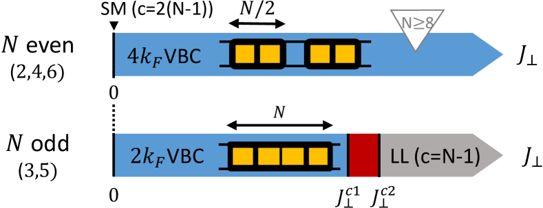
Figure 1: (Color online) Phase diagrams of two-leg $\mathrm{SU}(N)$ antiferromagnetic ladders for $N\leq 6$ vs. $J_{\perp}$, setting $J_{\|}=1$. At $J_{\perp}=0$, all ladders are critical [two decoupled Sutherland models (SM), with total central charge $c=2\times(N-1)$]. For finite $J_{\perp}>0$, for even $N$ a single symmetry-broken $4k_{F}$ valence-bond crystal (VBC) phase with an $N$-site plaquette is found, which for $N=2$ reduces to a trivial nondegenerate rung singlet phase (note that for $N\geq 8$ and large $J_{\perp}$, a critical phase with $c=N-1$ is expected even for even $N$). For odd $N$, in stark contrast, we find three phases. For small $J_{\perp}$ a $2k_{F}$-VBC, for large $J_{\perp}$ a critical Luttinger liquid (LL) with central charge $c=N-1$, and an intermediate phase. This intermediate phase for $N=3$ ($J_{\perp}\in[\sim 1,1.562]$) is incommensurate, and for $N=5$ ($J_{\perp}\in[0.581,0.596]$) is reminiscent of topological phases.

I.1 Model system

Motivated by ultracold atomic gases of alkaline-earth-like fermionic atoms, such as Yb ($N$ up to $6$) and Sr ($N$ up to $10$), confined to an optical lattice, we start our description with an $N$-species single-band fermionic Hubbard model in a two-leg ladder geometry:

$${\cal H}_{\mathrm{Hubbard}} = \sum_{\ell x}\bigl{(}-\mu\,n_{\ell x}+\tfrac{U}{2}n_{\ell x}(n_{\ell x}-1)\bigr{)}$$

$$- \sum_{x\alpha}\Bigl{(}t_{\perp}c^{\dagger}_{1x\alpha}c^{\phantom{\dagger}}_{2x\alpha}+t_{\parallel}\sum_{\ell}c^{\dagger}_{\ell x\alpha}c^{\phantom{\dagger}}_{\ell,x+1,\alpha}+\mathrm{H.c.}\Bigr{)},$$

where $x$ denotes the position along the ladder, $\ell\in\{1,2\}$ labels the two legs, and $c^{\dagger}_{\ell x\alpha}$ and $c^{\phantom{\dagger}}_{\ell x\alpha}$ are the fermionic creation and annihilation operators of a fermionic atom at lattice position $(x,\ell)$ in the internal state $\alpha$, and $n_{\ell x}=\sum_{\alpha}c^{\dagger}_{\ell x\alpha}c^{\phantom{\dagger}}_{\ell x\alpha}$. The hopping amplitudes along the leg (rung) are labeled as $t_{\parallel}$ ($t_{\perp}$), respectively, and can easily be controlled in experiments by the strength of the optical lattice. The on-site interaction $U>0$ is assumed to be positive, throughout. We assume the chemical potential $\mu$ to be chosen such that we have a filling of one fermion per site (and therefore Fermi wave-vector $k_{F}\equiv\pi/N$) . Then the limit of strong on-site repulsion $U\gg t_{\parallel},t_{\perp}$ leads to a Mott insulator, where the charge fluctuations are suppressed, while the only remaining degrees of freedom are the $\mathrm{SU}(N)$ spins at each lattice site. Their local state space is described by a single multiplet of dimension $N$ that transforms in the fundamental irreducible representation of the $\mathrm{SU}(N)$ symmetry group which, in the language of Young tableaux, corresponds to a single box ( ${\tiny\yng(1)}$ ). In second order perturbation theory in the hopping, virtual charge fluctuations induce an effective dynamics in the spin-only description, which is called the $\mathrm{SU}(N)$ Heisenberg model:

$${\cal H}_{\mathrm{ladder}}=J_{\parallel}\sum_{\ell,x,A}S^{A}_{\ell,x}S^{A}_{\ell,x+1}+J_{\perp}\sum_{x,A}S^{A}_{1,x}S^{A}_{2,x}\text{ ,}$$ (2)

where $S^{A}_{\ell,x}$ with $A=1,\ldots,N^{2}-1$ denote the $\mathrm{SU}(N)$ spin operators i.e. the generators of the $\mathrm{SU}(N)$ Lie algebra. The antiferromagnetic exchange coupling constants $J_{\parallel}$ and $J_{\perp}$ are related to the parameters of the underlying Hubbard model as $J_{\parallel(\perp)}=4\,(t_{\parallel(\perp)})^{2}/U$ in the leading order of perturbation theory. By using the generalized Pauli identity (see App. A),

$$S_{i}\cdot S_{j}\equiv\sum_{A}S^{A}_{i}S^{A}_{j}=\tfrac{1}{2}(P_{i,j}-\tfrac{1}{N})\text{ ,}$$ (3)

with the permutation operator $P_{i,j}=\sum_{\alpha,\beta}|\alpha_{i},\beta_{j}\rangle\langle\beta_{i},\alpha_{j}|$ for sites $i\equiv(\ell,x)$, the spin Hamiltonian can be rewritten as a sum of two-site permutations (up to constant terms), if the spin operators act on the fundamental representation, as is the case here. With $\langle P_{i,j}\rangle\in[-1,1]$, the generalized “spin-spin” correlations are constrained to the range $\langle S_{i}\cdot S_{j}\rangle\in[-\tfrac{1}{2},+\tfrac{1}{2}]-\tfrac{1}{2N}$. Conversely, the symmetric (+) or antisymmetric (-) weight on the bond between sites $i$ and $j$ can be simply obtained by

$$p_{ij}^{\pm}\equiv\langle\tfrac{1}{2}(1\pm P_{ij})\rangle=\tfrac{1}{2}\pm\bigl{(}\langle S_{i}\cdot S_{j}\rangle+\tfrac{1}{2N}\bigr{)}\text{ .}$$ (4)

In this paper we now proceed to establish the phase diagrams of the spin Hamiltonian ${\cal H}_{\mathrm{ladder}}$ in Eq. (2) for $N$ varying from $2$ to $6$ analytically and numerically for the full range of $J_{\perp}/J_{\|}$ in the experimentally accessible antiferromagnetic regime $J_{\|},J_{\perp}\geq 0$. This ties together partly available literature for small and large ladder coupling $J_{\perp}$ Affleck (1988a); Dufour et al. (2015); Capponi et al. (2016); van den Bossche et al. (2001); Lecheminant and Tsvelik (2015); James et al. (2017), and the known case of $N=2$ Shelton et al. (1996). We also speculate on the physics for larger $N$. While it would be desirable to explore $N$ up to $10$ for experiments on Sr atoms, for the Heisenberg model as well as for the Hubbard model for the whole $U>0$ range, these goals are currently out of reach for exact numerical approaches. After all, the models inherit the numerical complexity of $N$-flavor many-body systems. For $\mathrm{SU}(N)$ symmetric models this manifests itself predominantly in the fact that typical individual multiplets grow exponentially in size with increasing $N$ (in practice, $d\lesssim 10^{N-1}$).

I.2 Overview of the Phase Diagrams

In this paper, we determine the phase diagrams as a function of an antiferromagnetic interchain exchange interaction $J_{\perp}>0$ for up to $N=6$. We work at zero temperature, fixing $J_{\parallel}=1$ as the unit of energy, unless stated otherwise. The goal of this section is to present the key results of this paper in a compact way and to refer the reader to the following sections for a more detailed presentation organized by the technique.

A schematic summary of our result is presented in Fig. 1. These phase diagrams have been obtained using field theoretical results detailed in Sec. II and large-scale DMRG simulations with results detailed in Sec. III.

Let us start with some known limits of these phase diagrams and a statement of the hitherto open questions. The case $N=2$ corresponds to the well studied $\mathrm{SU}(2)$, $S{=}1/2$ two-leg spin ladder Shelton et al. (1996), which we include for completeness only. It has been established that the entire $J_{\perp}>0$ range forms one phase which is continuously connected to the non-degenerate product state of rung singlets which one obtains in the limit $J_{\perp}\rightarrow+\infty$. Hence the name ”rung singlet phase” encountered in the literature. This phase has a unique ground state on open and periodic systems and a gap to all excitations.

A different established limiting case is the strong coupling limit, i.e. $J_{\perp}\rightarrow+\infty$ for all $N$, where the system can be described effectively as a single $\mathrm{SU}(N)$ Heisenberg chain:

$${\cal H}_{\mathrm{chain}}=J_{\mathrm{chain}}\sum_{x,A}\tilde{S}^{A}_{x}\tilde{S}^{A}_{x+1}\text{ ,}$$ (5)

albeit with different local spin degrees of freedom, in that $\tilde{S}^{A}_{x}$ acts within the two-box antisymmetric representation ( ${\tiny\yng(1,1)}$ ) of dimension $N(N-1)/2$. The exchange constant $J_{\mathrm{chain}}$ is proportional to $J_{\parallel}$ in general. While this is a trivial Hamiltonian and state for $N=2$ as discussed in the paragraph before, the situation is much richer for larger $N$ where we have to distinguish based on the parity of $N$ Affleck (1988a); Dufour et al. (2015): for even $N=4$ or $N=6$, the chain will spontaneously dimerize or trimerize, respectively, which in the original ladder language corresponds to $2\times 2=4$-site and $3\times 2=6$-site plaquette formation (see Fig. 1) Capponi et al. (2016); Dufour et al. (2015). For the $\mathrm{SU}(4)$ case, the plaquette formation has already been reported for a ladder when $J_{\perp}$ is large van den Bossche et al. (2001). For odd $N>1$ and even $N>6$ (see App. D of Lecheminant and Tsvelik (2015) and Ref. Dufour et al. (2015), and also Fig. 1), the chain remains critical in the $\mathrm{SU}(N)$₁ Wess-Zumino-Novikov-Witten (WZNW) universality class, which corresponds to a highly symmetric $(N-1)$-component Luttinger liquid (LL).

Finally the last (partially) known starting point is the weak coupling limit. For $J_{\perp}=0$, the system decouples into two copies of $\mathrm{SU}(N)$ Heisenberg spin chains, one on each leg, with the spins in the fundamental representation. The individual spin chain models are also known as $\mathrm{SU}(N)$ Sutherland models Sutherland (1975). The Sutherland model is integrable by means of Bethe ansatz and displays quantum critical behavior in the $\mathrm{SU}(N)$₁ WZNW universality class with central charge $c=N-1$ Sutherland (1975); Affleck (1988a). Recent field theoretical work by two of the present authors Lecheminant and Tsvelik (2015) has established that for all even $N$ an infinitesimal interchain coupling $J_{\perp}>0$ is expected to give a gapped phase of the valence bond crystal (VBC) type. A cartoon description of these states is given by an array of $\mathrm{SU}(N)$ singlets consisting of $N$ spins on $N/2$ consecutive rungs (see Fig. 1). For even $N>2$ this therefore amounts to a state with broken translation symmetry along the ladders and an ensuing ground state degeneracy of $N/2$ in the thermodynamic limit. The system is expected to exhibit gaps for magnetic and non-magnetic excitations beyond the ground state manifold. These types of VBCs with a unit cell of $N$ spins in a $N/2\times 2$ geometry may also be called a “$4k_{F}$ VBC” since their modulation wave vector $2\pi/(N/2)=4\pi/N$ corresponds to four times $k_{F}$, having $k_{F}=\pi/N$. The odd $N$ case is also unstable upon switching on a finite $J_{\perp}$. However the nature of the resulting phases were not clear so far. In this paper we show analytically that for $N=3$ the system forms a different VBC type as compared to the even $N$ case. Here a “$2k_{F}$ VBC” forms with a unit cell comprising $2N$ spins arranged in a $N\times 2$ building block along the ladder (see Fig. 1). This picture is confirmed by large scale DMRG simulations. Our numerical results show that the $2k_{F}$ VBC phase also persists for $N=5$ at weak coupling.

Aside from this review of known limiting cases, the physics in the entire intermediate coupling regime for all $N>2$ is basically unexplored. From a qualitative point of view it is possible that the physics for even $N\leq 6$ is adiabatically connected from weak to strong coupling, although this has not been demonstrated before. However the phases at weak and strong coupling for odd $N=3,5$ manifestly differ, and thus require at least one phase transition in between.

In the following we demonstrate that the even cases $N=4$ and $N=6$ are indeed forming a single $4k_{F}$-VBC phase for all $J_{\perp}>0$, while the odd cases $N=3$ and $N=5$ exhibit extended intermediate phases between the $2k_{F}$-VBC phases at small $J_{\perp}$ and the critical regime at strong rung coupling. The intermediate phase for $N=3$ is of a novel $\mathrm{SU}(N)$ incommensurate type, where the $J_{\perp}$-dependent incommensuration is driven by the relative population density of the symmetric ( ${\tiny\yng(2)}$ ) and antisymmetric ( ${\tiny\yng(1,1)}$ ) rung multiplets. In the case $N=5$ the intermediate phase is quite narrow, potentially gapped, and generally of rather different nature as compared to the $N=3$ intermediate phase.

II Weak rung coupling results $J_{\perp}\gtrsim 0$:
Field theoretical approach

In this section we start the construction of the phase diagrams coming from the decoupled chain limit $J_{\perp}=0$. Using field theoretical methods we establish the fate of this singular starting point after switching on a small antiferromagnetic rung coupling $J_{\perp}$. Previously established results for all even $N$ are reviewed. Then the case $N=3$ is treated explicitly.

II.1 Continuum description

As stated above, at $J_{\perp}=0$, model (2) becomes two decoupled $\mathrm{SU}(N)$ Sutherland models with a total central charge $c=2(N-1)$. The low-energy properties of the Sutherland model can be obtained by starting from the U($N$) Hubbard model at $1/N$ filling with a large repulsive $U$ interaction Affleck (1986, 1988a); Assaraf et al. (1999); Manmana et al. (2011). At low energy below the charge gap, the $\mathrm{SU}(N)$ operators in the continuum limit are described by Affleck (1986, 1988a):

$$S^{A}_{\ell,x}\simeq J^{A}_{\ell L}(x)+J^{A}_{\ell R}(x)+e^{i2k_{F}x}i\lambda\;\mathrm{Tr}\bigl{(}g_{\ell}(x)T^{A}\bigr{)}+\mathrm{H.c.}\text{ ,}$$ (6)

where $J^{A}_{\ell L,R}$ are the left and right $\mathrm{SU}(N)_{1}$ currents, and $T^{A}$ are generators of the su($N$) algebra in the fundamental representation (Gell-Mann matrices) normalized such that $\mathrm{Tr}(T^{A}T^{B})=\delta^{AB}/2$. The $2k_{F}$ term involves the $\mathrm{SU}(N)_{1}$ WZNW field $g_{\ell}$ with scaling dimension $\frac{N-1}{N}$. The non-universal real constant $\lambda$ corresponds to the average over the charge degrees of freedom in the large $U$ limit.

The continuum limit of the two-leg $\mathrm{SU}(N)$ spin ladder (2) is then described by the low-energy Hamiltonian:

$${\cal H} = {\cal H}^{(1)}_{\mathrm{SU}(N)_{1}}+{\cal H}^{(2)}_{\mathrm{SU}(N)_{1}}+\lambda_{1}\int dx\;\bigl{[}\mathrm{Tr}(g_{1}g_{2}^{+})+\mathrm{H.c.}\bigr{]}$$ (7)

$$+ \lambda_{2}\int dx\;\bigl{[}\mathrm{Tr}g_{1}\mathrm{Tr}g_{2}^{+}+\mathrm{H.c.}\bigr{]}\text{ ,}$$

where ${\cal H}^{(\ell)}_{\mathrm{SU}(N)_{1}}$ denotes the Hamiltonian of the $\mathrm{SU}(N)_{1}$ CFT for the $\ell=1,2$ decoupled chain, and $\lambda_{1}=J_{\perp}\lambda^{2}/2$, $\lambda_{2}=-\lambda_{1}/N$. Model (7) describes two $\mathrm{SU}(N)_{1}$ WZNW models perturbed by two strongly relevant perturbations with the same scaling dimension $2(N-1)/N<2$. Since these perturbations are strongly relevant, we have not included in Eq. (7) the marginal current-current interaction. The effective field theory (7) can be simplified by exploiting the fact that when $J_{\perp}\neq 0$ the continuous symmetry group of model (2) is $\mathrm{SU}(N)\times{\mathbb{Z}}_{2}$ making it more natural to consider the following conformal embedding Francesco et al. (1997):

$$\mathrm{SU}(N)_{1}\times\mathrm{SU}(N)_{1}\sim\mathrm{SU}(N)_{2}\times\mathbb{Z}_{N}\text{ .}$$ (8)

Here the $\mathrm{SU}(N)_{2}$ CFT has central charge $c=2\tfrac{N^{2}-1}{N+2}$ and ${\mathbb{Z}}_{N}$ is the parafermionic CFT with central charge $c=\frac{2(N-1)}{N+2}$. It describes universal properties of the phase transition of the ${\mathbb{Z}}_{N}$ generalization of the 2D Ising model Zamolodchikov and Fateev (1985). The low-energy Hamiltonian (7) can then be expressed in the new basis and reads Lecheminant and Tsvelik (2015)

$${\cal H} = {\cal H}_{\mathrm{SU}(N)_{2}}+\bigl{[}{\cal H}_{{\mathbb{Z}}_{N}}-g\int dx\;\left(\Psi_{1L}\Psi_{1R}+\mathrm{H.c.}\right)\bigr{]}$$ (9)

$$+ \lambda_{2}\int dx\;\mathrm{Tr}(\Phi_{\rm adj})\bigl{(}\sigma_{2}+\sigma_{2}^{\dagger}\bigr{)}\text{ ,}$$

where $g=-NJ_{\perp}\lambda^{2}/8\pi^{2}$ and $\lambda_{2}=-J_{\perp}\lambda^{2}/2N$. The effective field theory (9) contains two different sectors, the $\mathrm{SU}(N)$ singlet one in square brackets, and the magnetic one, which depends on the $\mathrm{SU}(N)$ degrees of freedom. These sectors are coupled by the last term with coupling constant $\lambda_{2}$. Operators ${\cal H}_{\mathrm{SU}(N)_{2}}$ and $\Phi_{\rm adj}$ act in the $\mathrm{SU}(N)$ sector; the former one is the Hamiltonian of the $\mathrm{SU}(N)_{2}$ CFT and the latter one is a primary field with scaling dimension $\Delta_{\rm adj}=\tfrac{2N}{N+2}$ which transforms in the adjoint representation of the $\mathrm{SU}(N)$. In Eq. (9), ${\cal H}_{{\mathbb{Z}}_{N}}$ is the Hamiltonian of ${\mathbb{Z}}_{N}$ CFT which is generated by the ${\mathbb{Z}}_{N}$ parafermion currents $\Psi_{1L,R}$ with conformal weights $h,{\bar{h}}=\tfrac{N-1}{N}$. Operators $\sigma_{k}$ ($k=1,\ldots N-1$) are the ${\mathbb{Z}}_{N}$ order parameter fields with scaling dimensions $\Delta_{k}=\tfrac{k(N-k)}{N(N+2)}$. Fields with $k>1$ are generated by fusion of the fundamental order parameter field $\sigma_{1}$; $\sigma_{k}$ take non-zero expectation values in the phase which spontaneously breaks the ${\mathbb{Z}}_{N}$ symmetry.

II.2 Weak-coupling phase diagram

The two perturbations in Eq. (9) are relevant with the same scaling dimension $\tfrac{2(N-1)}{N}<2$. The crucial difference between $\mathrm{SU}(2)$ and $\mathrm{SU}(N>2)$ cases stems from two facts. First, for $N=2$, $\sigma_{2}$ is just an identity operator and hence the two sectors of the theory remain decoupled  Shelton et al. (1996). Second, for $N=2$, $\Psi_{1L,R}$ are Majorana fermions and $\Phi_{\rm adj}$ is also bilinear in Majorana fermions. In this respect, model (9) can be expressed in terms of four massive Majorana fermions which account for the emergence of non-denegerate gapful phases for any sign of $J_{\perp}$ Shelton et al. (1996). The situation is much more involved in the case of $N>2$ due to the coupling of the magnetic and the singlet sectors. Hence a different physical picture is expected. One way to determine the low-energy properties of model (9) is to use the fact that when $\lambda_{2}=0$, the ${\mathbb{Z}}_{N}$ sector of (9) is an integrable deformation of the ${\mathbb{Z}}_{N}$ parafermions introduced by Fateev Fateev (1991); Fateev and Zamolodchikov (1991). Since the infrared properties of this theory strongly depend on the parity of $N$ we have to consider odd and even cases separately.

II.2.1 Even $N$

For even $N$, a spectral gap is generated for the ${\mathbb{Z}}_{N}$ Fateev model (the expression in the square brackets in (9)) for any sign of $J_{\perp}$. In Ref. Lecheminant and Tsvelik, 2015, two of us have exploited the exact solution of the Fateev model to find the low-energy properties of weakly-coupled $\mathrm{SU}(2n)$ two-leg spin ladder. In the simplest $N=4$ case, we have found the competition between a tetramerized ($2k_{F}$) phase with a four-fold ground state degeneracy and a two-fold degenerate plaquette (dimerized, $4k_{F}$) phase Lecheminant and Tsvelik (2015). In particular, when $|\lambda_{1}|\ll|\lambda_{2}|$, a plaquette phase was predicted. At sufficiently strong $J_{\perp}\gg 1$, we already know that there is spontaneous translation symmetry breaking with the formation of VBC formed with 4-site and 6-site plaquettes respectively for $N=4$ and $N=6$ respectively. However, at weak coupling the field-theory analysis of Ref. Lecheminant and Tsvelik, 2015, has not made it clear which phase wins the competition when both $\lambda_{1}$ and $\lambda_{2}$ are similar in magnitude as it is the case when the interchain coupling $J_{\perp}$ is switched on. Hence it may happen that the latter phase is replaced by a tetramerized phase ($2k_{F}$ VBC). To settle this issue we resort to a numerical investigation in Sec. III.1.

II.2.2 Odd $N$

The strategy of Ref. Lecheminant and Tsvelik (2015) is not applicable for odd $N$ since the physical properties of the integrable Fateev ${\mathbb{Z}}_{N}$ model strongly depend on the sign of its coupling constant $\lambda_{1}$ Fateev (1991); Fateev and Zamolodchikov (1991). In particular, when $J_{\perp}>0$, the ${\mathbb{Z}}_{N}$ Fateev model (9) with $\lambda_{2}=0$ displays an integrable massless renormalization group (RG) flow from the ${\mathbb{Z}}_{N}$ ultraviolet (UV) fixed point to the infrared (IR) one governed by the minimal model ${\cal M}_{N+1}$ CFT with central charge $c=1-\tfrac{6}{(N+2)(N+1)}$ Fateev and Zamolodchikov (1991). In the simplest case, i.e. $N=3$, one has a massless flow from ${\mathbb{Z}}_{3}$ CFT to the ${\cal M}_{4}$ CFT which corresponds to the $c=7/10$ tricritical Ising model (TIM) CFT which describes the critical properties of two-dimensional discrete models with ${\mathbb{Z}}_{2}$ Ising spins $\sigma=\pm 1$ and a vacancy variable $t=0,1$ Francesco et al. (1997). The strategy for odd $N$ is thus to rewrite model (9) in the IR limit by exploiting the existence of the massless RG flow. To this end, we need the UV-IR transmutation of the ${\mathbb{Z}}_{N}$ fields and most importantly the expression of the field $\sigma_{2}+\sigma_{2}^{\dagger}$ at the IR ${\cal M}_{N+1}$ fixed point. Unfortunately, to the best of our knowledge, we are aware of such UV-IR transmutation only in the simplest $N=3$ case. In the odd $N$ case, we can thus only investigate the low-energy properties of the SU(3) spin ladder in this paper. In this respect, the transmutation of the ${\mathbb{Z}}_{3}$ primary fields has been investigated in Ref. Klassen and Melzer, 1993 by means of the thermodynamic Bethe ansatz Zamolodchikov (1991); Klassen and Melzer (1992). The most important one for our study is the UV-IR transmutation of the ${\mathbb{Z}}_{3}$ spin field

$$\sigma=\sigma_{2}^{\dagger},~{}~{}\sigma+\sigma^{+}\rightarrow\epsilon_{\rm TIM},$$ (10)

where $\epsilon_{\rm TIM}$ is the so-called thermal operator of TIM CFT, which has scaling dimension $1/5$ Francesco et al. (1997). We thus deduce the IR limit of model (9) in terms of the fields of the TIM $\times\ \mathrm{SU}(3)_{2}$ CFT:

$${\cal H}={\cal H}_{\mathrm{SU}(3)_{2}}+{\cal H}_{{\rm TIM}}+\kappa\int dx\;\mathrm{Tr}(\Phi_{\rm adj})\;\epsilon_{\rm TIM},$$ (11)

where ${\cal H}_{{\rm TIM}}$ is the Hamiltonian of the TIM CFT and $\kappa\simeq\lambda_{2}<0$ when $J_{\perp}>0$. The interacting part of model (11) is a strongly relevant perturbation with scaling dimension $7/5<2$ which should open a mass gap for both sectors of the theory. To investigate the IR properties of model (11) we resort to a simple mean-field approach to decouple the $\mathrm{SU}(3)_{2}$ and TIM sectors and to exploit the existence of a massive integrable perturbation of the TIM CFT: ${\cal H}_{\rm mf}={\cal H}_{1}+{\cal H}_{2}$ with:

$${\cal H}_{1} = {\cal H}_{{\rm TIM}}+\kappa\int dx\;\langle\mathrm{Tr}(\Phi_{\rm adj})\rangle\;\epsilon_{\rm TIM}$$

$${\cal H}_{2} = {\cal H}_{\mathrm{SU}(3)_{2}}+\kappa\int dx\;\langle\epsilon_{\rm TIM}\rangle\;\mathrm{Tr}(\Phi_{\rm adj})$$ (12)

The excitation spectra of (12) are known. ${\cal H}_{1}$ describes the TIM CFT perturbed by its thermal operator which is a massive integrable field theory for all sign of $\kappa$ Lässig et al. (1991). When $\kappa<0$, we have $\langle\epsilon_{\rm TIM}\rangle>0$ which means, within our conventions, that the underlying 2D TIM belongs to its high-temperature paramagnetic phase where the ${\mathbb{Z}}_{2}$ symmetry is unbroken. The Hamiltonian ${\cal H}_{2}$ of Eq. (12) describes an $\mathrm{SU}(3)_{2}$ CFT perturbed by its adjoint primary field which has been recently studied in Ref. Lecheminant, 2015. A massive behavior occurs when the coupling constant is negative as in the $\kappa<0$ case here. The nature of the physical properties of the fully gapped phase can be deduced from the identity:

$$\mathrm{Tr}(\Phi_{\rm adj}) = \mathrm{Tr}(G^{+}T^{A}GT^{A})$$ (13)

$$\sim \bigl{(}\mathrm{Tr}\;G\;\mathrm{Tr}\;G^{+}-\tfrac{1}{3}\mathrm{Tr}(GG^{+})\bigr{)}\textbf{ ,}$$

where $G$ is the WZNW $\mathrm{SU}(3)$ matrix field. We thus find that the minimization of model ${\cal H}_{2}$ with a negative coupling constant selects the center group of $\mathrm{SU}(3)$:

$$G=\exp(2i\pi k/3)I,$$ (14)

with $k=0,1,2$ and the solution breaks spontaneously the one-step translation symmetry $T_{a_{0}}$. The ground state may describe thus a trimerized phase. An order parameter of the latter phase is:

$$\langle{\cal O}_{+}(n)\rangle = e^{-\frac{2i\pi n}{3}}\sum_{\ell=1}^{2}\langle S^{A}_{\ell,n}S^{A}_{\ell,n+1}\rangle\sim\langle\mathrm{Tr}g_{1}+\mathrm{Tr}g_{2}\rangle$$ (15)

$$\sim \langle\mathrm{Tr}G\;(\sigma+\sigma^{+})\rangle\text{ .}$$

Using the UV-IR transmutation (10) we deduce then in the mean-field approximation:

$$\langle{\cal O}_{+}(n)\rangle\sim\langle\mathrm{Tr}G\rangle\langle\epsilon_{\rm TIM}\rangle\neq 0,$$ (16)

in the ground state (14). Let us now consider the following relative trimerized order operators to have a physical interpretation of the ${\mathbb{Z}}_{2}$ symmetry of the underlying TIM model:

$$\langle{\cal O}_{-}(n)\rangle = e^{-\frac{2i\pi n}{3}}\langle S^{A}_{1,n}S^{A}_{1,n+1}-S^{A}_{2,n}S^{A}_{2,n+1}\rangle$$ (17)

$$\sim \langle\mathrm{Tr}g_{1}-\mathrm{Tr}g_{2}\rangle\sim\mathrm{Tr}G\;(\sigma-\sigma^{+})$$

$$\sim \langle\mathrm{Tr}G\rangle\langle\sigma_{\rm TIM}\rangle\text{ ,}$$

where we have used the the UV-IR transmutation of the operator $-i\left(\sigma-\sigma^{+}\right)\rightarrow\sigma_{\rm TIM}$ along the massless flow ${\mathbb{Z}}_{3}\rightarrow{\rm TIM}$. We thus observe that the ${\mathbb{Z}}_{2}$ symmetry of the TIM model coincides with the permutation $1\leftrightarrow 2$ symmetry of the two-leg spin ladder. Since the TIM model belongs to its paramagnetic phase, we have $\langle{\cal O}_{-}(n)\rangle=0$. We thus expect the formation of a trimerized phase with a three-fold degenerate ground state where the $\mathrm{SU}(3)$ singlets are in phase between the chains.

To summarize, the field theoretical approach predicts that the decoupled $J_{\perp}=0$ fixed point is unstable for all $N$. In the case of even $N$ a small antiferromagnetic $J_{\perp}>0$ leads to a valence bond crystal with a unit cell comprising $N$ sites in a $N/2\times 2$ geometry, i.e. an extent of $N/2$ along the ladder. In the language of a weak-coupling Hubbard model, this corresponds to a structure with a wave vector $4k_{F}$. For $N=3$ the low-energy approach leads to different valence bond crystal, here the unit cell consists of $2N$ spin arranged in a $N\times 2$ geometry with a wave vector $2k_{F}$.

III Numerical results: large scale
$\mathrm{SU}(N)$ DMRG simulations

We simulate the $\mathrm{SU}(N)$ ladders discussed above initially using exact diagonalization (ED) and conventional DMRG White (1992); *Schollwoeck05; *Schollwoeck11, followed by non-abelian DMRG simulations that are able to fully exploit the underlying $\mathrm{SU}(N)$ symmetries based on the QSpace tensor library Weichselbaum (2012); *Li13; *Liu15. By switching from a state-space based description to a multiplet-based description, this allows us to keep beyond $D>500,000$ states for $\mathrm{SU}(4)$ and clearly beyond a million of states for $\mathrm{SU}(5)$, corresponding to $D^{\ast}\leq 4096$ multiplets in either case. A more detailed description of the numerical aspects is presented in App. A.

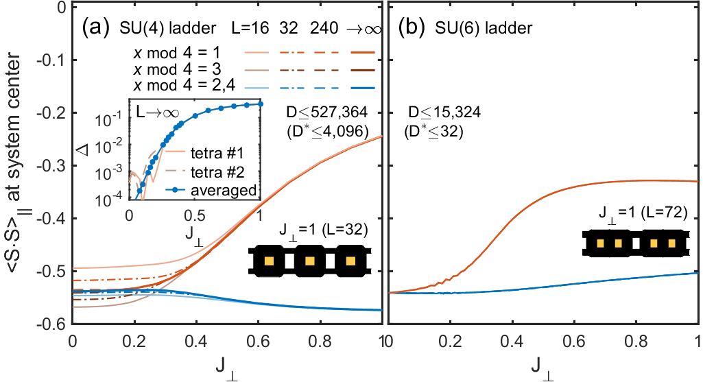
Figure 2: (Color online) $\mathrm{SU}(N)$ DMRG results for the nearest-neighbor spin correlations $\langle S\cdot S\rangle_{\|}$ for fixed bonds along the legs as a function of $J_{\perp}$ for $N=4$ (left panel) and $N=6$ (right panel). In both cases we witness the appearance of two different sets of values due to the spontaneous formation of $2\times 2$ plaquettes for $N=4$ and $3\times 2$ plaquettes for $N=6$, as depicted in the lower right insets based on actual bond energies. Panel (a) shows dimerization (and finite-size tetramerization for $J_{\perp}\lesssim 0.5$) in uniform $\mathrm{SU}(4)$ ladders of length $L=16$, $32$, $240$, together with an extrapolation $L\to\infty$ (thick lines) using open boundaries. By grouping data at fixed bond position $x\mod{N}$, two branches emerge for larger $J_{\perp}$. Tetramerization manifests itself by the additional splitting of branches towards smaller $J_{\perp}$. It vanishes in the thermodynamic limit. The inset shows the dimerization strength $\Delta$ of the extrapolated data ($L\to\infty$), where ‘tetra #$n$’ refers to the dimerization relative to the individual tetramerized branches $n=1,2$. The analysis for the $\mathrm{SU}(6)$ ladder in panel (b) is analogous to panel (a), yet takes data from a single DMRG scan [cf. App. A] that is linear in $J_{\perp}$ over the range shown, using $L=300$. By grouping data w.r.t. $x\mod{6}$, again two branches emerge, but here due to trimerization (see inset for data on an isotropic ladder for $J_{\perp}=1$) with no indication for hexamerization.

III.1 Even $N$

Our DMRG data for $N=4$ and $N=6$ is presented in Fig. 2. It demonstrates the realization of a $4k_{F}=4\pi/N$ valence bond crystal with a $N/2\times 2$ unit cell for the entire range $J_{\perp}>0$. Exemplary bond strength data along uniform ladders is shown in the insets. For $N=4$, by inversion symmetry, the rung energies are uniform throughout the ladder, i.e. are insensitive to the dimerization. Hence the analysis focuses on the bond energies along the legs for even $N$, throughout.

For $N=4$ [Fig. 2(a)], careful finite size scaling shows that the onset of strong tetramerization for $J_{\perp}\lesssim 0.5$ seen for shorter ladders and suggested as an actual possible physical phase Lecheminant and Tsvelik (2015), does reduce to a dimerized phase in the thermodynamic limit. The dimerization strength $\Delta$, defined as the difference in consecutive $\langle S\cdot S\rangle_{\|}^{\mathrm{NN}}$ correlations along the legs, vanishes only in the limit $J_{\perp}\to 0^{+}$. As demonstrated in the center inset of Fig. 2(a), by averaging data over former tetramerized branches, $\Delta$ diminishes down to below $10^{-4}$ for $J_{\perp}<0.05$.

Similarly, our data for the $\mathrm{SU}(6)$ ladder in Fig. 2(b) also supports a single symmetry broken VBC phase. Here a trimerized phase emerges in the entire antiferromagnetic regime of positive $J_{\perp}$ (see inset). Given the exponential increase in multiplet size with increasing $N$ [Weichselbaum, 2012; *Li13; *Liu15], however, a full scale DMRG simulation for $\mathrm{SU}(6)$ remained too costly. Therefore the data for smaller $J_{\perp}$ needs to be interpreted more cautiously. Nevertheless, for larger $J_{\perp}$ converged data can already be obtained with modest effort ($D^{\ast}>160$ multiplets, corresponding to $D>87,000$ states, as used for the uniform ladder in the inset to the panel).

The cases $N=4$ and $N=6$ are thus rather simple in terms of their phase diagrams, with a single VBC phase spanning the entire $J_{\perp}>0$ range, analogous to the well studied $N=2$ case where the nondegenerate rung singlet phase extends over the same parameter range. It would be interesting, but very challenging, to study even $N\geq 8$, where, as discussed previously, the large $J_{\perp}$ limit is expected to be $\mathrm{SU}(N)$₁ WZWN critical, while the weak coupling approach predicts a VBC for small $J_{\perp}$.

III.2 Odd $N$

We start with instructive data from exact diagonalization for $N=3$ shown in Fig. 3, followed by large-scale $\mathrm{SU}(N)$ DMRG data for $N=3$ and $N=5$ in Figs. 4 and 6, respectively. In the weak coupling limit, both systems demonstrate the realization of a $2k_{F}=2\pi/N$ valence bond crystal, as shown in the respective insets of Fig. 4(b) and Fig. 6(a) based on actual bond strength data. Roughly, this may be interpreted as resonating $\mathrm{SU}(N)$ singlets formed within $N\times 2$ blocks. Interestingly, for $N=3$, this VBC is consistent with the view as an extreme case of a ladder as a narrow honeycomb lattice strip where such resonating $\mathrm{SU}(3)$ singlets have been found on 6-site hexagons Corboz et al. (2013).

Both systems, $N=3$ as well as $N=5$ also have a critical phase for $J_{\perp}>J_{\perp}^{c2}$ of central charge $c=N-1$ (see App. E for excellent numerical confirmation). In between the large and small $J_{\perp}$ regime, however, we find an intermediate phase with highly non-trivial properties. These two intermediate phases differ drastically in character for $N=3$ as compared to $N=5$. We investigate the nature of the intermediate phases in more detail in the following subsections.

III.2.1 Intermediate Phase for $N=3$

From previous considerations, we understand the different phases occurring at weak $J_{\perp}$ coupling [a $N\times 2$ unit cell VBC] and at strong $J_{\perp}$ coupling [a gapless $SU(N)_{1}$ WZWN regime]. An earlier numerical and field theoretical study Corboz et al. (2007), focussing on a $J_{1}{-}J_{2}$ $\mathrm{SU}(3)$ chain, found a direct continuous transition between a $SU(3)_{1}$ WZWN regime and a trimerized VBC phase. One is led to wonder whether this scenario is also realized here in the ladder context, since the translation symmetry breaking aspects of the chain and the ladder VBCs seem related.

A closer inspection, however, reveals that this is not the case for our ladder system, and the exchange symmetry between the two legs of the ladder is responsible for the discrepancy. In the large $J_{\perp}$ limit every rung is in the antisymmetric two-box $\mathrm{SU}(N)$ irreducible representation ( ${\tiny\yng(1,1)}$ ). But these rung states are simultaneously also eigenstates of the spatial leg exchange symmetry ($\ell=1\leftrightarrow 2$) with an eigenvalue $-1$. On the other hand if one inspects the leg exchange symmetry property of an isolated open-boundary $N\times 2$ ladder block with $N$ odd at small $J_{\perp}>0$ (as a VBC cartoon state), one obtains an eigenvalue $+1$, i.e. a leg-exchange symmetric ground state. In an even further simplified representation  we can depict an $N=3$ or $N=5$ VBC unit cell as a ‘product’ state with a [ASA] ($N=3$) or [AASAA] ($N=5$) rung parity pattern, where A (S) stands for an antisymmetric (symmetric) rung multiplet. In this cartoon picture, the total leg exchange eigenvalue is given as the product over all individual rung parity eigenvalues, and hence changes sign as $J_{\perp}$ is lowered starting from large values. Note that this cartoon picture is, in fact, also reflected to some degree in the actual DMRG data for intermediate $J_{\perp}<J_{\perp}^{c1}$, e.g. see rung bond strengths in lower left inset of Fig. 6(a).

The advocated change in the spatial symmetry properties as a function of $J_{\perp}$ is a strong indication that the symmetric rung multiplets have to be taken into account in the ensuing discussion, while the single chain scenario mentioned above would be restricted to the sector where all rung multiplets remain antisymmetric ([AAA] / [AAAAA]).

It is instructive to rewrite the spin ladder Hamiltonian (2) in the rung eigenbasis, in analogy to the bond operator formulation developed originally in Ref. Sachdev and Bhatt (1990) for the $\mathrm{SU}(2)$ case. In this basis, the rung part of the Hamiltonian is diagonal and can be brought into a suggestive form,

$$J_{\perp}\sum_{x,A}S^{A}_{1,x}S^{A}_{2,x} = J_{\perp}\underset{\equiv N_{\mathrm{S}}}{\underbrace{\sum_{x}n_{\mathrm{S}}(x)}}+\mathrm{const.\ ,}$$ (18)

with $n_{\mathrm{S}}$ denoting the projector on the symmetric rung multiplet [cf. Eq. (4)], and therefore $\langle n_{\mathrm{S}}(x)\rangle$ the probability, and hence the density of a symmetric rung multiplet on the rung at position $x$. Consequently, the operator $N_{\mathrm{S}}$ counts the total number of rungs in the symmetric multiplet. This particular form thus translates the $J_{\perp}$ coupling into an effective “chemical potential” $\mu_{S}\equiv-J_{\perp}$ for the symmetric rung multiplets with the hardcore constraint of $\langle n_{\mathrm{S}}\rangle\leq 1$ symmetric multiplets per rung.

The part of the Hamiltonian involving the leg couplings $J_{\|}$ is more complicated and we refrain from providing the complete expression here. Note, however, that the total Hamiltonian conserves the parity of the number of symmetric rung states. This implies that $\langle(-1)^{N_{\mathrm{S}}}\rangle$ is quantized to $\pm 1$ but $\langle N_{\mathrm{S}}\rangle$ itself is not quantized. Still, we can approximately interpret our numerical results as though not only the parity of $N_{\mathrm{S}}$ is conserved, but even $N_{\mathrm{S}}$ itself. As discussed further below, we can indeed count the number $m$ of changes of $\langle(-1)^{N_{\mathrm{S}}}\rangle$ in the ground state as a function of $J_{\perp}$ (starting at large $J_{\perp}$) and loosely relate $\langle N_{\mathrm{S}}\rangle\sim m$. Hence the symmetric states on rungs behave like effective particles.

We now see a picture emerging where the large $J_{\perp}$ limit is characterized by the absence of symmetric rung multiplets in the ground state wave function, because the chemical potential for the symmetric rung states is exceedingly large and negative. Upon lowering $J_{\perp}$, i.e. increasing $\mu_{S}$, it might happen that at one point the lowest excitation in the other parity sector crosses the current ground state sector. Since this changes the total rung parity, this can lead to various possible phase transition scenarios, for example a Lifshitz transition where the ground state is populated by more and more symmetric rung states at the expense of antisymmetric rung eigenstates, leading to a novel $\mathrm{SU}(N)$ liquid phase with $J_{\perp}$-dependent incommensurate correlations. Another scenario would be a direct first order transition between the large $J_{\perp}$ critical regime and the VBC at weak coupling. The VBC can actually also be seen as a ”charge density wave” (CDW) of symmetric rung multiplets with a finite density $1/N$ of the rungs in the symmetric state. The question of the nature of the phase diagram in the intermediate coupling range is thus rephrased into the question of how the symmetric rung multiplets start to populate the ladder and ultimately form a period-$N$ CDW yielding the $2k_{F}$ VBC. The complementary picture starts with the CDW/VBC and asks how defects in the form of reducing $N_{\mathrm{S}}$ achieve to melt the CDW/VBC.

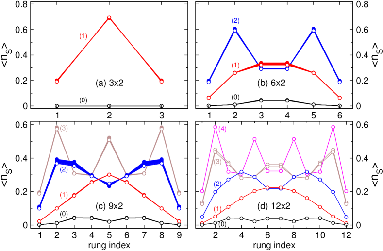
Figure 3: (Color online) $\mathrm{SU}(3)$ Heisenberg ladder — ED results showing the local rung parity for small ladders with OBC. $J_{\perp}$ varies from $1.35$ to $1.60$ in steps of $0.01$ for panels (a) to (c) and in steps of 0.05 for panel (d). The color code groups the $J_{\perp}$ values with similar profiles $\langle n_{\mathrm{S}}(x)\rangle$ [the $J_{\perp}$ values where these profiles switch are summarized in Fig. B.1]. The number $(m)$ indicates the number of significant local maxima, and coincides with the number of ground state level crossings encountered, starting with $m=0$ when coming from large $J_{\perp}$ (see main text).

Figure 4: (Color online) $\mathrm{SU}(3)$ Heisenberg ladder — Panel (a) Bond energies $\langle S\cdot S\rangle_{\|}$ vs. $J_{\perp}$ along the legs in the center of uniform systems (the analysis is completely analogous to Fig. 2 except that data is grouped w.r.t. $x\mod 3$; see legend). Within the incommensurate phase $J_{\perp}\in[{\sim 1},1.562]$ (shaded area) the bond energies vs. $J_{\perp}$ become irregular. Inset visualizes the bond energies in the center of a uniform $L=300$ ladder at $J_{\perp}=1$ (in the VBC phase). Panel (b) Bond strengths $\langle S\cdot S\rangle_{\perp}$ along the rungs [identical analysis as in (a) otherwise]. Inset shows a polynomial extrapolation of $J_{\perp}^{c1}(L)$ in the thermodynamic limit, suggesting $J_{\perp}^{c1}(L\to\infty)\sim 1$. Panel (c) Norm-squared (arb. units) of the Fourier transform of $\langle S\cdot S\rangle_{\perp}$ along uniforms ladders vs. $J_{\perp}$. The peaks related to the incommensurate wave vector $q(J_{\perp})$ are tracked by red dots [see also Fig. C.2]. Additional maxima appear at $k=\pm 2\pi/3$ (horizontal black dashed lines) that indicate the superimposed 3-rung periodicity. The vertical dashed line marks $J_{\perp}^{c2}$. Panel (d) Ground state parity $P(L)$ vs. ladder length $L=3p$ with integer $p$, superimposed with scaled nearest-neighbor $\langle S\cdot S\rangle_{\|}(x)$ data along the legs (blue) and rungs (orange), all at fixed $J_{\perp}=1.4$. For further details, see also Fig. C.4.

In order to corroborate these qualitative arguments we resort to an exact diagonalization study of open boundary $L\times 2$ ladders for a range of $J_{\perp}$ values between $1.35$ and $1.6$. In Fig. 3 we display the local rung density $\langle n_{\mathrm{S}}\rangle$ in the symmetric state as a function of the rung location $x$ for various $J_{\perp}$ values and $L=3,6,9,12$ (different subpanels). The considered $J_{\perp}$ values group into sets of curves with similar $\langle n_{\mathrm{S}}(x)\rangle$ profiles. The different sets are colored according to the number $(m)$ of significant local maxima we detect. We use this number as a proxy for the quantity $N_{\mathrm{S}}$ since, indeed, we find $\langle N_{\mathrm{S}}\rangle\sim m$. In the $L=3$ case we either find a completely vanishing curve [black, $(m=0)$], or a curve with a strong peak on the central rung [red curve, $(m=1)$]. The remaining panels present the $\langle n_{\mathrm{S}}(x)\rangle$ profiles for $L=6$, $L=9$ and $L=12$, providing further evidence for the buildup of an extended intermediate phase where the $J_{\perp}$ value controls the number of symmetric rung states $m$ and therefore the dominant spatial oscillation frequency of rung bond energies. In Fig. B.1 in App. B we display the $J_{\perp}$ values where the number $(m)$ of maxima in the $\langle n_{\mathrm{S}}(x)\rangle$ profile changes by one. These locations precisely correspond to the anticipated ground state level crossings, where the total leg-exchange parity eigenvalue alternates between $+1\leftrightarrow-1$.

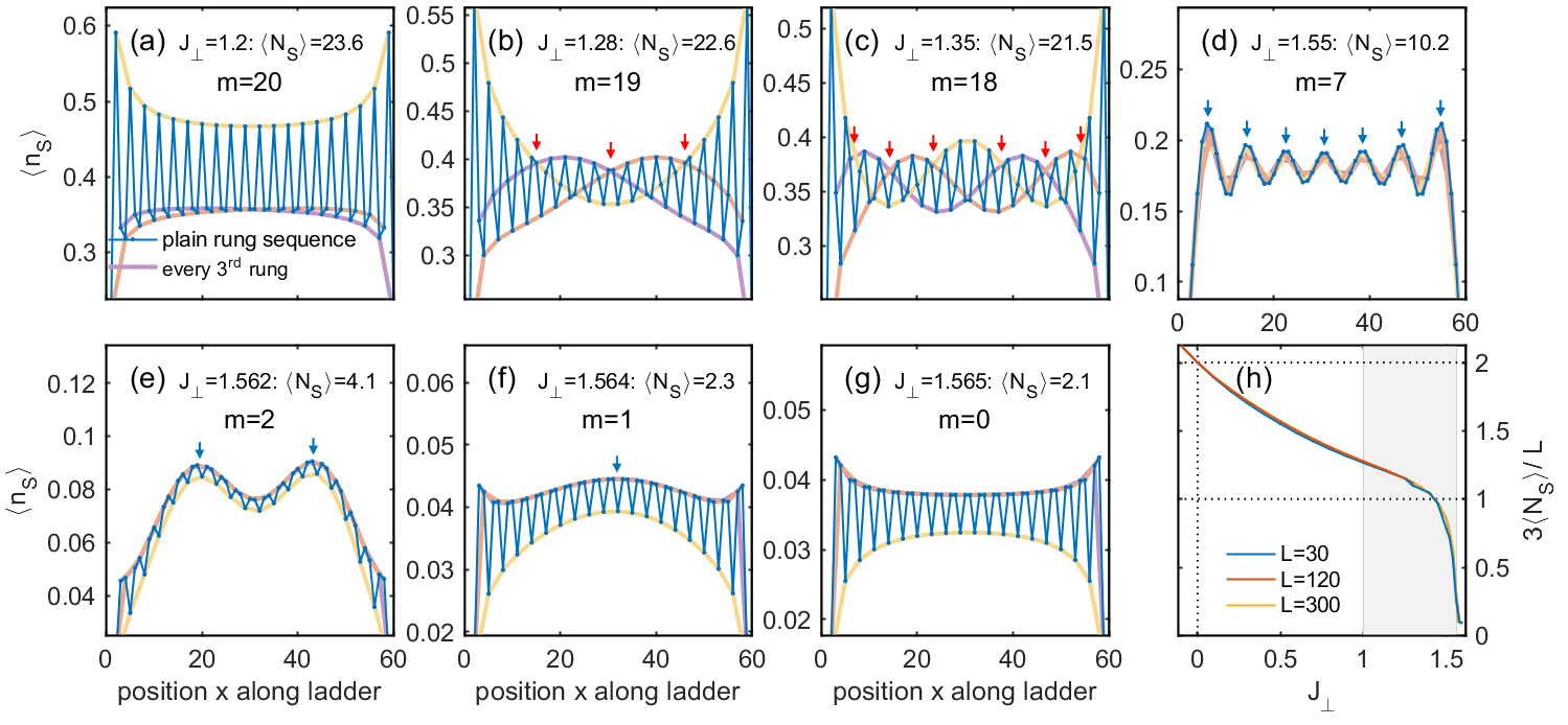
Figure 5: (Color online) Incommensurate profiles in the $\mathrm{SU}(3)$ Heisenberg ladder at length $L=60$, using $\langle n_{\mathrm{S}}\rangle=\langle S\cdot S\rangle_{\perp}+\tfrac{2}{3}$ — Panels (a-g) show different snapshots across the incommensurate regime, with panel (a) already in the commensurate small-$J_{\perp}$ regime [note that $J_{\perp}^{c1}(L=60)\gtrsim 1.20$; cf. Fig. 4], whereas panel (g) is just outside $J_{\perp}^{c2}$. Small red arrows indicate “domain walls” (upper crossings amongst light-colored lines) which is useful for $J_{\perp}$ closer to $J_{\perp}^{c1}$. Conversely, small blue arrows mark local maxima in the plain data sequence (blue) which is useful for larger $J_{\perp}$. Every panel also specifies the integrated density $\langle N_{\mathrm{S}}\rangle$ of symmetric rung multiplets. Panel (h) summarizes $\langle N_{\mathrm{S}}\rangle$ vs. $J_{\perp}$ over the full incommensurate range (shaded area) down to $J_{\perp}=0$.

With these small system exact diagonalizations in mind, we now switch to a large-scale DMRG study of the physics from weak to strong $J_{\perp}$ coupling, as summarized in Fig. 4. We first report the $J_{\perp}$ dependence of the nearest-neighbor spin-spin correlations in the center of systems as large as $L=300$ along the legs and rungs in Fig. 4(a) and (b), respectively. We can distinguish three regions. The small $J_{\perp}$ regime extending from $0^{+}$ to about $J_{\perp}\sim 1\equiv J_{\perp}^{c1}$ represents the $2k_{F}$ VBC. The large $J_{\perp}$ regime $J_{\perp}>1.562\equiv J_{\perp}^{c2}$ describes the gapless $SU(3)_{1}$ WZWN phase. These two phases are separated by the intermediate phase with $J_{\perp}\in[J_{\perp}^{c1},J_{\perp}^{c2}]$ [shaded areas in Fig. 4(a-b)] which corresponds to a gapless incommensurate phase, as qualitatively suggested by the preceding discussion.

The incommensurate behavior of the system is analyzed in Fig. 4(c) via spatial Fourier transform in the leg direction of the rung bond strengths $\langle S\cdot S\rangle_{\perp}$. The incommensurate wavevector $q(J_{\perp})$ is determined by local maxima as traced by the red dots, which are further analyzed in Fig. C.2.

The upper boundary $J_{\perp}^{c2}$ is extremely steady and easily visible already within exact diagonalization of very small system sizes, resulting in $J_{\perp}^{c2}\approx 1.56$, [see App. B.1]. From DMRG simulations for $L=60$ ladders, the value is $J_{\perp}^{c2}=1.562$ to within an uncertainty of $+0.002$ towards a slightly larger value. The sharpness of the upper boundary $J_{\perp}^{c2}$ is due to vertical slope in the incommensurate wavelength in Fig. 4(c), $\bigl{|}\tfrac{dq}{dJ_{\perp}}\bigr{|}_{(J_{\perp}^{c2})^{-}}\to\infty$. In contrast, the lower boundary $J_{\perp}^{c1}$ is strongly sensitive on system size, as it depends on whether or not an incommensurate wave length still fits into a given finite system. Here for $L=60$, the transition to commensuration actually already occurs around $J_{\perp}\sim 1.2$ [Fig. 4(c)]. For significantly larger systems this moves as low as $J_{\perp}\simeq 1.08$ (data not shown). In this sense, $J_{\perp}^{c1}\approx 1$ is an estimate from an extrapolation as shown in the inset of Fig. 4(b). Now given that the slope $\tfrac{dq}{dJ_{\perp}}$ tends to zero for $J_{\perp}\to(J_{\perp}^{c1})^{+}$, one may question whether a finite $J_{\perp}^{c1}>0$ exists at all. However, this transition at a finite $J_{\perp}^{c1}$ is confirmed in Fig. C.3. There we show that the $\mathrm{SU}(3)$ ladder is gapped e.g. at $J_{\perp}=0.75$ in the thermodynamic limit and that, indeed, this gap closes around $J_{\perp}\sim 1$.

The incommensurate behavior of the bond energies is tightly linked to the global ground state parity $P$ as $L$ is varied. As demonstrated in Fig. 4(d), for every full incommensurate period $\lambda/2$ [cf. Fig. C.4] in the bond energies along a single long ladder, also the parity of the ground state of a short ladder flips when changing its length $L\to L+\lambda/2$ (black data). This confirms the intuitive notion that by hosting a symmetric rung state, this replaces an antisymmetric rung state, and hence changes the parity. As an aside, Fig. 4(d) also shows that the incommensurate behavior on bond energies along rungs completely coincides with an incommensurate behavior also seen for the bond energies along the legs.

Next we revisit the ED analysis of the $\langle n_{\mathrm{S}}(x)\rangle$ profiles in Fig. 3, but now for significantly larger system at $L=60$ based on DMRG data. With $\langle n_{\mathrm{S}}\rangle=\langle S\cdot S\rangle_{\perp}+\tfrac{2}{3}$ [cf. Eq. (4)], this further analyzes the data underlying Fig. 4(b-d). The DMRG data is presented in Fig. 5 for various values of $J_{\perp}$. In each panel (a-g) we draw the bare data (blue line), but also draw additional lines by connecting every third data point to better visualize the incommensurate behavior, using different lighter colors for different values of (${x}{\mod 3}$). Panel (a) is just below $J_{\perp}^{c1}(L=60)$, having $J_{\perp}=1.2$, whereas panel (g) is just above $J_{\perp}^{c2}$.

Figure 5(h) summarizes the actual expectation values $\langle N_{\mathrm{S}}\rangle$ vs. $J_{\perp}$, where the data plotted, $\langle\nu_{\mathrm{S}}\rangle\equiv 3\langle N_{\mathrm{S}}\rangle/L$, corresponds to the density of symmetric rung states per $3$ rungs. Note that at the boundaries of the incommensurate phase (shaded area) $\langle\nu_{\mathrm{S}}\rangle$ is not strictly integer. For example, just above $J_{\perp}^{c2}$, $\langle\nu_{\mathrm{S}}\rangle\simeq 0.1$ is finite due to presence of virtual excitations into the symmetric multiplet at higher energies. Just below $J_{\perp}^{c1}$, $\langle\nu_{\mathrm{S}}\rangle\simeq 1.27$ is somewhat above $1$ for the same reason. In this sense, as already pointed out in the ED discussion earlier, the equivalence of $\langle N_{\mathrm{S}}\rangle$ and $m$ is not strict because $\langle N_{\mathrm{S}}\rangle$ also contains an inseparable contribution from virtual excitations. Note that $\langle\nu_{\mathrm{S}}\rangle$ is also not constant within the VBC phase, since for $J_{\perp}<J_{\perp}^{c1}$, $\langle\nu_{\mathrm{S}}\rangle$ necessarily increases still up to $\langle\nu_{\mathrm{S}}\rangle=2$ at $J_{\perp}=0$ which, matter of fact, is the expected value for two decoupled chains. Within the incommensurate region, however, $\langle N_{\mathrm{S}}\rangle$ closely follows the dependence of $m$. The switching of the ground state parity vs. $J_{\perp}$ for fixed system length $L$, on the other hand, is an exactly countable feature within the numerical simulations [e.g. see also Fig. C.4(b)], which thus makes $m$ a well-defined quantized integer.

Figure 5(a) shows the CDW/VBC with a regular period 3 pattern. It has $m=L/3=20$ ($\langle N_{\mathrm{S}}\rangle=23.6$). Here, due to finite size, the system is already locked into the VBC phase. At the other end of the incommensurate regime, panel (f) already belongs to the large $J_{\perp}$ regime with $m=0$ ($\langle N_{\mathrm{S}}\rangle=2.1$). The small oscillations visible in panel (g) are an order of magnitude smaller than in the VBC phase [panel (a)], and in contrast to VBC phase, they decay with system size. When the ground state switches from the $\langle n_{\mathrm{S}}(x)\rangle$ profile in Fig. 5(g) down to the panels (f) and (e), with each switch the expectation value $\langle N_{\mathrm{S}}\rangle$ increases by approximately 1, having $m=0,1,2$, respectively, as indicated by $m$ blue arrows [the case $m=1$ in panel (f) is very close to the phase boundary $J_{\perp}^{c2}$ hence its value of $\langle N_{\mathrm{S}}\rangle$ is strongly affected by the finite system size]. Figure 5(d) already reaches $m=7$.

Figure 5(c) down to (a) correspond to $m=18,19$, and $20$, respectively. Here it is more challenging to identify the location of these $m$ symmetric rung states. However one can spot the appearance of $3\times(L/3-m)$ domain walls between different local patterns of the three degenerate CDW/VBC patterns Su and Schrieffer (1981) whose positions are indicated by the red arrows. These 3 or 6 domain walls in Fig. 5(b) or (c), respectively, are fractionalized defects introduced into the CDW/VBC by reducing $\langle N_{\mathrm{S}}\rangle$ by approximately 1 for each switch in the $\langle n_{\mathrm{S}}(x)\rangle$ profile when going from Figure 5(a) to (b), or from (b) to (c). It thus seems that one symmetric rung state defect doped into the CDW/VBC decays into three domain walls, a hallmark of fractionalization Su and Schrieffer (1981).

In summary, the incommensurate wave length tracked by the red dots in Fig. 4(c) can be rationalized as $q(J_{\perp})=\pm\tfrac{2\pi}{L}m(J_{\perp})$, where the integer $m$ $(\sim{\langle N_{\mathrm{S}}\rangle})$ denotes e.g. the number of level crossings discussed above. Figure 4(c) highlights the Lifshitz-like transition occurring at $J_{\perp}^{c2}$, when the first symmetric rung states start to populate the ladder upon lowering $J_{\perp}$. In the intermediate phase, $J_{\perp}$ controls the incommensuration in a way reminiscent of magnetization curves in the vicinity of magnetization plateaux or the density controlled by a chemical potential in the vicinity of a quadratic band edge. The difficulty in precisely locating the lower boundary of the incommensurate gapless phase seems to be tied to the nature of the period-3 CDW/VBC which neighbors the incommensurate phase. It has been observed in a number of one-dimensional CDW-like systems, that the doping of the CDW can lead to a fractionalization of the defects, leading to a seemingly slow onset of the incommensuration with the field or chemical potential, see e.g. Refs. Yang and Yang (1966); Okunishi and Tonegawa (2003); Fouet et al. (2006a).

III.2.2 Intermediate Phase for $N=5$

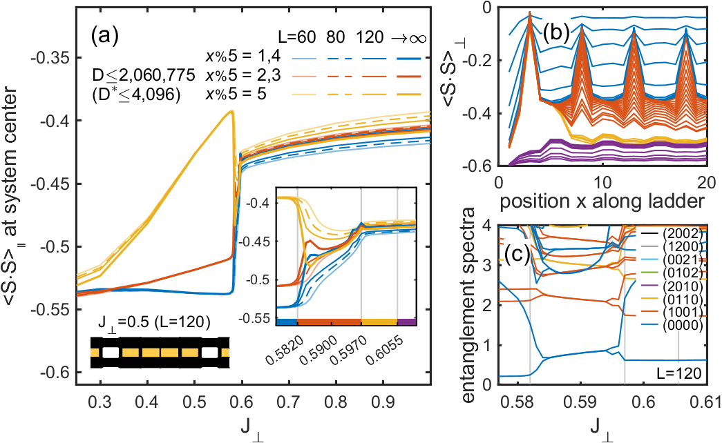
Figure 6: (Color online) $\mathrm{SU}(5)$ Heisenberg ladder — Panel (a) Similar analysis as in Fig. 2(a), yet grouping data w.r.t. $x\mod 5$ (see legend). This results in three branches for $J_{\perp}<0.581\equiv J_{\perp}^{c1}$ due to pentamerization, as shown in the lower left inset for $J_{\perp}=0.5$. From our numerical data we conclude that this gapped phase persists down to $J_{\perp}\to 0^{+}$. The lower right inset shows a zoom into the extremely narrow intermediate phase for $J_{\perp}\in[0.581,0.596]$. Panel (b) Nearest-neighbor $\langle S\cdot S\rangle_{\perp}^{\mathrm{NN}}$ rung data at the open left boundary of the system. By color coding the ranges in $J_{\perp}$ as with the x-axis in the lower right inset of panel (a), the intermediate phase is linked to the sharp emergence of an edge feature at the open boundary of the ladder. Panel (c) Analysis of the entanglement flow for the same window in $J_{\perp}$ as the right inset in (a). These entanglement spectra were computed for fixed $J_{\perp}$ in the center of uniform length $L=120$ ladders Lines with the same color belong to the same $\mathrm{SU}(5)$ symmetry sector, using a compact Dynkin labeling scheme in the legend (see App. A). The results are also consistent with DMRG scans in $J_{\perp}$ (e.g. see Fig. D.5 in App. D).

The same symmetry considerations regarding the rung parity change coming from the large $J_{\perp}$ regime to the small $J_{\perp}$ VBC regime apply to $N=5$. Whereas in the $N=3$ case this change occurs gradually in a rather extended $J_{\perp}$ region, the case $N=5$ is quite different. At first sight the transition seems to happen quite abruptly around $J_{\perp}\sim 0.58$, however a careful DMRG investigation shows that the critical, large $J_{\perp}$ and the small $J_{\perp}$ VBC phases are separated by a finite (albeit rather tiny) intermediate phase, thus avoiding a direct first order transition. We present a compact overview of these findings in this subsection and provide in-depth material in App. D.

Our results for the $\mathrm{SU}(5)$ ladder are summarized in Fig. 6. It features an extremely narrow intermediate phase that stretches over a less than 3% variation of $J_{\perp}\in[0.581,0.596]$. Yet it is stable, in the sense that its window slightly increases with increasing system size [inset to Fig. 6(a)]. Importantly, it smoothly connects strongly different values of $\langle S\cdot S\rangle_{\|}$ for $J_{\perp}<J_{\perp}^{c1}$ as compared to $J_{\perp}>J_{\perp}^{c2}$. Consequently, what would have been a first order transition in the absence of the intermediate phase, become two (possibly) second-order phase transitions.

In stark contrast to the $\mathrm{SU}(3)$ case, however, the intermediate phase of the $\mathrm{SU}(5)$ ladder shows no signs of incommensuration in the nearest-neighbor spin-spin correlations [e.g. see smooth behavior of the nearest-neighbor $\langle S\cdot S\rangle$ data across entire intermediate phase in Fig. D.5(c)]. Instead, the data for the intermediate phase in Fig. 6 show properties that are typically rather associated with topological phases: (i) The multiplets in the entanglement spectra pair up extremely systematically, as shown in Fig. 6(c) [see also Fig. D.5(d)]. (ii) A striking edge feature snaps into the system when approaching the intermediate phase from large $J_{\perp}$. (iii) Finite size extrapolation in the bond strengths reduces the strength in pentamerization, which may points towards a uniform isotropic ladder in the thermodynamic limit [see inset to Fig. 6(a)].

The edge feature, as shown in Fig. 6(b), already occurs for a value of $J_{\perp}$ slightly outside $J_{\perp}^{c2}$, and therefore initially it appears as a pure boundary feature. This fact alone could be interpreted as a precursor of a first-order transition due to open boundary conditions Fouet et al. (2006b). Nevertheless, once $J_{\perp}$ crosses $J_{\perp}^{c2}$, the edge feature still persists within the intermediate phase where the bulk properties of the system change profoundly. More supporting data is also provided in App. D.

Furthermore, while the nearest-neighbor spin-spin correlations in the case of the $\mathrm{SU}(5)$ ladders are commensurate, there are traces of incommensuration, e.g. seen in the minor wiggles in the entanglement spectra in Fig. 6(c) just below $J_{\perp}^{c2}$ [with more resolution shown in Fig. D.5(d) and its inset]. This incommensuration also appears reflected e.g. in the non-local expectation values of the block-parity [Fig. D.6(a)]. Nevertheless, in either case, the incommensuration decays quickly when going into the bulk of the ladder [e.g. see Fig. D.6(b)].

A simple intuitive picture, however, that accounts for all the properties seen in this newly uncovered intermediate phase in the $\mathrm{SU}(5)$ ladders is still lacking. It shall also be noted that for Heisenberg ladders with a well-defined local multiplet, a generalized Lieb-Schultz-Mattis (LSM) theorem applies Lieb et al. (1961); Affleck and Lieb (1986); Affleck (1988b). As a consequence, our two-leg ladder in the defining representation of $\mathrm{SU}(N)$ either spontaneously breaks translation symmetry, or necessarily possesses soft modes at momentum $4\pi/N$  and hence a gapless spectrum. This is found, for instance, in the small and large $J_{\perp}$ regions for $N=3$ and $N=5$. In the intermediate phase for $N=5$, however, we clearly see a two-fold degenerate ground state and systematic two-fold degeneracy in the entanglement spectra, all of which is tightly linked to parity and thus apparently decoupled from the $\mathrm{SU}(5)$ symmetry. The two-fold degeneracy may be related to the presence of the open boundaries. A more detailed study based on periodic boundary conditions, however, is currently not feasible numerically, given that within the intermediate phase the $\mathrm{SU}(5)$ ladders up to length $L=30$ with periodic boundary conditions are still too strongly affected by finite size effects. For the same reason, even when using open boundary conditions, we cannot make definitive statements on whether or not the ground state in the $\mathrm{SU}(5)$ intermediate phase is translationally uniform in the thermodynamic limit.

IV Conclusion and Outlook

We analyze the $\mathrm{SU}(N)$ Heisenberg ladder for antiferromagnetic $J_{\perp}$ with relevance for materials Dagotto and Rice (1996); Caron et al. (2011); Luo et al. (2013); Schmidiger et al. (2013) as well as experiments in ultracold atoms Jördens et al. (2008); Lake et al. (2010); Ward et al. (2013); Cazalilla and Rey (2014); Zhang et al. (2014); Scazza et al. (2014); Cappellini et al. (2014); Pagano et al. (2014); Hofrichter et al. (2016). We uncover rich phase diagrams that strongly depend on the parity of $N$. For even $N\leq 6$, the spectrum is always gapped and the ground state is a $4k_{F}$ VBC. For odd $N$, we find a $2k_{F}$ gapped VBC phase at weak coupling, a critical phase at strong coupling, and an intermediate phase that is incommensurate for $N=3$, but extremely narrow and reminiscent of topological phases for $N=5$. While topological phases of the type encountered can be ruled out for a single chain Duivenvoorden and Quella (2013); Capponi et al. (2016), it is emphasized that the present system of a 2-leg ladder has an additional discrete parity symmetry that is playing an essential role.

We focused on the Mott insulating regime of symmetric multi-flavor fermionic Hubbard models at filling of one particle per site. Our detailed analysis vs. the number of flavors $N$ already uncovers a remarkable phase diagram, which reflects the complexity of strongly-correlated quantum many-body phenomena, in general. The full exploration of the original fermionic Hubbard model for $N>2$ flavors, however, e.g. at different integer fillings as well as doped systems for arbitrary chemical potential and the full range of interaction strength $U$ remains a wide, largely unexplored, yet exciting open field for future research. From a different perspective, our model with strong ferromagnetic rung will map onto an effective chain with symmetric ${\tiny\yng(2)}$ irrep of $\mathrm{SU}(N)$, for which there exists a generalized Haldane conjecture Rachel et al. (2009) and recent progress was made to understand such symmetric irreps for $N=3$ Lajkó et al. (2017). More generally, larger representations are a simple way to stabilize more exotic phases such as chiral ones Hermele and Gurarie (2011). Another direct extension of this work would be to study similar geometries such as zigzag ladders, which can be realized experimentally Anisimovas et al. (2016) where frustration is expected to play an important role. By focusing on symmetric models, however, the full exploitation of the underlying non-abelian symmetries offers the prospect of a significant advance in terms of exact numerical simulations on these systems.

Appendix A DMRG simulations of SU(N) ladders

The DMRG White (1992); Schollwöck (2005, 2011) data in the main text as well as in these appendices fully exploit the underlying $\mathrm{SU}(N)$ symmetry based on the QSpace tensor library Weichselbaum (2012). While QSpace can deal with general non-abelian symmetries, the discussion in the following is constrained to $\mathrm{SU}(N)$. By operating on the level of irreducible representations (ireps) rather than individual states, by construction, symmetry multiplets remain intact. Conversely, from a practical point of view, by switching from a state-spaced description to a multiplet based description, e.g. for the case of $\mathrm{SU}(5)$, this allows us to effectively keep beyond a million of states, and therefore to go significantly beyond the current state-of-the-art of DMRG simulations.

A ladder of length $L$ is represented by an $2\times L$ lattice, and hence consists of $L$ rungs and $2L$ sites. The DMRG simulation proceeds along a snake-like pattern from rung to rung, and therefore operators on a chain of $2L$ sites. While this makes the algorithm more efficient, this does not explicitly include the parity symmetry w.r.t. exchange of upper and lower leg. Throughout we use the term parity symmetry to refer to this reflection symmetry, nevertheless. All energies are taken in units of $J_{||}:=1$, with $J_{\perp}\geq 0$.

DMRG simulations can also be used to scan parameter regimes by (slowly) tuning parameters in the Hamiltonian (here $J_{\perp}$) e.g. as a linear function of the ladder position $x$ within a single DMRG runZhu and White (2015). This is referred to as a DMRG scan. In the resulting plots we directly show the underlying tuned parameter $J_{\perp}$ rather than the ladder position $x$. To be explicit, we may also may write the label of the horizontal figure axis e.g. as “position $x$ along the ladder $\to J_{\perp}$”. These scans serve the purpose of quick snapshots of the physical low-energy behavior along a line in parameter space with blurred open boundary condition. Eventually, these calculations are typically followed by DMRG simulations of uniform systems at specific parameter points of interest.

Symmetry labels for $\mathrm{SU}(N)$ multiplets are specified by their Dynkin labels $q\equiv(q_{1},\ldots,q_{\mathpzc{r}})$, with $\mathpzc{r}=N-1$ the rank of the symmetry $\mathrm{SU}(N)$ and $q_{i}\in\mathbb{N}_{0}$ non-negative integers Elliott and Dawber (1979); Gilmore (2006); Weichselbaum (2012). For example, the Dynkin label for an $\mathrm{SU}(2)$ multiplet of spin $S$ is given by $q=(q_{1})$, with $q_{1}=2S$ the number of boxes in its Young tableau. For general $\mathrm{SU}(N)$, the Dynkin labels count the differences from one row of a Young tableaux to the next, with the total number of boxes in the corresponding Young tableau $Y_{q}$ given by $n_{Y}\equiv\sum_{k=1}^{N-1}k\cdot q_{i}$.

Throughout, a compact label format is adopted that simply skips commata and spaces in a set of Dynkin labels. For example, $(10)\equiv(1,0)$ is the defining representation of $\mathrm{SU}(3)$ of dimension $d=3$. If the labels $q_{i}$ have values beyond $9$, the counting is continued with alphabetic characters $A-Z$ [e.g. $(1A)\equiv(1,10)$ akin to hexadecimal digits]. This suffices for all practical purposes since no labels with values $q_{i}>Z\equiv 35$ are encountered.

When convenient and unique, the alternative convention of specifying a multiplet simply by its dimension ${\bf d}$ is adopted. For example, for $\mathrm{SU}(3)$ the defining representation is given by $\mathbf{3}\equiv(10)$. This customary labeling scheme becomes ambiguous, though, and thus fails if different non-dual multiplets share the same multiplet dimension [e.g. for $\mathrm{SU}(3)$, the ireps (40) and (21) have the same dimension $d=15$]. The labeling scheme by dimension (as far as applicable) uses bold font to emphasize that a multiplet typically represents multiple symmetric states. These multiplets can quickly become “fat” for larger $\mathrm{SU}(N)$. In practice, they quickly reach dimensions up to $d\lesssim 10^{\mathpzc{r}}$, again with $\mathpzc{r}=N-1$ the rank of the symmetry $\mathrm{SU}(N)$. That is while $\mathrm{SU}(2)$ typical encounters multiplets that only have up to $\lesssim 10$ states (i.e. spin $S\lesssim 5$), for $\mathrm{SU}(5)$, in fact, this quickly reaches up to and beyond $d=10,000$ states for a single multiplet!

The dual or “barred”-representation $\bar{q}$ always shares exactly the same dimension $d=|q|$ in terms of number of states as the original irep $q$. In Dynkin labels, the dual irep in $\mathrm{SU}(N)$ is simply given by reversed labels, i.e. $\bar{q}=(q_{N-1},\ldots,q_{1})$. For example, the dual to the defining irep is given by $\bar{\bf N}\equiv(0\ldots 01)$. While $|\bar{{\bf d}}|=|{\bf d}|$, by convention, $\bar{{\bf d}}\leq{\bf d}$ in lexicographic order on their corresponding Dynkin labels, where equality holds for self-dual ireps.

The spin operator always transforms in the adjoint representation of dimension $d=N^{2}-1$ which simply represents the set of all generators of the Lie algebra. It is obtained whenever a non-scalar multiplet $q$ is combined with its dual $\bar{q}$. For example, taking the defining representation, ${\bf N}\otimes\bar{\bf N}\equiv(10\ldots 0)\otimes(0\ldots 01)=1+(10\ldots 01)$, with $1\equiv(0\ldots 0)$ the scalar representation, one arrives at the symmetry labels of the spin operator for $\mathrm{SU}(N>2)$, given by $q_{S}=(10\ldots 01)$. For $\mathrm{SU}(2)$, one has $(1)\otimes(1)=(0)+(2)$ and therefore $q_{S}=(2)$, i.e. $S=1$.

Even though we consider general $\mathrm{SU}(N)$ symmetries, we will nevertheless use the familiar $\mathrm{SU}(2)$ language where convenient and possible. That is, the $\mathrm{SU}(2)$ spin operator $\hat{\mathbf{S}}$ is generalized to the $\mathrm{SU}(N)$ “spin” operator where $\hat{S}^{A}$ are the $\mathrm{SU}(N)$ spinor components with $A=1,\ldots,N^{2}-1$, e.g. as used in Eq. (2) or Eq. (6) in the main text. In particular, we also refer to $S\cdot S$ as the (generalized) spin-spin interactions. For example, $\langle S\cdot S\rangle_{\|}$ will refer to the nearest-neighbor $S\cdot S$ expectation values along the legs in the DMRG ground state $|0\rangle$, i.e.

$$\langle S\cdot S\rangle_{\|} \equiv \langle 0|\hat{\mathbf{S}}_{\ell x}\cdot\hat{\mathbf{S}}_{\ell,x+1}|0\rangle\equiv\sum_{A}\langle 0|\hat{S}^{A}_{\ell x}\,\hat{S}^{A}_{\ell,x+1}|0\rangle\text{,}\ \ \qquad$$ (19)

For the $\mathrm{SU}(N)$ ladder systems considered here, these expectation values along the legs are always the same for either of the two legs $\ell=1,2$ (“upper” and “lower” leg), hence the leg-index $\ell$ can be dropped [i.e. without implicit summation over $\ell$ in Eq. (19)]. The index $x$, finally, refers to the position along the ladder with lattice spacing $a=1$. Hence $x\pm 1$ refers to nearest neighbor rungs. Depending on the context, $x$ may also refer to the bond in between rungs $x$ and $x+1$.

Similarly, $\langle S\cdot S\rangle_{\perp}$ refers to nearest-neighbor spin correlators across a single rung, i.e.

$$\langle S\cdot S\rangle_{\perp} \equiv \langle 0|\hat{\mathbf{S}}_{1x}\cdot\hat{\mathbf{S}}_{2x}|0\rangle\equiv\sum_{A}\langle 0|\hat{S}^{A}_{1x}\,\hat{S}^{A}_{2x}|0\rangle\text{.}\ \ \qquad$$ (20)

In general, $\langle S\cdot S\rangle_{\|}$ and $\langle S\cdot S\rangle_{\perp}$ depend on the position $x$.

The Heisenberg ladders under consideration have the defining irep at each site. For this specific case, the scalar operators $\mathbf{S}_{i}\cdot\mathbf{S}_{j}$ acting e.g. on nearest-neighbor sites $i\equiv(\ell x)$ and $j\equiv(\ell^{\prime}x^{\prime})$ can be simply related to the parity $\hat{P}_{i,j}$ which swaps the states of the two sites. In particular then, it holds for general $\mathrm{SU}(N)$ for two sites $i\neq j$,

$$\hat{P}_{ij}=\tfrac{1}{N}+2\,\mathbf{S}_{i}\cdot\mathbf{S}_{j}\text{ .}$$ (21)

This can be derived from elementary symmetry considerations as follows. Given that we only consider the defining representation $q$ of $\mathrm{SU}(N)$ on each site, from the product $q\otimes\bar{q}$ we see that aside from the trivial identity operator $\hat{1}$, the only non-trivial operators that can act on the state space of a single site $i$ are the components of the spin operator $\hat{\mathbf{S}}_{i}$. Consequently, the only non-trivial scalar operator that can act across two sites $i$ and $j$ as part of an interaction term in a Hamiltonian is the spin-spin interaction $\mathbf{S}_{i}\cdot\mathbf{S}_{j}$. On the other hand, the permutation $\hat{P}_{ij}$ (i.e. swap) of two sites $i$ and $j$ is also a non-trivial hermitian operator that can equally well serve as an individual term in an $\mathrm{SU}(N)$ symmetric Hamiltonian. From the above elementary symmetry considerations, therefore it follows that $\hat{P}_{ij}$ must be a combination of the trivial operator and spin interaction, i.e. $\hat{P}_{ij}=a\,\hat{1}_{ij}+b\,\mathbf{S}_{i}\cdot\mathbf{S}_{j}$, with coefficients $a$ and $b$ to be determined. Clearly, with the spin operators being traceless, then with the normalization convention $\mathrm{Tr}(S_{i}^{A}S_{i}^{B})=\tfrac{1}{2}\delta_{AB}$ [cf. Eq. (6)], it must hold within the state space of two defining representations of $\mathrm{SU}(N)$ at sites $i$ and $j$ that $N=\mathrm{Tr}(\hat{P}_{ij})=aN^{2}$, and hence $a=\tfrac{1}{N}$. Furthermore, with $\hat{P}_{ij}^{2}=\hat{1}_{ij}$, it follows $N^{2}=\mathrm{Tr}(\hat{P}_{ij}^{2})=a^{2}\,\mathrm{Tr}(\hat{1}_{ij})+b^{2}\,\mathrm{Tr}((\mathbf{S}_{i}\cdot\mathbf{S}_{j})^{2})=1+b^{2}\,(N^{2}-1)\bigl{(}\tfrac{1}{2}\bigr{)}^{2}$, and therefore $b=2$ which proves Eq. (21).

Appendix B Further exact diagonalization results
on the $N=3$ intermediate phase

As a first attempt to check the phenomenological picture for the $N=3$ intermediate phase, namely that starting from strong coupling where the rungs are predominantly antisymmetric, we want to understand the effect of decreasing $J_{\perp}$ in terms of symmetric rung density. We have performed Exact Diagonalization (ED) using Lanczos algorithm on ladders $2\times L$ ($L$ is chosen as a multiple of 3 to accomodate a singlet state as well as the VBC expected at weak coupling) with open boundary conditions (OBC) using global color conservation. We can also use the global parity, that exchanges the two legs, as a discrete symmetry, and hence label the ground-state as even or odd.

From the strong coupling picture at large $J_{\perp}$ where all rungs are antisymmetric, it is clear that the ground-state should have parity $(-1)^{L}$. In Fig. B.1, we do confirm this statement, but we also notice that, while decreasing $J_{\perp}$, there is a sequence of level crossings: on a $2\times(3p)$ ladder, there are $p$ changes in the ground-state parity. Moreover, the range of parameters for these transitions is quite wide, in good agreement with the extension of the incommensurate phase found in DMRG simulations.

Overall, these ED data suggest that there is no sharp first order transition, but rather a finite intermediate region.

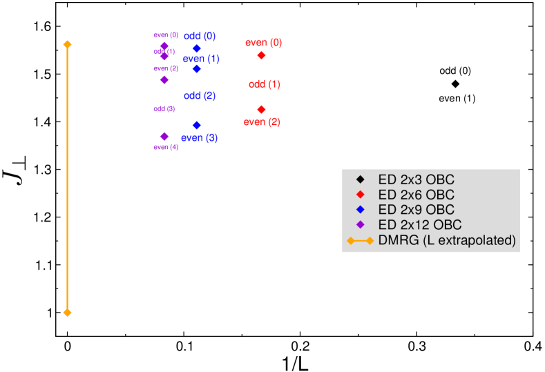
Figure B.1: (Color online) Locations of the changes in the ground-state parity obtained from ED results on $\mathrm{SU}(3)$ Heisenberg $2\times L$ ladder as a function of $1/L$. The number $(N_{\mathrm{S}})$ indicates the number of ground state level crossings encountered coming from large $J_{\perp}$ (see Fig. 3 in the main text). There are $L/3$ level crossings distributed over a significant region of $J_{\perp}$, compatible with the extension of the intermediate phase found in DMRG.

Appendix C Further DMRG results
  on the $N=3$ intermediate phases

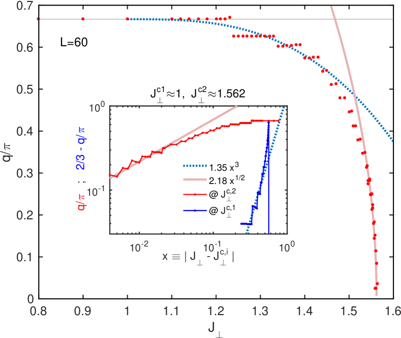
Figure C.2: (Color online) Incommensurate wave length in uniform SU(3) Heisenberg ladders of length $L=60$ with open boundaries in the incommensurate regime $J_{\perp}\in[J_{\perp}^{c1},J_{\perp}^{c2}]\equiv[{\sim}~{}1,1.562]$ [data taken from Fig. 4(c) in the main paper, where red points trace the incommensurate maxima in Fourier space]. The inset suggests a scaling for the incommensurate wave vector that is $\bigl{(}\tfrac{2\pi}{3}-q\bigr{)}\propto|J_{\perp}-J_{\perp}^{c1}|^{\sim 3}$ close to $J_{\perp}^{c1}$, and $q\propto\sqrt{|J_{\perp}-J_{\perp}^{c2}|}$ close to $J_{\perp}^{c2}$.

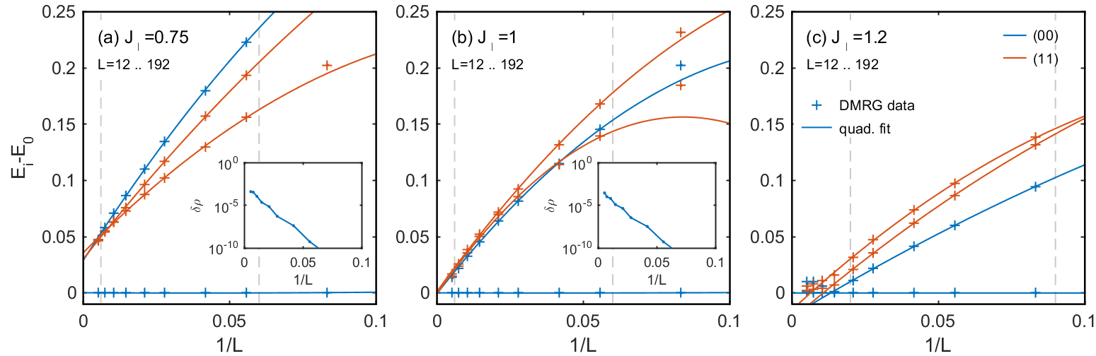
Figure C.3: Analysis of excited states across the lower boundary $J_{\perp}^{c1}$ of the incommensurate phase for the $\mathrm{SU}(3)$ Heisenberg ladder. Panel (a) for $J_{\perp}=0.75$ shows a small but finite energy gap when extrapolating to the thermodynamic limit $1/L\to 0$. Panel (b) at $J_{\perp}=1$ suggests the onset of criticality, whereas for panel (c) at $J_{\perp}=1.2$ due to the presence of incommensurate correlations other states take over the ground state for sufficiently large systems (see crossing of the lowest blue line, which served as energy reference). For the simulations here, several lowest system eigenstates are targeted simultaneously within a single DMRG run for uniform systems up to length $L=96$ using open boundary conditions. The colors encode symmetry sectors, which shows that two multiplets were included in the $q=(00)\equiv\mathbf{1}$ sector (singlets; blue data points) as well as two multiplets in the adjoint representation $q=(11)\equiv\mathbf{8}$ (orange data points). Therefore while only including $4$ multiplets total, this DMRG simulations actually targeted the lowest 18 states. The insets of panels (a-b) show the maximum discarded weight within DMRG in the last sweep while simultaneously targeting the low-energy multiplets above. For all ladders at least $1024$ multiplets ($>51,000$ states) were kept. For $L\leq 69$, at least $2048$ multiplets ($>111,000$ states) were kept. The gray vertical lines indicate the region that was used to fit the data (crosses) to the thermodynamic limit $L\to\infty$ using a plain quadratic polynomial fit (solid lines).

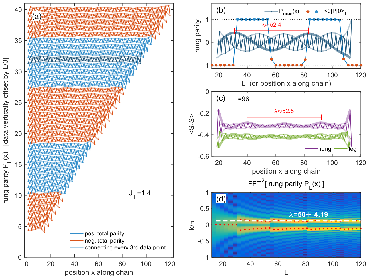
Figure C.4: Analysis of the incommensurate phase in the $\mathrm{SU}(3)$ Heisenberg ladder for $J_{\perp}=1.4$. Panel (a) shows the block parity $P_{L}(x)\in[-1,1]$ of the ground state [cf. Eq. (22)], where the data is vertically offset by the integers $L/3$ for different system sizes $L=15,18,\ldots,120$. The incommensurate wave is highlighted by simply also connecting only every third data point (light colors). The total rung parity, i.e. the last data point $P_{L}(L)$ of each curve determines whether the full ground state is symmetric (blue) or antisymmetric (orange) under rung exchange. Panel (b) compares the block parity $P_{L}(x)$ for a single system of fixed length $L=96$ [data horizontally offset by $dx=17.5$; data also marked in darker colors in (a)] to the full parity $P(L)$ for systems vs. varying length $L$ (dots) [this corresponds to the last data points $P_{L}(L)$ of each curve in (a)]. The resulting incommensurate period of $P_{L}(x)$ clearly matches the period seen in $P(L)$. For comparison, panel (c) shows the incommensurate behavior seen in the $\langle S\cdot S\rangle$ data [similar to panel (b), again for $L=96$, and data horizontally offset]. The incommensurate wave length is the same up to a factor of $2$ (see text). Panel (d) shows the Fourier transform of the data in panel (a). In order to focus on the incommensurate behavior, this is the norm-squared of the FFT data when including rungs $x=i,i+3,i+6,\ldots$, subsequently averaged over $i=1,2,3$. The incommensurate wavelength $\lambda$ is obtained by tracking the peaks in the FFT data (red dots). Finite-size effects lead to diminishing jumps in $\lambda$ as $L$ increases. For the standard deviation $\delta\lambda$ indicated in the panel, the data was taken in the range $L\in[80,120]$

Figure C.2 analyses the behavior of the incommensurate wavelength $q(J_{\perp})$ close to the phase boundaries of the incommensurate regime. This suggests a square-root like onset of $q$ close to $J_{\perp}^{c2}$, and a power law with an exponent $\alpha\gtrsim 3$ at $J_{\perp}^{c1}$.

Since the slope $\tfrac{dq}{dJ_{\perp}}$ tends to zero for $J_{\perp}\to(J_{\perp}^{c1})^{+}$, one may question whether a finite $J_{\perp}^{c1}>0$ exists at all. However, as we demonstrate in Fig. C.3 by explicitly computing several excited states, $J_{\perp}=0.75$, indeed, possesses an energy gap in the thermodynamic limit (panel a). Note that, although the VBC state is 3-fold degenerate in the thermodynamic limit (or with periodic boundary conditions), the ground-state is unique here due to open boundary conditions that select a particular VBC order. This gap then closes around $J_{\perp}\simeq J_{\perp}^{c1}\approx 1.,$ (panel b), with a set of crossing ground states within the incommensurate region as the system size increases ($J_{\perp}=1.2$; panel c).

Note also that for $J_{\perp}<J_{\perp}^{c1}$ the first excited singlet state (upper blue line) lies above the lowest excited spinful state (orange lines) in the adjoint representation $(11)$ [panel (a)]. For $J_{\perp}>J_{\perp}^{c1}$, however this blue line crosses below the orange lines, such that for system sizes that are too short to harbor an incommensurate wavelength, the first excited state is also a singlet [e.g. panel (c) for $1/L\gtrsim 0.014$, which compares well to the crude fit of the incommensurate wavelength $\lambda$ in Fig. C.2 for $L=60$, having $\tfrac{2}{\lambda}\equiv\tfrac{2}{3}-q/\pi\simeq 0.011$ for $J_{\perp}=1.2$].

As explained in main text, Sec. III.2.1, the incommensurate regime is characterized by a rapid succession of ground states with changing parity when varying $J_{\perp}$. Equivalently, for fixed $J_{\perp}$ the ground state parity changes with system length. As shown in Fig. C.4, the resulting length scale is directly related to the incommensurate wave length observed in the $\langle S\cdot S\rangle$ data. Specifically, Fig. C.4(a) shows data for the block parity of the ground state,

$$P_{L}(x)\equiv\langle 0|\prod_{x^{\prime}=1}^{x}\hat{P}_{x^{\prime}}|0\rangle\text{ .}$$ (22)

With $\hat{P}_{x}$ the swap operator of the two sites at rung $x$ [cf. Eq. (21)], this swaps the legs of the ladder for all rungs $x^{\prime}\leq x$ for fixed $L$. Therefore $P_{L}(L)\equiv\langle 0|\hat{P}|0\rangle_{L}$ is the full rung parity of a given DMRG ground state which also determines the color of the data in Fig. C.4(a). The switching of the global parity vs. system length $L$ is consistent with the incommensurate pattern seen in the block parity $P_{L}(x)$ [Fig. C.4(b)]. Up to a factor of $2$, this wavelength $\lambda$ is also consistent with the one observed in the $\langle S\cdot S\rangle$ data [Fig. C.4(c)]. The additional factor of $2$ here suggests that the $\langle S\cdot S\rangle$ data simply cannot differentiate the sign of the block parity $P_{L}(x)$.

Figure C.4(d) plots the data in panel (a) in Fourier space with focus on the incommensurate wave by taking period-3 data subsets. The fixed system size results in slight squeezing of the incommensurate wave. Finite-size jumps occur whenever another half-wavelength fits in the system [see Fig. C.4(a)]. They diminish in the limit $L\gg\lambda$.

Appendix D Further DMRG results
  on the $N=5$ intermediate phase

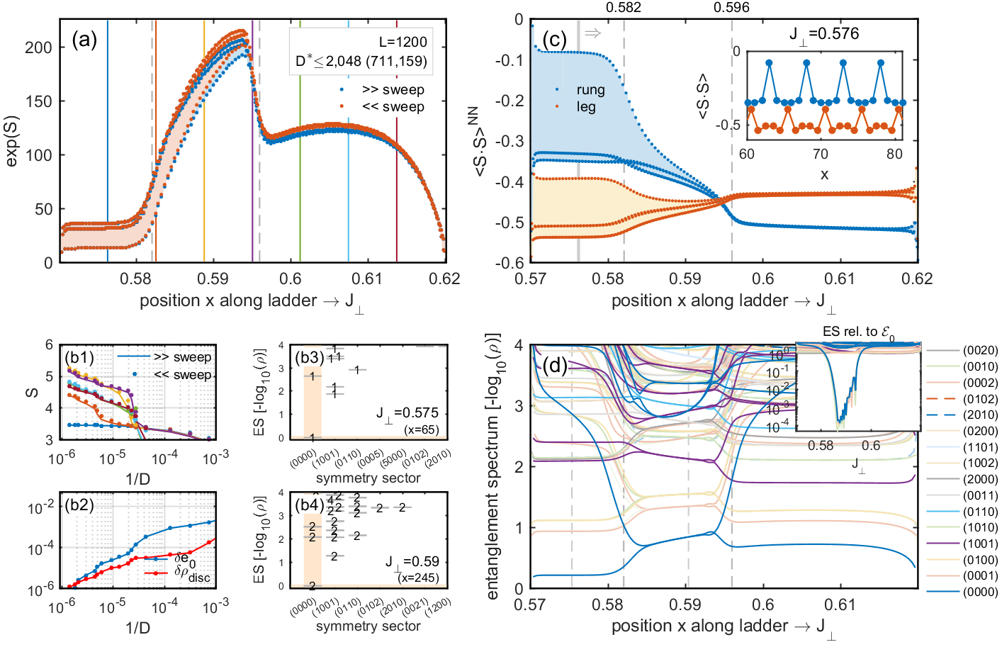
Figure D.5: DMRG scan across the narrow intermediate phase of the $\mathrm{SU}(5)$ ladder [$J_{\perp}\in[0.57,0.62]$ tuned linearly along a length $L=1200$ ladder with open boundaries, keeping up to $D^{\ast}\leq 2048$ multiplets ($D\leq 711,159$ states)] — Panel (a) shows the block entanglement entropy $S$ along the system. The intermediate phase $J_{\perp}\in[J_{\perp}^{c1},J_{\perp}^{c2}]=[0.581,0.596]$ is marked by vertical dashed lines [similar in panel (c-d)]. The data points are also connected by a line of light matching color, with the effect of shading data with significant period-5 variations for $J_{\perp}\lesssim J_{\perp}^{c2}$. Panel (b1) shows the growth of the entanglement entropy $S$ vs. $1/D$ at specific cuts $x$ along the ladder. The cuts corresponds to specific values values of $J_{\perp}$ [color matched with the vertical markers in panel (a)]. The range $J_{\perp}<J_{\perp}^{c1}$ is well converged (blue), whereas the range $J_{\perp}>J_{\perp}^{c1}$ still shows (minor) growth of the entanglement entropy for the largest $D$ employed [see remainder of data in (b), and also the increase in (a) from the last forward ($\gg$; blue dots) to the last backward sweep ($\ll$; red dots)]. Panel (b2) shows the largest discarded DMRG weight $\delta\rho_{\mathrm{disc}}$ over the entire ladder vs. $1/D$, together with the convergence $\delta e_{0}$ of the overall “ground state” energy $e_{0}\equiv E_{0}/L$. Panel (b3-4) show the entanglement spectrum in the gapped and the intermediate phase at $J_{\perp}=0.575$ and $J_{\perp}=0.590$, respectively. The number on top of each level indicates the multiplet degeneracy. Panel (c) shows the $\langle S\cdot S\rangle$ nearest-neighbor correlations where the shading again indicates period-5 variations of the corresponding data in matching color. A zoom into these variations around $J_{\perp}\simeq 0.576$ [vertical solid gray marker] is shown in the inset. Panel (d) shows the flow of entanglement spectra along the ladder, i.e. vs. $J_{\perp}$ where different color represent different symmetry sectors (see legend). The lines connect data from every 5th bond, where bonds corresponding to a block size of a multiple of 5 are shown in strong colors. The inset shows a semilog plot of the same data, yet relative to the lowest level for each bond.

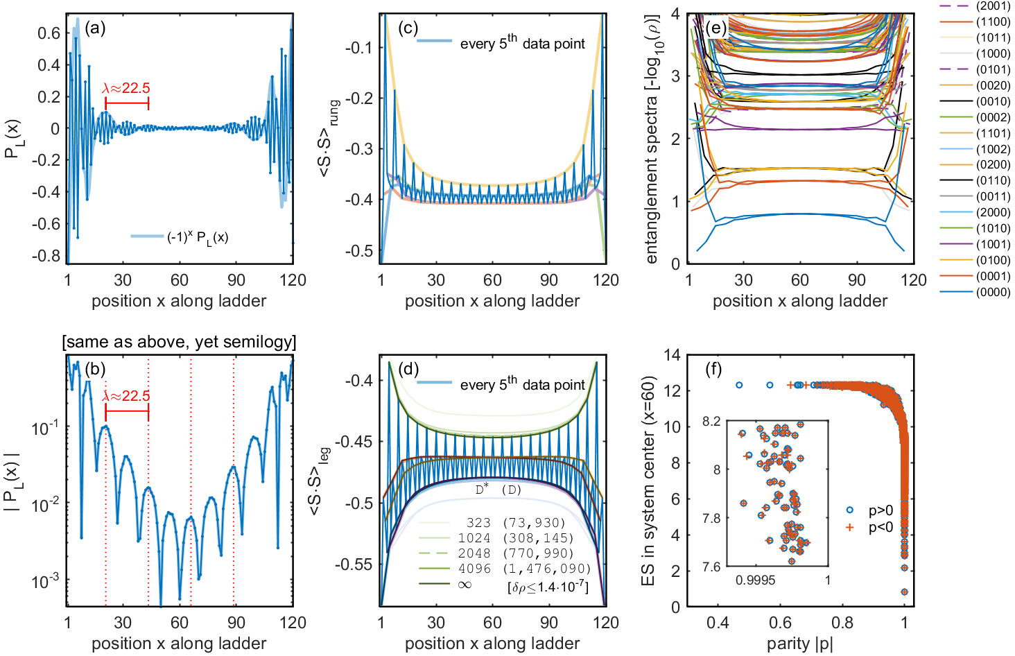
Figure D.6: Uniform $\mathrm{SU}(5)$ ladder in the middle of the intermediate phase at $J_{\perp}=0.590$. The $\mathrm{SU}(N=5)$ DMRG simulation was performed on a ladder of length $L=120$ with open boundary condition keeping up to $D{{}^{\ast}}=4096$ multiplets (about $D\leq 1.5$ million states). Panel (a) and (b) analyze the block parity $P_{L}(x)$. Up to an alternating behavior, and within finite-size variations [cf. Fig. C.4(d)], a period of $\lambda\sim 2N=10$ rungs is observed. This period is also marked via vertical dotted lines in (b). Panels (c) and (d) show the nearest-neighbor $\langle S\cdot S\rangle$ correlation along rungs and legs, respectively. Panel (d) shows convergence within DMRG by adding data lines for intermediate sweeps at $D^{\ast}$ as specified with the legend to the right, together with an extrapolation to $D^{\ast}\to\infty$. This demonstrates that the last sweep at $D^{\ast}=4096$ is already well converged. Panel (e) shows the entanglement spectra along the ladder where each line connects data from every bond, while combining data for all ladder positions $x$ [therefore e.g. only iterations where $x$ includes an integer multiple of 5 rungs support the scalar $(0000)$ symmetry sector]. Colors themselves indicate individual symmetry sectors as indicated with the legend. Again as with Fig. D.5(d), the number $n_{Y}$ of boxes in the corresponding Young tableau also identifies the rung position $x$ modulo $N$ along the ladder, i.e. $\mathrm{mod}(n_{Y},N)=\mathrm{mod}(2x,N)$, resulting in 5 data sets w.r.t. rung position. Panel (f) shows block parity vs. energy in the entanglement spectrum (see text) at fixed bond position $x=60$ in the system center based on $-\log_{10}(\rho)$. The inset shows a zoom around $ES\sim 8$ which demonstrates that a systematic pairing of multiplets with opposite rung parity occurs all the way down to eigenvalues of the block density matrix well below $10^{-8}$.

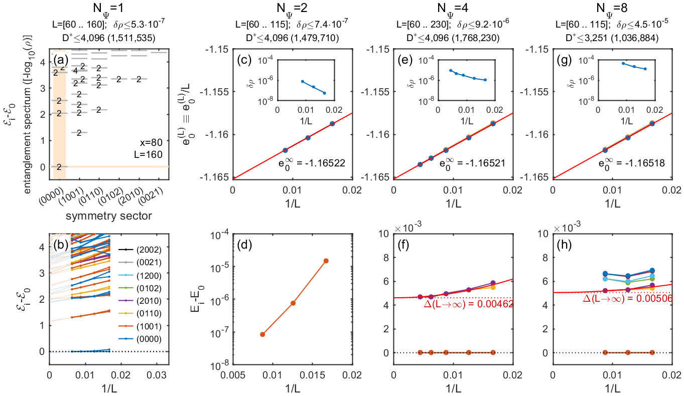
Figure D.7: Analysis of singlet gap for uniform $\mathrm{SU}(5)$ ladders up to $230$ rungs at $J_{\perp}=0.590$, i.e. in the middle of the intermediate phase. From left to right, respectively, the simulations targeted a total of $N_{\psi}=1,2,4,8$ low-energy states in the singlet sector $(0000)$. The panels in the left column, (a-b), show entanglement spectra in the center of the ladder for the ground state only. In contrast to Fig. D.5(b4), panel (a) is derived from a uniform system here. The data as in panel (a) was computed for system sizes up to $L=160$ and plotted vs. $1/L$ in panel (b). The remainder of the panels show DMRG results that simultaneously targeted multiple states. The upper panels (c-g) show ground state convergence, with the maximum discarded weight vs. $1/L$ shown as inset to each panel. The lower panels (d-h) show the energy of the excited states relative to the ground state vs. $1/L$, together with a quadratic extrapolation towards the thermodynamic limit, $L\to\infty$.

The $\mathrm{SU}(5)$ intermediate phase can already be observed in a DMRG scan across the intermediate phase, as shown in Fig. D.5. It is surrounded by a gapped phase for $J_{\perp}<J_{\perp}^{c1}$, and a critical phase for $J_{\perp}>J_{\perp}^{c2}$. Its extremely narrow range $J_{\perp}\in[J_{\perp}^{c1},J_{\perp}^{c2}]=[0.581,0.596]$ is marked by the vertical dashed lines in Fig. D.5(a,b). In contrast to the $\mathrm{SU}(3)$ ladder, the entire $\mathrm{SU}(5)$ intermediate phase ranges over a less than 2.6% variation in $J_{\perp}$. The behavior of the phase boundaries $J_{\perp}^{c1}\simeq 0.581$ and $J_{\perp}^{c2}\simeq 0.596$ has been checked vs. system size $L$ [cf. inset to Fig. 6(a)]. Somewhat reminiscent of the $\mathrm{SU}(3)$ ladder, the position $J_{\perp}^{c2}$ of the upper boundary turned out very stable, whereas the position $J_{\perp}^{c1}$ of the lower boundary moved to slightly smaller values still with increasing system size. In this sense, the intermediate phase is stable in the thermodynamic limit.

The entanglement entropy in Fig. D.5(a) shows a sharp increase in the intermediate phase which makes this phase numerically challenging. As shown in the finite $D$ scaling of the entanglement entropy in Fig. D.5(b1), the ladder is clearly converged in the gapped regime (blue data). In contrast, for both the intermediate as well as the critical large $J_{\perp}$ regime, the DMRG simulation is still not fully converged, despite keeping up to $D=711,159$ states ($D^{\ast}=2,048$ multiplets). Nevertheless, in the final sweep of the DMRG simulation the largest discarded weight over the entire chain is already as low as $\delta\rho_{\mathrm{disc}}\lesssim 10^{-6}$ [Fig. D.5(b2)]. Hence the physical picture may already be considered converged. From (b1) one can also see that in order to actually see the intermediate phase in the DMRG simulation, already a large number states was required to start with ($1/D\lesssim 3\cdot 10^{-5}$, i.e. $D\gtrsim 30,000$).

The entanglement spectrum (ES) in the gapped VBC phase at $J_{\perp}<J_{\perp}^{c1}$ [Fig. D.5(b3)] features a large gap between the lowest and first excited level with a sparse set of higher levels, as expected. By comparison, the entanglement spectrum of the intermediate phase at $J_{\perp}=0.590$ [Fig. D.5(b4)] shows a reduced gap in the entanglement spectrum, and a denser set of higher lying levels. Much more remarkably, though, it shows a systematic two-fold degeneracy in its multiplet structure. Note that this is degeneracy of multiplets which themselves have further large internal dimensions: $d(0000)=1$, $d(1001)=24$, $d(0110)=75$, $d(0102)=126$, $d(0021)=175$, etc.

Figure D.5(c) shows the nearest-neighbor $\langle S\cdot S\rangle$ correlations along the ladder. For large $J_{\perp}$, the translational symmetry breaking along the chain diminishes [see Fig. D.5(c), for $J_{\perp}>J_{\perp}^{c2}$, except close to the open right boundary]. This is consistent with a gapless, i.e. critical phase. In the gapped VBC phase $J_{\perp}<J_{\perp}^{c1}$ a clear 5-rung periodicity is observed (see inset). In particular, the $\langle S\cdot S\rangle$ bonds along the legs (orange) clearly break up into blocks of 5 rungs, i.e. they have 4 consecutive tight bonds followed by a weak link (see also cartoon in Fig. 1). This VBC block size is natural as it represents the smallest unit in given $\mathrm{SU}(5)$ ladder that can harbor a singlet state. In stark contrast, while also the rung data (blue) exhibits a 5-rung periodicity, it is the central rung within each VBC unit that is bound most weakly (compare blue to orange data in inset), hence gathers most of the weight from the presence of a symmetric rung multiplet. This is in agreement with the AASAA cartoon picture discussed in Sec. III.2.1 that reduces to an approximate resonating valence bond picture ASA on the circumference in the case of $\mathrm{SU}(3)$ [cf. Fig. 4(a)].

The physical state changes strongly across the intermediate phase. E.g. when zooming out of Fig. D.5(c) to show a more extended range $J_{\perp}\in[0,1]$, the transition in $\langle S\cdot S\rangle_{\perp}$ almost looks like a jump to values that differ by about a factor of 2. Eventually, however, the intermediate phase allows for a smooth transitioning. In contrast to the critical phase for large $J_{\perp}$, the symmetry breaking appears to persist along the intermediate phase, even though it is further reduced when analyzing larger uniform $\mathrm{SU}(5)$ ladders [cf. inset to Fig. 6(a)].

Figure D.5(d) shows the entanglement spectra along the ladder, i.e. an “entanglement flow diagram” vs. $J_{\perp}$. The individual lines connect data from every 5th bond, where the data from bonds the correspond a block size of a multiple of 5 are shown in strong colors. These entanglement spectra again also differ starkly for the intermediate phase as compared to the small and large $J_{\perp}$ phases. The 2-fold multiplet degeneracy already seen in Fig. D.5(b4) is persistent throughout the entire intermediate phase. The data in the main panel Fig. D.5(d) is replotted in its inset relative to the lowest level for each bond. This shows that the splitting of the lowest pair of levels drops quickly to extremely small values within the intermediate phase.

The $\mathrm{SU}(5)$ ladder is commensurate in short-ranged correlations for uniform ladder as, e.g. as shown in Fig. D.6 at $J_{\perp}=0.590$ in the middle of the intermediate phase. In particular, the nearest-neighbor $\langle S\cdot S\rangle$ correlations along both, rungs [Fig. D.6(c)] and legs [Fig. D.6(d)] show a clean 5-rung periodicity.

However, there are traces of incommensuration also in the $\mathrm{SU}(5)$ intermediate phase. For example, the minor oscillatory behavior towards the upper boundary $J_{\perp}^{c2}$ in Fig. D.5(d) [in particular, see also inset] may be interpreted as the onset of incommensurate behavior. This is even more pronounced still in the block parity $P_{L}(x)$ shown in Fig. D.6(a) that shows a tunable wavelength with $J_{\perp}$. In particular, the wavelength seen in Fig. D.6(a) becomes shorter as $J_{\perp}$ is reduced and moves closer to $J_{\perp}^{c1}$. In stark contrast to the $\mathrm{SU}(3)$ ladder [e.g. see Fig. C.4(d)], the data in Fig. D.6(a) decays approximately exponentially towards the bulk of the ladder, as seen in the semilog plot in Fig. D.6(b). However, an analysis along the lines of Fig. C.4 for the $\mathrm{SU}(3)$ ladder earlier did not support a global signature of incommensurate behavior for the $\mathrm{SU}(5)$ ladder (data not shown). Specifically, there was no indication for an alternation in the ground state parity with increasing system size.

The rapid systematic pairing of multiplets away from the open boundary was already seen in the entanglement flow in the DMRG scan in Fig. D.5(d), and is again also encountered for uniform ladders as in Fig. D.6(e). The origin of this systematic pairing in the intermediate phase is related to the rung parity, in that it is multiplets of opposite rung parity that pair up. This is demonstrated in Fig. D.6(f). The systematic pairing and correlation with the rung parity holds for states with weight down to less than $10^{-8}$ in the reduced density matrix! For Fig. D.6(f), the block density matrix $\rho(x)$ for sites $x^{\prime}>x$ for fixed bond $x=60$ in the system center was compared to the matrix elements $P(x)$ of the swap operator for all rungs $x^{\prime}<x$ in the DMRG basis at bond $x$ [therefore, e.g. $P_{L}(x)=\mathrm{Tr}(\rho(x)P(x))$]. The simultaneous (approximate) diagonalization of both, $\rho(x)$ and $P(x)$, for the data in Fig. D.6(f) was performed separately for each individual symmetry sector as follows: (i) the effective many body state space at bond $x$ was split into symmetric ($p>0$) and antisymmetric ($p<0$) states by first diagonalizing $P(x)$. (ii) Then the reduced density matrix $\rho(x)$ was mapped into these parity sectors, and diagonalized to obtain the entanglement spectra [ES, using $-\log_{10}\mathrm{eig}(\rho)$; vertical data in Fig. D.6(f)], as well as the final basis. The latter (iii) was used to compute the expectation values of the parity $p$ [horizontal data in Fig. D.6(f)] which via (i) results in values very close to $\pm 1$ paired up in energy.

In order to tackle the question whether the intermediate phase is gapped, we compute excited states within our DMRG, followed by finite size scaling. The results are shown in in Fig. D.7. There we compare data from DMRG simulations in the intermediate phase at $J_{\perp}=0.590$ that simultaneously targeted $1,2,4$, and $8$ states from left to right panels, respectively. All states belonged to the singlet sector, therefore the following discussion concerns the singlet gap of the $\mathrm{SU}(5)$ ladder. The scaling of the entanglement spectra in the center of ground states for ladders of length $L$ in Fig. D.7(b) shows a pronounced entanglement gap that persist in the thermodynamic limit when extrapolating vs. $1/L\to 0$.

When simultaneously targeting multiple state, the matrix product state (MPS) of DMRG Affleck (1988a); Rommer and Östlund (1997); Verstraete and Cirac (2004); Schollwöck (2005, 2011) acquires an additional index that references the individual states. Depending whether this index is associated with the left or the right of a given bond in the ladder, the entanglement spectra looks different. Hence when targeting $N_{\Psi}>1$ states, entanglement spectra become less useful. Therefore the remainder of the panels, Fig. D.7(c-h), focus on the analysis of global energy convergence. The upper panels, Fig. D.7(c,e,g), show a consistent convergence of the ground state energy per site, suggesting $e_{0}^{\infty}=-1.16522$ [most accurate value for $N_{\Psi}=2$, panel (c); larger $N_{\Psi}$ for the same or smaller bond dimension $D$ naturally leads to slightly less accurate values, as also seen in the overall trend with increasing $N_{\Psi}$ in the discarded weights in the insets].

The lower panels, Fig. D.7(d,f,h) analyze the energy of the excited energy eigenstates relative to the ground state energy. The systematic 2-fold degeneracy of the entanglement spectra for the ground state [cf. Fig. D.7(a)] is inherited when computing excited energy eigenstates of the full system. This is plausible given the interpretation obtained from Fig. D.6(e-f) that the systematic degeneracy of the entanglement spectra is related to states of opposite rung-parity. Hence the energy splitting between ground state and first excited state diminishes in the thermodynamic limit, as seen in Fig. D.7(d).

When including the next two degenerate states, the finite size scaling in Fig. D.7(f) reveals that this state remain separated by a small but finite energy gap of about $\Delta\simeq 0.004$ in the thermodynamic limit. When including another four states in the last column of Fig. D.7(g-h), these additional states are already close to the excited states encountered in Fig. D.7(f). Therefore even though the estimated gap $\Delta$ is on the order of $1/L$ for the largest system size in Fig. D.7(f), we interpret the weak dependence of the energy splitting on $1/L$, indeed, as indication for a small but finite energy gap.

Appendix E DMRG study of the $N=3$ and $N=5$ large $J_{\perp}$ regime

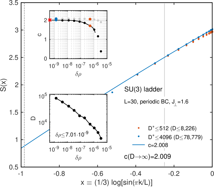
Figure E.8: Central charge for $\mathrm{SU}(3)$ ladder in the large $J_{\perp}$ phase, actually having $J_{\perp}=1.6$ just above $J_{\perp}^{c2}=1.562$, based on the scaling of the block entanglement entropy using periodic boundary conditions (see Calabrese and Cardy (2009); Amico et al. (2008) and also text). For fixed number of $D\to\infty$ kept states ($D^{\ast}$ multiplets), quadratic fit for the range $x>x_{0}=-0.25$ (see vertical gray marker) e.g. results in the blue line for the last DMRG sweep performed. Its slope at $x=0$ yields the central charge $c=2.008$ as indicated with the legend. The left dotted marker indicates $(1/3)\log(L/\pi)$. Therefore with $4$ data points between this marker and the one at $x_{0}$, the overwhelming part of the ladder ($22$ rungs out of $30$ rungs) fall into $x>x_{0}$). The upper inset analyses the convergence of the central charge vs. average discarded weight $\delta\rho$ for given DMRG sweep at fixed $D$. The data was obtained by evaluating the slope of $S(x)$ as shown in the main panel for fixed $D$ at $x=x_{0}$ and $x=0$ (gray and black data, respectively). The red asterisk corresponds to the extrapolated value $D\to\infty$ as specified with the legend in the main panel. The lower inset shows discarded weight $\delta\rho$ vs. number $D$ of kept states.

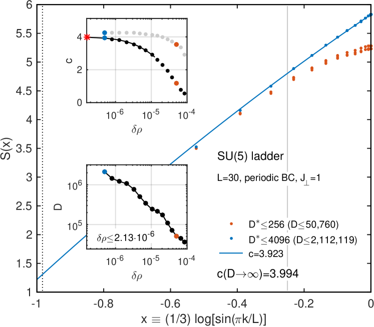
Figure E.9: Central charge for $\mathrm{SU}(5)$ ladder in the large $J_{\perp}$ phase for $L=30$, with an analysis of the entanglement entropy that is completely analogous to the case of $\mathrm{SU}(3)$ in Fig. E.8. In the extrapolated limit $D\to\infty$ and by evaluating the slope at $x=0$, this yields a central charge of $c=3.994$ (see legend and also red asterisk in upper inset), in excellent agreement with the expected value of $c=4$.

For large rung coupling $J_{\perp}$, as explained in the main text, an $\mathrm{SU}(N)$ ladder maps onto an effective chain where each site transforms according to the antisymmetric irrep ( ${\tiny\yng(1,1)}$ ) of $\mathrm{SU}(N)$. For odd $N$ (such as $N=3$ and $N=5$), such a system is predicted to be critical and can be described by conformal field theories. Numerically, the corresponding central charges can be determined from the scaling of the block entanglement entropy of a contiguous block of length $k$ rungs for a ladder of length $L$ with periodic boundaries, Calabrese and Cardy (2009); Amico et al. (2008),

$$S(k) = \tfrac{c}{3}\log\bigl{[}\tfrac{L}{\pi}\sin(\tfrac{\pi k}{L})\bigr{]}+\mathrm{const}$$ (23)

$$\equiv c\cdot\underbrace{\tfrac{1}{3}\log\bigl{[}\sin(\tfrac{\pi k}{L})\bigr{]}}_{\equiv x}+\mathrm{const}^{\prime}\text{.}$$ (24)

This allows to extract the central charge $c$ from the slope of $S(x)$ around $x\simeq 0$, which is equivalent to evaluating the curvature of $S(k$) in the center of the system. Having periodic boundary conditions, finite size effects are strongly reduced as compared to open boundary conditions, hence fairly short systems often suffice (here $L=30$). This is important, since the entanglement entropy is about twice as large as compared to a system with open boundary conditions. In the DMRG simulations, in practice, the periodic boundary was dealt with by folding a circle of $L$ rungs into a double ladder of length $L/2$ each, that are connected at the ends and otherwise have interleaved rungs from the upper and lower half-ladder, respectively. This construction avoids a long range coupling term in the Hamiltonian across the entire system. The resulting system then, while expensive in any case, has effectively an open left and right boundary with at most 4th-nearest-neighbor interactions which is beneficial for DMRG.

The central charge is evaluated for subsequent DMRG sweeps at fixed $D$ each, where $D$ is ramped exponentially $D\to\sqrt{2}D$ from one sweep to the next. Each sweep also results in some average discarded weight $\delta\rho$. Since the behavior of $\delta\rho$ vs. $D$ is somewhat irregular [see lower inset in Fig. E.8 and, in particular, also later for the case of $\mathrm{SU}(5)$ in Fig. E.9], the analysis of the central charge is performed vs. $\delta\rho\to 0$ and not vs. $1/D\to 0$. This results in much smoother data that is better suited for quadratic polynomial extrapolation.

The resulting data for the central charge for the $\mathrm{SU}(3)$ ladder at strong coupling is shown in Fig. E.8. Even though $J_{\perp}$ is just across the boundary of the intermediate phase ($J_{\perp}=1.60>J_{\perp}^{c2}=1.562$), a length $L=30$ already yields a central charge $c=2$ to better than 1%, which is in agreement with the expected central charge from conformal field theory (CFT), $c=N-1$ [see Fig. 1 in the main text]. From the analysis in the upper inset (gray vs. black data) one can conclude, that in given case a periodic ladder of up to $L=9$ rungs, i.e. significantly shorter than the chosen $L=30$, already also would yield a central charge reasonably close to $c\simeq 2$. But uncertainty margins are significantly reduced by going to somewhat larger system sizes.

Similarly, the $\mathrm{SU}(5)$ ladder at large rung coupling $J_{\perp}$ becomes critical with a central charge $c=N-1=4$. By analysis of the entanglement entropies, this is confirmed in Fig. E.9 at $J_{\perp}=1$, again to within an uncertainty of less than 1%. This calculation explicitly goes beyond a million of kept states in the DMRG. Once all symmetry related generalized Clebsch-Gordan coefficients are computed once and for all Weichselbaum (2012), this calculation runs an a regular state-of-the-art workstation within several days.