Exchange-correlation functionals of i-DFT for asymmetrically coupled leads

Abstract

A recently proposed density functional approach for steady-state transport through nanoscale systems (called i-DFT) is used to investigate junctions which are asymmetrically coupled to the leads and biased with asymmetric voltage drops. In the latter case, the system can simply be transformed to a physically equivalent one with symmetric voltage drop by a total energy shift of the entire system. For the former case, known exchange correlation gate and bias functionals have to be generalized to take into account the asymmetric coupling to the leads. We show how differential conductance spectra of the constant interaction model evolve with increasing asymmetry of both voltage drops and coupling to the leads.

1 Introduction

The measurement of electronic transport through nanoscale devices provides an important means for probing the electronic and magnetic structure and related properties of the system. For example, the measurement of the zero-bias conductance of atomic-scale metallic nanocontacts formed in break-junction experiments unveiled conductance quantization and the formation of monoatomic chains in these systems Agrait:PR:2003 . Conductance spectroscopy of quantum dots coupled to conducting electrodes demonstrated Kondo effect and Coulomb blockade phenomena Goldhaber-Gordon:Nature:1998 ; Park:Nature:2002 ; Grabert:book:1992 ; Champagne:NL:2005 . Using scanning tunneling microscope spectroscopy (STS), the Kondo effect and spin excitations of magnetic adatoms and molecules on conducting substrates can be measured Madhavan:Science:1998 ; Li:PRL:1998 ; Knorr:PRL:2002 ; Zhao:Science:2005 ; Iancu:NL:2006 ; Hirjibehedin:Science:2007 ; Parks:Science:2010 ; Oberg:NNano:2014 ; Karan:NL:2018 . Coupling of the electronic degrees of freedom to the nuclear motion even allows to determine phonon band structures of metals or vibronic excitations of molecules by inelastic electron transport spectroscopy (IETS) Stipe:Science:1998 ; Hahn:PRL:2000 .

The theoretical description of electronic transport in nanoscale systems either involves sophisticated and often computationally demanding many-body treatments of relatively simple model Hamiltonians, or ab initio approaches based on density functional theory (DFT) Lang:95 which allows to treat realistic systems of substantial sizes (up to thousands of atoms depending on the implementation). The description of (steady-state) transport through a nanoscale system within the framework of DFT goes back to a seminal paper by Lang Lang:95 . In this work, following ideas of Landauer Landauer:57 and Büttiker Buettiker:86 , steady-state transport is treated as a scattering problem of effectively non-interacting electrons where the local Kohn-Sham (KS) potential in the nanoscale region C is treated as the scattering potential. The resulting scheme, often called LB+DFT, today is basically the method of choice for the ab initio description of electronic transport. Conceptually, however, there is a problem: since DFT is a ground state or equilibrium theory, there is no guarantee that the LB+DFT formalism yields the correct non-equilibrium density and current, even if the exact KS potential is used. Importantly, for this reason many-body phenomena such as the Kondo effect or Coulomb blockade are not described properly in the finite bias transport characteristics of the system within the LB+DFT approach StefanucciKurth:15 .

A combination of the DFT based transport approach with more sophisticated many-body treatments of model Hamiltonians, allows to incorporate strong electronic correlations originating from a relatively small subspace (e.g. the $d$-shell of a transition metal atom), into the description of electronic transport through realistic systems Jacob:JPCM:2015 ; Droghetti:PRB:2017 . The drawback of this approach is that, like all DFT++ approaches, it is hampered by the infamous double-counting problem and the determination of the effective interaction strength of the strongly correlated subspace(s), thus limiting the predictivity of the approach.

It is thus desirable to have an approach that treats the whole nanoscale system on the same footing, while at the same time being computationally affordable, in order to be able to treat realistic systems. In principle, time-dependent DFT (TDDFT) RungeGross:84 provides a proper DFT framework to treat non-equilibrium situations such as transport. Indeed it has been shown that in the steady state which develops in the long-time limit after switch-on of a DC bias, TDDFT in principle leads to corrections to the LB+DFT formalism sa-2.2004 ; ewk.2004 ; kbe.2006 ; skgr.2007 .

In the present work we will use yet another DFT framework for steady-state transport, called i-DFT, which has been proposed only recently StefanucciKurth:15 . This approach is comparable to the LB+DFT formalism in computational effort. However, since i-DFT is an in principle exact approach for the out-of-equilibrium steady state, it is capable of describing many-body effects in transport provided good approximations to the i-DFT functionals are available. In fact, already in Ref. StefanucciKurth:15 a functional for the so-called constant interaction model (CIM) has been developed which correctly describes the Coulomb blockade at arbitrary bias. This approximation has later been augmented to also include Kondo physics, first for the the single-impurity Anderson model (SIAM) Kurth:PRB:2016 and later for the CIM with an arbitrary number of levels Kurth:JPCM:2017 . All the functionals mentioned so far were constructed for the case of symmetric coupling to the leads. Very recently, an approximation for the CIM at extremely asymmetric coupling has also been developed Jacob:NL:2018 .

For the decription of realistic transport setups such as a quantum dot coupled to leads or a molecule probed by an STM, it is necessary to consider arbitrary asymmetric coupling to the leads in the i-DFT approach. Here we construct i-DFT functionals for the CIM at arbitrary asymmetry in the coupling to the leads and compare their relative performance.

2 Density functional theory for steady state transport: i-DFT

2.1 Transport setup

We are interested in the generic situation sketched schematically in Fig. 1 where a central nanoscopic region C is coupled to macroscopic left (L) and right (R) leads. The system is driven out of equilibrium by applying a (DC) bias across region C and we are interested in the resulting steady-state current. We emphasize that here we just assume that the system reaches a steady state after application of the bias but we do not address the question how this steady state is reached (i.e., we are not interested in the time evolution towards the steady state). The Hamiltonian describing the system coupled to leads is given by

$$\hat{\mathcal{H}}=\hat{\mathcal{H}}_{\rm C}+\hat{\mathcal{H}}_{\rm L}+\hat{\mathcal{H}}_{\rm R}+\hat{\mathcal{V}}_{{\rm L}}+\hat{\mathcal{V}}_{{\rm R}}$$ (1)

where $\hat{\mathcal{H}}_{\rm C}$ describes the nanoscopic region, $\hat{\mathcal{H}}_{\alpha}$ describes lead $\alpha$ ($\alpha\in\{L,R\}$) and $\hat{\mathcal{V}}_{\alpha}$ is the coupling between lead $\alpha$ and region C. For simplicity, the two leads are considered as non-interacting, i.e., $\hat{\mathcal{H}}_{\alpha}=\sum_{q\sigma}\epsilon^{\alpha}_{q}\hat{c}_{\alpha,q\sigma}^{\dagger}\hat{c}_{\alpha,q\sigma}$. In contrast, in the central region we allow for a general electron-electron interaction such that the Hamiltonian $\hat{\mathcal{H}}_{\rm C}$ takes the form

$$\hat{\mathcal{H}}_{\rm C}=\sum_{i,j,\sigma}h_{ij}^{0}\,\hat{d}^{\dagger}_{i\sigma}\hat{d}_{j\sigma}+\frac{1}{2}\sum_{{i,j,k,l}\atop{\sigma,\sigma^{\prime}}}U_{ijkl}\,\hat{d}^{\dagger}_{i\sigma}\hat{d}^{\dagger}_{j\sigma^{\prime}}\hat{d}_{l\sigma^{\prime}}\hat{d}_{k\sigma}$$ (2)

where $\bm{h}^{0}=\bm{t}+\bm{v}$ is the one-body part of the Hamiltonian (in matrix notation) comprising the kinetic energy $\bm{t}$ and external potential (gate) $\bm{v}$, and $U_{ijkl}$ are the matrix elements of the electron-electron interaction. The coupling between the central region and the two leads L and R is described by

$$\hat{\mathcal{V}}_{\alpha}=\sum_{i,q,\sigma}V^{\alpha}_{q,i}\,\hat{c}^{\dagger}_{\alpha,q\sigma}\hat{d}_{i\sigma}+{\rm h.c.}$$ (3)

Integrating out the degrees of freedom of lead $\alpha$ yields the corresponding embedding self-energy

$$\bm{\Sigma}_{\alpha}(\omega)=\bm{V}_{\alpha}^{\dagger}\frac{1}{\omega-\bm{H}_{\alpha}}\bm{V}_{\alpha}$$ (4)

where $\bm{V}^{\alpha}=\left(V^{\alpha}_{q,i}\right)$ and $\bm{H}_{\alpha}=\left(\epsilon_{q}^{\alpha}\right)$. The anti-hermitian part of the embedding self-energy yields the so-called coupling matrix, $\bm{\Gamma}_{\alpha}=i(\bm{\Sigma}_{\alpha}^{\dagger}-\bm{\Sigma}_{\alpha})$, which describes the broadening of the central region due to the coupling to lead $\alpha$.

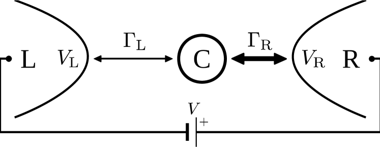
Figure 1: Schematic sketch of a nanoscale junction under an applied bias $V$. The central region (C) is coupled to two semi-infinite leads L and R. The coupling to the left and right leads may differ, i.e. ${\bm{\Gamma}}_{\rm L}\neq{\bm{\Gamma}}_{\rm R}$ in general. The voltage drop $V$ across the nanoscale junction is defined by the electrochemical potentials $V_{\rm L}$ and $V_{\rm R}$ in the two leads, $V=V_{\rm L}-V_{\rm R}$.

Finally, a bias voltage $V$ is applied between the two leads, defined by the difference in their electrochemical potentials, $V=V_{\rm L}-V_{\rm R}$, which drives the system out of equilibrium and induces a steady current $I$ across the nanoscale junction.

2.2 Steady state transport with density functional theory and foundation of the i-DFT formalism

Here we make use of the i-DFT formalism in order to describe the steady state density and current of an interacting system under a DC bias StefanucciKurth:15 . In i-DFT, one first establishes (under certain conditions KurthStefanucci:17 ) the existence of a one-to-one map between the gate potential $v(\bm{r})$ in region C and the bias $V$ symmetrically applied across it on the one hand and the steady state density $n(\bm{r})$ and current $I$ on the other hand. In a second step, just as in standard DFT, one maps the interacting problem onto a ficticious non-interacting one which exactly yields the density and current of the interacting system. This fictitious non-interacting KS system now features two potentials, the KS gate potential $v_{s}(\bm{r})$ (in region C) and the KS bias $V_{s}$. Overall this establishes a one-to-one map between the potentials of the original interacting system $(v(\bm{r}),V)$ and the ones of the KS system $(v_{s}(\bm{r}),V_{s})$, i.e.,

$$(v(\bm{r}),V)\longleftrightarrow(n(\bm{r}),I)\longleftrightarrow(v_{s}(\bm{r}),V_{s})$$ (5)

and therefore both $(v(\bm{r}),V)$ and $(v_{s}(\bm{r}),V_{s})$ are functionals of $n(\bm{r})$ and $I$. The difference between these functionals allows to define the Hartree exchange correlation (Hxc) gate potential, $v_{\rm Hxc}[n,I](\bm{r})=v_{s}[n,I](\bm{r})-v[n,I](\bm{r})$, as well as the exchange correlation (xc) bias, $V_{\rm xc}[n,I]=V_{s}[n,I]-V[n,I]$. In general, of course, the exact form of these functionals is unknown and one has to resort to approximations in practice.

In the i-DFT framework the steady-state density and current of an interacting system for given fixed external potential $v(\bm{r})$ and bias $V$ applied symmetrically in left and right leads can be calculated by solving the following coupled self-consistent KS equations StefanucciKurth:15 ; Kurth:JPCM:2017

$$n_{\rm sym}[v,V](\bm{r} = 2\sum_{\alpha={\rm L},{\rm R}}\int\frac{d\omega}{2\pi}f\left(\omega+s_{\alpha}\frac{V_{s}}{2}\right)A_{\alpha;v_{s}}(\bm{r};\omega)$$

$$I_{\rm sym}[v,V]=2\sum_{\alpha={\rm L},{\rm R}}s_{\alpha}\int\frac{d\omega}{2\pi}f\left(\omega+s_{\alpha}\frac{V_{s}}{2}\right)T_{v_{s}}(\omega)$$ (6b)

where $A_{\alpha}(\bm{r};v_{s};\omega)=\left\langle\bm{r}\right|\bm{A}_{\alpha;v_{s}}(\omega)\left|\bm{r}\right\rangle$ is the spatial representation of $\bm{A}_{\alpha;v_{s}}=\bm{G}_{v_{s}}\bm{\Gamma}_{\alpha}\bm{G}_{v_{s}}^{\dagger}$, the partial KS spectral function of C associated with electron injection from electrode $\alpha$. $T_{v_{s}}(\omega)={\rm Tr}[{\bm{\Gamma}}_{\rm L}\bm{G}_{v_{s}}^{\dagger}{\bm{\Gamma}}_{\rm R}\bm{G}_{v_{s}}]$ is the KS transmission function and $\bm{G}_{v_{s}}=(\omega-\bm{h}_{s}-\bm{\Sigma}_{\rm L}-\bm{\Sigma}_{\rm R})^{-1}$ is the (retarded) non-equilibrium KS Green function of the sample region, and $\bm{h}_{s}=\bm{t}+\bm{v}_{s}$ the KS Hamiltonian in matrix notation. Finally, $f(x)=[1+\exp(\beta x)]^{-1}$ is the Fermi function at inverse temperature $\beta$, and $s_{\alpha}=-1$ for $\alpha={\rm L}$ and $s_{\alpha}=+1$ for $\alpha={\rm R}$.

Fig. 2 shows a schematic energy diagram of the KS potentials of the system both in equilibrium (left panel) when $V_{\alpha}^{s}=V_{s}=V=0$, and out of equilibrium (right panel) for a bias voltage $V>0$ applied symmetrically between both electrodes, $V_{\rm L}^{s}=V_{s}/2=-V_{\rm R}^{s}>0$. Note that the KS bias $V_{s}$ does not only shift the chemical potentials of the leads by $\pm{V}_{s}/2$ but also the band structure of the leads. Hence for a KS bias $V_{s}$ the embedding self-energies of the electrodes (4) and accordingly the coupling matrices are to be evaluated at $\omega=\pm{V_{s}}/2$, i.e. $\bm{\Sigma}_{\alpha}=\bm{\Sigma}_{\alpha}(\omega+s_{\alpha}{V_{s}}/2)$ and $\bm{\Gamma}_{\alpha}=\bm{\Gamma}_{\alpha}(\omega+s_{\alpha}{V_{s}}/2)$.

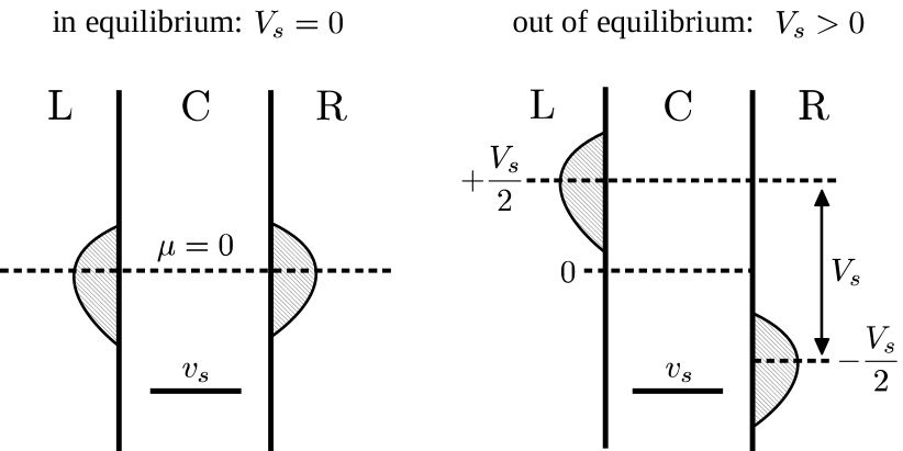
Figure 2: Schematic energy diagram of effective KS potentials $v_{s}$ and $V_{s}$ and electrode band structures (grey areas) for the nanoscale junction in equilibrium (left) and out of equilibrium (right) with symmetric voltage drop, $\pm{V_{s}/2}$.

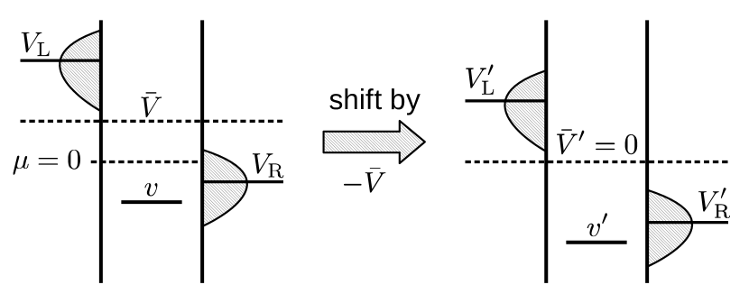
Figure 3: Transformation from a general asymmetric voltage drop $V_{\rm L}\neq-V_{\rm R}$ (left) to a symmetric voltage drop $V_{\rm L}=V/2$ and $V_{\rm R}=-V/2$ (right) by a total energy shift of $-\bar{V}=-(V_{\rm L}+V_{\rm R})/2$.

Let us now consider the situation of an arbitrary voltage drop across the junction, as depicted schematically in the left panel of Fig. 3, when the electrochemical potentials of the two leads are not symmetrically displaced from equilibrium, i.e. $V_{\rm L}\neq-V_{\rm R}$. A transformation from an arbitrary voltage drop to a symmetric voltage drop $V_{\rm L}^{\prime}=-V_{\rm R}^{\prime}=V/2$ that leaves the physical observables unchanged can be achieved by applying a spatially constant energy shift of the entire system by $-\bar{V}=-(V_{\rm L}+V_{\rm R})/2$ relative to the equilibrium chemical potential, as depicted in Fig. 3. Hence the KS equations for the particle density $n(\bm{r})$ and current $I$ for an arbitrarily distributed voltage drop $V=V_{\rm L}-V_{\rm R}$ can be obtained from the KS equations for symmetric bias (LABEL:eq:dens,6b) by shifting the KS gate $v_{s}$ by $-\bar{V}$:

$$n_{\rm asym}[v,V_{\rm L},V_{\rm R}](\bm{r})=n_{\rm sym}[v-\bar{V},V](\bm{r})$$ (7a)

$$\hskip 4.30554pt=2\sum_{\alpha={\rm L},{\rm R}}\int\frac{d\omega}{2\pi}f\left(\omega+s_{\alpha}\frac{V_{s}}{2}\right)A_{\alpha;v_{s}-\bar{V}}(\bm{r};\omega)$$

$$I_{\rm asym}[v,V_{\rm L},V_{\rm R}]=I_{\rm sym}[v-\bar{V},V]$$ (7b)

$$\hskip 4.30554pt=2\sum_{\alpha={\rm L},{\rm R}}s_{\alpha}\int\frac{d\omega}{2\pi}f\left(\omega+s_{\alpha}\frac{V_{s}}{2}\right)T_{v_{s}-\bar{V}}(\omega)$$

Note that the embedding self-energies and coupling matrices are still to be evaluated at $\pm{V_{s}}/2$; only the KS gate $v_{s}$ is shifted by $-\bar{V}$. Hence the KS GF in the transformed system is given by:

$$\bm{G}_{v_{s}-\bar{V}}(\omega)=\frac{1}{\omega-\bm{h}_{s}+\bar{V}-\sum_{\alpha={\rm L},{\rm R}}\bm{\Sigma}_{\alpha}\left(\omega+s_{\alpha}\frac{V_{s}}{2}\right)}$$ (8)

One can also introduce a KS voltage drop $V_{\alpha}^{s}$ distributed with the same ratio as the actual voltage $V$ between both leads, $V_{\alpha}^{s}=V_{s}(V_{\alpha}/V)$ by performing a simple change of the integration variable according to $\omega\rightarrow\omega-\bar{V}_{s}$ where $\bar{V}_{s}\equiv(V_{\rm L}^{s}+V_{\rm R}^{s})/2$. Similarly, the arguments to the electrode quantities (embedding self-energies, coupling matrices and Fermi functions), change according to $\omega-s_{\alpha}{V_{s}/2}\rightarrow\omega-V^{s}_{\alpha}$. We thus obtain the i-DFT KS equations for asymmetric voltage drops:

$$n_{\rm asym}[v,V_{\rm L},V_{\rm R}](\bm{r}) = 2\sum_{\alpha}\int\frac{d\omega}{2\pi}f\left(\omega-V_{\alpha}^{s}\right)\bar{A}^{\alpha}_{v_{s}-\bar{V}_{\rm xc}}(\bm{r};\omega)$$

$$I_{\rm asym}[v,V_{\rm L},V_{\rm R}] = 2\sum_{\alpha}s_{\alpha}\int\frac{d\omega}{2\pi}f\left(\omega-V_{\alpha}^{s}\right)\bar{T}_{v_{s}-\bar{V}_{\rm xc}}(\omega)$$

(9b)

where $\bar{V}_{\rm xc}=\bar{V}_{s}-\bar{V}$ is the average xc bias of both leads and the spectral function $\bar{A}^{\alpha}_{v_{s}}$ and transmission function $\bar{T}_{v_{s}}$ refer to a new KS GF for arbitrary chemical potentials $V^{s}_{\alpha}$ of the leads

$$\bm{\bar{G}}_{v_{s}}(\omega)=\frac{1}{\omega-\bm{h}_{s}-\sum_{\alpha={\rm L},{\rm R}}\bm{\Sigma}_{\alpha}\left(\omega-V_{\alpha}^{s}\right)}.$$ (10)

2.3 i-DFT functionals for the Constant Interaction Model at asymmetric coupling

We now apply the i-DFT formalism described above to the so-called constant interaction model (CIM) which is widely used as a model for the description of effects of strong electronic correlation such as Coulomb blockade (CB) or the Kondo effect. The CIM Hamiltonian can be obtained from Eq. (2) by simplifying the Coulomb interaction in the central region according to $U_{ijkl}=U\delta_{ik}\delta_{jl}$. Additionally we assume a diagonal one-body part $h^{0}_{ij}=\varepsilon_{i}\delta_{ij}$ which leads to

$$\mathcal{H}_{\rm C}^{\rm CIM}=\sum_{i\sigma}\varepsilon_{i}\,\hat{n}_{i\sigma}+\frac{U}{2}\sum_{i\sigma\neq{j\sigma^{\prime}}}\hat{n}_{i\sigma}\hat{n}_{j\sigma^{\prime}}$$ (11)

where $\hat{n}_{i\sigma}$ is the electron occupation operator for level $i$ with spin $\sigma$. We furthemore assume that the coupling matrices $\bm{\Gamma}_{\alpha}$ are energy independent, i.e., we are in the wide-band limit (WBL) for both leads. Note that for a single level this becomes the single-impurity Anderson model (SIAM)Anderson:PR:1961 .

The CIM has been studied within the i-DFT framework both in the Coulomb blockade StefanucciKurth:15 as well as in the Kondo regime Kurth:PRB:2016 ; Kurth:JPCM:2017 and approximate i-DFT xc potentials have been suggested. However, these approximations were restricted to symmetric coupling. In a very recent work Jacob:NL:2018 we have designed an approximation for the limiting case of an extremely asymmetrically coupled CIM where the coupling to one of the leads becomes infinitesimal. We were interested in this extreme limit because it can be shown that in this limit one can extract equilibrium many-body spectral functions at zero temperature from differential conductances computed with i-DFT Jacob:NL:2018 . In the present work we are interested in arbitrary asymmetry in the coupling and we thus need to construct xc potentials for this case as well. For simplicity, we restrict ourselves to the CIM with an arbitrary number of degenerate single-particle levels ($\varepsilon_{i}=\varepsilon$) which are all coupled in the same way to the lead $\alpha$, i.e., the coupling matrices in the single-particle basis $\bm{\Gamma}_{\alpha}=\gamma_{\alpha}{\mathbf{1}}$ are proportional to the unit matrix $\mathbf{1}$ (but the constants $\gamma_{\rm L}$ and $\gamma_{\rm R}$ may differ). In this case the i-DFT xc potentials depend only on the total number $N=\sum_{i\sigma}n_{i\sigma}$ of electrons on the dot. In Ref. StefanucciKurth:15 we constructed xc functionals for the Coulomb blockade regime by numerical inversion of rate equations Beenakker:PRB:1991 . The resulting xc potentials showed a complex pattern of smeared steps of height $U/2$ for the Hxc gate and height $U$ for the xc bias potential. The resulting parametrization for symmetric coupling can also be used for asymmetric coupling with appropriate modifications described below. For a dot with $\mathcal{M}$ levels this parametrization reads

$$\bar{v}^{(\mathcal{M})}_{\rm Hxc}[N,I] = \frac{U}{4}\sum_{K=1}^{2\mathcal{M}-1}\sum_{s=\pm}\!\left[1+\frac{2}{\pi}\,{\rm atan}\frac{\Delta_{K}^{(s)}(N,I)}{W}\right]\quad\quad$$ (12a)

$$\bar{V}^{(\mathcal{M})}_{\rm xc}[N,I] = -U\sum_{K=1}^{2\mathcal{M}-1}\sum_{s=\pm}\frac{s}{\pi}\,{\rm atan}\frac{\Delta_{K}^{(s)}(N,I)}{W}\quad\quad$$ (12b)

with the fit parameter $W=0.16\gamma/U$ with $\gamma=\gamma_{\rm L}+\gamma_{\rm R}$. The $\Delta_{K}^{(s)}(N,I)$ are piecewise linear functions of $N$ and $I$ of positive ($s=+$) and negative ($s=-$) slopes connecting vertices in the $N$-$I$ plane and passing through the vertex at $(K,0)$ with $K$ integer. For symmetric coupling, explicit expressions for the vertices could be given StefanucciKurth:15 . For asymmetric coupling, we determine the vertices by solving the rate equations Beenakker:PRB:1991 for its density-current plateau values. These plateau values result when the Fermi functions with argument $\varepsilon+(K-1)U\pm V/2$, $K\in[1,2\mathcal{M}]$ entering the rate equations either vanish or are equal to unity. Taking into account the consistency condition that if the Fermi factor for a given argument is unity then all other Fermi factors with smaller argument have to take the same value then one correctly obtains $(2\mathcal{M}+1)^{2}$ vertices in the $N$-$I$ plane. In Fig. 4 we show the evolution of the (H)xc gate and bias potentials obtained in this way for a degenerate two-level CIM ($\mathcal{M}=2$) with increasing asymmetry in the coupling. First we note that the codomain for allowed $(N,I)$ values is deformed: the maximum current of value $\mathcal{M}\gamma_{\rm eff}/2$ with $\gamma_{\rm eff}=4\gamma_{\rm L}\gamma_{\rm R}/\gamma$ occurs at density $\mathcal{M}\gamma_{\rm L}/\gamma$, the minimum current $-\mathcal{M}\gamma_{\rm eff}/2$ at density $\mathcal{M}\gamma_{\rm R}/\gamma$. With increasing asymmetry, the vertices with finite current move more and more towards the edges of the codomain, leading to a relatively simple pattern of steps in the extreme limit (panels c) and f)) such that the corresponding $\Delta_{K}^{(s)}(N,I)$ can be given analytically Jacob:NL:2018 .

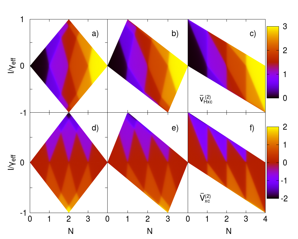
Figure 4: Model Hxc gate (upper panels) and xc bias potentials (lower panels) for a two-level CIM ($\mathcal{M}=2$) according to Eqs. (12a) and (12b), respectively, for different asymmetric coupling at fixed $\gamma=\gamma_{\rm L}+\gamma_{\rm R}$ and $U/\gamma=5$. Panels a) and d): $\gamma_{\rm L}/\gamma=0.5$. Panels b) and e): $\gamma_{\rm L}/\gamma=0.25$. Panels c) and f): $\gamma_{\rm L}/\gamma=5\times 10^{-5}$. Current in units of $\gamma_{\rm eff}=4\gamma_{\rm L}\gamma_{\rm R}/\gamma$, xc potentials in units of $U$.

The model (H)xc potentials of Eq. (12) are constructed by reverse engineering of rate equations. Therefore they contain Coulomb blockade but no Kondo physics. In a DFT framework, the Kondo effect in the zero-bias conductance of weakly coupled quantum dots is already captured correctly in the KS conductance, both for single-level Stefanucci:PRL:2011 ; Bergfield:PRL:2012 ; Troester:PRB:2012 as well as for multi-level dots StefanucciKurth:13 . The incorporation of Kondo physics into the i-DFT functionals thus requires that the derivative of the xc bias w.r.t. the current at $I=0$ vanishes StefanucciKurth:15 . In Ref. Kurth:PRB:2016 we proposed modified (H)xc potentials to include Kondo physics. A further straightforward generalization of these functionals to asymmetric coupling then takes the form (at zero temperature)

$$v^{(\mathcal{M})}_{\rm Hxc,1}[N,I]=(1-a_{1}[I])\bar{v}^{(\mathcal{M})}_{\rm Hxc}[N,I]+a_{1}[I]\bar{v}_{\rm Hxc}[N]$$ (13a)

$$V^{(\mathcal{M})}_{\rm xc,1}[N,I]=(1-a_{1}[I])\bar{V}^{(\mathcal{M})}_{\rm xc}[N,I]\;.$$ (13b)

with the the purely current-dependent function

$$a_{1}[I]=1-\left[\frac{2}{\pi}\arctan\left(\frac{I}{W\gamma_{\rm eff}}\right)\right]^{2}$$ (14)

In Eq. (13a), the zero-current Hxc potential $\bar{v}_{\rm Hxc}$ is defined as $\bar{v}_{\rm Hxc}[N]=\sum_{K=1}^{2{\mathcal{M}-1}}v_{\rm Hxc}^{\rm ext}[N-(K-1)]$ where the extended function is

$$v_{\rm Hxc}^{\rm ext}[N]=\left\{\begin{array}[]{cl}0&\mbox{ $N<0$}\\ v_{\rm Hxc}^{\rm SIAM}[N]&\mbox{ $0\leq N\leq 2$}~{}~{},\\ U&\mbox{ $N>2$}\end{array}\right.$$ (15)

and $v_{\rm Hxc}^{\rm SIAM}[N]$ is the parametrization of the equilibrium SIAM Hxc potential of Ref. Bergfield:PRL:2012 . As a final tweak, we have made the substitution $W\to 2W$ in both $\bar{v}^{(\mathcal{M})}_{\rm Hxc}[N,I]$ and $\bar{V}^{(\mathcal{M})}_{\rm xc}[N,I]$ used in Eqs. (13b). This latter modification has been introduced in Ref. Kurth:PRB:2016 in order to better reproduce accurate differential conductances of the SIAM at symmetric coupling.

In Ref. Jacob:NL:2018 we derived the following exact condition

$$\lim_{\Gamma_{\rm L}\rightarrow 0}v_{\rm Hxc}[n,I](\bm{r})+\frac{1}{2}V_{\rm xc}[n,I]=v_{\rm Hxc}^{(0)}[n](\bm{r})\;.$$ (16)

which relates the (current-dependent) xc gate and bias potentials in the extremely asymmetric limit to the Hxc gate potential in the ground state. The reason we are interested in this particular limit is based on the fact that at zero temperature in this limit and with the bias completely applied to the weakly coupled lead, one can relate the differential conductance to the equilibrium spectral function of the nanoscale region C through Jacob:NL:2018

$$A(\omega)=\lim_{\gamma_{\rm L}\to 0}\frac{4\pi}{\gamma_{\rm eff}}\frac{\partial{I}}{\partial{V}}\bigg{|}_{V=\omega}$$ (17)

where $A(\omega)$ is the trace of the many-body spectral function matrix. Note that $\gamma_{\rm eff}\rightarrow 4\,\gamma_{\rm L}$ for $\gamma_{\rm L}\rightarrow 0$. Computing the differential conductance from i-DFT thus allows to extract the many-body spectral function from a DFT framework.

Unfortunately, our functionals of Eq. (13b) do not satisfy this condition (although the ones of Eq. (12) do). Therefore here we propose an alternative but similar functional for which this condition holds by construction, i.e.,

$$v^{(\mathcal{M})}_{\rm Hxc,2}[N,I] = (1-a_{2}[I])\left(\bar{v}^{(\mathcal{M})}_{\rm Hxc}[N,I]-\bar{v}^{(\mathcal{M})}_{\rm Hxc}[N,0]\right)$$ (18a)

$$+\bar{v}_{\rm Hxc}[N]$$

$$V^{(\mathcal{M})}_{\rm xc,2}[N,I]=(1-a_{2}[I])\bar{V}^{(\mathcal{M})}_{\rm xc}[N,I]\;.$$ (18b)

In principle, in Eq. (18b) we could have used the same function $a_{1}[I]$ (Eq. (14)) as used in the xc potentials of Eq. (13b). However, in order to better reproduce accurate equilibrium spectral functions for the SIAM (in the extremely asymmetric limit), we were compelled to use the alternative function $a_{2}[I]$ as

$$a_{2}[I]=1-\frac{2}{\pi}\arctan\left[\lambda\left(\frac{I}{W\gamma_{\rm eff}}\right)^{2}\right]$$ (19)

where $\lambda=0.16$ is a fit parameter.

3 Results

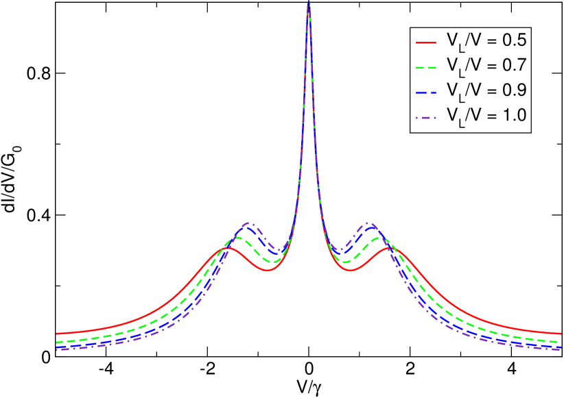
Figure 5: Evolution of the zero-temperature differential conductance of i-DFT using the functional of Eq. (18b) for the symmetrically coupled SIAM with $U/\gamma=3$ at particle-hole symmetry from symmetric to asymmetric voltage drops using the functional of Eq. (18b).

In the present section we will show some results obtained with the functionals described above. Our main focus is on the SIAM which has been studied with many different methods and therefore we can compare the results of our i-DFT approach with accurate reference calculations.

We start with results for the SIAM. As a first example, in Fig. 5 we show how the zero-temperature differential conductance of the symmetrically coupled SIAM at fixed gate $\varepsilon=-U/2$ (particle-hole symmetry) evolves as the bias asymmetry between left and right lead increases. The results were obtained with i-DFT using the functional of Eq. (18b) for interaction strength $U/\gamma=3$. As the asymmetry in the applied bias increases, the side peaks move to lower biases. The Kondo resonance around $V=0$, on the other hand, is not affected by the bias asymmetry.

In Fig. 6 we show the zero-temperature differential conductance of the SIAM for different asymmetry in the coupling to left and right leads obtained with the i-DFT functional of Eq. (18b). Results are shown for two values of the interaction strength, both at particle-hole symmetry and at completely asymmetric voltage drop ($V_{\rm L}=V$). With increasing coupling asymmetry, the maxima of the side peaks decrease significantly and, for $U/\gamma=7.5$, are shifted slightly towards higher biases. For comparison we also show equilibrium spectral functions obtained with Numerical Renormalization Group (NRG) methods Motahari:PRB:2016 . While for the lower interaction strength ($U/\gamma=3$), the i-DFT differential conductance for the highly asymmetrically coupled case $\gamma_{\rm L}/\gamma=10^{-5}$ exhibits side peaks (actually more side shoulders) which agree moderately well with the NRG spectral function, for the higher interaction strength ($U/\gamma=7.5$), the agreement between the i-DFT and NRG spectral functions is actually quite remarkable.

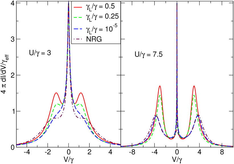
Figure 6: Evolution of the zero-temperature differential conductance of the SIAM from symmetric to completely asymmetric coupling at completely asymmetric voltage drop ($V_{\rm L}=V$) for different interaction strengths $U/\gamma$. In both cases, the external gate is fixed at particle-hole symmetry, $\varepsilon=-U/2$, and the functional of Eq. (18b) has been used. For comparison, equilibrium spectral functions from numerical renormalization group (NRG) calculations of Ref. Motahari:PRB:2016 are shown.

In Fig. 7 we compare the performance of the i-DFT functionals of Eq. (13b) and (18b). In the left panel we compare differential conductances at symmetric coupling and bias for $U/\gamma=3$ at particle-hole symmetry and compare with accurate results from the functional Renormalization Group (fRG) JakobsPletyukhovSchoeller:10 . In the other two panels we compare i-DFT spectral functions (i.e., asymmetric coupling and bias) for $U/\gamma=5$ at (middle panel) and away (right panel) from particle-hole symmetry with NRG results Motahari:PRB:2016 . While for the differential conductance in the symmetrically coupled case, the functional of Eq. (13b) performs somewhat better than the one of Eq. (18b), in the case of the spectral functions the situation is just the opposite. In particular, away from particle-hole symmetry (right panel), the functional (13b) strongly overestimates the side peak for positive frequency while at the same time underestimating the one at negative frequency. Both i-DFT functionals have the tendency to shift the side peaks to lower frequencies. The fact that one of the functionals (Eq. (13b)) performs better for symmetric coupling while the other one (Eq. (18b)) performs better for spectral functions (highly asymmetric coupling and bias) is not really surprising since the corresponding functions $a_{1}[I]$ and $a_{2}[I]$ (Eqs. (14) and (19), respectively) were actually chosen to perform well in exactly the situation where they do. Of course, it would be desirable to have one functional which performs best for all the different situations but so far this has turned out to be elusive. Nevertheless, it is still significant progress that one can obtain from a DFT framework reasonable differential conductances and even (equilibrium) spectral functions for a strongly correlated system like the SIAM.

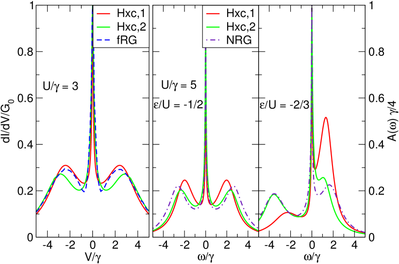
Figure 7: Comparison of the performance of the two different i-DFT functionals of Eq. (13b) and (18b) (denoted as “Hxc,1” and “Hxc,2”, respectively). Left panel: differential conductance of the symmetrically coupled and symmetrically biased SIAM for $U/\gamma=3$ compared to results obtained with the functional renormalization group (fRG) JakobsPletyukhovSchoeller:10 . Middle and right panels: spectral functions for $U/\gamma=5$ at (middle panel) and away from (right panel) ph symmetry. NRG results from Ref. Motahari:PRB:2016 for comparison.

In Fig. 8 we show i-DFT results for differential conductances (normalized by a factor $4\pi/\gamma_{\rm eff}$ of a CIM with $\mathcal{M}=2$ degenerate single-particle levels at completely asymmetrically applied bias and a various asymmetric couplings. Here we have used the functional of Eq. (12) (see also Fig. 4) which includes Coulomb blockade but no Kondo physics. At particle-hole symmetry (left panel) the normalized differential conductances for different coupling asymmetries are qualitatively similar although the height of the Coulomb blockade sidepeaks decreases with increasing coupling asymmetry. On the other hand, the normalized differential conductance at zero bias is independent of the coupling asymmetry, since it is determined by the equilibrium spectral density at the Fermi level, which only depends on the total broadening $\gamma_{\rm L}+\gamma_{\rm R}$. Away from particle-hole symmetry (right panel) the normalized differential conductances also qualitatively changes with increasing coupling asymmetry: while for symmetric coupling ($\gamma_{\rm L}/\gamma=0.5$) we have a three-peak structure in the $\partial{I}/\partial{V}$, in the highly asymmetric case ($\gamma_{\rm L}/\gamma=10^{-5}$) this has been transformed into a two-peak structure. The latter fact is not surprising: for the highly asymmetric limit the density is essentially independent of the bias and, for fixed density, the corresponding xc bias exhibits exactly two steps as the current is varied (see panel f) of Fig. 4). These steps are the origin of the peaks in the differential conductance.

It is worth pointing out that the apparent discontinuities in the differential conductances at zero bias and away from particle-hole symmetry are an artefact of our parametrization, Eq. (12), where the $\Delta^{(\pm)}_{K}(N,I)$ are approximated as piecewise linear functions of $N$ and $I$. As one can appreciate in Fig. 4, these lines (the positions of the steps in the Hxc gate and xc bias) in most cases have kinks when crossing one of the vertices in the $N$-$I$ plane. These kinks are the origin of the discontinuities in the $\partial{I}/\partial{V}$ curves. Therefore, if one parametrized the $\Delta^{(\pm)}_{K}(N,I)$ as differentiable functions of $N$ and $I$ these discontinuities would disappear.

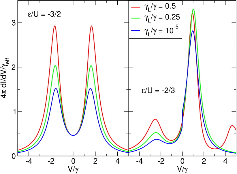
Figure 8: Differential conductance for a degenerate two-level CIM with $U/\gamma=3$ for completely asymmetric bias and different asymmetric couplings obtained with the functional of Eq. (12) at (left panel) and away from particle-hole symmetry (right panel).

4 Conclusions

The recently proposed i-DFT approach provides a promising framework for the DFT description of steady-state transport for both weakly and strongly correlated systems. As usual for any DFT, the crucial ingredient for a successful application is the quality of the approximations for the exchange-correlation functionals. In previous work, functionals have been constructed for the Anderson model and the Constant Interaction Model for the situation when the coupling to the leads is either symmetric or for the limiting case when one of the leads is extremely weakly coupled. In the present work we have generalized these functionals to arbitrary asymmetry and compared their relative performance. This has been achieved by first constructing a functional which is able to capture Coulomb blockade at arbitrary coupling and bias using insights gained from reverse engineering of the rate equation approach. As a second step, Kondo physics can be introduced into the i-DFT functionals in a relatively easy manner by the requirement that the derivative of the xc bias with respect to the current vanishes in the zero-current limit which we have done in two different ways.

In the present as well as in previous work, the i-DFT formalism has been applied to (minimal) model systems describing transport through correlated systems. However, typically one thinks of DFT as a method for an atomistic description of molecular or solid state systems. It is therefore one of the pending tasks of i-DFT to translate the insights gained for model systems into workable approximations which can be applied to an atomistic description of electronic transport.

References

- (1) N. Agraït, A. L. Yegati, and J. M. van Ruitenbeek, Phys. Rep. 377, 81 (2003).
- (2) D. Goldhaber-Gordon et al., Nature 391, 156 (1998).
- (3) J. Park et al., Nature 417, 722 (2002).
- (4) H. Grabert and M. H. Devoret, Single Charge Tunneling, Plenum Press, New York, 1992.
- (5) A. R. Champagne, A. N. Pasupathy, and D. C. Ralph, Nano Lett. 5, 305 (2005).
- (6) V. Madhavan, W. Chen, T. Jamneala, M. F. Crommie, and N. S. Wingreen, Science 280, 567 (1998).
- (7) J. Li, W.-D. Schneider, R. Berndt, and B. Delley, Phys. Rev. Lett. 80, 2893 (1998).
- (8) N. Knorr, M. A. Schneider, L. Diekhöner, P. Wahl, and K. Kern, Phys. Rev. Lett. 88, 096804 (2002).
- (9) A. Zhao et al., Science 309, 1542 (2005).
- (10) V. Iancu, A. Deshpande, and S.-W. Hla, Nano Lett. 6, 820 (2006).
- (11) C. F. Hirjibehedin et al., Science 317, 1199–1203 (2007).
- (12) J. J. Parks et al., Science 328, 1370 (2010).
- (13) J. C. Oberg et al., Nat. Nanotechnol. 9, 64 (2014).
- (14) S. Karan et al., Nano Lett. 18, 88 (2018).
- (15) B. C. Stipe, M. A. Rezaei, and W. Ho, Science 280, 1732 (1998).
- (16) J. R. Hahn, H. J. Lee, and W. Ho, Phys. Rev. Lett. 85, 1914 (2000).
- (17) N. D. Lang, Phys. Rev. B 52, 5335 (1995).
- (18) R. Landauer, IBM J. Res. Develop. 1, 233 (1957).
- (19) M. Büttiker, Phys. Rev. Lett. 57, 1761 (1986).
- (20) G. Stefanucci and S. Kurth, Nano Lett. 15, 8020 (2015).
- (21) G. Stefanucci and S. Kurth, Phys. Rev. Lett. 107, 216401 (2011).
- (22) J. P. Bergfield, Z.-F. Liu, K. Burke, and C. A. Stafford, Phys. Rev. Lett. 108, 066801 (2012).
- (23) P. Tröster, P. Schmitteckert, and F. Evers, Phys. Rev. B 85, 115409 (2012).
- (24) D. Jacob, J. Phys. Condens. Mat. 27, 245606 (2015).
- (25) A. Droghetti and I. Rungger, Phys. Rev. B 95, 085131 (2017).
- (26) E. Runge and E.K.U. Gross, Phys. Rev. Lett. 52, 997 (1984).
- (27) G. Stefanucci and C.-O. Almbladh, EPL (Europhysics Letters) 67, 14 (2004).
- (28) F. Evers, F. Weigend, and M. Koentopp, Phys. Rev. B 69, 235411 (2004).
- (29) M. Koentopp, K. Burke, and F. Evers, Phys. Rev. B 73, 121403 (2006).
- (30) G. Stefanucci, S. Kurth, E. K. U. Gross, and A. Rubio, Theor. Comput. Chem. 17, 247 (2007).
- (31) S. Kurth and G. Stefanucci, Phys. Rev. B 94, 241103 (2016).
- (32) S. Kurth and G. Stefanucci, J. Phys. Condens. Mat. 29, 413002 (2017).
- (33) D. Jacob and S. Kurth, Nano Lett. 18, 2086 (2018).
- (34) S. Kurth and G. Stefanucci, J. Phys.: Condens. Matter 29, 413002 (2017).
- (35) P. W. Anderson, Phys. Rev. 124, 41 (1961).
- (36) C. W. J. Beenakker, Phys. Rev. B 44, 1646 (1991).
- (37) G. Stefanucci and S. Kurth, Phys. Stat. Sol. (b) 250, 2378 (2013).
- (38) S. Motahari, R. Requist, and D. Jacob, Phys. Rev. B 94, 235133 (2016).
- (39) S. G. Jakobs, M. Pletyukhov, and H. Schoeller, Phys. Rev. B 81, 195109 (2010).