Optimal control of light propagation and exciton transfer in arrays of molecular-like noble-metal clusters

Abstract

We demonstrate theoretically the possibility of optimal control of light propagation in arrays constructed of sub-nanometer sized noble metal clusters by using phase-shaped laser pulses and analyze the mechanism underlying this process. The theoretical approach for simulation of light propagation in the arrays is based on the numerical solution of the coupled time-dependent Schrödinger equation and the classical electric field propagation in an iterative self-consistent manner. The electronic eigenstates of individual clusters and the dipole couplings are obtained from ab initio TDDFT calculations. The total electric field is propagated along the array by coupling an external excitation electric field with the electric fields produced by all clusters. A genetic algorithm is used to determine optimal pulse shapes which drive the excitation in a desired direction. The described theoretical approach is applied to control of the light propagation in a T-shaped structure built of seven Ag₈ clusters. We demonstrate that a selective switching of light localization is possible in $\sim$ 5 nm sized cluster arrays which might serve as building block for novel plasmonic devices with ultrafast operation regime.

I Introduction

Since decades noble metal nanoclusters have been attracting scientists by imposing new interesting questions for fundamental research as well as by promising novel opportunities for applications in nanotechnology (Sanchez et al., 1999; Shipway et al., 2000; Bonavci’c-Kouteck’y et al., 2001; Peyser et al., 2001; Zheng et al., 2004; Lal et al., 2007; Johnson et al., 2009; Benson, 2011; Lang and Bernhardt, 2012). The possible fields of applications of noble metal nanoclusters and their assemblies being developed nowadays range from single-molecule probing (Seydack, 2005; Anker et al., 2008) and medical diagnostics (Haes and Van Duyne, 2004; Hahn et al., 2011; Sailor and Park, 2012) to nonlinear light sources (Zheng et al., 2004; Li et al., 2009; Lisinetskaya and Mitri’c, 2011; Polyushkin et al., 2014) and energy transport (Quinten et al., 1998; Maier et al., 2001, 2003; Palacios et al., 2014). A great deal of attention of the researchers working in this field is paid to noble metal nanoparticles with sizes ranging form tens to several hundreds of nanometers. These particles exhibit strong absorption of light mainly in the visible region due to collective excitation of conduction electrons, known as plasmons (Link and El-Sayed, 1999; Jensen et al., 2000), which is absent in the corresponding bulk materials. The energy of plasmon excitation strongly depends on shape, size and dielectric surrounding of nanoparticles or their aggregates (Kelly et al., 2003; Jain et al., 2006), which opens up a fascinating opportunity to tune the light absorption by adjusting these parameters. Along with that, the strong near-field of the nanoparticle can enhance the optical response of a molecule at its vicinity (Nie and Emory, 1997; Tam et al., 2007) or excite neighboring nanoparticles, leading to energy transport (Maier et al., 2001).

The challenging problem of delivering excitation to a desired spatial point at a desired instant of time using noble metal nanoparticles and their aggregates has been recently addressed both experimentally and theoretically, providing impressive and promising results. Using phase modulation of the exciting laser pulse, the possibility of coherent control of ultrafast energy localization in nanostructures has been theoretically demonstrated (Stockman et al., 2002). Optical near field manipulation on a sub-diffraction length scale and on a sub-picosecond time scale has been experimentally achieved in specifically designed aggregates constructed of silver nanoparticles via excitation by polarization-shaped laser pulses designed using adaptive control techniques (Brixner et al., 2005; Aeschlimann et al., 2010). Along with localization of excitation, possibilities of control of light propagation in nanoparticle arrays has been demonstrated both by theory (Sukharev and Seideman, 2006, 2007; Tuchscherer et al., 2009) and experiment (Aeschlimann et al., 2007).

Aiming to further reduce the size of possible nanooptical devices one ultimately reaches the size regime where each atom of a nanoparticle counts. In this size range the plasmonic absorption band transforms into molecular-like discrete energy levels which strongly depend on the number of atoms in the cluster and their geometric structure (Zheng et al., 2004; Morton et al., 2011). Such small particles possess properties which do not scale with the cluster’s size and are considerably different from conventional nanoparticles as well as from corresponding bulk materials (Bonavci’c-Kouteck’y et al., 2001; Mitri’c et al., 2001; Bonavci’c-Kouteck’y et al., 2002; Ma et al., 2012; Stanzel et al., 2012). This makes the molecular-like noble metal clusters promising building blocks for ultra-small optical devices.

Energy localization and light propagation processes in aggregates of the sub-nanometer noble metal clusters are, at the moment, not studied so intensively as in case of their bigger counterparts. The theoretical methods such as the finite-difference time-domain method (FDTD) (Maier et al., 2003; Sukharev and Seideman, 2006), the extended Mie theory (Muehlig et al., 2011; Rockstuhl et al., 2011; Willingham and Link, 2011; Solis et al., 2012; Muehlig et al., 2013), the discrete-dipole approximation (DDA) (Wang and Zou, 2009), the boundary elements method (BEM) (Brixner et al., 2005), and the quasi-static approximation to Maxwell’s equations (Stockman et al., 2004) which are successful in describing 10-100 nm sized nanoparticles, cannot be straightforwardly applied to sub-nanometer clusters due to the small sizes and the intrinsic quantum nature of the latter. Coupling of these methods to the Bloch (Ziolkowski et al., 1995; Fratalocchi et al., 2008), Schrödinger (Lopata and Neuhauser, 2009), and Liouville (Sukharev and Nitzan, 2011) equations allowed for inclusion of quantum effects and description of atomic systems interacting with light. Within these approaches atoms are usually treated as two-, three-, or four-level quantum systems with degenerate excited states. Unfortunately, these methods are not sufficient to describe the electronic structure of a noble metal nanocluster realistically and to simulate the interaction of cluster aggregates with light, which is essential for interpretation of experimental results and design of novel nanosystems.

Recently, we have proposed a method to describe light propagation in arrays consisting of small noble metal clusters (Lisinetskaya and Mitri’c, 2014). The method is based on numerical integration of the time-dependent Schrödinger equations (TDSE) in the manifold of electronic eigenstates of each separate cluster under the action of an external laser field as well as the electric field produced by the other clusters in the array. The TDSE is solved in a self-consistent iterative manner until the convergence of time-dependent dipole moments of all clusters is reached. The results provided by this method have been tested against quantum-mechanical calculations and good agreement has been demonstrated provided the distance between the clusters in the array is large enough.

In the current contribution, we combine the previously introduced theoretical approach (Lisinetskaya and Mitri’c, 2014) with the optimal control employing a genetic algorithm to design phase-shaped laser pulses which drive selectively the excitation to a selected branch of a model T-shaped structure constructed of atomic silver clusters. We simulate the spatio-temporal distribution of the electric field produced by the structure under the action of optimal laser pulses. Analysis of single cluster electron population dynamics allows for describing the mechanism which governs the excitation transfer in the selected direction.

The paper is structured as follows: In Sec. II the theoretical approach is briefly outlined. The results are presented and discussed in Sec. III, and in Sec. IV the conclusions and outlook are given.

II Theory

II.1 Simulation of light propagation

We consider here arrays consisting of $N$ metal clusters with their charge centers placed at positions $\mathbf{R}_{I}$. We assume that the distance between the clusters is large enough to use the dipole-dipole approximation for modeling the cluster-cluster interaction and to neglect the possibility of charge transfer between the clusters. These approximations have been critically examined and justified in our previous work (Lisinetskaya and Mitri’c, 2014) (additionally, see the Supplemental Material (Lisinetskaya and Mitri’c, 2014)). Within this approach, the Hamiltonian operator of the $I$-th cluster can be written in the following way:

$$\mathrm{H}_{I}=\mathrm{H}_{I}^{0}-\boldsymbol{\mu}_{I}\cdot\left(\underset{{\scriptscriptstyle J\neq I}}{\sum}\boldsymbol{\boldsymbol{\varepsilon}}_{J}\left(\mathbf{r},t\right)+\boldsymbol{\boldsymbol{\varepsilon}}_{ext}\left(\mathbf{r},t\right)\right).$$ (1)

Here, $\mathrm{H}_{I}^{0}$ is the field-free electronic Hamiltonian of the $I$-th cluster, $\boldsymbol{\mu}_{I}$ is the electronic dipole moment operator of the cluster, $\boldsymbol{\boldsymbol{\varepsilon}}_{ext}\left(\mathbf{r},t\right)$ is the external electric field strength and $\boldsymbol{\boldsymbol{\varepsilon}}_{J}\left(\mathbf{r},t\right)$ is the electric field produced by the electromagnetic response of the $J$-th cluster in the array. In this Hamiltonian, the term $-\boldsymbol{\mu}_{I}\cdot\underset{{\scriptscriptstyle J\neq I}}{\sum}\boldsymbol{\boldsymbol{\varepsilon}}_{J}\left(\mathbf{r},t\right)$ represents the cluster-cluster interaction, which in our approach is assumed to be purely electromagnetic. The term $-\boldsymbol{\mu}_{I}\cdot\boldsymbol{\boldsymbol{\varepsilon}}_{ext}\left(\mathbf{r},t\right)$ describes the interaction with an external laser field.

In the described approach, we consider metal clusters of arbitrary shape and size, with the only restriction that the individual components are much smaller than the wavelength of the light used for excitation, typically in a low nanometer size range. This allows us to consider the external field to be uniform over the extent of a single cluster and to represent each individual component as a dipole emitter. Thus the terms in the Hamiltonian (1) can be further reduced to $-\boldsymbol{\mu}_{I}\cdot\boldsymbol{\boldsymbol{\varepsilon}}_{ext}\left(\mathbf{R}_{I},t\right)$ for the interaction with the external field and $-\boldsymbol{\mu}_{I}\cdot\boldsymbol{\boldsymbol{\varepsilon}}_{J}(\mathbf{R}_{I},t)$ for the cluster-cluster interaction.

Employing these ingredients, the Hamiltonian of the whole cluster array can be constructed, and the electromagnetic response can be accurately simulated (Lisinetskaya and Mitri’c, 2014). The major obstacle is the size of the Hamiltonian matrix of the whole array, which grows exponentially with the number of clusters, thus making the calculations cumbersome if a sufficient number of electronic states needs to be included. To overcome this difficulty, an iterative approach to describe electron dynamics in such systems has been developed, which allows one to perform simulations for relatively large arrays with many electronic states per cluster included. The applicability of this approach to the systems constructed of Ag₈ clusters placed at relatively large distances, as we deal with in the current work, has been demonstrated previously (Lisinetskaya and Mitri’c, 2014). Here, we briefly outline the major steps of this method.

Instead of dealing with the time-dependent wave function describing the time evolution of the whole array, time-dependent wave functions for each single cluster $\left|\Phi_{I}(t)\right\rangle$ are determined separately by solving numerically the TDSE’s with single-cluster Hamiltonian $\mathrm{H}_{I}$ (1). The single-cluster wave function is expanded in the basis spanned by the eigenfunctions $\left|\Psi_{i}^{(I)}\right\rangle$ of the field-free Hamiltonian $\mathrm{H}_{I}^{0}$

$$\left|\Phi_{I}(t)\right\rangle=\underset{{\scriptstyle i}}{\sum}C_{i}^{(I)}(t)e^{-iE_{i}^{(I)}t}\left|\Psi_{i}^{(I)}\right\rangle,$$ (2)

where $E_{i}^{(I)}$ is the $i$-th electronic state energy of the $I$-th cluster and $C_{i}^{(I)}(t)$ is the time-dependent expansion coefficient. The final set of coupled differential equations for the time-dependent expansion coefficients $C_{i}^{(I)}(t)$ for numerical integration reads:

$$\dot{C}_{i}^{(I)}(t)=i\boldsymbol{\boldsymbol{\varepsilon}}_{ext}\left(\mathbf{R}_{I},t\right)\cdot\underset{{\scriptstyle j}}{\sum}C_{j}^{(I)}(t)e^{-i\left(E_{j}^{(I)}-E_{i}^{(I)}\right)t}\boldsymbol{\mu}_{ij}^{(I)}+$$

$$i\underset{{\scriptstyle j}}{\sum}C_{j}^{(I)}(t)e^{-i\left(E_{j}^{(I)}-E_{i}^{(I)}\right)t}\boldsymbol{\mu}_{ij}^{(I)}\cdot\underset{{\scriptstyle J\neq I}}{\sum}\boldsymbol{\boldsymbol{\varepsilon}}_{J}(\mathbf{R}_{I},t).$$ (3)

The essential quantities needed for solving the set of equations 3 are the electronic state energies $E_{i}^{(I)}$ and the transition dipole moments $\boldsymbol{\mu}_{ij}^{(I)}$ between all electronic states included in the simulations. In principle, for molecular-sized clusters, these quantities can be obtained using any ab initio or semiempirical electronic structure method. In the current work we have used the linear response time-dependent density functional theory (TDDFT) due to its efficiency and applicability to relatively large complex systems. While the electronic state energies and transition dipole moments between the ground and excited electronic states can be obtained employing standard TDDFT routines, the construction of full dipole coupling matrix requires an additional approximate procedure presented in detail elsewhere (Werner et al., 2010).

Notably, Eq. (3) contains the electric field $\boldsymbol{\boldsymbol{\varepsilon}}_{J}(\mathbf{R}_{I},t)$ produced by the $J$-th cluster, which can be calculated on the basis of the time-dependent dipole moment of that cluster (Feynman et al., 1963), while the latter can be determined as the expectation value of the respective dipole moment operator.

Thus Eqs. 3 are coupled not only by the explicit presence of the expansion coefficients $C_{i}^{(J)}(t)$, but also by the implicit dependence of the electric field $\boldsymbol{\boldsymbol{\varepsilon}}_{J}(\mathbf{R}_{I},t)$ on these coefficients. Therefore the system of equations (3) has to be solved for all subunits simultaneously in the self-consistent manner.

Consequently, our approach involves the following steps:

(i) In the first step, we determine the initial guess for the expansion coefficients $\left\{C_{i}^{(I)}(t)\right\}_{0}$ by solving the set of Eqs. (3) taking into account interaction with the external electric field only $\left(\boldsymbol{\boldsymbol{\varepsilon}}_{J}(\mathbf{R}_{I},t)=0\right)$.

(ii) The first approximation to the time-dependent dipole moments $\left\{\mathbf{p}_{J}(t)\right\}_{0}$ of all clusters in the array is obtained.

(iii) The response of all clusters is determined by calculating $\left\{\boldsymbol{\boldsymbol{\varepsilon}}_{J}(\mathbf{R}_{I},t)\right\}_{0}$ and used in the set of Eqs. (3) to find the next approximation to the expansion coefficients $\left\{C_{k}^{(I)}(t)\right\}_{1}$.

Steps (ii)-(iii) are repeated until convergence is reached. Since in the simulations the essential quantities are the time-dependent dipole moments, the criterion for convergence is that the difference between the dipole moments obtained in subsequent iterations $i$ and $i+1$ integrated over the whole simulation time $T$ is less than a certain threshold:

$$\delta=\frac{1}{T}\underset{{\scriptstyle{\scriptscriptstyle J}}}{\sum}\underset{{\scriptstyle{\scriptscriptstyle 0}}}{\overset{{\scriptstyle{\scriptscriptstyle T}}}{\int}}\left|\mathbf{p}_{J}^{i+1}(t)-\mathbf{p}_{J}^{i}(t)\right|\mathrm{d}t<\epsilon.$$ (4)

The convergence of the method is usually reached due to the fact that the main contribution to the coupling between the electronic states of a single cluster comes from the external laser field, and the interaction with the electric field produced by other clusters brings only small perturbation. Thus the initial guess obtained in the step (i) is already a good approximation to the final results, which is further corrected by the inclusion of cluster-cluster interactions.

When the calculation converges, the single-cluster time-dependent dipole moments are determined using the expansion coefficients found and the spatial-temporal electric field distribution is calculated according to (Feynman et al., 1963)

$$\mathbf{E}\left(\mathbf{r},t\right)=\underset{{\scriptscriptstyle I}}{\overset{{\scriptscriptstyle N}}{\sum}}\left\{\frac{-1}{r_{I}^{3}}\left[\mathbf{p}_{I}\left(t^{\prime}\right)+\frac{r_{I}}{c}\mathbf{\dot{p}}_{I}\left(t^{\prime}\right)-\frac{3\mathbf{r}_{I}}{r_{I}^{2}}\left(\mathbf{r}_{I}\cdot\left(\mathbf{p}_{I}\left(t^{\prime}\right)+\frac{r_{I}}{c}\mathbf{\dot{p}}_{I}\left(t^{\prime}\right)\right)\right)+\right.\right.$$

$$\left.\left.\frac{1}{c^{2}}\mathbf{r}_{I}\times\left(\mathbf{\ddot{p}}_{I}\left(t^{\prime}\right)\times\mathbf{r}_{I}\right)\right]_{t^{\prime}=t-\frac{r_{I}}{c}}\right\},$$ (5)

where the summation runs over all clusters in the array, $\mathbf{r}_{I}=\mathbf{r}-\mathbf{R}_{I}$ and $r_{I}$ is its absolute value.

II.2 Optimal control of light propagation

The aim of the control simulations is to localize the electric field in a specified time interval around a particular spatial part of the nanostructure. In the present contribution, we wish to control the light propagation and localization in a T-shaped metal cluster array consisting of seven identical Ag₈ clusters placed at 20 a₀ distance between closest neighbors and irradiated by a phase-shaped short laser pulse (see Fig. 1).

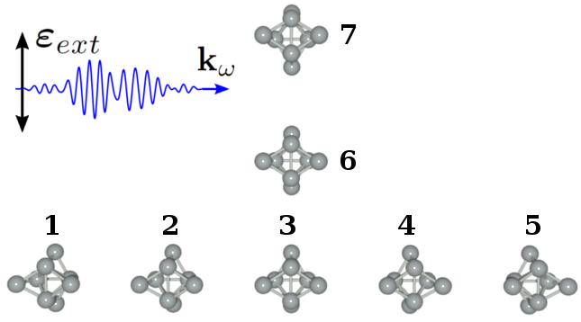
Figure 1: A T-shaped structure consisting of seven Ag₈ clusters placed at 20 a₀ separation irradiated by an external laser pulse $\boldsymbol{\boldsymbol{\varepsilon}}_{ext}\left(\mathbf{r},t\right)$ with the wave vector $\mathbf{k}_{\omega}$.

Thus, as a measure of the spatio-temporal electric field localization we define the following function for each member of the cluster array:

$$W_{I}=\frac{1}{\tau}\underset{{\scriptstyle{\scriptscriptstyle T}-\tau}}{\overset{{\scriptstyle{\scriptscriptstyle T}}}{\int}}\underset{{\scriptstyle{\scriptscriptstyle 0}}}{\overset{{\scriptstyle{\scriptscriptstyle R_{s}}}}{\int}}\underset{{\scriptscriptstyle 4\pi}}{\iint}\left|\mathbf{E}\left(\mathbf{r}^{\prime}+\mathbf{R}_{I},t\right)\right|^{2}\mathrm{d}r^{\prime}\mathrm{d}\Omega\mathrm{d}t,$$ (6)

where $T$ is the simulation time and $\tau$ is the temporal localization interval. The spatial integration is performed within a sphere with the radius $R_{s}$ centered at the specified cluster. In the optimal control simulations we minimize the ratio of the $W$-functions for specified cluster pairs.

A time-dependent phase-shaped external laser pulse is introduced in our model as:

$$\boldsymbol{\boldsymbol{\varepsilon}}_{ext}\left(\mathbf{r},t\right)=\frac{1}{2}\underset{\omega}{\sum}S\left(\omega\right)\left(e^{i\left(\omega t-\mathbf{k}_{\omega}\cdot\mathbf{r}+\varphi\left(\omega\right)\right)}+c.c.\right)\sin^{2}\left(\frac{\pi t}{T_{p}}\right),$$ (7)

where $S\left(\omega\right)$ is the spectrum of the pulse, modeled by a Gaussian function with the mean frequency $\omega_{c}$ and standard deviation $\sigma_{\omega}$

$$S\left(\omega\right)=\frac{1}{\sqrt{2\pi}\sigma_{\omega}}e^{-\frac{\left(\omega-\omega_{c}\right)^{2}}{2\sigma_{\omega}^{2}}},$$ (8)

$\mathbf{k}_{\omega}$ is the wave vector, $\varphi\left(\omega\right)$ is the spectral phase, and the sin²-mask ensures that the pulse fits into the pulse duration period $T_{p}\leq T$. The laser pulse propagates along the long side of the array and is polarized in the plane of the array, as it is shown in Fig. 1. The dependence of the spectral phase on the frequency $\omega$ is determined as follows:

$$\varphi\left(\omega\right)=A\sin\left(B\left(\omega-\omega_{c}\right)+C\left(\omega-\omega_{c}\right)^{2}\right).$$ (9)

Varying the coefficients $A$, $B$, and $C$ one can obtain different temporal profiles of the external laser pulse. In our simulations, we use a genetic algorithm (Goldberg, 1989) to find the proper values $A_{opt}$, $B_{opt}$, and $C_{opt}$ which generate such external pulses that drive the excitation “up” (meaning $W_{7}>W_{5}$) or “straight” ($W_{5}>W_{7}$) after the pulse ceases. Thus the target functions we seek to minimize by means of the genetic algorithm are $f_{1}=W_{5}/W_{7}$ and $f_{2}=W_{7}/W_{5}$. We used population size of 30 “species” and ran the optimization for 30 generations to determine the optimal set of parameters $A_{opt}^{1}$, $B_{opt}^{1}$, and $C_{opt}^{1}$ which minimize $f_{1}$. Afterwards, in the same manner the set of parameters $A_{opt}^{2}$, $B_{opt}^{2}$, and $C_{opt}^{2}$ minimizing $f_{2}$ has been determined.

III Results and discussion

First the equilibrium structure of Ag₈ cluster has been determined by the full geometry optimization in the ground electronic state employing DFT with the gradient corrected Becke-Lee-Yang-Parr (BLYP) exchange-correlation functional (Becke, 1988; Lee et al., 1988), combined with the triple zeta valence plus polarization Gaussian atomic basis set (TZVP) (Schäfer et al., 1994) and a relativistic 19-electron effective core potential for silver (Andrae et al., 1990). Subsequently, a number of excited electronic state energies $E_{i}^{(I)}$ has been calculated employing linear response TDDFT (LR-TDDFT). All calculations have been performed using the TURBOMOLE V.6.3 package (Ahlrichs et al., 1989; Furche and Rappoport, 2005). Then, the transition dipole moments $\boldsymbol{\mu}_{ij}^{(I)}$ between all the electronic states were determined according to Ref. (Werner et al., 2010). The most intense transition in the visible and near-UV range has an excitation energy of 3.8 eV. Therefore the central frequency of the external laser pulse is set to $\omega_{c}$=3.8 eV to be resonant with this intense cluster transition. The parameters $\sigma_{\omega}$ and $T_{p}$ of the external laser pulse as well as other computational details are given in the Supplemental Material (Lisinetskaya and Mitri’c, 2014).

We have performed optimal control simulations with the goal to steer the electric field in two different directions along the T-shaped cluster array shown in Fig. 1. In Fig. 2 we present the dependence of the target function on the generation number showing the convergence of the optimization algorithm. Each point corresponds to the values of the target functions $f_{1}$ and $f_{2}$ defined in Sec. II.2 and averaged over all “species” within this generation. The minimal value of $\left\langle f_{1}\right\rangle$ of 0.57 was obtained in the last generation, while the minimal value of $\left\langle f_{2}\right\rangle$ being equal to 0.63 was obtained in the one-to-last generation. The optimal laser pulse P1 was reconstructed in time domain using Eqs. (7)-(9) with the set of parameters giving rise to the minimal value of $f_{1}$ over all “species” ($A_{opt}^{1}$=6.15, $B_{opt}^{1}$=-16.19 eV^-1, and $C_{opt}^{1}$=-101.79 eV^-2), and for the optimal laser pulse P2 the set of parameters corresponding to the minimal value of $f_{2}$ over all “species” is used ($A_{opt}^{2}$=5.95, $B_{opt}^{2}$=-16.14 eV^-1, and $C_{opt}^{2}$=-18.35 eV^-2).

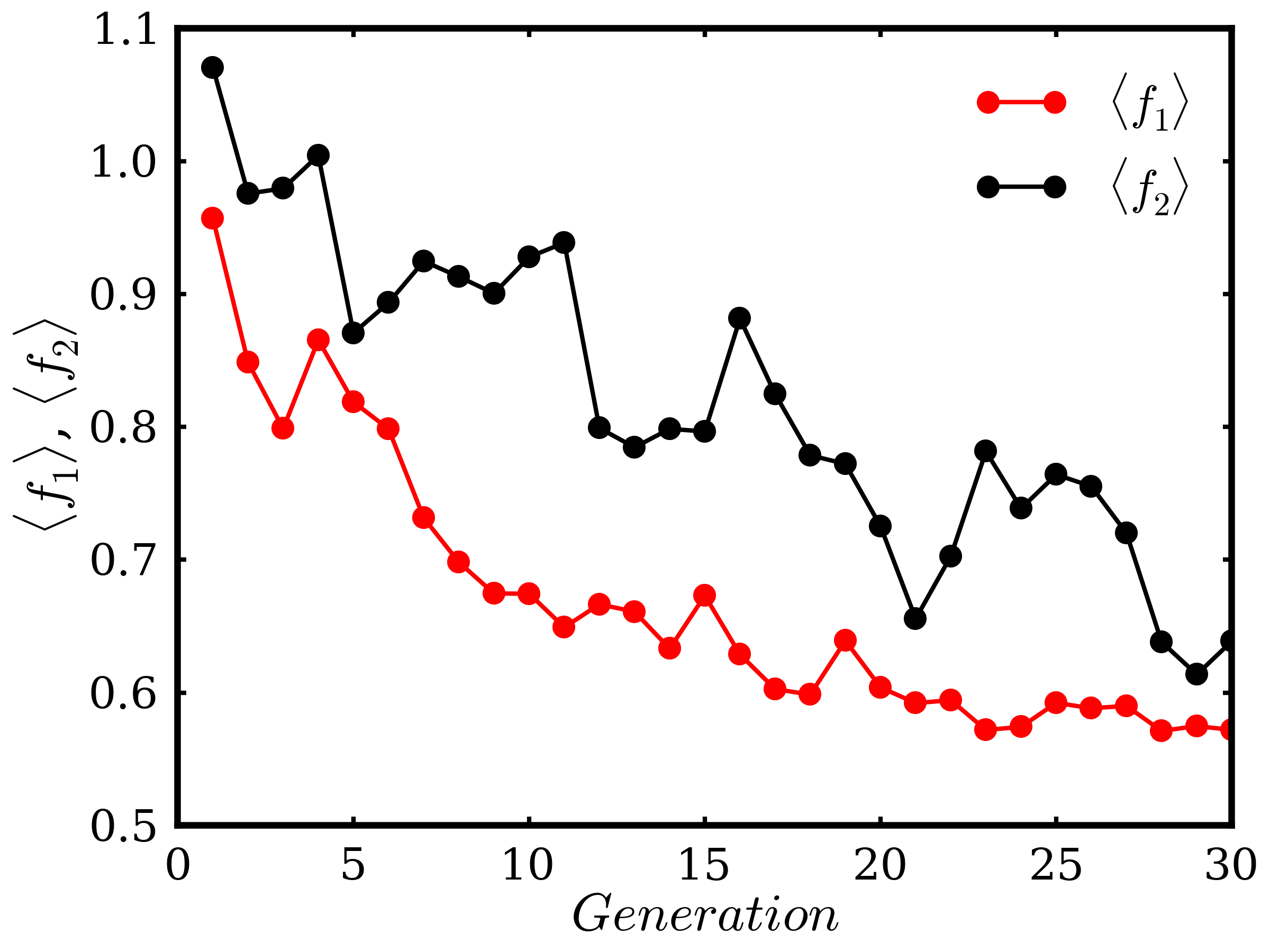
Figure 2: Values of the target functions $f_{1}$ and $f_{2}$ at each generation, averaged over all “species” within this generation.

The electronic state population dynamics of each cluster in the array under the action of the external laser pulse P1 is presented in Fig. 3. The subplots with population dynamics are arranged in order to reproduce the location of the cluster in the array and numbered according to the array scheme shown in the inset (a) for convenience. The temporal profile $\boldsymbol{\boldsymbol{\varepsilon}}\left(t\right)$ of the laser pulse P1 is presented in the inset (b). The ground state population $\left|C_{0}^{(I)}\right|^{2}$ of each single cluster is plotted with the black lines and the populations of the dominantly excited states $\left|C_{17}^{(I)}\right|^{2}$ and $\left|C_{18}^{(I)}\right|^{2}$ is shown with blue and red lines, respectively. Since the latter two states are degenerate and both have nonzero projections of transition dipole moments on the laser pulse polarization vector, both states are populated during the pulse action. It is seen, that at the end of the pulse duration time mainly the ground state of all the clusters is populated, but the last small peak of the laser pulse at $\sim$90 fs (cf. Fig. 3 (b)) causes population transfer to the excited states of the clusters 2, 4, and 6. This increase of population is annotated on Fig. 3 (2,4,6) with black arrows. After the external pulse ceases the electromagnetic interaction between clusters starts to play a decisive role in the population dynamics. The electric field produced by the clusters 2, 4, and 6 is the strongest at the position of the cluster 3, causing the excitation transfer to that cluster. The increase in the excited state population of the cluster 3 is denoted in Fig. 3 (3) with the red arrow. Due to the configuration of the array and the chosen orientation of the clusters, the dipole-dipole interaction between the cluster pair 3-6 is approximately 5 times higher than that between cluster pairs 2-3 and 3-4 in the excited state S₁₈. Therefore, the excitation is propagated “up” along the side chain of the array involving clusters 6 and 7. These steps are denoted in Fig. 3 (6) and (7) with blue and green arrows, respectively. After the excitation reaches the last cluster in the side chain, it is “reflected” back since in our simulations the array is considered to be a closed system.

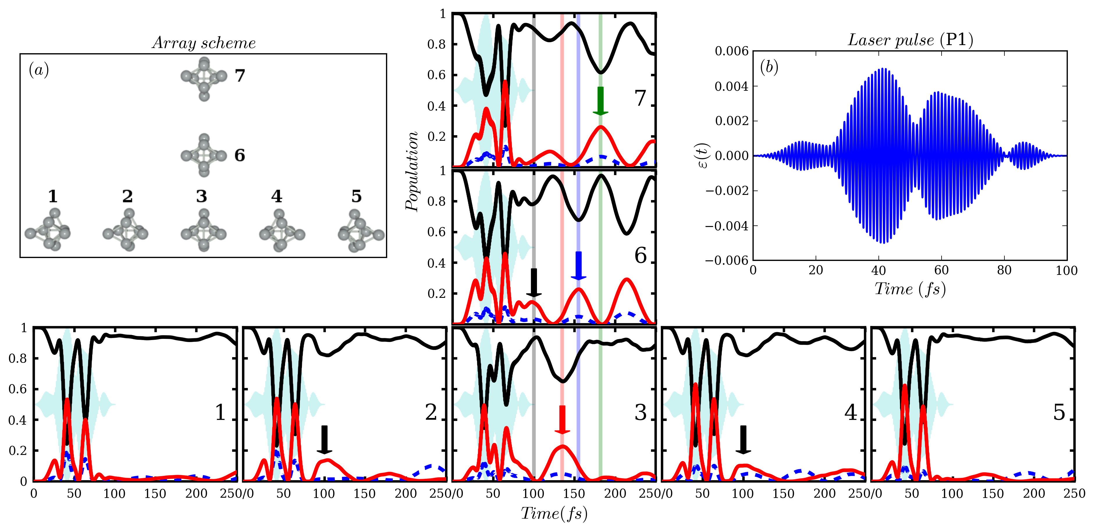
Figure 3: Electron population dynamics of single clusters in the array under the action of the laser pulse P1. Population of the ground state $\left|C_{0}^{(I)}\right|^{2}$ is shown with black lines, of the S₁₇ excited state $\left|C_{17}^{(I)}\right|^{2}$ with blue lines, and of the S₁₈ excited state $\left|C_{18}^{(I)}\right|^{2}$ with red lines. The subplots are arranged and numbered according to the array scheme which is presented in the inset (a). The temporal profile of the external laser pulse P1 is shown in the inset (b). The vertical arrows denote different steps of the excitation propagation “up” along the side chain of the array.

The process of the excitation transfer can be better visualized by simulations of the electric field distribution in the area around the silver cluster array. The electric field strength is determined employing Eq. (5), and the electric field energy density is proportional to the $\left|\mathbf{E}\left(\mathbf{r},t\right)\right|^{2}$. In Fig. 4 the distribution of the electric field $\left|\mathbf{E}\left(\mathbf{r},t\right)\right|^{2}$ at selected instants of time is presented. During the external laser pulse action the electric field varies strongly with time but does not differ much from cluster to cluster, as it is seen for instance at 45 fs of simulation time. When the laser pulse is about to vanish, the electric field around the central clusters of the array is noticeably stronger than around the side clusters. At 100 and 115 fs of the simulation time it is clearly seen how the excitation is transferred from the clusters 2, 4 and 6 to the cluster 3, and afterwards propagates “up” to clusters 6 and 7. At later instants of time the electric field is localized mainly around the top of the array (cluster 7).

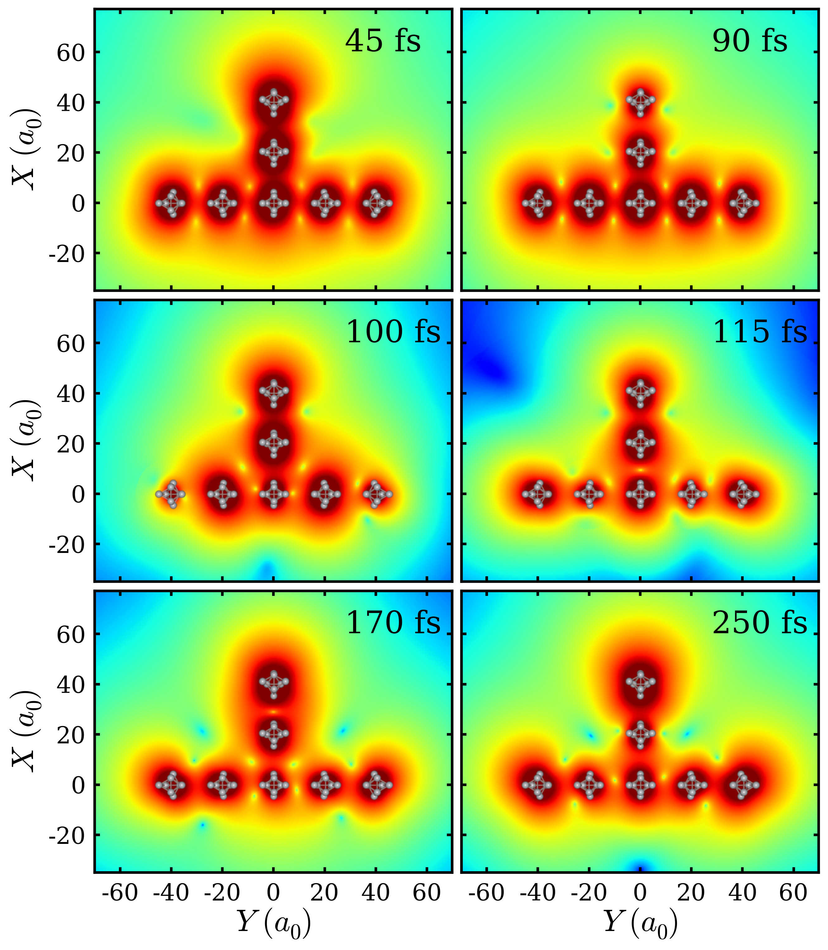
Figure 4: Spatial distribution of the electric field ($\left|\mathbf{E}\left(\mathbf{r},t\right)\right|^{2}$) at selected instants of the simulation time. The snapshots are taken in the plane of the array (XY-plane) at the time moments which are specified in the subplots. The magnitude of the electric field $\left|\mathbf{E}\left(\mathbf{r},t\right)\right|^{2}$ is denoted with the color code from blue (the lowest) to red (the highest).

In the following, we discuss the electron population dynamics of the silver cluster array and the spatio-temporal distribution of the electric field under the action of the second external laser pulse P2, which was optimized to drive the excitation straight along the long side of the array. The electronic state population dynamics of each cluster is presented in Fig. 5. This Figure is arranged in the same way as Fig. 3. The subplots presenting the electron population of the single clusters are placed to resemble the spatial configuration of the silver clusters in the array and the two insets show the array scheme (inset (a)) and the temporal profile of the external pulse (inset (b)). In general, the dipole coupling between the clusters 1-2-3-4-5 forming the horizontal part of the array in the ground and the excited state S₁₈ is considerably smaller than that between clusters 3-6-7 in the side chain, but for the coupling in the excited state S₁₇ the situation is the opposite. Thus to propagate the excitation “straight” along the horizontal side of the array it is required to selectively populate the excited state S₁₇, which is not strongly populated by the external laser pulse due to the small projection of the corresponding transition dipole moment on the polarization direction of the pulse. Consequently, in the optimization procedure, the pulse P2 has been designed, which leads to more complicated electron dynamics as compared to the pulse P1. The action of P2 results in a decrease of the ground state population of the central clusters of the array (2,3,4 and 6) down to 0.5-0.6 (shown in Fig. 5 (3), (6), and (7) with black arrows). After the pulse ceases, due to the strong coupling between the clusters 3 and 6 the excitation is rapidly transferred to the cluster 6, and then some part is further propagated “up” to the cluster 7. However, due to the high electron population in the excited state S₁₈ of the cluster 6, the interaction between clusters 2-6 and 4-6 starts to play a role for transferring the population to the excited states S₁₈ of the cluster 2 as well as S₁₇ and S₁₈ of the cluster 4. This step is marked in Fig. 5 (2), (4), and (7) with red arrows. Finally, part of the excitation mainly from the state S₁₇ of the cluster 4 is propagated “straight” along the long side of the array to the cluster 5 leading to monotonic increase of the electron population of the S₁₈ state . The rest of the excitation is redistributed among the other clusters in this part of the array. This step is annotated in Fig. 5 (2)-(5) with blue arrows.

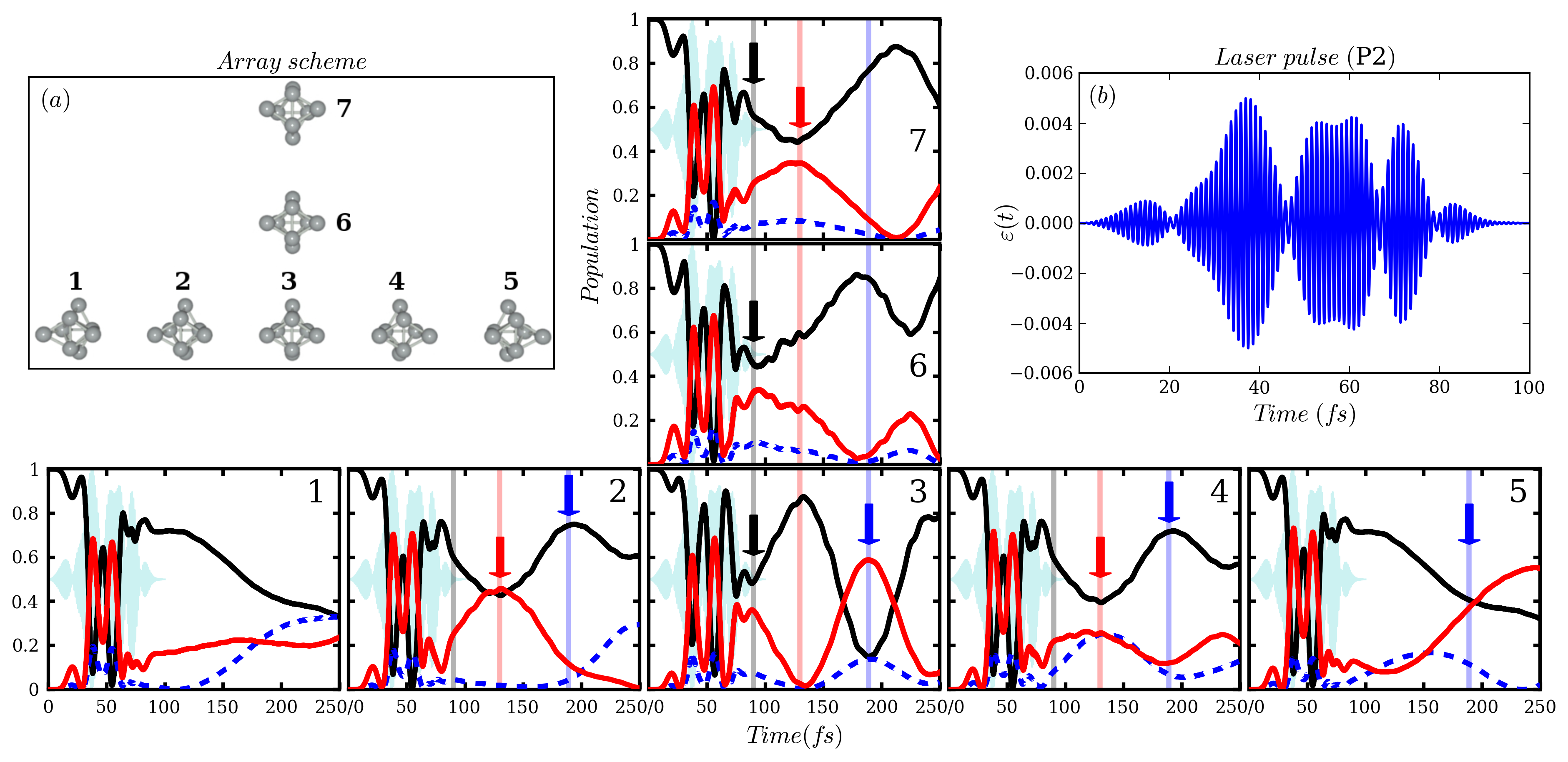
Figure 5: Electron population dynamics of single clusters in the array under the action of the laser pulse P2. Population of the ground state $\left|C_{0}^{(I)}\right|^{2}$ is shown with black lines, of the S₁₇ excited state $\left|C_{17}^{(I)}\right|^{2}$ with blue lines, and of the S₁₈ excited state $\left|C_{18}^{(I)}\right|^{2}$ with red lines. The subplots are arranged and numbered according to the array scheme which is presented in the inset (a). The temporal profile of the external laser pulse P2 is shown in the inset (b). The vertical arrows denote different steps of the excitation propagation “straight” along the horizontal side of the array.

The spatio-temporal variation of the electric field produced by the array is illustrated in Fig. 6. As in the case of P1 excitation, during the pulse action the electric field does not differ much for different clusters. At the end of the excitation time ($\sim$90 fs) the electric field is noticeably stronger in the central part of the array. After the external pulse ceases, the electric field is redistributed around the clusters that form the long side of the array (see Fig. 6 130-230 fs).

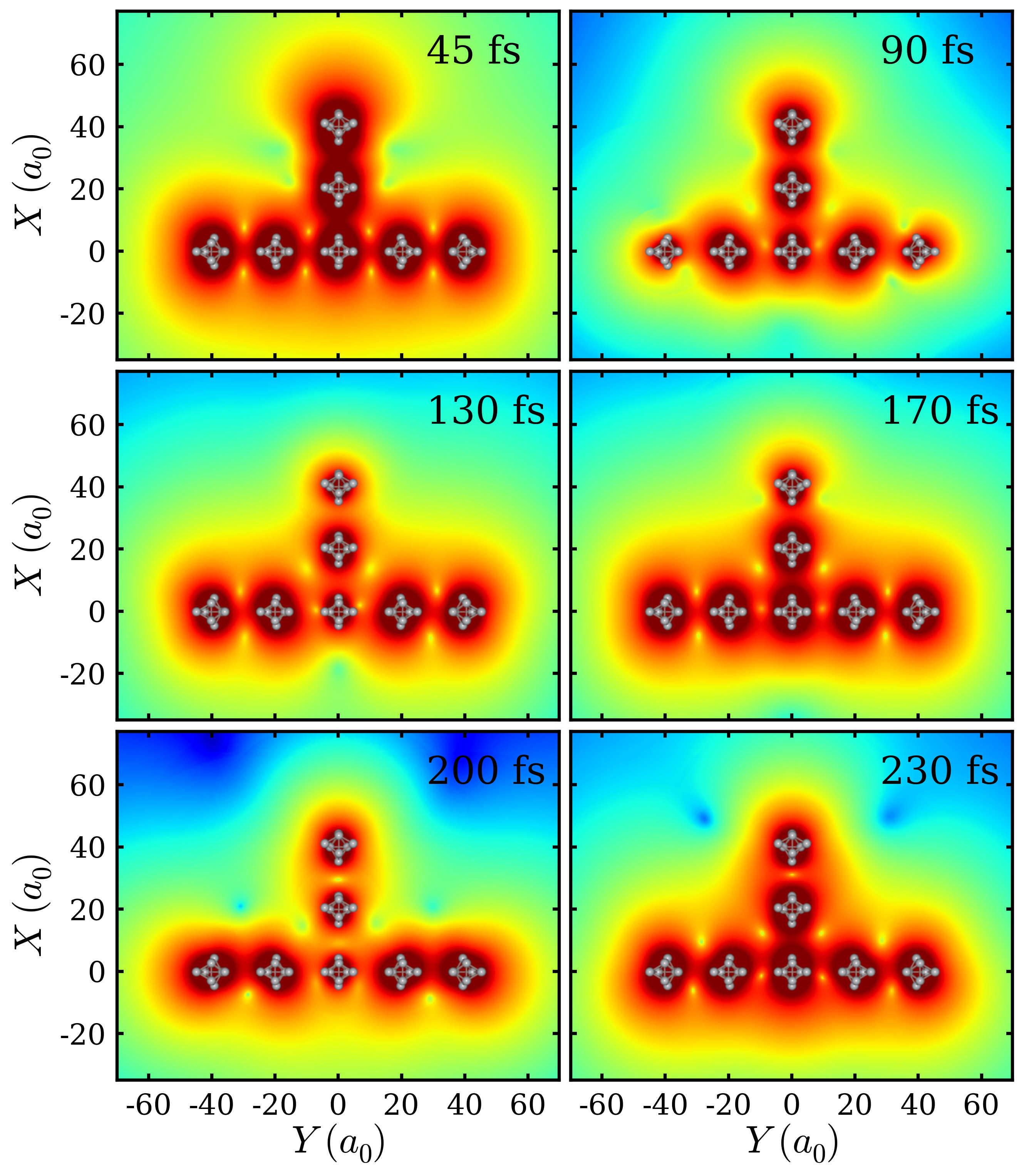
Figure 6: Spatial distribution of the electric field ($\left|\mathbf{E}\left(\mathbf{r},t\right)\right|^{2}$) at selected instants of the simulation time. The snapshots are taken in the plane of the array (XY-plane) at the time moments which are specified in the subplots. The magnitude of the electric field $\left|\mathbf{E}\left(\mathbf{r},t\right)\right|^{2}$ is denoted with the color code from blue (the lowest) to red (the highest).

Finally, we compare the electric field energy around the clusters 5 and 7 along the simulation under the action of pulses P1 and P2. As a measure of the electric field energy we use the functions $W_{5}\left(t\right)$ and $W_{7}\left(t\right)$ calculated using Eq. (6) without integration over time. The results are presented in Fig. 7 (a) for the pulse P1 and (b) for the pulse P2. The time interval $\tau$ within which the energy has been integrated to obtain the target functions $f_{1}$ and $f_{2}$ is shaded on the figures. It is clearly seen in Fig. 7 (a) that within the interval of interest the electric field energy propagated to the “top” of the array (to the cluster 7) significantly exceeds its counterpart localized around cluster 5. In other words, most of the electric field energy is propagated “up” along the side chain of the array. On the other hand, after the action of the pulse P2 the electric field is much stronger around cluster 5 than around cluster 7, i.e. the electric field is propagated “straight” along the long side of the array. This demonstrates that selective switching of the light localization can be achieved by analytically parametrized optimal laser fields, which is of interest for the development of plasmonic nanoelectronic devices with ultrafast optical response.

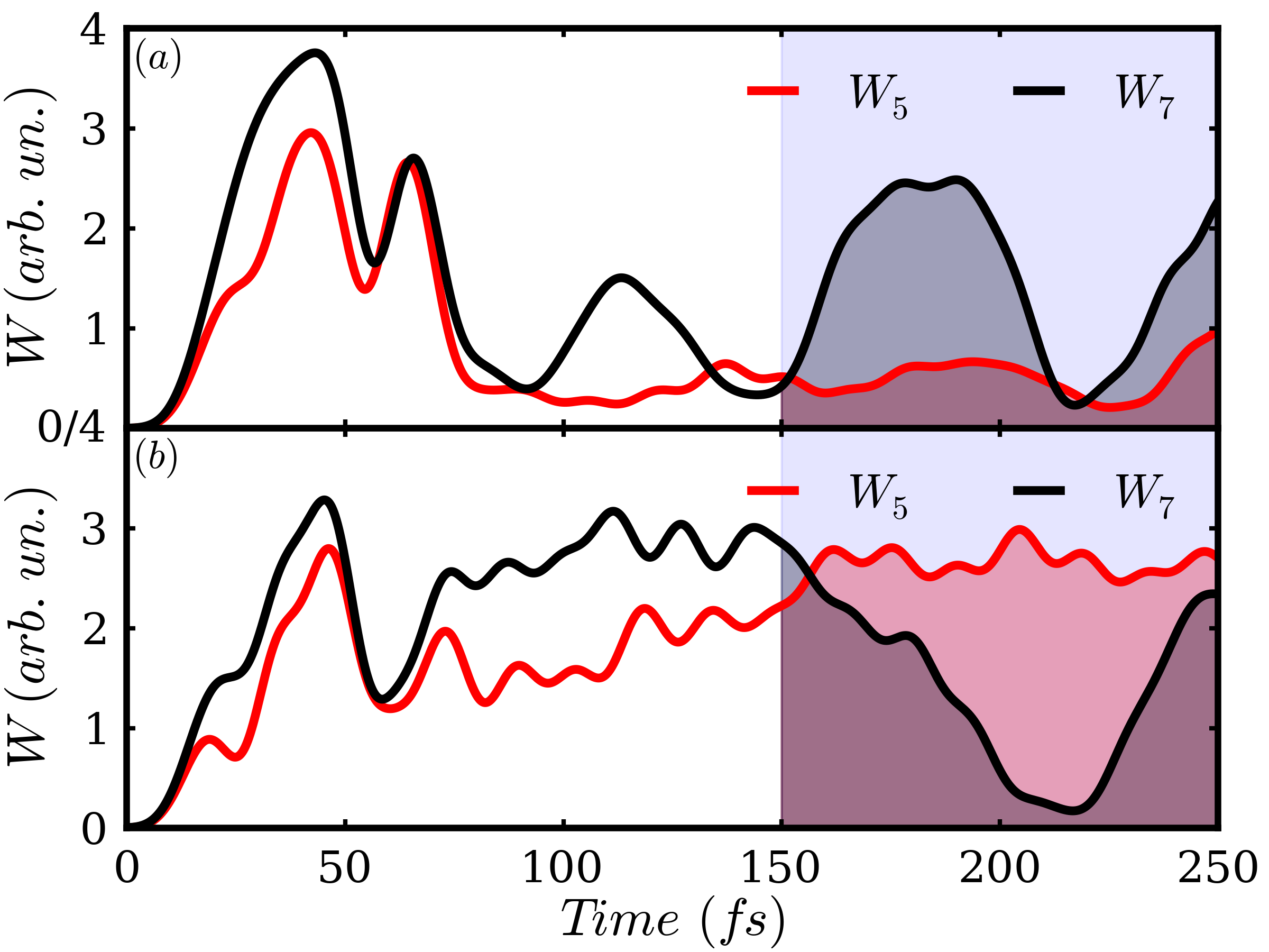
Figure 7: Electric field energies $W_{I}\left(t\right)$ calculated using Eq. (6) for cluster 5 ($W_{5}$) and cluster 7 ($W_{7}$). The results are obtained for the silver cluster array excitation with (a) the laser pulse P1, and (b) the laser pulse P2. The time interval of optimization of the ratio between these energies is shaded in both pictures.

IV Conclusion

We have demonstrated the possibility to optimally control the light propagation in a T-shaped nanostructure built up of small atomic silver clusters. For this purpose we have combined our recently developed iterative method for the simulation of light propagation in metal cluster arrays with the optimal control using a genetic algorithm. The driving field was analytically parametrized in the frequency domain. The ground and excited state energies of individual clusters as well as the transition dipole moments required for the electron dynamics simulation are determined based on ab initio TDDFT calculations, which allowed for a realistic description of the electronic structure of the clusters. We have demonstrated that laser pulses can be designed which selectively drive the electric field either along the main axis of the array or along the side chain. This allows to achieve spatio-temporal electric field localization in different parts of the nanostructure over time intervals of ~ 100 fs. Thus our “proof of principle” simulations demonstrate that nanoelectronic devices build from small noble metal clusters can operate selectively in an ultrafast regime and thus may serve as building blocks for the next generation of nanoplasmonic devices.

References

- Sanchez et al. (1999) Sanchez, A.; Abbet, S.; Heiz, U.; Schneider, W. D.; Hakkinen, H.; Barnett, R. N.; Landman, U. J. Phys. Chem. A 1999, 103, 9573.
- Shipway et al. (2000) Shipway, A. N.; Katz, E.; Willner, I. Chem. Phys. Chem. 2000, 1, 18–52.
- Bonavci’c-Kouteck’y et al. (2001) Bonačić-Koutecký, V.; Veyret, V.; Mitrić, R. J. Chem. Phys. 2001, 115, 10450.
- Peyser et al. (2001) Peyser, L. A.; Vinson, A. E.; Bartko, A. P.; Dickson, R. M. Science 2001, 291, 103.
- Zheng et al. (2004) Zheng, J.; Zhang, C. W.; Dickson, R. M. Phys. Rev. Lett. 2004, 93, 077402.
- Lal et al. (2007) Lal, S.; Link, S.; Halas, N. J. Nat. Photon. 2007, 1, 641–648.
- Johnson et al. (2009) Johnson, G. E.; Mitrić, R.; Bonačić-Koutecký, V.; Castleman, J. A. W. Chem. Phys. Lett. 2009, 475, 1–9.
- Benson (2011) Benson, O. Nature 2011, 480, 193–199.
- Lang and Bernhardt (2012) Lang, S. M.; Bernhardt, T. M. Phys. Chem. Chem. Phys. 2012, 14, 9255–9269.
- Seydack (2005) Seydack, M. Bosensors & Bioelectronics 2005, 20, 2454–2469.
- Anker et al. (2008) Anker, J. N.; Hall, W. P.; Lyandres, O.; Shah, N. C.; Zhao, J.; Van Duyne, R. P. Nature Mater. 2008, 7, 442–453.
- Haes and Van Duyne (2004) Haes, A.; Van Duyne, R. Expert Rev. Mol. Diagn. 2004, 4, 527–537.
- Hahn et al. (2011) Hahn, M. A.; Singh, A. K.; Sharma, P.; Brown, S. C.; Moudgil, B. M. Anal. Bioanal. Chem. 2011, 399, 3–27.
- Sailor and Park (2012) Sailor, M. J.; Park, J.-H. Adv. Mater. 2012, 24, 3779–3802.
- Li et al. (2009) Li, Z.; Shegai, T.; Haran, G.; Xu, H. ACS Nano 2009, 3, 637–642.
- Lisinetskaya and Mitri’c (2011) Lisinetskaya, P. G.; Mitrić, R. Phys. Rev. A 2011, 83, 033408.
- Polyushkin et al. (2014) Polyushkin, D. K.; Marton, I.; Racz, P.; Dombi, P.; Hendry, E.; Barnes, W. L. Phys. Rev. B 2014, 89, 125426.
- Quinten et al. (1998) Quinten, M.; Leitner, A.; Krenn, J. R.; Aussenegg, F. R. Opt. Lett. 1998, 23, 1331–1333.
- Maier et al. (2001) Maier, S. A.; Brongersma, M. L.; Kik, P. G.; Meltzer, S.; Requicha, A. A. G.; Atwater, H. A. Adv. Mater. 2001, 13, 1501–1505.
- Maier et al. (2003) Maier, S. A.; Kik, P. G.; Atwater, H. A. Phys. Rev. B 2003, 67, 205402.
- Palacios et al. (2014) Palacios, E.; Chen, A.; Foley, J.; Gray, S. K.; Welp, U.; Rosenmann, D.; Vlasko-Vlasov, V. K. Adv. Opt. Mater. 2014, 2, 394–399.
- Link and El-Sayed (1999) Link, S.; El-Sayed, M. A. J. Phys. Chem. B 1999, 103, 8410.
- Jensen et al. (2000) Jensen, T. R.; Malinsky, M. D.; Haynes, C. L.; Van Duyne, R. P. J. Phys. Chem. B 2000, 104, 10549–10556.
- Kelly et al. (2003) Kelly, K. L.; Coronado, E.; Zhao, L. L.; Schatz, G. C. J. Phys. Chem. B 2003, 107, 668–677.
- Jain et al. (2006) Jain, P. K.; Lee, K. C.; El-Sayed, I. H.; El-Sayed, M. A. J. Phys. Chem. B 2006, 110, 7238–7248.
- Nie and Emory (1997) Nie, S.; Emory, S. R. Science 1997, 275, 1102–1106.
- Tam et al. (2007) Tam, F.; Goodrich, G. P.; Johnson, B. R.; Halas, N. J. Nano Lett. 2007, 7, 496–501.
- Stockman et al. (2002) Stockman, M. I.; Faleev, S. V.; Bergman, D. J. Phys. Rev. Lett. 2002, 88, 067402.
- Brixner et al. (2005) Brixner, T.; García de Abajo, F. J.; Schneider, J.; Pfeiffer, W. Phys. Rev. Lett. 2005, 95, 093901.
- Aeschlimann et al. (2010) Aeschlimann, M.; Bauer, M.; Bayer, D.; Brixner, T.; Cunovic, S.; Dimler, F.; Fischer, A.; Pfeiffer, W.; Rohmer, M.; Schneider, C.; Steeb, F.; Strueber, C.; Voronine, D. V. Proc. Natl. Acad. Sci. U.S.A. 2010, 107, 5329–5333.
- Sukharev and Seideman (2006) Sukharev, M.; Seideman, T. Nano Letters 2006, 6, 715–719.
- Sukharev and Seideman (2007) Sukharev, M.; Seideman, T. J. Phys. B 2007, 40, S283–S298.
- Tuchscherer et al. (2009) Tuchscherer, P.; Rewitz, C.; Voronine, D. V.; Javier Garcia de Abajo, F.; Pfeiffer, W.; Brixner, T. Opt. Express 2009, 17, 14235–14259.
- Aeschlimann et al. (2007) Aeschlimann, M.; Bauer, M.; Bayer, D.; Brixner, T.; Garcia de Abajo, F. J.; Pfeiffer, W.; Rohmer, M.; Spindler, C.; Steeb, F. Nature 2007, 446, 301–304.
- Morton et al. (2011) Morton, S. M.; Silverstein, D. W.; Jensen, L. Chem. Rev. 2011, 111, 3962–3994.
- Mitri’c et al. (2001) Mitrić, R.; Hartmann, M.; Stanca, B.; Bonačić-Koutecký, V.; Fantucci, P. J. Phys. Chem. A 2001, 105, 8892.
- Bonavci’c-Kouteck’y et al. (2002) Bonačić-Koutecký, V.; Burda, J.; Ge, M.; Mitrić, R.; Zampella, G.; Fantucci, R. J. Chem. Phys. 2002, 117, 3120.
- Ma et al. (2012) Ma, H.; Gao, F.; Liang, W. Z. J. Phys. Chem. C 2012, 116, 1755–1763.
- Stanzel et al. (2012) Stanzel, J.; Neeb, M.; Eberhardt, W.; Lisinetskaya, P. G.; Petersen, J.; Mitric, R. Phys. Rev. A 2012, 85, 013201.
- Muehlig et al. (2011) Muehlig, S.; Cunningham, A.; Scheeler, S.; Pacholski, C.; Buergi, T.; Rockstuhl, C.; Lederer, F. ACS Nano 2011, 5, 6586–6592.
- Rockstuhl et al. (2011) Rockstuhl, C.; Menzel, C.; Muehlig, S.; Petschulat, J.; Helgert, C.; Etrich, C.; Chipouline, A.; Pertsch, T.; Lederer, F. Phys. Rev. B 2011, 83, 245119.
- Willingham and Link (2011) Willingham, B.; Link, S. Opt. Express 2011, 19, 6450–6461.
- Solis et al. (2012) Solis, D.; Willingham, B.; Nauert, S. L.; Slaughter, L. S.; Olson, J.; Swanglap, P.; Paul, A.; Chang, W.-S.; Link, S. Nano Letters 2012, 12, 1349–1353.
- Muehlig et al. (2013) Muehlig, S.; Cunningham, A.; Dintinger, J.; Farhat, M.; Bin Hasan, S.; Scharf, T.; Buergi, T.; Lederer, F.; Rockstuhl, C. Sci. Rep. 2013, 3, 2328.
- Wang and Zou (2009) Wang, H.; Zou, S. Phys. Chem. Chem. Phys. 2009, 11, 5871–5875.
- Stockman et al. (2004) Stockman, M. I.; Bergman, D. J.; Kobayashi, T. Phys. Rev. B 2004, 69, 054202.
- Ziolkowski et al. (1995) Ziolkowski, R.; Arnold, J.; Gogny, D. Phys. Rev. A 1995, 52, 3082–3094.
- Fratalocchi et al. (2008) Fratalocchi, A.; Conti, C.; Ruocco, G. Phys. Rev. A 2008, 78, 013806.
- Lopata and Neuhauser (2009) Lopata, K.; Neuhauser, D. J. Chem. Phys. 2009, 131, 014701.
- Sukharev and Nitzan (2011) Sukharev, M.; Nitzan, A. Phys. Rev. A 2011, 84, 043802.
- Lisinetskaya and Mitri’c (2014) Lisinetskaya, P. G.; Mitrić, R. Phys. Rev. B 2014, 89.
- Lisinetskaya and Mitri’c (2014) See Supplemental Material at http://link.aps.org/supplemental/10.1103/PhysRevB.91.125436 for validation of the interactive method used and further computational details..
- Werner et al. (2010) Werner, U.; Mitrić, R.; Bonačić-Koutecký, V. J. Chem. Phys. 2010, 132, 174301.
- Feynman et al. (1963) Feynman, R. P.; Leighton, R. B.; Sands, M. L. Mainly electromagnetism and matter; The Feynman Lectures on Physics; Addison-Wesley, 1963.
- Goldberg (1989) Goldberg, D. E. Genetic Algorithms in Search, Optimization and Machine Learning; Addison-Wesley, 1989.
- Becke (1988) Becke, A. Phys. Rev. A 1988, 38, 3098–3100.
- Lee et al. (1988) Lee, C.; Yang, W.; Parr, R. Phys. Rev. B 1988, 37, 785–789.
- Schäfer et al. (1994) Schäfer, A.; Huber, C.; R. Ahlrichs, R. J. Chem. Phys. 1994, 100, 5829.
- Andrae et al. (1990) Andrae, D.; Häussermann, U.; Dolg, M.; Preuss, H. Theor. Chem. Acta 1990, 77, 123–141.
- Ahlrichs et al. (1989) Ahlrichs, R.; Bär, M.; Häser, M.; Horn, H.; Kölmel, M. Chem. Phys. Lett. 1989, 162, 165.
- Furche and Rappoport (2005) Furche, F.; Rappoport, D. In Computational Photochemistry; Olivucci, M., Ed.; Theoretical and Computational Chemistry; Elsevier, Amsterdam, 2005; Vol. 16; Chapter 3.