Supplement to “Reduced Basis Kriging for Massive Spatial Fields”

S-1 Additional Experimental Evaluations

A simulation study was conducted to assess the value of reduced basis kriging in comparison to obtaining maximum likelihood estimates of the Spatial Random Effects model via the E-M algorithm. One hundred 2-dimensional Gaussian random fields were simulated using the R package fields (Nychka et al.,, 2015) on either a $50\times 50$ or $200\times 200$ grid. The spatial process at the locations of the observations were assumed to follow a Gaussian distribution with a Matérn covariance structure. The Matérn parameter values $\nu$ and $\theta$ were varied in unison to be such that $(\nu,\theta)\in\{(0.5,0.205),(1,0.137),(1.5,0.110),(2,0.095)\}$, holding $\rho=1$ constant. For each field, simulated measurement errors ($\sigma^{2}=\{0,0.1,0.25,0.4\}$) were added to each response at 300 randomly selected locations, resulting in values that represented data.

ML estimates and the corresponding predicted values for each simulated field were then computed using three different methods: reduced basis kriging using an identity covariance for $\boldsymbol{K}=\delta\boldsymbol{I}$ (blue), by the E-M approach approximating $\boldsymbol{K}$ with the identity matrix, $\delta\boldsymbol{I}$ (gold), and by the E-M approach using the full form of $\boldsymbol{K}$ with constant $b=1.5$ (white). Basis functions with a single resolution and either 23, 77, or 175 knots were used during estimation and prediction, with the bandwidth constant allowed to vary from 0.5 to 2.5 by 0.1 for both methods that use the identity covariance. As mentioned in the full paper, these computations were done using sparse matrix methods (Davis,, 2006) implemented as per the R package “Matrix” (Bates and Maechler,, 2015).

The value of reduced basis kriging was quantified by two summaries: the time required to iterate to convergence followed by computing kriging estimates and the mean square prediction error of the predicted field. The distributions of the one hundred simulated fields are represented with boxplots on the log scale in Figures S-1 through S-16. For clarity of presentation, the distribution of seconds or MSPE for the E-M approach using the full form of $\boldsymbol{K}$ are truncated on the main figure and presented in full separately when the maximum is significantly beyond the range of the corresponding results for the identity form of $\boldsymbol{K}$, as in Figure S-1(c).

Two expected gains in computational efficiency were achieved by either using the identity covariance for $\boldsymbol{K}$ or by using fewer knots. The value of the bandwidth constant, $b$, was also critical to minimizing CPU time because it controlled the level of sparsity in $\boldsymbol{S}$. The effect of $b$ on the E-M approach was predictable as lower values resulted in decreased CPU time, with an optimal level of sparsity occurring near $b=1$ for the $50\times 50$ grid. An interesting difference between the E-M approach and reduced basis kriging is the robustness of reduced basis kriging to increasing $m$ or a poor choice of bandwidth constant. Reduced basis kriging is efficient regardless of the specifics of the basis functions used and is at least as efficient as the E-M approach with the identity covariance for any reasonable choice of $b$. The E-M approach is consistently more computationally expensive for larger values of $b$. When the $200\times 200$ grid size was used, the E-M approach would occasionally reach convergence sooner than reduced basis kriging for low values of the bandwidth constant ($b<1$), with a dramatic reduction occurring when $b=0.5$ and $m=23$. However, the resulting MSPE of these estimations were particularly poor.

The distributions of MSPE for both $50\times 50$ and $200\times 200$ grid sizes show that for a reasonable $b$, the identity covariance structure is at least as accurate in terms of prediction as the full covariance structure. In fact, as $m$ approaches $n$, the identity covariance performs substantially better than the full covariance with regards to both median and maximum MSPE. This suggests that added complexity to $\boldsymbol{K}$ is unnecessary when our focus is on prediction. Using the identity covariance for $\boldsymbol{K}$, reduced basis kriging and the E-M approach are comparable for choices of bandwidth constant where MSPE is minimized, however an unreasonable $b$ favors the E-M approach in terms of MSPE. This is opposite of computational efficiency, in which reduced basis kriging was more robust to poor choices of $b$.

(a) $50\times 50$ grid with $m=23$

(b) $50\times 50$ grid with $m=23$

(c) $50\times 50$ grid with $m=77$

(d) $50\times 50$ grid with $m=77$

(e) $50\times 50$ grid with $m=175$

(f) $50\times 50$ grid with $m=175$

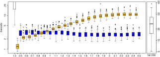
(g) $200\times 200$ grid with $m=23$

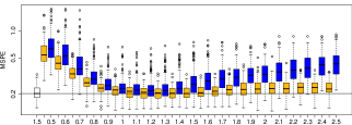
(h) $200\times 200$ grid with $m=23$

(i) $200\times 200$ grid with $m=77$

(j) $200\times 200$ grid with $m=77$

(k) $200\times 200$ grid with $m=175$

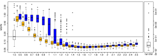
(l) $200\times 200$ grid with $m=175$

Figure S-1: Seconds (left panel) and Mean Squared Prediction Errors (MSPEs, right panel) for varying bandwidths constants (x-axis) and number of knots ($m$) for all three estimation methods on both grids when $\nu=0.5$ and $\sigma^{2}=0$.

(a) $50\times 50$ grid with $m=23$

(b) $50\times 50$ grid with $m=23$

(c) $50\times 50$ grid with $m=77$

(d) $50\times 50$ grid with $m=77$

(e) $50\times 50$ grid with $m=175$

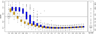
(f) $50\times 50$ grid with $m=175$

(g) $200\times 200$ grid with $m=23$

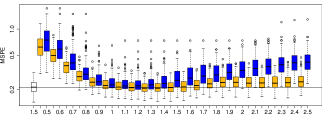
(h) $200\times 200$ grid with $m=23$

(i) $200\times 200$ grid with $m=77$

(j) $200\times 200$ grid with $m=77$

(k) $200\times 200$ grid with $m=175$

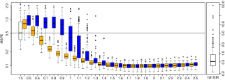
(l) $200\times 200$ grid with $m=175$

Figure S-2: Seconds (left panel) and Mean Squared Prediction Errors (MSPEs, right panel) for varying bandwidths constants (x-axis) and number of knots ($m$) for all three estimation methods on both grids when $\nu=0.5$ and $\sigma^{2}=0.1$.

(a) $50\times 50$ grid with $m=23$

(b) $50\times 50$ grid with $m=23$

(c) $50\times 50$ grid with $m=77$

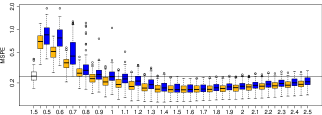
(d) $50\times 50$ grid with $m=77$

(e) $50\times 50$ grid with $m=175$

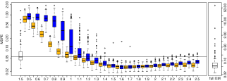
(f) $50\times 50$ grid with $m=175$

(g) $200\times 200$ grid with $m=23$

(h) $200\times 200$ grid with $m=23$

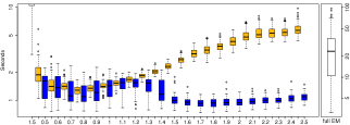
(i) $200\times 200$ grid with $m=77$

(j) $200\times 200$ grid with $m=77$

(k) $200\times 200$ grid with $m=175$

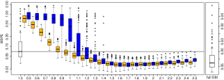
(l) $200\times 200$ grid with $m=175$

Figure S-3: Seconds (left panel) and Mean Squared Prediction Errors (MSPEs, right panel) for varying bandwidths constants (x-axis) and number of knots ($m$) for all three estimation methods on both grids when $\nu=0.5$ and $\sigma^{2}=0.25$.

(a) $50\times 50$ grid with $m=23$

(b) $50\times 50$ grid with $m=23$

(c) $50\times 50$ grid with $m=77$

(d) $50\times 50$ grid with $m=77$

(e) $50\times 50$ grid with $m=175$

(f) $50\times 50$ grid with $m=175$

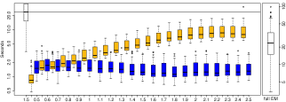
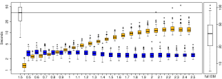
(g) $200\times 200$ grid with $m=23$

(h) $200\times 200$ grid with $m=23$

(i) $200\times 200$ grid with $m=77$

(j) $200\times 200$ grid with $m=77$

(k) $200\times 200$ grid with $m=175$

(l) $200\times 200$ grid with $m=175$

Figure S-4: Seconds (left panel) and Mean Squared Prediction Errors (MSPEs, right panel) for varying bandwidths constants (x-axis) and number of knots ($m$) for all three estimation methods on both grids when $\nu=0.5$ and $\sigma^{2}=0.4$.

(a) $50\times 50$ grid with $m=23$

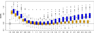
(b) $50\times 50$ grid with $m=23$

(c) $50\times 50$ grid with $m=77$

(d) $50\times 50$ grid with $m=77$

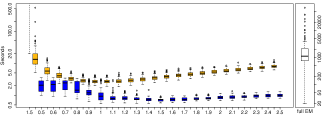
(e) $50\times 50$ grid with $m=175$

(f) $50\times 50$ grid with $m=175$

(g) $200\times 200$ grid with $m=23$

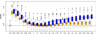
(h) $200\times 200$ grid with $m=23$

(i) $200\times 200$ grid with $m=77$

(j) $200\times 200$ grid with $m=77$

(k) $200\times 200$ grid with $m=175$

(l) $200\times 200$ grid with $m=175$

Figure S-5: Seconds (left panel) and Mean Squared Prediction Errors (MSPEs, right panel) for varying bandwidths constants (x-axis) and number of knots ($m$) for all three estimation methods on both grids when $\nu=1$ and $\sigma^{2}=0$.

(a) $50\times 50$ grid with $m=23$

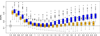
(b) $50\times 50$ grid with $m=23$

(c) $50\times 50$ grid with $m=77$

(d) $50\times 50$ grid with $m=77$

(e) $50\times 50$ grid with $m=175$

(f) $50\times 50$ grid with $m=175$

(g) $200\times 200$ grid with $m=23$

(h) $200\times 200$ grid with $m=23$

(i) $200\times 200$ grid with $m=77$

(j) $200\times 200$ grid with $m=77$

(k) $200\times 200$ grid with $m=175$

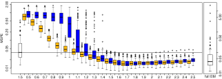
(l) $200\times 200$ grid with $m=175$

Figure S-6: Seconds (left panel) and Mean Squared Prediction Errors (MSPEs, right panel) for varying bandwidths constants (x-axis) and number of knots ($m$) for all three estimation methods on both grids when $\nu=1$ and $\sigma^{2}=0.1$.

(a) $50\times 50$ grid with $m=23$

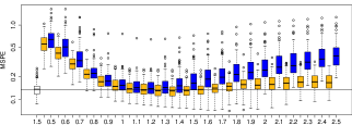
(b) $50\times 50$ grid with $m=23$

(c) $50\times 50$ grid with $m=77$

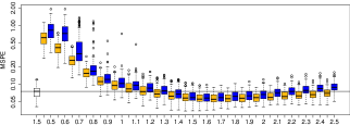
(d) $50\times 50$ grid with $m=77$

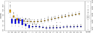
(e) $50\times 50$ grid with $m=175$

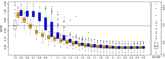
(f) $50\times 50$ grid with $m=175$

(g) $200\times 200$ grid with $m=23$

(h) $200\times 200$ grid with $m=23$

(i) $200\times 200$ grid with $m=77$

(j) $200\times 200$ grid with $m=77$

(k) $200\times 200$ grid with $m=175$

(l) $200\times 200$ grid with $m=175$

Figure S-7: Seconds (left panel) and Mean Squared Prediction Errors (MSPEs, right panel) for varying bandwidths constants (x-axis) and number of knots ($m$) for all three estimation methods on both grids when $\nu=1$ and $\sigma^{2}=0.25$.

(a) $50\times 50$ grid with $m=23$

(b) $50\times 50$ grid with $m=23$

(c) $50\times 50$ grid with $m=77$

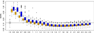
(d) $50\times 50$ grid with $m=77$

(e) $50\times 50$ grid with $m=175$

(f) $50\times 50$ grid with $m=175$

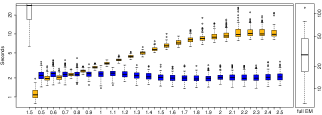
(g) $200\times 200$ grid with $m=23$

(h) $200\times 200$ grid with $m=23$

(i) $200\times 200$ grid with $m=77$

(j) $200\times 200$ grid with $m=77$

(k) $200\times 200$ grid with $m=175$

(l) $200\times 200$ grid with $m=175$

Figure S-8: Seconds (left panel) and Mean Squared Prediction Errors (MSPEs, right panel) for varying bandwidths constants (x-axis) and number of knots ($m$) for all three estimation methods on both grids when $\nu=1$ and $\sigma^{2}=0.4$.

(a) $50\times 50$ grid with $m=23$

(b) $50\times 50$ grid with $m=23$

(c) $50\times 50$ grid with $m=77$

(d) $50\times 50$ grid with $m=77$

(e) $50\times 50$ grid with $m=175$

(f) $50\times 50$ grid with $m=175$

(g) $200\times 200$ grid with $m=23$

(h) $200\times 200$ grid with $m=23$

(i) $200\times 200$ grid with $m=77$

(j) $200\times 200$ grid with $m=77$

(k) $200\times 200$ grid with $m=175$

(l) $200\times 200$ grid with $m=175$

Figure S-9: Seconds (left panel) and Mean Squared Prediction Errors (MSPEs, right panel) for varying bandwidths constants (x-axis) and number of knots ($m$) for all three estimation methods on both grids when $\nu=1.5$ and $\sigma^{2}=0$.

(a) $50\times 50$ grid with $m=23$

(b) $50\times 50$ grid with $m=23$

(c) $50\times 50$ grid with $m=77$

(d) $50\times 50$ grid with $m=77$

(e) $50\times 50$ grid with $m=175$

(f) $50\times 50$ grid with $m=175$

(g) $200\times 200$ grid with $m=23$

(h) $200\times 200$ grid with $m=23$

(i) $200\times 200$ grid with $m=77$

(j) $200\times 200$ grid with $m=77$

(k) $200\times 200$ grid with $m=175$

(l) $200\times 200$ grid with $m=175$

Figure S-10: Seconds (left panel) and Mean Squared Prediction Errors (MSPEs, right panel) for varying bandwidths constants (x-axis) and number of knots ($m$) for all three estimation methods on both grids when $\nu=1.5$ and $\sigma^{2}=0.1$.

(a) $50\times 50$ grid with $m=23$

(b) $50\times 50$ grid with $m=23$

(c) $50\times 50$ grid with $m=77$

(d) $50\times 50$ grid with $m=77$

(e) $50\times 50$ grid with $m=175$

(f) $50\times 50$ grid with $m=175$

(g) $200\times 200$ grid with $m=23$

(h) $200\times 200$ grid with $m=23$

(i) $200\times 200$ grid with $m=77$

(j) $200\times 200$ grid with $m=77$

(k) $200\times 200$ grid with $m=175$

(l) $200\times 200$ grid with $m=175$

Figure S-11: Seconds (left panel) and Mean Squared Prediction Errors (MSPEs, right panel) for varying bandwidths constants (x-axis) and number of knots ($m$) for all three estimation methods on both grids when $\nu=1.5$ and $\sigma^{2}=0.25$.

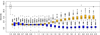
(a) $50\times 50$ grid with $m=23$

(b) $50\times 50$ grid with $m=23$

(c) $50\times 50$ grid with $m=77$

(d) $50\times 50$ grid with $m=77$

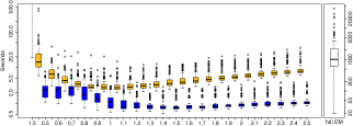
(e) $50\times 50$ grid with $m=175$

(f) $50\times 50$ grid with $m=175$

(g) $200\times 200$ grid with $m=23$

(h) $200\times 200$ grid with $m=23$

(i) $200\times 200$ grid with $m=77$

(j) $200\times 200$ grid with $m=77$

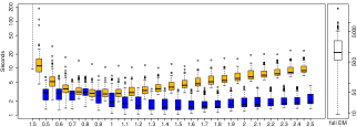
(k) $200\times 200$ grid with $m=175$

(l) $200\times 200$ grid with $m=175$

Figure S-12: Seconds (left panel) and Mean Squared Prediction Errors (MSPEs, right panel) for varying bandwidths constants (x-axis) and number of knots ($m$) for all three estimation methods on both grids when $\nu=1.5$ and $\sigma^{2}=0.4$.

(a) $50\times 50$ grid with $m=23$

(b) $50\times 50$ grid with $m=23$

(c) $50\times 50$ grid with $m=77$

(d) $50\times 50$ grid with $m=77$

(e) $50\times 50$ grid with $m=175$

(f) $50\times 50$ grid with $m=175$

(g) $200\times 200$ grid with $m=23$

(h) $200\times 200$ grid with $m=23$

(i) $200\times 200$ grid with $m=77$

(j) $200\times 200$ grid with $m=77$

(k) $200\times 200$ grid with $m=175$

(l) $200\times 200$ grid with $m=175$

Figure S-13: Seconds (left panel) and Mean Squared Prediction Errors (MSPEs, right panel) for varying bandwidths constants (x-axis) and number of knots ($m$) for all three estimation methods on both grids when $\nu=2$ and $\sigma^{2}=0$.

(a) $50\times 50$ grid with $m=23$

(b) $50\times 50$ grid with $m=23$

(c) $50\times 50$ grid with $m=77$

(d) $50\times 50$ grid with $m=77$

(e) $50\times 50$ grid with $m=175$

(f) $50\times 50$ grid with $m=175$

(g) $200\times 200$ grid with $m=23$

(h) $200\times 200$ grid with $m=23$

(i) $200\times 200$ grid with $m=77$

(j) $200\times 200$ grid with $m=77$

(k) $200\times 200$ grid with $m=175$

(l) $200\times 200$ grid with $m=175$

Figure S-14: Seconds (left panel) and Mean Squared Prediction Errors (MSPEs, right panel) for varying bandwidths constants (x-axis) and number of knots ($m$) for all three estimation methods on both grids when $\nu=2$ and $\sigma^{2}=0.1$.

(a) $50\times 50$ grid with $m=23$

(b) $50\times 50$ grid with $m=23$

(c) $50\times 50$ grid with $m=77$

(d) $50\times 50$ grid with $m=77$

(e) $50\times 50$ grid with $m=175$

(f) $50\times 50$ grid with $m=175$

(g) $200\times 200$ grid with $m=23$

(h) $200\times 200$ grid with $m=23$

(i) $200\times 200$ grid with $m=77$

(j) $200\times 200$ grid with $m=77$

(k) $200\times 200$ grid with $m=175$

(l) $200\times 200$ grid with $m=175$

Figure S-15: Seconds (left panel) and Mean Squared Prediction Errors (MSPEs, right panel) for varying bandwidths constants (x-axis) and number of knots ($m$) for all three estimation methods on both grids when $\nu=2$ and $\sigma^{2}=0.25$.

(a) $50\times 50$ grid with $m=23$

(b) $50\times 50$ grid with $m=23$

(c) $50\times 50$ grid with $m=77$

(d) $50\times 50$ grid with $m=77$

(e) $50\times 50$ grid with $m=175$

(f) $50\times 50$ grid with $m=175$

(g) $200\times 200$ grid with $m=23$

(h) $200\times 200$ grid with $m=23$

(i) $200\times 200$ grid with $m=77$

(j) $200\times 200$ grid with $m=77$

(k) $200\times 200$ grid with $m=175$

(l) $200\times 200$ grid with $m=175$

Figure S-16: Seconds (left panel) and Mean Squared Prediction Errors (MSPEs, right panel) for varying bandwidths constants (x-axis) and number of knots ($m$) for all three estimation methods on both grids when $\nu=2$ and $\sigma^{2}=0.4$.

References

• Bates and Maechler, (2015) Bates, D. and Maechler, M. (2015). Matrix: Sparse and Dense Matrix Classes and Methods. R package version 1.2-3.
• Davis, (2006) Davis, T. (2006). Direct Methods for Sparse Linear Systems. Fundamentals of Algorithms. Society for Industrial and Applied Mathematics.
• Nychka et al., (2015) Nychka, D., Furrer, R., Paige, J., and Sain, S. (2015). fields: Tools for Spatial Data. R package version 8.3-5.