Heterogeneous Doppler Spread-based CSI Estimation Planning for TDD Massive MIMO

Abstract

Massive multi-input multi-output (Massive MIMO) has been recognized as a key technology to meet the demand for higher data capacity and massive connectivity. Nevertheless, the number of active users is restricted due to training overhead and the limited coherence time. Current wireless systems assume the same coherence slot duration for all users, regardless of their heterogeneous Doppler spreads. In this paper, we exploit this neglected degree of freedom in addressing the training overhead bottleneck. We propose a new uplink training scheme where the periodicity of pilot transmission differs among users based on their actual channel coherence times. Since the changes in the wireless channel are, primarily, due to movement, uplink training decisions are optimized, over long time periods, while considering the evolution of the users channels and locations. Owing to the different rates of the wireless channel and location evolution, a two time scale control problem is formulated. In the fast time scale, an optimal training policy is derived by choosing which users are requested to send their pilots. In the slow time scale, location estimation decisions are optimized. Simulation results show that the derived training policies provide a considerable improvement of the cumulative average spectral efficiency even with partial location knowledge.

I Introduction

Future wireless networks have to address an exponentially increasing demand for high data-rate. In this context, several technologies have been proposed to improve the overall wireless networks performance: dense small-cell deployment, millimeter-wave communications and massive MIMO among others [1]. Massive MIMO was identified as one of the most promising technologies to meet this requirement. Originally introduced by Marzetta [2], massive MIMO exploits a large number of base station (BS) antennas in order to enable the spatial multiplexing of a large number of devices. By coherent processing of the signals over the BS antennas, transmit precoding can be used in order to concentrate each signal at its intended terminal and receive combining can be used in order to discriminate between the signals of different users. Massive MIMO have been thoroughly studied and have shown to improve the networks spectral efficiency (SE) and energy efficiency (EE) in addition to providing a high capacity per area [3]. These gains are conditioned by an accurate channel state information (CSI) at the BSs. In this paper we will focus on Time Division Duplexing (TDD) systems, where CSI can be acquired using uplink training with orthogonal pilot sequences [4]. A major issue in TDD systems is that a number of these pilot sequences are reused resulting in pilot contamination [2, 4, 5]. Another reason for CSI inaccuracy is channel aging. This phenomenon results from the variation of the channel between the instant when it is learned and the instant when it is used for signal processing. This time variation is due to users mobility and processing delays at the BS.

Performance degradation due to channel aging was studied in a MIMO system with coordinated multi-point transmission/reception (CoMP) in [6]. The authors showed that the impact of channel aging is mitigated when utilizing channel prediction filters in the low mobility regime. The authors in Truong et al. [7] provide an analysis of rate performance in the presence of channel aging and prediction. They showed that, although channel aging leads to degradation in the performance of massive MIMO systems, channel prediction can overcome this issue. In Papazafeiropoulos et al. [8, 9], the effect of channel aging combined with channel prediction has been investigated in scenarios with regularized Zero Forcing (ZF) precoders and minimum-mean-square-error (MMSE) receivers, respectively. In Kong et al. [10], lower bounds of the sum-rate for both Maximum Ratio Combining (MRC) and ZF receivers with/without channel prediction have been derived with an arbitrary number of BS antennas and users. The impact of channel aging and prediction on the power scaling law has been studied. The authors demonstrated that the transmit power scaling is not affected neither by aged CSI nor channel prediction.

Channel aging can also be leveraged in order to optimize uplink training. In Vu et al. [11], two spectral-efficient multiuser models for massive MIMO systems have been proposed. The main idea comes from the observation that users with low velocity are not required to send training sequences with the same periodicity as faster moving users owing to the resulting heterogeneous coherence times. The two proposed models proved to achieve significant SE gains.

In this paper, we aim at increasing the SE by exploiting the heterogeneous channel aging among users. In the current literature, the number of scheduled users, is limited by the fixed length of the uplink training reference signal. A more appropriate approach would be to define the needed training resources dynamically, at each time slot. We aim at adapting uplink training based on the actual coherence times. This means that, at a given slot, if the correlation between the estimated CSI and the actual channel was not considerably degraded, due to aging, the network is not required to reestimate it. Doing so enables to spear part of the training resources that can be used for data transmission or to schedule more users. This is in accordance with the concept of dynamic TDD that is already considered in the development of the 5G standard [21].

Channel aging results, primarily, from mobility, with speed being an important parameter. Consequently, developing an uplink training policy that takes into consideration the second order channel statistics is of paramount importance. Developing such policy requires accurate estimates of user locations, which can be rather complicated to obtain, in practice. In fact, localizing all scheduled users requires non negligible signaling, if it is done through the localization capabilities of the network (OTDOA [13] for example). Global Positioning System (GPS) can also be used but it rises the problem of the life span of mobile devices batteries [18]. Consequently, we suppose that the network is able to estimate the location of a limited set of users. Adapting to the change in the large-scale fading coefficients and optimizing uplink training decisions based on the channel’s autocorrelation should occur on two different time scales [14]. In fact the two optimizations are based on information that change over heterogeneous time scales. In order to achieve the maximum cumulative average SE over time spans larger than the large-scale fading coherence block, a two time scale control problem is considered.

In the fast time scale, an optimal training policy is derived. By taking into consideration the evolution over time of the correlation between the estimated CSI and the actual channel, the network is able to optimize its decisions to schedule users for uplink training over a finite time horizon. Taking into consideration the time dimension allows the network to be more efficient since it becomes able to predict the impact of its decisions on long term performance. Deriving such policy can naturally be formulated as a discrete planning problem over a finite time horizon [15]. The optimal training decisions are derived for a predefined time duration, denoted here by $H$, for which the large-scale fading coefficients are supposed to be constant. This is quite advantageous since it allows to optimize training over time without requiring the actual channel estimates. Results prove that the derived training policy provides substantial performance increase. Since deriving the optimal policy can be computationally prohibitive for large optimization horizons, we provide a combinatorial optimization framework that enables to derive an approximate training policy with reduced running time.

In the slow time scale, the network adapts to user mobility by deciding which users are required to feedback their locations. Estimating the exact location of all users requires a non negligible signaling overhead. Consequently, efficiently selecting the users that are required to feedback their location is important. Since locations are estimated in a periodic manner, we consider user locations that evolve according to independent Markovian stochastic processes [20]. The location estimation problem introduced above, with locations evolving in a Markovian fashion, can be formulated as a Partially Observable Markov Decision Process (POMDP)[19]. Simulations prove that the combined optimization, on the two time scales, provides an efficient training strategy that improves the achievable cumulative average SE even with partially erroneous geolocalisation.

This paper is organized as follows. We describe the considered system model in Section II. We discuss the advantages of coherence time based training in Section III. Two time scale training strategy learning is discussed in Section IV. Finally, in Section V, numerical results are presented.

II System Model And Preliminaries

We consider the uplink of a multi-cell multiuser massive MIMO system constituted of $C$ macro BSs operating in TDD mode. Each macro BS is equipped with $M$ omnidirectional antennas and serves $K$ mobile devices equipped, each, with a single omnidirectional antenna. We will refer to the latter as users. All users in the network move according to different speeds and directions. Consequently, their signals are subject to heterogeneous Doppler spreads which results in different wireless channel autocorrelations in time. We consider a system where time is slotted $t\in\{0,1,\ldots\}$ and the duration of each time slot $t$ is given by $D_{c}$. We note that $D_{c}$ is the channel coherence time which depends on the maximum Doppler spread supported by the network, see for instance Toufik et al. [13]. We also consider the corresponding coherence interval $T_{s}$. The wireless channel of each user can be decomposed as a product of small and large scale fading coefficients. The wireless channel from user $k$ (in cell $c$) to BS $j$, at time slot $t$, i.e., $g^{[j]}_{kc}(t)$, is given by

$$g^{[j]}_{kc}(t)=\sqrt{\beta^{[j]}_{kc}}h^{[j]}_{kc}(t),\text{ for all }k=1,\ldots,K,\text{ and }j,c=1,\ldots,C,$$ (1)

where $h^{[j]}_{kc}(t)\in\mathbb{C}^{M\times 1}$ is the fast fading vector, $h^{[j]}_{kc}(t)\sim\mathcal{C}\mathcal{N}(0,I_{M})$. ${\beta^{[j]}_{kc}}\in\mathbb{R}^{+}$ models the large-scale effect including shadowing and pathloss, which are assumed to remain constant during large-scale coherence blocks of $T_{\beta}$ OFDM symbols.

Remark 1.

In Sections IV and V we will consider a system where $\beta^{[j]}_{kc}$ evolves according to a Markovian model.

II-A Channel Estimation

As introduced above, in this paper we focus on a TDD system, where the entire frequency band is used for downlink and uplink transmission by all BSs and users. The BSs acquire CSI estimates using orthonormal training sequences (i.e., pilot sequences) in the uplink. We consider a pilot reuse factor of $1$, i.e. the same sets of pilot sequences are used in all cells.

We also consider that, during each coherence interval, a maximum of $\tau$ users are scheduled for uplink training in each cell with $\tau\leq K$. For that, we consider a set of orthonormal training sequences, that is, sequences $q_{i}\in\mathbb{C}^{\tau\times 1}$ such that $q^{\dagger}_{i}q_{j}=\delta_{ij}$ (with $\delta_{ij}$ the Kronecker delta).

During uplink training of slot $t$, the $l^{th}$ BS receives the pilot signal $Y^{[l]}_{p}(t)\in\mathbb{C}^{M\times\tau}$

$$Y^{[l]}_{p}(t) =\sum_{c=1}^{C}\sum_{k=1}^{\tau}\sqrt{P_{p}}g^{[l]}_{kc}(t)q^{\dagger}_{k}+W_{p}(t),$$ (2)

where $W_{p}(t)\in\mathbb{C}^{M\times\tau}$ refers to an additive white Gaussian noise matrix with i.i.d. $\mathcal{C}\mathcal{N}(0,1)$ entries. $P_{p}$ refers to the training signal power. The $l^{th}$ BS then uses the orthogonality of training sequences in order to obtain the MMSE estimate of the channel of user $k,l$ [5] as

$$\hat{g}_{kl}^{[l]}(t)=\frac{\beta^{[l]}_{kl}}{\frac{1}{P_{p}}+\sum_{b,b\neq l}^{C}\beta^{[l]}_{kb}}\frac{Y^{[l]}_{p}(t)}{\sqrt{P_{p}}}q_{k}.$$ (3)

Note that the MMSE channel estimate $\hat{g}^{[l]}_{kl}(t)$ follows a $\mathcal{C}\mathcal{N}\left(0,\frac{\beta^{[l]^{2}}_{kl}}{\frac{1}{P_{p}}+\sum_{b,b\neq l}^{C}\beta^{[l]}_{kb}}I_{M}\right)$ distribution. The wireless channel between user $k$ (in cell $l$) and BS $l$ can then be decomposed as follows

$$g_{kl}^{[l]}(t)=\hat{g}_{kl}^{[l]}(t)+\tilde{g}_{kl}^{[l]}(t),$$ (4)

where $\tilde{g}_{kl}^{[l]}(t)$ represents the estimation error and follows a $\mathcal{C}\mathcal{N}\left(0,\left(\beta^{[l]}_{kl}-\frac{\beta^{[l]^{2}}_{kl}}{\frac{1}{P_{p}}+\sum_{b,b\neq l}^{C}\beta^{[l]}_{kb}}\right)I_{M}\right)$ distribution. Moreover, $\hat{g}^{[l]}_{kl}(t)$ and $\tilde{g}^{[l]}_{kl}(t)$ are independent [5].

II-B Channel aging

In practice, the wireless channel varies between the time when it is learned and used for precoding in downlink and decoding in uplink. This variation is due mainly to user movement and processing delays. Such phenomenon is referred to as channel aging. Its impact can be captured by a time varying wireless channel model. To this end we consider a stationary ergodic Gauss-Markov block fading regular process (or auto-regressive model of order 1) [16]. The evolution of the channel vector of user $k,l$ between the two slots $t$ and $t-1$ is expressed as

$$g^{[l]}_{kl}(t)=\rho_{kl}^{[l]}{g}^{[l]}_{kl}(t-1)+\sqrt{\beta^{[l]}_{kl}}\varepsilon^{[l]}_{kl}(t),$$ (5)

where $\varepsilon^{[l]}_{kl}(t)$ denotes a temporally uncorrelated complex white Gaussian noise process with zero mean and variance $(1-\rho^{[l]^{2}}_{kl})I_{M}$. $\rho^{[l]}_{kl}$ represents a temporal correlation parameter of the channel of user $k,l$. This parameter is given by Jakes et al. [16] and reads as follows

$$\rho^{[j]}_{kl}=J_{0}(2\pi f^{[j]}_{kl}D_{c}),$$ (6)

where $J_{0}(\cdot)$ is the zeroth-order Bessel function of the first kind and $f^{[j]}_{kl}$ represents the maximum Doppler shift of user $k$ in cell $l$ with respect to the antennas of BS $j$. In our work, we adopt a realistic setting in which, mobile users have different frequency shifts since we consider heterogeneous movement velocities and directions. For every user $k$ in cell $l$, the maximum Doppler shift with respect to the antennas of BS $j$ is given by

$$f^{[j]}_{kl}=\frac{\nu_{kl}f_{\textit{c}}}{\textit{c}}\text{cos}(\theta^{[j]}_{kl}),$$ (7)

where $\nu_{kl}$ is the velocity of user $k$ in cell $l$ in meters per seconds, $\textit{c}=3\times 10^{8}\;\text{mps}$ is the speed of light, $f_{\textit{c}}$ is the carrier frequency and $\theta^{[j]}_{kl}$ represents the angular difference between the directions of the mobile device movement and the incident wave. Taking into consideration the combined effects of estimation error and impairments due to channel aging, we can express the wireless channel of user $k,l$ at time $t$ as

$$g^{[l]}_{kl}(t)=\rho_{kl}^{[l]}\hat{g}^{[l]}_{kl}(t-1)+\rho_{kl}^{[l]}\tilde{g}^{[l]}_{kl}(t-1)+\sqrt{\beta^{[l]}_{kl}}\varepsilon^{[l]}_{kl}(t),$$ (8)

III An adaptive uplink training approach for Massive MIMO TDD systems

In current Massive MIMO models, the same coherence interval $T_{s}$ is considered for all users. $T_{s}$ is defined as a system parameter that is based on the maximum Doppler spread supported by the network [13]. This consideration results in a suboptimal use of the time-frequency resources and a loss of flexibility that can be leveraged otherwise. In fact, in practice, users experience heterogeneous Doppler spreads. Consequently, their channels do not age at the same rate. Forcing all users to perform uplink training with the same periodicity causes vain redundancy and a loss of resources. A more efficient approach should adapt the periodicity of each user CSI estimation according to its actual coherence time [12] [11]. This means that, at a given slot, if the correlation between the estimated CSI and the actual channel was not considerably degraded, the network is not required to reestimate it. Doing so enables to spear part of the training resources that can be used for data transmission or to schedule more users. In all cases, the latter results in an increase in SE. In this section, we present a novel approach for uplink training that leverages the users heterogeneous channel coherence times. We present a detailed analysis of its impact on the achievable SE with MRC receivers. We also derive an important condition which ensures that the proposed scheme is able to improve performance.

III-A An adaptive coherence time-based uplink training scheme

We consider a massive MIMO system in which CSI estimation is adapted according to the actual users’ coherence times. We consider that the network groups users according to their channel autocorrelation coefficients into $N_{G}$ copilot user groups $\lambda_{g},\;g=1,...,N_{G}$. The users in each group are either scheduled for uplink training synchronously, using the same pilot sequence, or not scheduled at all. This requirement guarantees that copilot users always have the same CSI delay and a similar channel aging effect. For each copilot group $\lambda_{g},\;g=1,...,N_{G}$, the CSI delays are denoted by $d_{g},g=1,...,N_{G}$. At each slot, all $N_{G}$ copilot user groups are scheduled for data transmission and a maximum of $\tau\;(\tau<N_{G})$ copilot groups are selected for uplink training. The rest will have their signals processed using the last estimated version of their CSI. The proposed Time-Division Duplexing (TDD) protocol consists of the following seven steps.

1. In the beginning of each large-scale coherence block, the BSs estimate the large scale fading and channel autocorrelation coefficients, i.e., $\beta_{kc}^{[j]}$ and $\rho_{kc}^{[j]}$ for all $k=1,\ldots,K$, and $c,j=1,\ldots,C$. All coefficients are then fed back to a central processing unit (CPU).

2. Next, the CP clusters users according to their autocorrelation coefficients using $K$-mean, see Young et al [17]. The resulting clusters will be characterized by an average autocorrelation coefficient or, equivalently, an average Doppler spread and a variance of the corresponding users autocorrelation coefficients. The considered number of clusters is $N_{c}$. Defining $N_{c}$ is of paramount importance. In this work, we choose to define $N_{c}$ according to

   $$N_{c}=\lceil\frac{D_{max}}{D_{c}}\rceil,$$ (9)

   where $D_{max}$ represents the maximum coherence time. $(9)$ guarantees that the average coherence time per cluster is approximately equivalent to a multiple of $D_{c}$. This is needed in order to appropriately define CSI estimation periodicity as a function of the parameter $D_{c}$.

3. Next, the CP allocates all users in the network ($K$ per cell) to $N_{G}$ copilot groups. Each group contains at maximum $C$ users from the same channel autocorrelation based cluster and from different cells. These $N_{G}$ copilot groups are formed with minimum variance of the autocorrelation coefficients in each group. This guarantees that copilot users has similar channel aging impact. The justification for this grouping is discussed in Section III.C.

4. At each coherence slot, the network schedules at maximum $\tau$ copilot groups for uplink training synchronously. Depending on the main key performance indicator (KPI) to optimize, different scheduling algorithms can be used to select these copilot groups. In this paper, we propose a scheduling algorithm that exploits the aforementioned user grouping in order to derive an optimal CSI estimation policy. This is the focus of Section IV and represents one of the main contributions of the present work.

5. All $N_{G}$ copilot groups transmit their uplink signal in a synchronous manner.

6. The BSs process the received pilot signal and estimates the channels of the active users during uplink training using MMSE estimators. The BSs decode and precode the uplink and downlink data signals, respectively, using the last estimated version of each user CSI.

7. All BSs synchronously transmit downlink data signals to the $N_{G}$ copilot groups.

III-B Spectral efficiency with outdated CSI

In what follows, we analyze the impact of the aforementioned training procedure on the achievable SE with a MRC receiver. We also explain why an adaptive Doppler based training can be more efficient. Moreover, we provide a condition in order to ensure that the spectral efficiency of all users is improved when the aforementioned training procedure is used. For the sake of analytical traceability, we consider that the $N_{G}$ copilot groups contain exactly $C$ users. We, henceforth, refer to each user by its copilot group and serving BS indexes. During uplink data transmission, at time slot $t$, BS $l$ receives the data signal $Y^{[l]}_{u}(t)$ which is given by

$$Y^{[l]}_{u}(t)=\sum_{c=1}^{C}\sum_{k=1}^{N_{G}}\sqrt{P_{u}}g^{[l]}_{kc}(t)S_{kc}+W_{u}(t),$$ (10)

where $W_{u}(t)\sim CN(0,I_{M})$ is the additive noise, $S_{kc}$ denotes the uplink signal of user $k,c,\;k=1,\ldots,N_{G},\;c=1,\ldots,C$ and $P_{u}$ denotes the reverse link transmit power. Each BS applies a MRC receiver based on the latest available CSI estimates. BS $l,l=1,\ldots,C$ detects the signal of user $g,g=1,\ldots,N_{G}$, within the same cell, by applying the following

$$u_{gl}(t)=\frac{\hat{g}^{[l]}_{gl}(t-d_{g})}{\lVert\hat{g}^{[l]}_{gl}(t-d_{g})\rVert},t\geq d_{g},$$ (11)

where $\hat{g}^{[l]}_{gl}(t-d_{g})$ denotes the latest available channel estimate of user $g$ in cell $l$. The resulting average achievable SE in the system with MRC receivers is given in Theorem $1$.

Theorem 1.

For $N_{G}$ active copilot groups, $\tau$ of which are scheduled for uplink training and using a MRC receiver $u_{gl}(t)$ that is based on the latest available CSI estimates of each user $g,l$, the average achievable spectral efficiency in the uplink $\bar{R}^{MRC}_{u}$ is lower bounded by:

$$\bar{R}^{MRC}_{u}\geq\sum_{l=1}^{C}\sum_{g=1}^{N_{G}}\left(1-\frac{\tau}{T_{s}}\right)\text{log}\left(1+\frac{(M-1)\beta^{[l]^{2}}_{gl}\rho^{[l]^{2d_{g}}}_{gl}}{(M-1)\times I^{p}_{gl}+I^{n}_{gl}}\right),$$ (12)

where $d_{g},g=1...N_{G}$ represents the copilot groups CSI delays. $I^{p}_{gl}$ and $I^{n}_{gl}$ are given by:

$$I^{p}_{gl}=\sum_{c\neq l}^{C}\rho^{[l]^{2d_{g}}}_{gc}\beta^{[l]^{2}}_{gc},$$ (13)

$$I^{n}_{gl}=(\sum_{c=1}^{C}\sum_{k\neq g}^{N_{G}}\beta^{[l]}_{kc}+\sum_{c=1}^{C}(\beta^{[l]}_{gc}-\rho^{[l]^{2d_{g}}}_{gc}\frac{\beta^{[l]^{2}}_{gc}}{\frac{1}{P_{p}}+\sum_{b=1}^{C}\beta^{[l]}_{gb}})+\frac{1}{P_{u}})\times(\frac{1}{P_{p}}+\sum_{b=1}^{C}\beta^{[l]}_{gb}).$$

Proof:

See appendix A. ∎

Equation (12) provides further insights into the impact of channel aging on the achievable average SE as a function of the CSI time offset. We can clearly see that the SE decreases as a function of its CSI time offset. This is an intuitive result since the correlation between the estimated CSI and the actual channel fades over time. Equation (12) shows also that for a same CSI time offset, the degradation due to channel aging is higher for users with lower autocorrelation coefficients. Although outdated CSI causes an SINR degradation, the speared resources from uplink training can lead to an increase in SE.

III-C ASYMPTOTIC Performance

We now analyze the potential gain that the proposed training approach can provide. To do so, we compare it with a reference model that follows a classical TDD protocol in which all of $N_{G}$ copilot groups are scheduled for uplink training at each time slot. We consider a worst case scenario with random delays and random copilot groups allocation. In this scenario, each user experiences the lowest channel autocorrelation coefficient in comparison with its copilot users. This means that each user suffers from the heaviest channel aging impact in its copilot group.

Theorem 2.

In the asymptotic regime ($M$ grows large), with $\bar{\rho}^{[{min}]}_{g}$ and $\bar{\rho}^{[{max}]}_{{g}}$ denoting, respectively, the minimum and maximum autocorrelation coefficients in copilot group $g,\;g=1,...,N_{G}$, the proposed training framework enables to improve the SE of each user when (14) is satisfied

$$\left(\frac{\bar{\rho}^{[{min}]^{2}}_{g}}{\bar{\rho}^{[{max}]^{2}}_{{g}}}\right)^{d_{g}}\geq\frac{\left(1+\text{ SINR}^{[\infty]}_{g,l}\right)^{\frac{T_{s}-N_{G}}{T_{s}-\tau}}-1}{\text{ SINR}^{[\infty]}_{g,l}},$$ (14)

with

$$\text{ SINR}^{[\infty]}_{g,l}=\frac{\beta^{[l]^{2}}_{gl}}{\sum_{c\neq l}\beta^{[l]^{2}}_{gc}},$$ (15)

Proof:

See appendix B. ∎

Condition (14) ensures that the SE of each user increases when outdated CSI is used. Equation (14) shows that the speared resources due to the reduced training overhead is a defining parameter. In fact, SE is improved as long as the SINR degradation is compensated for by the spared resources from training. It also shows the importance of the ratio between the minimum and maximum autocorrelation coefficients in a copilot group. A high ratio is required in order to achieve the needed SE gain. This requirement become tighter as the CSI time offset increases. (14) shows that the use of the proposed procedure can improves the achievable SE even with random delays and random pilot sequence allocation.

Remark 2.

In order to satisfy condition (14), copilot users need to have similar autocorrelation coefficients. This explains Steps $2)$ and $3)$ in the protocol in Section III.A. In fact, clustering users based on their autocorrelation coefficients and grouping them accordingly results in copilot user groups with homogeneous channel aging within each group. This allows to tolerate higher CSI time offset. (14) also shows that the use of the aforementioned training procedure can improves the achievable SE of the network, even with random pilot allocation. Consequently, one can do better if a coherence time adaptive scheduling for uplink training is implemented. More importantly, the proposed scheme shows the impact of the time dimension. This fact justifies the need for a time-aware training optimization which will be the focus of the next section.

IV Optimal training strategy with outdated CSI and user mobility: a two-time scale decision process

We proved that adapting uplink training periodicity to the actual channel coherence time can provide a considerable increase in network performance, even with random pilot sequence allocation. Nevertheless, higher performance gain can be obtained if more sophisticated and adapted scheduling policy is used. Developing such policy is the focus of this section.

As a matter of fact, knowing that CSI estimation periodicity should depend on the rate of channel aging, it makes sense to develop an uplink training policy that takes into consideration the evolution in the difference between the estimated CSI and the actual wireless channels. In opposition to a per slot uplink training optimizing, such policy enables to take into consideration the impact of past scheduling decisions on the long term performance. User mobility should also be included. In fact, channel aging results, primarily, from mobility, with velocity being a defining parameter. Consequently, developing an uplink training policy that takes into consideration the evolution of large-scale fading coefficients, in addition to channel aging, is of paramount importance. Developing such strategy requires accurate estimates of user locations, which can be rather complicated to obtain, in practice. As a matter of fact, localizing all covered users requires a non negligible signaling overhead and energy consumption [13], [18]. Consequently, this problem should be addressed while assuming a partial knowledge of the user positions. Adapting to the change in user locations and optimizing uplink training decisions based on the channels’ autocorrelation coefficients, should occur on two different time scales [14]. In fact, the two optimizations are based on information that change over heterogeneous time scales (The wireless channel changes faster than user position). Consequently, a two time scale control problem should be formulated. This will be the focus of the present section.

IV-A Optimizing uplink training: A two-time scale control problem

We now model the two-time scale system introduced above as a POMDP [19]. We assume finite action and state spaces in both time scales (see Figure 1).

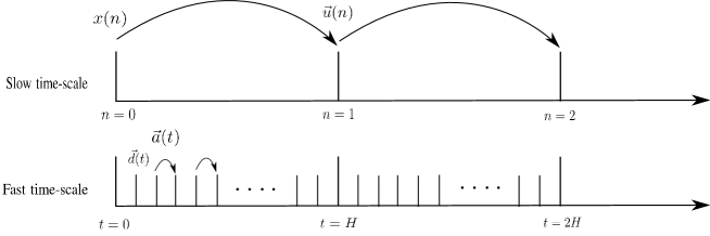
Figure 1: A two time-scale planning problem

We consider that, in the slow-time scale (upper level), the position of the users evolves according to a Markovian Mobility model [20] within its serving cell. These position variations occur at decision times $n=0,1,\ldots$. Let $\ell_{g}(n)$ be the combination of the positions of users from copilot group $g$ at time $n$. Considering the combination of copilot users positions instead of each individual one enables to reduce the complexity of the present model. We assume, for the sake of simplicity, that all copilot groups have $L$ possible position combinations, hence $\ell_{g}(n)\in\{1,\ldots,L\}$. Building this model requires a portioning of the coverage area of each cell into a number of disjoint regions. The area of each region is chosen such that the variation of the large scale fading coefficients can be considered as negligible within the region. For copilot group $g$, each position $\ell_{g}(n)\in\{1,\ldots,L\}$ corresponds to a combination of regions in each cell. The transition probabilities are characterized by the matrix

$$P_{g}=(p_{g}(i,j))_{i,j\in\{1,\ldots,L\}},\hbox{ for copilot group }g.$$ (16)

The large scale fading coefficients for user $g$ in cell $l$, i.e., $\beta_{gl}^{[j]},j\in\{1,\ldots,C\}$ depend on the users’ position. In previous sections, we assumed that this values were constant. In this section, we add a time dependency to it, namely, $\beta_{gl}^{[j]}(n)=\beta_{gl}^{[j],\ell_{g}(n)}\in\{\beta_{gl}^{[j],1},\ldots,\beta_{gl}^{[j],L}\}$. Acquiring the information on the position of all users can be really expensive in terms of processing overhead and energy consumption [13],[18]. Consequently, we consider that a limited number of users can feedback its positions to the network. In particular, we assume that, in every decision epoch, the users from $U_{max}$ copilot groups can feedback their positions (with $U_{max}<N_{G}$). The CP therefore can only acquire the positions of the users from $U_{max}$ copilot groups, at each time $n$. The positions of the rest of the user will be inferred from previous estimations. This estimation is characterized by the belief state vector. The belief state vector of copilot group $g$, at decision-time $n$, will be denoted by $\vec{b}_{g}(n)$, where the $i^{th}$ entry in $\vec{b}_{g}(n)$ refers to the probability that the users of copilot group $g$ are in positions of combination $i$. We define by $\mathcal{X}_{g}$ the set of all belief states for copilot group $g$ and we let $\mathcal{X}=\mathcal{X}_{1}\times\ldots\times\mathcal{X}_{N_{G}}$ be the state space in the upper level. A remark on the notation is now in order.

Remark 3.

The state in the upper level $x\in\mathcal{X}$ is an $L\times N_{G}$ matrix, whose columns represent the belief state vectors of all copilot groups $g$, for $g=1,\ldots,N_{G}$. That is, $x=(\vec{b}_{1},\ldots,\vec{b}_{N_{G}})$.

In the upper level, at every decision epoch $n=0,1,\ldots$, the decision is to select which $U_{max}$ copilot groups out of the $N_{G}$ will transmit their positions to the BSs. That is, we consider the action vector $\vec{u}(n)=(u_{1}(n),\ldots,u_{N_{G}}(n))\in\mathcal{A}=\{0,1\}^{N_{G}}$, such that

$$u_{g}(n)=\begin{cases}1&\mbox{ users in copilot group $g$ feedback their positions at decision epoch $n$,}\\ 0&\mbox{otherwise. }\end{cases}$$ (17)

At decision epoch $n$, the transition probability from belief state matrix $x(n)\in\mathcal{X}$ to belief state matrix $x(n+1)\in\mathcal{X}$ is defined by

$$\mathbb{P}^{up}(x(n+1)=x^{\prime}|x(n)=x,\vec{u}(n))= \mathbb{P}(\vec{b}_{1}(n+1)=b_{1}^{\prime}|\vec{b}_{1}(n)=b_{1},\vec{u}(n))\cdot\ldots$$ (18)

$$\cdot\mathbb{P}(\vec{b}_{N_{G}}(n+1)=b_{N_{G}}^{\prime}|\vec{b}_{N_{G}}(n)=b_{N_{G}},\vec{u}(n)),$$

where, $x^{\prime}=(\vec{b}_{1}^{\prime},\ldots,\vec{b}_{N_{G}}^{\prime})$, $x=(\vec{b}_{1},\ldots,\vec{b}_{N_{G}})$ with $b_{g}^{\prime},b_{g}\in\mathcal{X}_{g}$ for all $g=1,\ldots,N_{G}$ and $\vec{u}(n)\in\mathcal{A}$. The latter is satisfied because all users have independent movements. Recall that each position combination of users in copilot group $g$ is characterized by a set of large scale fading coefficients $\beta_{gl}^{[j]},j\in\{1,\ldots,C\},\;l\in\{1,\ldots,C\}$. In the fast-time scale, we define the state-space by $X=\{0,\ldots,H-1\}^{N_{G}}$, that is, the set of all possible delay vectors. Namely, $\vec{d}=(d_{1},\ldots,d_{N_{G}})\in X$ is such that $d_{g}$ is the CSI delay of all users in copilot group $g$, i.e., $\lambda_{g}$. The action space is $A=\{0,1\}^{N_{G}}$. For $\vec{a}=(a_{1},\ldots,a_{N_{G}})\in A$, $a_{g},1,\ldots,{N_{G}}$ is given by

$$a_{g}=\begin{cases}1&\mbox{ copilot group $g$ is scheduled for uplink training,}\\ 0&\mbox{otherwise. }\end{cases}$$ (19)

The decision times at the fast-time scale (lower level) will be denoted by $t=\{t_{0},t_{1},\ldots\}$, with $t_{nH}=n$ for all $n=0,1,\ldots$ and $H$ the finite-time horizon in the lower level. Moreover, we make the assumption that the decision $\vec{u}(n+1)$, in the slow-time scale, is made right after the decision at time $t_{nH}$. We denote by $\vec{d}(0)=\vec{d}^{0}\in X$ the initial state in the fast-time scale at $n=0$ and $x_{0}\in\mathcal{X}$ the initial state in the slow-time scale. In this particular model, the fast time scale transitions from time $t_{nH}$ until time $t_{(n+1)H-1}$ for all $n\geq 0$ are deterministic. Namely,

$$d_{g}(t_{nH+j})=(1+d_{g}(t_{nH+j-1}))(1-a_{g}(t_{nH+j})),\hbox{ for all }n\geq 0,\hbox{ and }1\leq j\leq H.$$ (20)

At the fast time scale, we therefore encounter a finite-state finite-horizon deterministic sequential-decision problem [15]. The reward in this level, at time $t$ with MRC receivers, is the following

$$R^{low}(\vec{d}(t),\vec{a}(t),x,\vec{u})=\sum_{g=1}^{N_{G}}\sum_{l=1}^{C}\left(1-\frac{1}{T_{s}}\sum_{i=1}^{N_{G}}a_{i}(t)\right)\log\left(1+\hbox{SINR}_{gl}^{MRC}(\vec{d}(t),x,\vec{u})\right),$$ (21)

where $x\in\mathcal{X}$ and $\vec{u}\in\mathcal{A}$ are fixed and

$$\hbox{SINR}_{gl}^{MRC}(\vec{d}(t),x,\vec{u})=\frac{(M-1)(\beta_{gl}^{[l]})^{2}(\rho_{gl}^{[l]})^{2d_{g}(t)}}{(M-1)\times I_{gl}^{p}+I_{gl}^{n}},$$ (22)

the SINR of user $g$ in cell $l$ with MRC receiver. $I^{p}_{gl}$ and $I_{gl}^{n}$ are given in Theorem $1$.
Note that the reward function at the lower level, i.e., $R^{low}$, depends on the belief state and the decision in the upper level. We now define the sequence $\pi^{low}=\{\vec{\phi}^{low}_{n}\}_{n=0}^{\infty}$, where for each $n$,

$$\vec{\phi}_{n}^{low}=(\phi_{t_{nH}}^{low},\phi^{low}_{t_{nH+1}},\ldots,\phi^{low}_{t_{(n+1)H-1}}).$$ (23)

Each function $\phi_{t_{nH+j}}^{low}:X\times\mathcal{X}\times\mathcal{A}\to A$ prescribes the action to be taken at decision time $t_{nH+j}$ (in the lower level), for all $n\geq 0$ and all $0\leq j\leq H-1$. For this model we only look at the set of stationary decision rules, $\pi^{low}$ with respect to the upper level, such that $\vec{\phi}_{n}^{low}(\vec{d},x,\vec{u})=\vec{\phi}_{n^{\prime}}^{low}(\vec{d},x,\vec{u})$ for all $n$ and $n^{\prime}$ given $\vec{d}\in X$, $x\in\mathcal{X}$ and $\vec{u}\in\mathcal{A}$. That is, for fixed $\vec{d}\in X$, $x\in\mathcal{X}$ and $\vec{u}\in\mathcal{A}$ the optimal decision rule in the lower level will be independent of the decision epoch $n$ in the slow time scale. This consideration is in accordance with most existing literature and can also be justified by the considered setting. The set of all possible lower level decision rules will be denoted by $\Pi^{low}$, i.e., $\pi^{low}\in\Pi^{low}$. Moreover, we drop the dependency on $n$, since we only consider policies that are $n$-independent, and we denote by $\Phi^{low}$ the set of all $H$-horizon policies $\vec{\phi}^{low}$, i.e., $\vec{\phi}^{low}\in\Phi^{low}$. We now define $\Phi^{low}_{x,\vec{u}}\subset\Phi^{low}$ as follows

$$\Phi^{low}_{x,\vec{u}}=\{ \vec{\phi}^{low}_{x,\vec{u}}:\vec{\phi}^{low}_{x,\vec{u}}=(\phi^{low}_{x,\vec{u},t_{0}},\ldots,\phi^{low}_{x,\vec{u},t_{H-1}}),\phi^{low}_{x,\vec{u},t_{j}}:X\times\{x\}\times\{\vec{u}\}\to A\hbox{ and }j=0,\ldots,H-1\}.$$ (24)

The latter is the set of all $H$-horizon policies given initial belief state matrix $x$ and action in the upper level $\vec{u}$. Note that, in the definition of $\Phi^{low}_{x,\vec{u}}$ to introduce the policy $\vec{\phi}^{low}_{x,\vec{u}}$, we use the decision times $t_{0},\ldots,t_{H-1}$. This is without loss of generality, since we recall that these policies are independent from $n$. Next we define the reward in the upper level. Namely,

$$R^{up}(\vec{d},\vec{\phi}^{low},x(n),\vec{u}(n))=\sum_{t=t_{nH}}^{t_{(n+1)H-1}}R^{low}(\vec{d}(t),\phi_{t}^{low}(\vec{d}(t),x(n),\vec{u}(n)),x(n),\vec{u}(n)),$$ (25)

where $\vec{d}$ is the delay state vector at time $t_{nH}$. We remark that none of the upper level decisions incur in an immediate cost. Let us denote by $\Phi^{up}$ the set of all possible stationary decision rules in the upper level, such that $\pi^{up}\in\Phi^{up}$, $\pi^{up}:X\times\mathcal{X}\to\mathcal{A}$. Consequently, the objective is to find $\pi^{up}\in\Phi^{up}$ and $\pi^{low}\in\Phi^{low}$ such that

$$\max_{\pi^{up}\in\Phi^{up}}\max_{\pi^{low}\in\Phi^{low}}\lim_{Z\to\infty}\frac{1}{Z}\sum_{n=0}^{Z-1}\mathbb{E}\left(R^{up}(\vec{d}(t_{nH}),\pi^{low},x(n),\pi^{up}(\vec{d}(t_{nH}),x(n)))\right).$$ (26)

The latter problem is a POMDP [19]. To see this, it suffices to note that the slow time scale sequential decision making problem is just a POMDP with a reward that depends on the fast time scale deterministic decision making problem. Therefore the standard theory on Bellman’s optimality equations follows. The optimal decision-rule for this POMDP can be obtained as a solution of the optimality equation for $0<\alpha<1$

$$V(\vec{d},x)=\max_{\vec{u}\in\mathcal{A}}\left(\max_{\vec{\phi}^{low}_{x,\vec{u}}\in\Phi^{low}}\{R^{up}(\vec{d},\vec{\phi}^{low}_{x,\vec{u}},x,\vec{u})+\alpha\sum_{y\in\mathcal{X}}\mathbb{P}^{up}(y|x,\vec{u})V(\vec{d}^{\vec{\phi}^{low}_{x,\vec{u}}},y)\}\right).$$ (27)

$V(\vec{d},x)$ denotes the value function [19] which refers, in our case, to the long term SE. We will now make an assumption that simplifies the model significantly. We define $\overline{\Phi}^{low}\subset\Phi^{low}$ where

$$\overline{\Phi}^{low}=\{ \vec{\phi}^{low}:\vec{\phi}^{low}=(\phi_{t_{0}}^{low},\ldots,\phi_{t_{H-1}^{low}}),$$ (28)

$$\phi^{low}_{t_{j}}:X\times\{x\}\times\{\vec{u}\}\to A\hbox{ for }j=0,\ldots,H-1,\hbox{ and }\phi^{low}_{t_{0}}=(1,\ldots,1)\}.$$

For all $\vec{\phi}^{low}\in\overline{\Phi}^{low}$, $\vec{\phi}^{low}$ is such that, in the first stage of the $H$-horizon problem, all copilot groups are scheduled for uplink training. This allows us to start every slow-time scale with the same delay state $\vec{d}(nH)=(0,\ldots,0)$ for all $n=0,1,\ldots$. Eq. (27) then reduces to

$$V(x)=\max_{\vec{u}\in\mathcal{A}}\left(\max_{\vec{\phi}^{low}_{x,\vec{u}}\in\overline{\Phi}^{low}}\{R^{up}(\vec{\phi}^{low}_{x,\vec{u}},x,\vec{u})\}+\alpha\sum_{y\in\mathcal{X}}\mathbb{P}^{up}(y|x,\vec{u})V(y)\right),$$ (29)

where $R^{up}(\vec{\phi}^{low}_{x,\vec{u}},x,\vec{u})=R^{up}((0,\ldots,0),\vec{\phi}^{low}_{x,\vec{u}},x,\vec{u}).$ If we further denote

$$R^{max}(x,\vec{u})=\max_{\vec{\phi}^{low}_{x,\vec{u}}\in\overline{\Phi}^{low}}\{R^{up}(\vec{\phi}^{low}_{x,\vec{u}},x,\vec{u})\},$$ (30)

we then obtain a standard one-time scale POMDP, and its optimality equation reduces to

$$V(x)=\max_{\vec{u}\in\mathcal{A}}\left(R^{max}(x,\vec{u})+\alpha\sum_{y\in\mathcal{X}}\mathbb{P}^{up}(y|x,\vec{u})V(y)\right).$$ (31)

POMDPs have been long studied in the literature. It was shown that the complexity of POMDP exact algorithms grows exponentially with the number of state variables [27]. Even for simpler finite-horizon POMDPs, finding the optimal policy is PSPACE-hard [27]. This means that deriving an optimal policy for (26) is too complex since belief-state monitoring is infeasible for large problems. As (26) is too complex to solve directly, we decompose the problem and tackle the two time-scales separately (see Figure 1). Indeed in order to solve (26), two decision policies, associated each with a time scale, are needed. While, in the fast time scale, a finite horizon training policy is derived, in the slow time scale, an infinite horizon position estimation policy is required. The combination of the latter will provide a solution to (26). In the slow time scale, at each decision epoch $n$, the network estimates the locations of a maximum of $U_{max}$ copilot groups and update the large-scale fading coefficients accordingly. In the fast time scale, between two upper level decision epochs ($n$ and $n+1$), a finite horizon training policy is derived based on the updated user locations that result from the upper level optimization.

IV-B Fast time scale: learning an optimal training strategy for finite horizon

In this subsection, we focus on solving the lower level planning problem in order to derive $R^{max}(x,\vec{u})$, see equation (30). We consider a deterministic sequential-decision making problem with reward given in equation (21). The actions of the network on the fast time scale are optimized while assuming a given belief state $x$, an initial state $\vec{d}(0)=(0,\ldots,0)$ for all $n=0,1,\ldots$ and a given action in the upper level $\vec{u}$. The control horizon $H$ is selected to be equal to the large-scale fading coherence block. Without loss of generality, we consider $n=0$. The problem of optimal users scheduling for uplink training can be formulated as follows:

$$\max_{\vec{\phi}^{low}_{x,\vec{u}}\in\overline{\Phi}^{low}}\{\sum_{t=t_{0}}^{t_{H-1}}\sum_{g=1}^{N_{G}}\sum_{l=1}^{C}\left(1-\frac{1}{T_{s}}\sum_{i=1}^{N_{G}}a_{i}(t)\right)\log\left(1+\hbox{SINR}_{gl}^{MRC}(\vec{d}(t),x,\vec{u})\right)\},$$ (32)

with

$$\sum_{g=1}^{N_{G}}a_{g}(t)\leq\tau,\forall t=t_{1},\ldots,t_{H-1}\;\text{and}\;\;\vec{d}(0)=(0,\ldots,0).$$

A naive approach to solve problem (32) is to generate all $H$-length sequences of actions and then select the sequence that results in the higher CASE after $H$ slots (brute force). Clearly, this approach can be quite computationally prohibitive when the action space and the optimization horizon are large. A more appropriate approach is to use the Dynamic Programming (DP) algorithm, more precisely value iteration, see [25] (based on the Bellman Equation). The DP approach can be used for sequential decision making problems like the one proposed in Eq. (32).

Remark 4.

We note that solving (32) using the DP approach can be computationally expensive for large optimization horizons $H$ with a running time $\mathcal{O}((H-1)\left|X\right|\left|A\right|)$. Consequently, we provide an algorithm with lower complexity in order to derive an approximate policy that reaches a guaranteed fraction of the optimal solution.

As mentioned in Remark 4, the DP approach results in a long running time that can hinder the uplink training procedure. Consequently, we adopt an alternative approach and trait problem (32) by combinatorial optimization. Expressing the CSI delays $\vec{d}(t_{j})=(d_{1}(t_{j}),\ldots,d_{N_{G}}(t_{j}))$ as a function of the action vectors $\vec{a}(t)=(a_{1}(t),\ldots,a_{N_{G}}(t)),\;\forall t=t_{0},\ldots,t_{j-1}$ and $\vec{d}(t)=(d_{1}(t),\ldots,d_{N_{G}}(t)),\;\forall t=t_{0},\ldots,t_{j}$, is now in order. Recall the definition of the deterministic fast time scale delay transition  (20). The delay $d_{g}(t_{j}),\forall g=1,\ldots,N_{G}$, can be written as follows

$$d_{g}(t_{j})=t_{j}\prod\limits_{t=t_{1}}^{t_{j}}(1-a_{g}(t))+\sum\limits_{t=t_{1}}^{t_{j}}t\;a_{g}(t_{j}-t)\prod\limits_{h=t_{j}-t+1}^{t_{j}}(1-a_{g}(h)).$$ (33)

Consequently, the objective function in problem (32) can be transformed into the following

$$\max_{\vec{a}(t_{0}),\ldots,\vec{a}(t_{H-1})}\{\sum_{t=t_{0}}^{t_{H-1}}\sum_{g=1}^{N_{G}}\sum_{l=1}^{C}\left(1-\frac{1}{T_{s}}\sum_{i=1}^{N_{G}}a_{i}(t)\right)\log\left(1+\hbox{SINR}_{gl}^{MRC}(\vec{d}(t),x,\vec{u})\right)\},$$ (34)

with

$$\sum_{g=1}^{N_{G}}a_{g}(t)\leq\tau,\forall t=t_{1},\ldots,t_{H-1},$$ (35)

$$\hbox{SINR}_{gl}^{MRC}(\vec{d}(t_{j}),x,\vec{u})=\frac{(M-1)(\beta_{gl}^{[l]})^{2}(\rho_{gl}^{[l]})^{2(t_{j}\prod\limits_{t=t_{1}}^{t_{j}}(1-a_{g}(t))+\sum\limits_{t=t_{1}}^{t_{j}}t\;a_{g}(t_{j}-t)\prod\limits_{h=t_{j}-t+1}^{t_{j}}(1-a_{g}(h)))}}{(M-1)\times I_{gl}^{p}+I_{gl}^{n}},$$

$I^{p}_{gl}$ and $I^{n}_{gl}$ are also defined accordingly by combining Eq (13) and Eq (33). The following Theorem helps to derive an efficient algorithm to solve problem (34).

Theorem 3.

Problem (34) is equivalent to maximizing a submodular set function subject to matroid constraints.

Proof:

See appendix C. ∎

The structure of problem (34) is quite convenient. In fact, even-though the objective function is not monotone, efficient approximation algorithms exist for the non-monotone submodular set function case. In this work, we make use of the approximation algorithm proposed in [22] which provides a $\left(\frac{1}{k+2+\frac{1}{k}+\epsilon}\right)$-approximation of the optimal solution under $k$ matroid constraints. In our case, we consider $H-1$ matroid constraints. Each one is associated with a given optimization stage $t,t=t_{1},\ldots,t_{H-1}$. Consequently, the proposed algorithm in this subsection provides a $\left(\frac{1}{H+1+\frac{1}{H-1}+\epsilon}\right)$-approximation of the optimal cumulative average spectral efficiency with a running time $(N_{G}(H-1))^{\mathcal{O}(H-1)}$ [22]. The detailed algorithm is given in table $I$. We define the ground set $G=\{v_{1t_{1}},\ldots,v_{N_{G}t_{1}},\ldots,v_{1t_{H-1}},\ldots,v_{N_{G}t_{H-1}}\}$, where each element $v_{gt}$ represents the scheduling of copilot group $g$ for training at slot $t$. We also define the sets $\mathcal{I}_{t},\;t=t_{1},\ldots,t_{H-1}$. Each $\mathcal{I}_{t}$ contains the selected elements at stage $t$ with $\lvert\mathcal{I}_{t}\rvert\leq\tau$.

$1.$ Set $G_{0}=G$:

$2.$ for $t_{1}<h<t_{H-1}$:

$3.$ Apply Approximate local search Procedure (table II) on the ground set $G_{h}$ to obtain

a solution $S_{h}\subset G_{h}$ corresponding to the problem: $\;\;\hbox{max}_{S}(R^{up}(S,x,\vec{u}):S\subset G_{h})$

$4.$ set $G_{h+1}=G_{h}\setminus S_{h}$

$5.$ Return the best solution ($R^{max}(x,\vec{u})=\hbox{max}_{S_{1},\ldots,S_{H-1}}(R^{up}(S_{h},x,\vec{u}))$).

Table I: Algorithm for Approximate Finite horizon training strategy

Input: Ground set $X$ of elements
$1.$ Set $v\longleftarrow\hbox{argmax}_{u\in X}(f(u))$ and $S\longleftarrow\{v\}$
$2.$ While one of the following local operations applies, update $S$ accordingly
•Delete Operation on $S$:
If $e\in S$ such that $f(S\setminus\{e\})>(1+\frac{\varsigma}{N_{G}^{4}})f(S)$ then $S\longleftarrow S\setminus\{e\}$
•Exchange Operation on $S$:
If $d\in X\setminus S$ and $e_{h}\in S\cup\{\emptyset\}\;(\text{for}\;t_{1}<h<t_{H-1})$ are such that $(S\setminus\{e_{h}\})\cup\{d\}\in\mathcal{I}_{h}$
for all $h$ and $f((S\setminus\{e_{1},\ldots,e_{H-1}\})\cup\{d\})>(1+\frac{\varsigma}{N_{G}^{4}})f(S)$,
then $S\longleftarrow(S\setminus\{e_{1},\ldots,e_{H-1}\})\cup\{d\}$.

Table II: Approximate Local search Procedure

IV-C Slow time scale: adapting to user mobility

Once the fast time scale planning problem is solved, we tackle the infinite horizon positioning problem of the slow time scale. Since we have chosen to decompose (26) into two levels, the combination of the policies, in the two time scales, will provide an infinite horizon policy that solves (26). The mobility of each copilot group $g$ is modeled by an $L$-state Markov chain. The positions of users in a each copilot group $g$ remain the same for a given period which is equal to the large scale fading coefficients coherence block and evolves according to the probability transition matrix $P_{g}$.

Solving the slow time scale control problem, directly, becomes intractable for a large number of users and possible positions, owing to the resulting complexity of belief-state monitoring [27]. Nevertheless, practical methods exist if policy optimality is abandoned for the sake of convergence speed. We adopt the approximate approach in Nourbakhsh et al. [28], which solves a POMDP by exploiting its underlying Markov Decision problem (MDP). This is done by ignoring the agent’s confusion (uncertainty about users locations) and assuming that it is in its most likely state (MLS). Replacing a complicated POMDP Problem by its underlying MDP enables to considerably reduce complexity since the belief space is replaced by a more practical and smaller state space.

We now discuss in more details how the upper level policy is derived. Particularly, in our case, the state of the underlying MDP, at a given decision epoch, $s\in\mathcal{S}$ is an $N_{G}\times 1$ vector whose elements represent the location of all copilot groups. That is, $s=(\ell_{1},\ldots,\ell_{N_{G}})$. The most likely positions of users, for each decision epoch $n=0,1,\ldots$, are obtained as

$$\{\ell^{*}_{1}(n),\ldots,\ell^{*}_{N_{G}}(n)\}=\hbox{argmax}_{\{\ell_{1}(n),\ldots,\ell_{N_{G}}(n)\}\in\{1,\ldots,L\}^{N_{G}}}(\prod\limits_{g=1}^{N_{G}}\vec{b}_{g\ell_{g}}(n)),$$ (36)

Recall that the belief position at decision epoch $n$ depends on the belief state transition given in (18). Using (36), the agent’s uncertainty about user locations is removed and the upper level planning problem is transformed to a more practical MDP. The resulting MDP is solved using value iteration [15]. At each iteration, the CP updates its belief-state (according to  (18)) and assumes that the users are in their most likely positions (according to (36)). Then, a training policy is derived in the fast time scale, based on the assumed positions. Deriving the latter can be done using the algorithm in table $I$. This provides the upper level reward which is equivalent to the $H$-horizon lower level reward $R^{max}(x,\vec{u})=\max_{\vec{\phi}^{low}_{x,\vec{u}}\in\overline{\Phi}^{low}}\{R^{up}(\vec{\phi}^{low}_{x,\vec{u}},x,\vec{u})\}$. The same procedure is repeated until deriving the best position estimation decision for each most likely state. Although the derived policy provides only an approximate location estimation strategy, it enables, nevertheless, to solve a problem otherwise intractable in realistic scenarios.

V Numerical Results

In this section we provide some numerical results to validate the analytical expression derived in section III and to demonstrate the performance of the proposed training/copilot group scheduling scheme. We also showcase the performance of the proposed uplink training learning procedures. We compare the obtained results for the proposed schemes with a reference model where all scheduled users take part in uplink training. Consequently, the reference model is characterized by $0$ CSI delay for all users and higher training overhead which taken to be equal to the number of scheduled users per cell. We consider $C=7$ hexagonal cells, each of which has a radius of $1.5\;\text{Km}$. The possible positions of the mobile users are generated randomly in each cell with minimum distance of $10\;\text{m}$ to their serving BSs. The movement velocities and directions are generated randomly for all users. User speeds are drawn randomly from $[4Km/h;80Km/h]$. This interval covers pedestrian public transportation and urban car movement speeds. The angle separating the movement direction of the mobile devices and the directions of their incident waves are drawn from $[0,2\pi]$. The path-loss exponent is considered to be equal to $3.5$. A coherence slot of $T_{s}=200$ samples is assumed. We also consider a coherence time of $1\;\text{ms}$. The system operates over a bandwidth of $200\text{MHz}$ as considered in 5G systems [26]. Once the copilot groups formed, we consider $L=5$ possible position combinations for each group. The transition probabilities matrices $P_{g},g=1,\ldots,N_{G}$ are also generated randomly with $\sum_{j=1}^{L}p_{g}(i,j)=1,\forall g=1,\ldots,N_{G},\forall i=1,\ldots,L$.

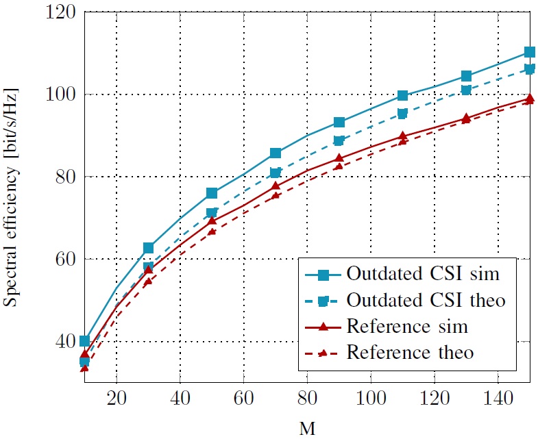
Figure 2: Spectral efficiency for varying values of M

Figure 2 examines the tightness of the proposed analytical lower bound given in Theorem $1$. As can be observed, the proposed lower bound almost overlap with the simulation curve. In addition, we readily see that using outdated CSI with the implicated decrease of training resources increases the SE by $6.91\;\text{bit/s/Hz}$ for $M=50$. This gain attains $11.2\;\text{bit/s/Hz}$ for $M=150$.

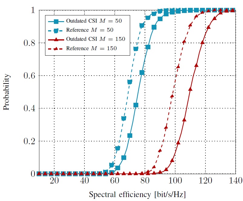
Figure 3: Comparison of the CDFs of spectral efficiency ($N_{G}=30$)

Figure 3 presents a comparison of CDFs of the achievable SE between the reference model and the proposed training scheme for different numbers of antennas at the BS. For $50$ BS antennas, the proposed training scheme achieves a gain in the $5\%$ outage rate of $6\;\text{bit/s/Hz}$. For $150$ antennas, the gain in the $5\%$-outage rate grows to $8\;\text{bit/s/Hz}$. This increase in the performance is mainly due to the reduced training resources which can be used to transmit more data.

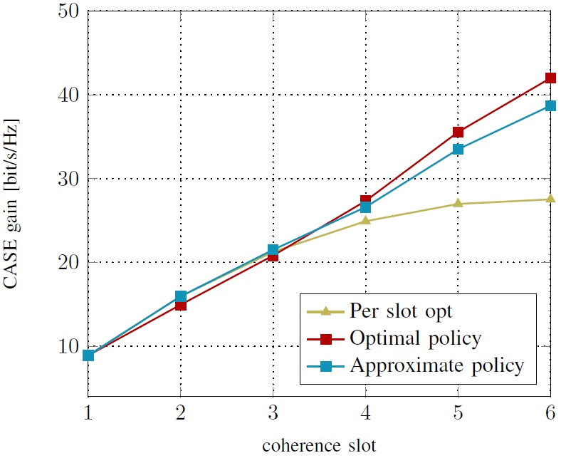
Figure 4: CASE gain for different lower level algorithms

We now investigate the perfomance of the proposed two time scale learning algorithms proposed in sections IV.B, IV.C & IV.D. The performance is evaluated as the difference between the achievable CASE of the considered methods and a classical Massive MIMO TDD protocol.

In Figure 4, we illustrate the performance of the uplink training learning algorithms in sections IV.B & IV.C. The performance of optimal policy (Value iteration) and the approximate one (Algorithm table I) are compared with the case where outdated CSI is used with a per slot optimization. The latter means that the evolution of the correlation between the estimated CSI and the actual channel according to the time dimension is not taken into consideration and the scheduling of copilot groups for uplink training is optimized in order to maximize the ASE at each slot. Figure 4 shows that using value iteration an the approximation algorithm in table I, the gain in CASE is maintained and attains $41.99\;\text{bit/s/Hz}$ and $38.7\;\text{bit/s/Hz}$ respectively, at the final stage of the optimization horizon $H$. However, although per slot optimization achieves also a gain in CASE, we can see that this method performs poorly in comparison with the proposed policies which shows the paramount importance of taking the time dimension into consideration when optimizing uplink training decisions. Finally, due to its good performance, we can deduce that the approximate method (Algorithm table I) represents an efficient low complexity substitute to the more computationally prohibitive DP approach.

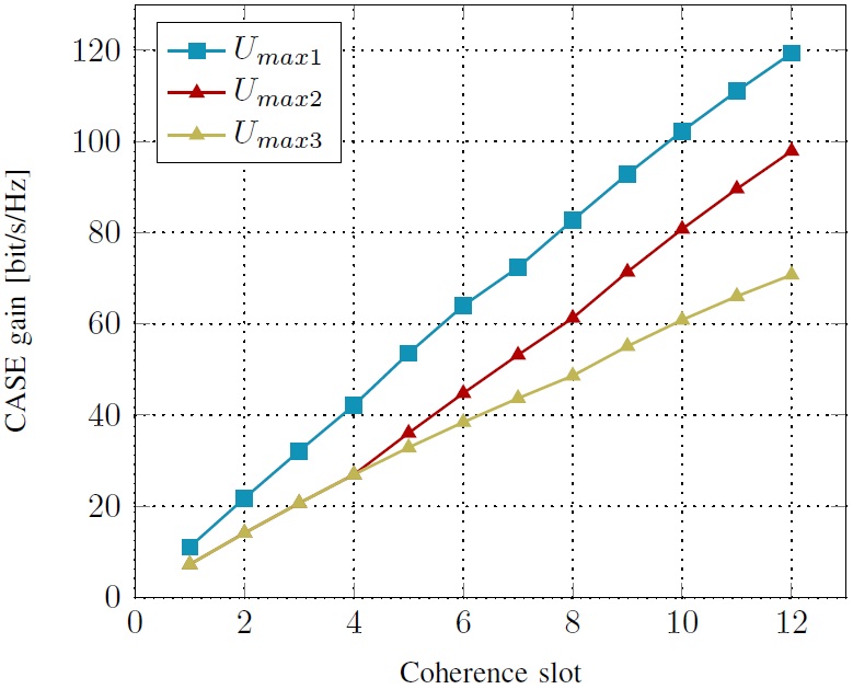
Figure 5: CASE gain for different $U_{max}$ values ($H=4$, $n=0,\ldots,2$, $U_{max1}=N_{G},\;U_{max2}=N_{G}-4\;\text{and}\;U_{max3}=N_{G}-8$

In Figure 5, we illustrate the achievable CASE gain after 3 upper level decision epochs with $H=4$. In this example $3$ values for $U_{max}$ were considered. As can be readily observed, decreasing $U_{max}$ results in lower CASE gain. This is quite intuitive since a lower $U_{max}$ results in more confusion about the users locations. In fact, the CPU commits more errors when inferring users positions from its belief states for lower $U_{max}$ values. Nevertheless, despite the positioning errors the proposed two time scale learning approach is able to provide a considerable CASE gain of $110.26\;\text{bit/s/Hz}$, $97.863\;\text{bit/s/Hz}$ and $70.73\;\text{bit/s/Hz}$ with $U_{max1},\;U_{max2}\;\text{and}\;U_{max3}$ respectively, after $12$ $T_{s}$ slots. These results did not showcase the energy and signaling gains that result from reducing positioning estimation but are sufficient to prove the advantages of allowing the network to proactively plan its uplink training decisions for long time periods.

VI Conclusion

In this paper, we analyzed the performance of an adaptive uplink training scheme for TDD massive MIMO systems, taking into account the actual coherence time of the wireless channels, the impact of channel aging and user mobility. The idea is to adapt the periodicity of CSI estimation based on the actual coherence times. We proposed a two time scale control problem in order to allow the network to learn the best uplink training policy taking into consideration user mobility, channel coherence time and practical signaling overhead limitations. In the fast time scale, the network learns an optimal training policy by choosing which users are requested to send their pilot signals for a predefined optimization horizon. In the slow time scale, owing to practical signaling and processing overhead limitation, the network is required to choose which users are required to feedback their positions, based on their belief states. The present work shows that the aforementioned approach enables to leverage the time evolution of the correlation between the wireless channel and the estimated CSI and provides an impressive increase in the achievable cumulative average spectral efficiency that cannot be obtained otherwise. Future work include the investigation of similar procedures with fairness consideration and user traffic awareness.

Appendix A Appendix

A-A Proof of Theorem 1

The network serves $N_{g}$ copilot groups, $\tau$ of which are scheduled for uplink training. At the reception, each BS uses MRC receivers that are based on the latest CSI estimates. BS $l$ detects the signal of user $g$ in cell $l$ by applying the following filter $u_{gl}(t)=\frac{\hat{g}^{[l]}_{gl}(t-d_{g})}{\lVert\hat{g}^{[l]}_{gl}(t-d_{g})\rVert},t\geq d_{g}$, where $\hat{g}^{[l]}_{gl}(t-d_{g})$ denotes the latest available CSI estimate for user $g$ in cell $l$. Consequently, the detected signal of user $g$ in cell $l$ is given by the following

$$u_{gl}^{\dagger}(t)\frac{Y^{[l]}_{u}(t)}{\sqrt{P_{u}}} =u_{gl}^{\dagger}(t)((\rho^{[l]}_{gl})^{d_{g}}\hat{g}_{gl}^{[l]}(t-d_{g})S_{gl}+\sum_{c\neq l}^{C}(\rho^{[l]}_{gc})^{d_{g}}\hat{g}_{gc}^{[l]}(t-d_{g})S_{gc}+\sum_{k\neq g}^{N_{g}}\sum_{c=1}^{C}g_{kc}^{[l]}(t)S_{kc}$$

$$+\sum_{c=1}^{C}(\rho^{[l]}_{gc})^{d_{g}}\tilde{g}_{gc}^{[l]}(t-d_{g})S_{gc}+\sum_{c=1}^{C}\sum_{j=0}^{d_{g}-1}(\rho^{[l]}_{gc})^{j}\sqrt{\beta_{gc}^{[l]}}\varepsilon_{gc}^{[l]}(t-j)S_{gc}+\frac{W_{u}(t)}{\sqrt{P_{u}}})$$ (37)

$$=u_{il}^{\dagger}(t)(I_{1}(t)+I_{2}(t)+I_{3}(t)),$$

with

$$I_{1}(t) =(\rho^{[l]}_{gl})^{d_{g}}\hat{g}_{gl}^{[l]}(t-d_{g})S_{gl},$$ (38)

$$I_{2}(t) =\sum_{c\neq l}^{C}(\rho^{[l]}_{gc})^{d_{g}}\hat{g}_{gc}^{[l]}(t-d_{g})S_{gc},$$ (39)

$$I_{3}(t) =\sum_{c=1}^{C}(\rho^{[l]}_{gc})^{d_{g}}\tilde{g}_{gc}^{[l]}(t-d_{g})S_{gc}+\sum_{c=1}^{C}\sum_{j=0}^{d_{g}-1}(\rho^{[l]}_{gc})^{j}\sqrt{\beta_{gc}^{[l]}}\varepsilon_{gc}^{[l]}(t-j)S_{gc}+\sum_{k\neq g}^{N_{g}}\sum_{c=1}^{C}g_{kc}^{[l]}(t)S_{kc}+\frac{W_{u}(t)}{\sqrt{P_{u}}}$$ (40)

Equation A-A follows from the fact that $g_{kc}^{[l]}(t)=\sqrt{\beta_{kc}^{[l]}}h_{kc}^{[l]}(t)$, $h_{kc}^{[l]}(t)=\rho_{kc}^{[l]}h_{kc}^{[l]}(t-1)+\varepsilon_{kc}^{[l]}(t)$ for all $t$ and $g_{kc}^{[l]}(t)=\hat{g}_{kc}^{[l]}(t)+\tilde{g}_{kc}^{[l]}(t)$ for all $t$. We note that $I_{1}(\cdot)$ refers to the useful signal, $I_{2}(\cdot)$ represents the impact of pilot contamination and $I_{3}(\cdot)$ regroups the impact of white noise, estimation error, non correlated interference due to users with different pilot sequences and the impact of aging. The instant SE attained by user $g$ in cell $l$ is:

$$R_{g,l}=\left(1-\frac{\tau}{T}\right)\log\left(1+\frac{|u_{gl}^{\dagger}(t)I_{1}(t)|^{2}}{|u_{gl}^{\dagger}(t)I_{2}(t)|^{2}+|u_{gl}^{\dagger}(t)I_{3}(t)|^{2}}\right).$$ (41)

We now define $\overline{R}_{g,l}$ to be the average achievable sum rate of user $g$ in cell $l$, namely,

$$\overline{R}_{g,l}=\mathbb{E}\left(\mathbb{E}\left(\left(1-\frac{\tau}{T}\right)\log\left(1+\frac{|u_{gl}^{\dagger}(t)I_{1}(t)|^{2}}{|u_{gl}^{\dagger}(t)I_{2}(t)|^{2}+|u_{gl}^{\dagger}(t)I_{3}(t)|^{2}}\right)\bigg{|}\hat{g}_{gl}^{[l]}(t-d_{g})\right)\right),$$ (42)

the last equality follows from the law of total expectation. Let us define $\overline{R}_{g,l}^{0}$ such that

$$\overline{R}_{g,l}^{0}=\mathbb{E}\left(\left(1-\frac{\tau}{T}\right)\log\left(1+\frac{|u_{gl}^{\dagger}(t)I_{1}(t)|^{2}}{|u_{gl}^{\dagger}(t)I_{2}(t)|^{2}+|u_{gl}^{\dagger}(t)I_{3}(t)|^{2}}\right)\bigg{|}\hat{g}_{gl}^{[l]}(t-d_{g})\right),$$ (43)

therefore, $\overline{R}_{g,l}=\mathbb{E}(\overline{R}_{g,l}^{0})$. Based on the convexity of $\text{log}(1+\frac{1}{x+a})$, and Jensen’s inequality we obtain the following

$$\overline{R}^{0}_{g,l}\geq\left(1-\frac{\tau}{T}\right)\log\left(1+\frac{|u_{gl}^{\dagger}(t)(\rho_{gl}^{[l]})^{d_{g}}\hat{g}_{gl}^{[l]}(t-d_{g})|^{2}}{\mathbb{E}(|u_{gl}^{\dagger}(t)I_{2}(t)|^{2}|\hat{g}_{gl}^{[l]}(t-d_{g}))+\mathbb{E}(|u_{gl}^{\dagger}(t)I_{3}(t)|^{2}|\hat{g}_{gl}^{[l]}(t-d_{g}))}\right),$$ (44)

since

$$\mathbb{E}(|u_{gl}^{\dagger}(t)I_{1}(t)|^{2}|\hat{g}_{gl}^{[l]}(t-d_{g}))=|u_{gl}^{\dagger}(t)(\rho_{gl}^{[l]})^{d_{g}}\hat{g}_{gl}^{[l]}(t-d_{g})|^{2},$$ (45)

We now aim at computing $\mathbb{E}(|u_{gl}^{\dagger}(t)I_{j}(t)|^{2}|\hat{g}_{gl}^{[l]}(t-d_{g}))\hbox{ for }j=2,3.$ In order to do so, we start by obtaining an alternative expression for $I_{2}(t)$, that is,

$$I_{2}(t) =\sum_{c\neq l}^{C}\hat{g}_{gc}^{[l]}(t-d_{g})S_{gc}=\hat{g}_{gl}^{[l]}(t-d_{g})\sum_{c\neq l}^{C}\frac{\beta_{gc}^{[l]}}{\beta_{gl}^{[l]}}S_{gc},$$ (46)

since $\hat{g}_{gc}^{[l]}(t-d_{g})=\hat{g}_{gl}^{[l]}(t-d_{g})\frac{\beta_{gc}^{[l]}}{\beta_{gl}^{[l]}}$, $I_{2}(t)$ and $\hat{g}_{gl}^{[l]}(t-d_{g})$ are correlated. Consequently, we obtain

$${\mathbb{E}}\left[|u_{gl}^{\dagger}(t)I_{2}(t)|^{2}|\hat{g}_{gl}^{[l]}(t-d_{g})\right]=\left|u_{gl}^{\dagger}(t)\hat{g}^{[l]}_{gl}(t-d_{g})\right|^{2}\sum_{c\neq l}^{C}(\rho^{[l]}_{gc})^{2d_{g}}\frac{\beta^{[l]^{2}}_{gc}}{\beta^{[l]^{2}}_{gl}}.$$ (47)

We will now compute $\mathbb{E}(|u_{gl}^{\dagger}(t)I_{3}(t)|^{2}|\hat{g}_{gl}^{[l]}(t-d_{g}))$. First note that, $I_{3}(t)$ is independent of $\hat{g}_{gl}^{[l]}(t-d_{g})$ and since $u_{gl}^{\dagger}(t)$ has unit norm, we obtain

$$\mathbb{E}(|I_{3}(t)|^{2}) =\mathbb{E}\big{(}\sum_{k\neq g}^{N_{g}}\sum_{c=1}^{C}|g_{kc}^{[l]}(t)|^{2}+\sum_{c=1}^{C}|(\rho_{gc}^{[l]})^{d_{g}}\tilde{g}_{gc}^{[l]}(t-d_{g})|^{2}$$ (48)

$$+\sum_{c=1}^{C}\sum_{j=0}^{d_{g}-1}|\sqrt{\beta_{gc}^{[l]}}(\rho_{gc}^{[l]})^{j}\varepsilon_{gc}^{[l]}(t-j)|^{2}+|\frac{W_{u}(t)}{\sqrt{P_{u}}}|^{2}\big{)},$$

where the equality follows from noting the following four properties; (i) $S_{kc}\cdot S_{ic^{\prime}}=0$ for all $k\neq i$ and all $c,c^{\prime}\in\{0,\ldots,C\}$, (ii) $\mathbb{E}(ZW_{u}(t))=\mathbb{E}(Z)\mathbb{E}(W_{u}(t))=0$ for all random variables $Z$ that are independent of $W_{u}(t)$ (zero mean complex Gaussian noise), (iii) similar to the previous property, $\mathbb{E}(Z\varepsilon_{ic}^{[l]}(t))=\mathbb{E}(Z)\mathbb{E}(\varepsilon_{ic}^{[l]}(t))=0$ for all $Z$ independent of $\varepsilon_{ic}^{[l]}(t)$ (zero mean complex white Gaussian noise) and finally (iv) $g_{kc}^{[l]}$ and $\tilde{g}_{k^{\prime}c^{\prime}}^{[l]}$ are independent for all $(k,c)\neq(k^{\prime},c^{\prime})$.

We now compute the four terms in Equation 48. The last term, i.e.,

$$\mathbb{E}(|W_{u}(t)/\sqrt{P_{u}}|^{2})=\frac{1}{P_{u}}.$$ (49)

We now compute the third term in Equation 48, that is,

$$\mathbb{E}\left(\sum_{c=1}^{C}\sum_{j=0}^{d_{g}-1}|\sqrt{\beta_{gc}^{[l]}}(\rho_{gc}^{[l]})^{j}\varepsilon_{gc}^{[l]}(t-j)|^{2}\right) =\sum_{c=1}^{C}\sum_{j=0}^{d_{g}-1}\beta_{gc}^{[l]}(\rho_{gc}^{[l]})^{2j}(1-(\rho_{gc}^{[l]})^{2})$$ (50)

$$=\sum_{c=1}^{C}\beta_{gc}^{[l]}\frac{1-(\rho_{gc}^{[l]})^{2d_{g}}}{1-(\rho_{gc}^{[l]})^{2}}(1-(\rho_{gc}^{[l]})^{2})$$

$$=\sum_{c=1}^{C}\beta_{gc}^{[l]}({1-(\rho_{gc}^{[l]})^{2d_{g}}}),$$

for the second equality we have used the expression of finite geometric sums since $(\rho_{gc}^{[l]})^{2}<1$ for all $g$ and $c$. Next we compute the second term in Equation 48, namely,

$$\mathbb{E}(\sum_{c=1}^{C}|(\rho_{gc}^{[l]})^{d_{g}}\tilde{g}_{gc}^{[l]}(t-d_{g})|^{2})=\sum_{c=1}^{C}(\rho_{gc}^{[l]})^{2d_{g}}\left(\beta_{gc}^{[l]}-\frac{(\beta_{gc}^{[l]})^{2}}{\frac{1}{P_{p}}+\sum_{b=1}^{C}\beta_{gb}^{[l]}}\right).$$ (51)

the latter is satisfied due to the fact that the variance of $\tilde{g}_{gc}^{[l]}(t-d_{g})$ is given by $\beta_{gc}^{[l]}-\frac{(\beta_{gc}^{[l]})^{2}}{\frac{1}{P_{p}}+\sum_{b=1}^{C}\beta_{gb}^{[l]}}$ for all $g$ and $c$. We are left with the first term in Equation 48, that is,

$$\sum_{k\neq g}^{N_{g}}\sum_{c=1}^{C}\mathbb{E}(|g_{kc}^{[l]}(t)|^{2})=\sum_{k\neq g}^{N_{g}}\sum_{c=1}^{C}\mathbb{E}(|\sqrt{\beta_{kc}^{[l]}}h_{kc}^{[l]}(t)|^{2})=\sum_{k\neq g}^{N_{g}}\sum_{c=1}^{C}\beta_{kc}^{[l]},$$ (52)

Combining all four terms, that is, Equations 49, 50, 51, 52 and 48, we obtain

$${\mathbb{E}}\left[|u_{gl}^{\dagger}(t)I_{3}(t)|^{2}\right] =\sum_{k\neq g}^{N_{g}}\sum_{c=1}^{C}\beta_{kn}^{[l]}+\sum_{c=1}^{C}\beta_{gc}^{[l]}({1-(\rho_{gc}^{[l]})^{2d_{g}}})+\sum_{c=1}^{C}(\rho_{gc}^{[l]})^{2d_{g}}(\beta_{gc}^{[l]}-\frac{(\beta_{gc}^{[l]})^{2}}{\frac{1}{P_{p}}+\sum_{b=1}^{C}\beta_{gb}^{[l]}})$$ (53)

$$=\sum_{k\neq g}^{N_{g}}\sum_{c=1}^{C}\beta_{kc}^{[l]}+\sum_{c=1}^{C}(\beta^{[l]}_{gc}-\rho^{[l]^{2d_{g}}}_{gc}\frac{\beta^{[l]^{2}}_{gc}}{\frac{1}{P_{p}}+\sum_{b=1}^{C}\beta^{[l]}_{gb}})+\frac{1}{P_{u}}.$$

Substituting the results in Equations 53 and 47 in Equation 44, we obtain

$$\overline{R}_{g,l}^{0} \geq\left(1-\frac{\tau}{T}\right)\log\left(1+\frac{(\rho_{gl}^{[l]})^{2d_{g}}|u_{gl}^{\dagger}(t)\hat{g}_{gl}^{[l]}(t-d_{g})|^{2}}{F}\right),$$ (54)

with

$$F= |u_{gl}^{\dagger}(t)\hat{g}_{gl}^{[l]}(t-d_{g})|^{2}\sum_{c\neq l}^{C}(\rho^{[l]}_{gc})^{2d_{g}}\frac{\beta^{[l]^{2}}_{gc}}{\beta^{[l]^{2}}_{gl}}+\sum_{k\neq g}^{N_{g}}\sum_{c=1}^{C}\beta_{kc}^{[l]}+\sum_{c=1}^{C}(\beta^{[l]}_{gc}-\rho^{[l]^{2d_{g}}}_{gc}\frac{\beta^{[l]^{2}}_{gc}}{\frac{1}{P_{p}}+\sum_{b=1}^{C}\beta^{[l]}_{gb}})+\frac{1}{P_{u}}.$$ (55)

From Equation 42 and 55 we obtain

$$\overline{R}_{g,l}=\mathbb{E}(\overline{R}_{g,l}^{0})=\mathbb{E}\left(\left(1-\frac{\tau}{T}\right)\log\left(1+\frac{(\rho_{gl}^{[l]})^{2d_{g}}}{G}\right)\right)\text{, where, }G=\frac{F}{|u_{gl}^{\dagger}(t)\hat{g}_{gl}^{[l]}(t-d_{g})|^{2}}.$$ (56)

Now, we apply Jensen’s inequality to the right hand side (RHS) in Eq. 42, that is,

$$\overline{R}_{g,l} \geq\left(1-\frac{\tau}{T}\right)\log\left(1+\frac{(\rho_{g,l}^{[l]})^{2d_{g}}}{\mathbb{E}(G)}\right),$$ (57)

with

$$\mathbb{E}(G)= \sum_{c\neq l}^{C}(\rho^{[l]}_{gc})^{2d_{g}}\frac{\beta^{[l]^{2}}_{gc}}{\beta^{[l]^{2}}_{gl}}+\mathbb{E}\left(\frac{1}{|u_{gl}^{\dagger}(t)\hat{g}_{gl}^{[l]}(t-d_{g})|^{2}}\right)$$ (58)

$$\cdot\left(\sum_{k\neq g}^{N_{g}}\sum_{c=1}^{C}\beta_{kc}^{[l]}+\sum_{c=1}^{C}(\beta^{[l]}_{gc}-\rho^{[l]^{2d_{g}}}_{gc}\frac{\beta^{[l]^{2}}_{gc}}{\frac{1}{P_{p}}+\sum_{b=1}^{C}\beta^{[l]}_{gb}})+\frac{1}{P_{u}}\right).$$

Note that $\left|u_{gl}^{\dagger}(t)\hat{g}^{[l]}_{gl}(t-d_{g})\right|^{2}$ has a Gamma distribution with parameters $(M,\frac{\beta^{[l]^{2}}_{gl}}{\frac{1}{P_{p}}+\sum_{b=1}^{C}\beta^{[l]}_{gb}})$. Consequently, the mean value of $\frac{1}{\left|u_{gl}^{\dagger}(t)\hat{g}^{[l]}_{gl}(t-d_{g})\right|^{2}}$ is equal to $\frac{1}{(M-1)\times\frac{\beta^{[l]^{2}}_{gl}}{\frac{1}{P_{p}}+\sum_{b=1}^{C}\beta^{[l]}_{gb}}}$. Combining this together with the results in Equations 56 and 58 we obtain the desired lower bound, that is,

$$\overline{R}_{g,l} \geq\left(1-\frac{\tau}{T}\right)\text{log}\left(1+\frac{(M-1)(\beta^{[l]}_{gl})^{2}(\rho^{[l]}_{gl})^{2d_{g}}}{(M-1)I^{p}_{gl}+I^{n}_{gl}}\right),$$ (59)

where $I^{p}_{gl}$ and $I^{n}_{gl}$ are given by

$$I^{p}_{gl}=\sum_{c\neq l}^{C}(\rho^{[l]}_{gc})^{2d_{g}}(\beta^{[l]}_{gc})^{2},\hbox{ and }$$ (60)

$$I^{n}_{gl}=(\frac{1}{P_{p}}+\sum_{b=1}^{C}\beta^{[l]}_{gb})\cdot\left(\sum_{k\neq g}^{N_{g}}\sum_{c=1}^{C}\beta_{kc}^{[l]}+\sum_{c=1}^{C}(\beta^{[l]}_{gc}-\rho^{[l]^{2d_{g}}}_{gc}\frac{\beta^{[l]^{2}}_{gc}}{\frac{1}{P_{p}}+\sum_{b=1}^{C}\beta^{[l]}_{gb}})+\frac{1}{P_{u}}\right).$$ (61)

Summing the achievable SE of all grouped users concludes the proof.

A-B Proof of Theorem $2$

We consider the asymptotic regime where the number of BS antennas $M$ grows large. In this case, the lower bound on the SE of each user $g,l$ converges to the following limit:

$$\left(1-\frac{\tau}{T_{s}}\right)\text{log}\left(1+\frac{\beta^{[l]^{2}}_{gl}\rho^{[l]^{2d_{g}}}_{gl}}{\sum_{b\neq l}^{C}\rho^{[l]^{2d_{g}}}_{gb}\beta^{[l]^{2}}_{gb}}\right).$$

The proposed framework is compared with a reference massive MIMO system where, all scheduled users participate in uplink training. The lower bound on the achievable SE of each user $g,l$, in the reference system, converges to the following:

$$\left(1-\frac{N_{G}}{T_{s}}\right)\text{log}\left(1+\frac{\beta^{[l]^{2}}_{gl}}{\sum_{b\neq l}^{C}\beta^{[l]^{2}}_{gb}}\right).$$ (62)

The aim here, is to improve the achievable SE of each scheduled users. Consequently, the SE of each user in the two considered systems should verify, $\;\forall\;g=1...N_{G},l=1...C$:

$$\left(1-\frac{\tau}{T_{s}}\right)\text{log}\left(1+\frac{\beta^{[l]^{2}}_{gl}\rho^{[l]^{2d_{g}}}_{gl}}{\sum_{b\neq l}^{C}\rho^{[l]^{2d_{g}}}_{gb}\beta^{[l]^{2}}_{gb}}\right)\geq\left(1-\frac{N_{G}}{T_{s}}\right)\text{log}\left(1+\frac{\beta^{[l]^{2}}_{gl}}{\sum_{b\neq l}^{C}\beta^{[l]^{2}}_{gb}}\right),$$ (63)

which is equivalent to the following condition:

$$\frac{\beta^{[l]^{2}}_{gl}\rho^{[l]^{2d_{g}}}_{gl}}{\sum_{b\neq l}^{C}\rho^{[l]^{2d_{g}}}_{gb}\beta^{[l]^{2}}_{gb}}\geq\left(1+\frac{\beta^{[l]^{2}}_{gl}}{\sum_{b\neq l}^{C}\beta^{[l]^{2}}_{gb}}\right)^{\frac{T_{s}-N_{G}}{T_{s}-\tau}}-1.$$

We consider the extreme case where $\rho^{2}_{gl}=\bar{\rho}^{[{min}]^{2}}_{g}$ and $\rho^{2}_{gb}=\bar{\rho}^{[{max}]^{2}}_{{g}},\;\forall b\neq l$. Here $\bar{\rho}^{[{min}]}_{g}$ and $\bar{\rho}^{[{max}]}_{{g}}$ denote respectively the minimum and maximum channel autocorrelation coefficients in group $g$. This means that we assume the worst case scenario for each user. Finally, by considering $SINR^{[\infty]}_{g,l}=\frac{\beta^{[l]^{2}}_{gl}}{\sum_{b\neq l}^{C}\beta^{[l]^{2}}_{gb}}$, we obtain $(14)$ which finishes the proof.

A-C Proof of Theorem $3$

We start by demonstrating that the objective function of problem (34), is submodular. We note that the sum of submodular functions is submodular. Consequently, it is enough to prove the submodularity of $f_{g}$ for a given copilot group $g$, where $f_{g}$ is given by

$$f_{g}(\vec{a}(t_{0}),\ldots,\vec{a}(t_{H-1}),x,\vec{u})=\sum_{t=t_{0}}^{t_{H-1}}\sum_{l=1}^{C}\big{(}1-\frac{1}{T_{s}}\sum_{i=1}^{N_{G}}a_{i}(t)\big{)}\log\big{(}1+\hbox{SINR}_{gl}^{MRC}(\vec{d}(t),x,\vec{u})\big{)},$$ (64)

We consider two sets of action vectors, $\{\vec{a}(t)\in A,,t=t_{0},\ldots,t_{H-1}\}$ and $\{\vec{a}^{\prime}(t)\in A,t=t_{0},\ldots,t_{H-1}\}$ such that, $\forall t=t_{0},\ldots,t_{H-1},\;\sum_{i=1}^{N_{G}}a_{i}(t)\leq\sum_{i=1}^{N_{G}}a^{\prime}_{i}(t),\text{and}\;\forall i=1,\ldots,N_{G},\;a_{i}(h)=1\Rightarrow a^{\prime}_{i}(h)=1$. These two sets of action vectors result, respectively, in two sets of delay vectors $\{\vec{d}(t),t=t_{0},\ldots,t_{H-1}\}$ and $\{\vec{d}^{\prime}(t),t=t_{0},\ldots,t_{H-1}\}$ that can be obtained from $\vec{a}(t)$ and $\vec{a}^{\prime}(t)$ according to (33). In order to prove the submodularity of $f_{g}$, we need to prove that, for a given $h$ and $j$ such that $a_{j}(h)=a^{\prime}_{j}(h)=0$, the marginal values of setting $a_{j}(h)=1$ is higher than that of $a^{\prime}_{j}(h)=1$ ,i.e

$$f_{g}(\vec{a}(t_{0}),\ldots,\vec{a}(h)\oplus a_{j}(h),\ldots,\vec{a}(t_{H-1}),x,\vec{u})-f_{g}(\vec{a}(t_{0}),\ldots,\vec{a}(h),\ldots,\vec{a}(t_{H-1}),x,\vec{u})\geq$$ (65)

$$f_{g}(\vec{a}^{\prime}(t_{0}),\ldots,\vec{a}^{\prime}(h)\oplus a^{\prime}_{j}(h),\vec{a}^{\prime}(t_{H-1}),x,\vec{u})-f_{g}(\vec{a}^{\prime}(t_{0}),\ldots,\vec{a}^{\prime}(h),\ldots,\vec{a}^{\prime}(t_{H-1}),x,\vec{u}).$$

We will distinguish between two cases, $j=g$ and $j\neq g$. For the first case, where $j=g$, the difference between the two marginal values is given by:

$$\Lambda-\Lambda^{\prime}=\sum_{l=1}^{C}\log\big{(}1+\hbox{SINR}_{gl}^{MRC}(0,x,\vec{u})\big{)}\big{(}\frac{\sum_{i=1}^{N_{G}}a^{\prime}_{i}(h)-\sum_{i=1}^{N_{G}}a_{i}(h)}{T_{s}}\big{)}+\big{(}1-\frac{\sum_{i=1}^{N_{G}}a^{\prime}_{i}(h)}{T_{s}}\big{)}$$

$$\log\big{(}1+\hbox{SINR}_{gl}^{MRC}(d^{\prime}_{g}(h),x,\vec{u})\big{)}-\big{(}1-\frac{\sum_{i=1}^{N_{G}}a_{i}(h)}{T_{s}}\big{)}\log\big{(}1+\hbox{SINR}_{gl}^{MRC}(d_{g}(h),x,\vec{u})\big{)}$$

$$+\sum_{t=h+1}^{t_{H-1}}\sum_{l=1}^{C}\big{(}1-\frac{\sum_{i=1}^{N_{G}}a_{i}(t)}{T_{s}}\big{)}\log\big{(}\frac{1+\hbox{SINR}_{gl}^{MRC}(d_{g}(t)-1,x,\vec{u})}{1+\hbox{SINR}_{gl}^{MRC}(d_{g}(t),x,\vec{u})}\big{)}-\big{(}1-\frac{\sum_{i=1}^{N_{G}}a^{\prime}_{i}(t)}{T_{s}}\big{)}$$

$$\log\big{(}\frac{1+\hbox{SINR}_{gl}^{MRC}(d^{\prime}_{g}(t)-1,x,\vec{u})}{1+\hbox{SINR}_{gl}^{MRC}(d^{\prime}_{g}(t),x,\vec{u})}\big{)}$$ (66)

The difference in marginal values is positive as $\log\big{(}\frac{1+\hbox{SINR}_{gl}^{MRC}(d_{g}(t)-1,x,\vec{u})}{1+\hbox{SINR}_{gl}^{MRC}(d_{g}(t),x,\vec{u})}\big{)}$ is decreasing as a function of $d_{g}(t)$. We, now, consider the case where $j\neq g$. In this case, we have

$$\Lambda-\Lambda^{\prime}=\sum_{l=1}^{C}\frac{1}{T_{s}}\log\big{(}\frac{1+\hbox{SINR}_{gl}^{MRC}(d^{\prime}_{g}(h),x,\vec{u})}{1+\hbox{SINR}_{gl}^{MRC}(d_{g}(h),x,\vec{u})}\big{)}$$ (67)

From the definition of $\vec{a}(h)$ and $\vec{a}^{\prime}(h)$, we have $\sum_{i=1}^{N_{G}}a_{i}(h)\leq\sum_{i=1}^{N_{G}}a^{\prime}_{i}(h)$.
Hence $\hbox{SINR}_{gl}^{MRC}(d^{\prime}_{g}(h),x,\vec{u})\geq\hbox{SINR}_{gl}^{MRC}(d_{g}(h),x,\vec{u})$ and the difference in marginal values is also positive, in this case. Consequently, $f_{g}$ is submodular. Concerning the matroid constraints, let us consider the ground set $G=\{v_{1t_{1}},\ldots,v_{N_{G}t_{1}},\ldots,v_{1t_{H-1}},\ldots,v_{N_{G}t_{H-1}}\}$, where each element $v_{gt}$ represents the scheduling of copilot group $g$ for training at slot $t$. It is clear that the constraints $(35)$ form a partition matroid on $G$ [30]. Consequently, problem (34) is a maximization of a submodular function subject to matroid constraints.

References

• [1] Akhil Gupta, Rakesh Kumar Jha, A survey of 5G network: Architecture and emerging technologies, IEEE access (3), pp. 1206–1232, 2015.
• [2] T. L. Marzetta, , Noncooperative cellular wireless with unlimited numbers of base station antennas, IEEE Transactions on Wireless Communications, vol. 9, no. 11, pp. 3590-3600, November 2010.
• [3] H. Q. Ngo, E. G. Larsson, and T. L. Marzetta, Energy and spectral efficiency of very large multiuser MIMO systems, IEEE Trans. Commun., 2012, submitted. [Online]. Available: http://arxiv.org/abs/1112.3810
• [4] B. Gopalakrishnan and N. Jindal, An analysis of pilot contamination on multi-user MIMO cellular systems with many antennas, in Proc. Int. Workshop Signal Process. Adv. Wireless Commun., June 2011, pp. 381-385.
• [5] A. Ashikhmin and T. L. Marzetta, Pilot contamination and precoding in multi-cell large scale antenna systems, in Proc. IEEE Int. Symp. Inf. Theory, Cambridge, MA, 2012, pp. 1142-1146.
• [6] L. Thiele, M. Olbrich, M. Kurras, and B. Matthiesen, Channel aging effects in CoMP transmission: gains from linear channel prediction,in Proc. of Asilomar Conf. Signals Systems Computers, Nov. 2011, pp. 1924-1928.
• [7] K. T. Truong and R. W. Heath Jr., Effects of channel aging in massive MIMO systems, J. Commun. Netw., vol. 16, no. 4, pp. 338-351, Aug. 2013.
• [8] A. K. Papazafeiropoulos and T. Ratnarajah, Linear precoding for downlink massive MIMO with delayed CSIT and channel prediction, in Proc. IEEE WCNC, Apr. 2014, pp. 809-914.
• [9] A. K. Papazafeiropoulos and T. Ratnarajah, Uplink performance of massive MIMO subject to delayed CSIT and anticipated channel prediction, in Proc. IEEE ICASSP, May 2014, pp. 3162-3165.
• [10] Chuili Kong, Caijun Zhong, Anastasios K. Papazafeiropoulos, Michail Matthaiou and Zhaoyang Zhang, Sum-Rate and Power Scaling of Massive MIMO Systems with Channel Aging, Information Theory (ISIT), 2015.
• [11] Thang X. Vu, Trinh Anh Vu, Symeon Chatzinotas and Bjorn Ottersten, Spectral-Efficient Model for Multiuser Massive MIMO: Exploiting User Velocity, IEEE International Conference on Communications (ICC), 2017.
• [12] S. Hajri and M. Assaad, M. Larrañaga, Enhancing massive MIMO: A new approach for Uplink training based on heterogeneous coherence times, http://www.l2s.centralesupelec.fr/perso/salah.hajri/publications
• [13] Issam Toufik, Stefania Sesia, LTE: The UMTS Long Term Evolution, John Wiley & Sons, 2011.
• [14] H. S. Chang, P. J. Fard, S. I. Marcus, and M. Shayman, Multitime scale markov decision processes, Automatic Control, IEEE Transactions on, vol. 48, jun 2003.
• [15] LaValle, S. M.,Planning Algorithms, University of Illinois 1999-2004.
• [16] W. Jakes and D. Cox, Microwave Mobile Communications, Wiley-IEEE Press, 1994.
• [17] T. Y. Young and T. W. Calvert, Classification, estimation and pattern recognition, American Elsevier Publishing Company, 1974.
• [18] I. M. Taylor and M. A. Labrador, Improving the Energy Consumption in Mobile Phones by Filtering Noisy GPS Fixes with Modified Kalman Filters, Proceedings of IEEE Wireless Communications and Networking Conference, March 28-31 2011, pp. 2006-2011.
• [19] D. BRAZIUNAS, POMDP solution methods. Tech. rep., 2003
• [20] Tamás Szálka, Péter Fülöp and Sándor Imre, General mobility modeling and location prediction based on markovian approach constructor framework, Periodica Polytechnica Electrical Engineering (Archives), 55, 2011.
• [21] Making 5G NR a reality, Qualcomm Technologies Inc , December 2016.
• [22] J. Lee, V. Mirrokni, V. Nagarajan and M. Sviridenko. Maximizing Non-Monotone Submodular Functions under Matroid and Knapsack Constraints. IBM Research Report RC24679. 2008.
• [23] Yang Li, Young-Han Nam, Boon Loong Ng, Jianzhong Zhang, A non-asymptotic throughput for massive MIMO cellular uplink with pilot reuse, Global Communications Conference (GLOBECOM), 2012 IEEE.
• [24] G. Calinescu, C. Chekuri, M. Pal, and J. Vondrak, Maximizing a submodular set function subject to a matroid constraint, Integer programming and combinatorial optimization, pp. 182-196, 2007.
• [25] D. Bertsekas. Dynamic Programming and Optimal Control. Athena Scientific. 1995.
• [26] Geoff Varrall, 5G Spectrum and Standards, Artech House, 31 mai 2016
• [27] Aberdeen, D. A survey of approximate methods for solving partially observable Markov decision processes, Technical report, Research School of Information Science and Engineering, Australia National University, 2002.
• [28] I. Nourbakhsh, R. Powers, and S. Birchfield, DERVISH an office-navigating robot, AI Magazine 16, pp. 53-60, 1995.
• [29] S. E. Hajri, M. Assaad, and G. Caire, Scheduling in massive MIMO: User clustering and pilot assignment, in Proc. Allerton Conference on Communication, Control, and Computing, sep 2016.
• [30] J. G. Oxley, Matroid theory, Oxford Science Publications. The Clarendon Press, Oxford University Press, New York, 1992.