Thermodynamics of the kagome-lattice Heisenberg antiferromagnet with arbitrary spin $S$.

Abstract

We use a second-order rotational invariant Green’s function method (RGM) and the high-temperature expansion (HTE) to calculate the thermodynamic properties, of the kagome-lattice spin-$S$ Heisenberg antiferromagnet with nearest-neighbor exchange $J$. While the HTE yields accurate results down to temperatures of about $T/S(S+1)\sim J$, the RGM provides data for arbitrary $T\geq 0$. For the ground state we use the RGM data to analyze the $S$-dependence of the excitation spectrum, the excitation velocity, the uniform susceptibility, the spin-spin correlation functions, the correlation length, and the structure factor. We found that the so-called $\sqrt{3}\times\sqrt{3}$ ordering is more pronounced than the $q=0$ ordering for all values of $S$. In the extreme quantum case $S=1/2$ the zero-temperature correlation length is only of the order of the nearest-neighbor separation. Then we study the temperature dependence of several physical quantities for spin quantum numbers $S=1/2,1,\dots,7/2$. As increasing $S$ the typical maximum in the specific heat and in the uniform susceptibility are shifted towards lower values of $T/S(S+1)$ and the height of the maximum is growing. The structure factor ${\cal S}(\mathbf{q})$ exhibits two maxima at magnetic wave vectors $\mathbf{q}={\mathbf{Q}_{i}},i=0,1,$ corresponding to the $q=0$ and $\sqrt{3}\times\sqrt{3}$ state. We find that the $\sqrt{3}\times\sqrt{3}$ short-range order is more pronounced than the $q=0$ short-range order for all temperatures $T\geq 0$. For the spin-spin correlation functions, the correlation lengths and the structure factors, we find a finite low-temperature region $0\leq T<T^{*}\approx a/S(S+1)$, $a\approx 0.2$, where these quantities are almost independent of $T$.

I Introduction

One of the most prominent and at the same time challenging spin models with a frustration induced highly degenerated classical ground state (GS) manifold is the kagome Heisenberg antiferromagnet (KHAF) Zeng and Elser (1990); Chalker et al. (1992); Harris et al. (1992); Singh and Huse (1992); Reimers and Berlinsky (1993); Elstner et al. (1993); Elstner and Young (1994); Henley and Chan (1995); Nakamura and Miyashita (1995); Tomczak and Richter (1996); Waldtmann et al. (1998); Yu and Feng (2000); Sindzingre et al. (2000); García-Adeva and Huber (2001); Bernhard et al. (2002); Schmalfuß et al. (2004); Misguich and Bernu (2005); Singh and Huse (2007); Li et al. (2007); Rigol et al. (2007); Zhitomirsky (2008); Jiang et al. (2008); Läuchli and Lhuillier (2009); Evenbly and Vidal (2010); Götze et al. (2011); Nakano and Sakai (2011); Iqbal et al. (2011); Yan et al. (2011); Läuchli et al. (2011); Depenbrock et al. (2012); Rousochatzakis et al. (2013); Iqbal et al. (2013); Rousochatzakis et al. (2014); Xie et al. (2014); Lohmann et al. (2014); Munehisa (2014); Kolley et al. (2015); Götze and Richter (2015); Changlani and Läuchli (2015); Liu et al. (2015); Picot and Poilblanc (2015); Nishimoto and Nakamura (2015); Liu et al. (2016); Shimokawa and Kawamura (2016); Oitmaa and Singh (2016); Götze and Richter (2016); Läuchli et al. (2016); He et al. (2017); Liao et al. (2017); P. and Singh (2017); Chen et al. (2017). This degeneracy is lifted by fluctuations (order from disorder mechanism) Villain et al. (1980); Shender (1982); Henley and Chan (1995). Particular attention has been paid to the extreme quantum spin-half case [Waldtmann et al., 1998; Yu and Feng, 2000; Sindzingre et al., 2000; Bernhard et al., 2002; Schmalfuß et al., 2004; Singh and Huse, 2007; Li et al., 2007; Zhitomirsky, 2008; Jiang et al., 2008; Läuchli and Lhuillier, 2009; Evenbly and Vidal, 2010; Götze et al., 2011; Nakano and Sakai, 2011; Iqbal et al., 2011; Yan et al., 2011; Läuchli et al., 2011; Depenbrock et al., 2012; Rousochatzakis et al., 2013; Iqbal et al., 2013; Rousochatzakis et al., 2014; Xie et al., 2014; Lohmann et al., 2014; Kolley et al., 2015; Götze and Richter, 2015, 2016; Läuchli et al., 2016; He et al., 2017; Liao et al., 2017; P. and Singh, 2017; Chen et al., 2017]. Although, there is consensus on the absence of magnetic long-range order (LRO) the nature of the spin-liquid GS is still under debate. Meanwhile also for spin quantum number $S=1$ there is evidence that the KHAF does not exhibit magnetic LRO Götze et al. (2011); Götze and Richter (2015); Changlani and Läuchli (2015); Liu et al. (2015); Picot and Poilblanc (2015); Nishimoto and Nakamura (2015). Recently it has been argued that there is a route to magnetic GS LRO in the KHAF as increasing the spin quantum number to $S\geq 3/2$, see Götze et al. (2011); Götze and Richter (2015); Oitmaa and Singh (2016); Liu et al. (2016).

Except the theoretical work there is also a large activity on the experimental side. Among the $S=1/2$ kagome compounds, Herbertsmithite ZnCu₃(OH)₆Cl₂ is a promising candidate for a spin liquid, see Mendels et al. (2007); Helton et al. (2007); Hiroi et al. (2009); de Vries et al. (2009); Wulferding et al. (2010); Han et al. (2012). Examples for kagome magnets with higher spin $S$ are deuteronium jarosite (D₃O)Fe₃(SO₄)₂(OD)₆ with spin $S=5/2$, see Fåk et al. (2007), and the recently studied Cr-Jarosite KCr₃(OH)₆(SO₄)₂ with spin $S=3/2$, see Okubo et al. (2017).

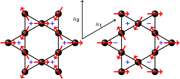
Figure 1: Illustration of the two most relevant classical states. Left: $q=0$ state with magnetic wave vector $\mathbf{Q}_{0}=(2\pi/\sqrt{3},0)$. Right: $\sqrt{3}\times\sqrt{3}$ state with magnetic wave vector $\mathbf{Q}_{1}=(0,4\pi/3)$. "$+$" and "$-$" symbols denote plaquettes of different vector spin chirality. The arrows indicate the basis vectors $\mathbf{a}_{1}$ and $\mathbf{a}_{2}$.

Due to the order from disorder mechanism two different coplanar states may be selected by fluctuations: (i) The so called $q=0$ state with a corresponding magnetic wave vector $\mathbf{Q}_{0}=(2\pi/\sqrt{3},0)$ (Fig. 1, left), which has a magnetic unit cell that is identical to the geometrical one. (ii) The so called $\sqrt{3}\times\sqrt{3}$ state (Fig. 1, right) with a corresponding magnetic wave vector $\mathbf{Q}_{1}=(0,4\pi/3)$ which has a three times larger unit cell, cf. e.g., Zhitomirsky (2008). Moreover, both states are characterized by different vector chirality patterns, see Fig. 1. The selection of one of these states is a subtle issue and depends on spin quantum number, anisotropy etc., see, e.g., Sachdev (1992); Chubukov (1992); Henley and Chan (1995); Götze et al. (2011); Chernyshev and Zhitomirsky (2014, 2015); Götze and Richter (2015, 2016). While for the widely studied GS properties a plethora of many-body methods are available, the tool box for the calculation of finite-temperature properties of highly frustrated quantum magnets is sparse. Here we use two universal approaches suitable to calculate thermodynamic quantities of Heisenberg quantum spin systems of arbitrary lattice geometry, namely the Green-function technique Gasser et al. (2001); Nolting and Ramakanth (2009); Fröbrich and Kuntz (2006) and the high-temperature expansion Elstner et al. (1993); Elstner and Young (1994); Rosner et al. (2003); Singh and Oitmaa (2012); Bernu et al. (2013); Oitmaa et al. (2006); Bernu and Misguich (2001); Misguich and Bernu (2005); Bernu and Lhuillier (2015); Schmidt et al. (2011); Lohmann et al. (2014); Richter et al. (2015); Schmidt et al. (2017); P. and Singh (2017).

We study the kagome lattice with antiferromagnetic ($J>0$) nearest-neighbor interaction

$$\hat{H}=J\sum_{\langle m\alpha,n\beta\rangle}\bm{\hat{S}}_{m\alpha}\bm{\hat{S}}_{n\beta}\;,\;\bm{\hat{S}}_{m\alpha}^{2}=S(S+1),$$ (1)

where the Greek indices ($\alpha,\beta=1,2,3$) run over the spins in a geometrical unit cell (that contains three sites) and the latin indices $n$ and $m$ label the unit cells given by the basis vectors $\mathbf{a}_{1}=(0,2)$ and $\mathbf{a}_{2}=(\sqrt{3},1)$.

The paper is organized as follows: In Sec. II we briefly illustrate the applied methods. In Sec. III.1 we describe the properties of the model at zero temperature, followed by the discussion of finite-temperature properties of the model in Sec. III.2. In Sec. IV we summarize our findings.

II Methods

II.1 Rotation-invariant Green’s function method (RGM)

A rotation-invariant formalism of the Green’s function method was first introduced by Kondo and Yamaji Kondo and Yamaji (1972) to describe short-range order (SRO) of the one-dimensional $S=1/2$ Heisenberg ferromagnet at $T>0$. They decoupled the hierarchy of equation of motions in second order, i.e., one step beyond the usual random-phase approximation (RPA) Tyablikov (1967); Gasser et al. (2001); Nolting and Ramakanth (2009) and introduced rotational invariance by setting $\langle\hat{S}^{z}_{i}\rangle=0$ in the equations of motions. Within this rotation-invariant scheme possible magnetic LRO is described by the long-range part in the two-point spin correlators. Furthermore, the approximation made by the decoupling of higher-order correlators is improved by introducing so-called vertex parameters, see below. In the following decades the rotation-invariant Green’s function method (RGM) was further elaborated to include arbitrary spin $S$, antiferromagnetic spin systems including frustrated ones and also more complex spin-lattices with non-primitive unit cells Rhodes and Scales (1973); Shimahara and Takada (1991); Suzuki et al. (1994); Barabanov and Beresovsky (1994); Winterfeldt and Ihle (1997); Ihle et al. (1999); Yu and Feng (2000); Siurakshina et al. (2001); Bernhard et al. (2002); Schmalfuß et al. (2004, 2006, 2005); Junger et al. (2005, 2009); Härtel et al. (2008, 2010, 2011a, 2011b, 2013); Antsygina et al. (2008); Mikheyenkov et al. (2013); A. A. Vladimirov et al. (2014); Müller et al. (2015); Mikheyenkov et al. (2016); A. A. Vladimirov et al. (2017); Müller et al. (2017a, b). At the present time the RGM is a well established method and has been successfully used in numerous recent publications on the theory of frustrated spin systems Yu and Feng (2000); Siurakshina et al. (2001); Bernhard et al. (2002); Schmalfuß et al. (2004, 2006, 2005); Härtel et al. (2008, 2010, 2011a, 2011b, 2013); Müller et al. (2015); Junger et al. (2005, 2009); Mikheyenkov et al. (2013, 2016); Müller et al. (2017a, b).

The early papers using the RGM Yu and Feng (2000); Bernhard et al. (2002); Schmalfuß et al. (2004) to study the KHAF were restricted to the spin-$1/2$ case and used a simple minimal version of the RGM, see below. In the present paper we extend the RGM approach to arbitrary values of the spin quantum number $S\geq 1$ and improve the previous RGM studies going beyond the minimal version by introducing one more vertex parameter. Moreover, we provide a more comprehensive analysis of the thermodynamic quantities by considering, e.g. the temperature dependence of the structure factor and correlation lengths.

The basic quantity that has to be determined within the RGM is the (retarded) Green’s function $\langle\langle\hat{S}_{\mathbf{q}\alpha}^{+};\hat{S}_{\mathbf{\mathbf{q}\beta}}^{-}\rangle\rangle_{\omega}$, which is related to the dynamic wavelength-dependent susceptibility $\langle\langle\hat{S}_{\mathbf{q}\alpha}^{+};\hat{S}_{\mathbf{\mathbf{q}\beta}}^{-}\rangle\rangle_{\omega}=-\chi^{+-}_{\alpha\beta\mathbf{q}}(\omega)$. To determine $\langle\langle\hat{S}_{\mathbf{q}\alpha}^{+};\hat{S}_{\mathbf{\mathbf{q}\beta}}^{-}\rangle\rangle_{\omega}$ we use the equation of motion (EoM) up to second order,

$$\omega\langle\langle\hat{S}_{\mathbf{q}\alpha}^{+};\hat{S}_{\mathbf{\mathbf{q}\beta}}^{-}\rangle\rangle_{\omega} = \langle[\hat{S}_{\mathbf{q}\alpha}^{+},\hat{S}_{\mathbf{\mathbf{q}\beta}}^{-}]_{-}\rangle+\langle\langle\textrm{i}\dot{\hat{S}}_{\mathbf{q}\alpha}^{+};\hat{S}_{\mathbf{\mathbf{q}\beta}}^{-}\rangle\rangle_{\omega},$$

$$\omega\langle\langle\textrm{i}\dot{\hat{S}}_{\mathbf{q}\alpha}^{+};\hat{S}_{\mathbf{\mathbf{q}\beta}}^{-}\rangle\rangle_{\omega} = \langle[\textrm{i}\dot{\hat{S}}_{\mathbf{q}\alpha}^{+},\hat{S}_{\mathbf{\mathbf{q}\beta}}^{-}]_{-}\rangle-\langle\langle\ddot{\hat{S}}_{\mathbf{q}\alpha}^{+};\hat{S}_{\mathbf{\mathbf{q}\beta}}^{-}\rangle\rangle_{\omega}.$$ (2)

Naturally, for an interacting many-body problem more complicated (i.e., higher-order) Green’s functions appear in the EoM. It is in order to mention here that the RPA, that can be obtained by applying the EoM only once (first line in Eq. (2)), has the disadvantage that only phases with magnetic LRO can be described properly, since the Green’s function is proportional to magnetic order parameters Tyablikov (1967); Gasser et al. (2001); Nolting and Ramakanth (2009). In contrast, SRO can be adequately described by the RGM due to including the next order in the EoM, see the second line in Eq. (2). The operator $\ddot{\hat{S}}_{\mathbf{q}\alpha}^{+}$ appearing in second-order contains several combinations of three-spin operators. These products of three-spin operators are simplified by the decoupling scheme along the lines of, e.g., Suzuki et al. (1994); Junger et al. (2009); Härtel et al. (2011a); Müller et al. (2017b) which can be sketched as follows:

$$\hat{S}_{A}^{-}\hat{S}_{B}^{+}\hat{S}_{C}^{+} \rightarrow \alpha_{AB}c^{+-}_{AB}\hat{S}_{C}^{+}+\alpha_{AC}c^{+-}_{AC}S_{B}^{+},$$ (3)

$$\hat{S}_{A}^{z}\hat{S}_{B}^{z}\hat{S}_{C}^{+} \rightarrow \frac{1}{2}\alpha_{AB}c^{+-}_{AB}\hat{S}_{C}^{+},$$

$$\hat{S}_{A}^{z}\hat{S}_{A}^{z}\hat{S}_{B}^{+} \rightarrow c^{zz}_{AA}\hat{S}_{B}^{+}=\frac{1}{2}c^{+-}_{AA}\hat{S}_{B}^{+},$$

$$\hat{S}_{A}^{-}\hat{S}_{B}^{+}\hat{S}_{A}^{+} \rightarrow c^{+-}_{AA}\hat{S}_{B}^{+}+\lambda_{AB}c^{+-}_{AB}\hat{S}_{A}^{+},$$

$$\hat{S}_{A}^{z}\hat{S}_{B}^{z}\hat{S}_{A}^{+} \rightarrow \frac{1}{2}\lambda_{AB}c^{+-}_{AB}\hat{S}_{A}^{+},$$

$$\hat{S}_{A}^{-}\hat{S}_{B}^{+}\hat{S}_{B}^{+} \rightarrow 2\lambda_{AB}c^{+-}_{AB}\hat{S}_{B}^{+},$$

where $A\neq B\neq C\neq A$ are sites of the kagome lattice, $c^{+-}_{AB}=\langle\hat{S}_{A}^{+}\hat{S}_{B}^{-}\rangle$ and the conservation of total $S^{z}$ is implied, i.e., $c^{+z}_{AB}=c^{-z}_{AB}=0$.

In Eq. (3) two classes of so-called vertex parameters, $\alpha_{AB}$ and $\lambda_{AB}$, are introduced to improve the approximation made by the decoupling. The parameter $\alpha_{AB}$ enters the decoupling scheme if all sites are different from each other, see lines 1 and 2 in Eq. (3). In line 3 of Eq. (3) the correlation $\langle\hat{S}_{A}^{+}\hat{S}_{A}^{-}\rangle$ is determined by using the sum rule (operator identity) $\hat{\mathbf{S}}^{2}=\hat{S}^{+}\hat{S}^{-}-\hat{S}^{z}+(\hat{S}^{z})^{2}$, i.e., due to $\langle\hat{S}^{z}\rangle=0$ within the RGM we have $3\langle(\hat{S}^{z})^{2}\rangle=\langle\hat{\mathbf{S}}^{2}\rangle=\langle\hat{S}^{+}\hat{S}^{-}\rangle+\langle(\hat{S}^{z})^{2}\rangle$ and finally $\langle\hat{S}_{A}^{+}\hat{S}_{A}^{-}\rangle=\frac{2}{3}S(S+1)$. The other class of vertex parameters, $\lambda_{AB}$, present in lines 4, 5 and 6 of Eq. (3) appears only for $S>1/2$ if two sites coincide and the remaining correlation function cannot be obtained by an operator identity.

Then the EoM reads

$$(\omega^{2}\mathbb{I}-F_{\mathbf{q}})\chi^{+-}_{\mathbf{q}}(\omega) = -M_{\mathbf{q}},$$ (4)

where $M_{\mathbf{q}}$ (moment matrix), $F_{\mathbf{q}}$ (frequency matrix) and $\chi_{\mathbf{q}}$ (susceptibility matrix) are hermitian 3$\times$3-matrices and $\mathbb{I}$ is the identity matrix. Performing corresponding calculations as described above the components $M^{\alpha\beta}_{\mathbf{q}}=\langle[\textrm{i}\dot{\hat{S}}_{\mathbf{q}\alpha}^{+},\hat{S}_{\mathbf{q}\beta}^{-}]\rangle$ of the moment matrix are obtained as

$$M_{\mathbf{q}}=$$ (5)

$$4Jc_{1,0} \left(\begin{array}[]{ccc}-2&\cos(\frac{\sqrt{3}q_{x}-q_{y}}{2})&\cos(q_{y})\\ \cos(\frac{\sqrt{3}q_{x}-q_{y}}{2})&-2&\cos(\frac{\sqrt{3}q_{x}+q_{y}}{2})\\ \cos(q_{y})&\cos(\frac{\sqrt{3}q_{x}+q_{y}}{2})&-2\end{array}\right).$$ (8)

The elements of frequency matrix of the spin excitations

$$F_{\mathbf{q}}=\left(\begin{array}[]{ccc}F_{\mathbf{q}}^{1,1}&F_{\mathbf{q}}^{1,2}&F_{\mathbf{q}}^{1,3}\\ F_{\mathbf{q}}^{1,2}&F_{\mathbf{q}}^{2,2}&F_{\mathbf{q}}^{2,3}\\ F_{\mathbf{q}}^{1,3}&F_{\mathbf{q}}^{2,3}&F_{\mathbf{q}}^{3,3}\end{array}\right),$$ (12)

are given by

$$\frac{3}{2}J^{-2}F_{\mathbf{q}}^{1,1}=6\tilde{\lambda}_{1,0}+6\tilde{\alpha}_{1,1}+6\tilde{\alpha}_{2,0}+4S(S+1)$$ (13)

$$+3\left(\cos\left(\sqrt{3}q_{x}-q_{y}\right)+\cos(2q_{y})+2\right)\tilde{\alpha}_{1,0},$$

$$\frac{3}{4}J^{-2}F_{\mathbf{q}}^{2,2}=3\tilde{\lambda}_{1,0}+3\tilde{\alpha}_{1,1}+3\tilde{\alpha}_{2,0}+2S(S+1)$$

$$+3\left(\cos\left(\sqrt{3}q_{x}\right)\cos(q_{y})+1\right)\tilde{\alpha}_{1,0},$$

$$\frac{3}{2}J^{-2}F_{\mathbf{q}}^{3,3}=6\tilde{\lambda}_{1,0}+6\tilde{\alpha}_{1,1}+6\tilde{\alpha}_{2,0}+4S(S+1)$$

$$+3\left(\cos\left(\sqrt{3}q_{x}+q_{y}\right)+\cos(2q_{y})+2\right)\tilde{\alpha}_{1,0},$$

$$(\sqrt{2}J)^{-2}F_{\mathbf{q}}^{1,2} = \cos\left(\frac{1}{2}\left(\sqrt{3}q_{x}+3q_{y}\right)\right)\tilde{\alpha}_{1,0}$$

$$- \cos\left(\frac{1}{2}\left(\sqrt{3}q_{x}-q_{y}\right)\right)\left(\tilde{\lambda}_{1,0}+3\tilde{\alpha}_{1,0}+\tilde{\alpha}_{1,1}+\tilde{\alpha}_{2,0}+\frac{2}{3}S(S+1)\right),$$

$$(\sqrt{2}J)^{-2}F_{\mathbf{q}}^{1,3} = \cos\left(\sqrt{3}q_{x}\right)\tilde{\alpha}_{1,0}-\cos(q_{y})\left(\tilde{\lambda}_{1,0}+3\tilde{\alpha}_{1,0}+\tilde{\alpha}_{1,1}+\tilde{\alpha}_{2,0}+\frac{2}{3}S(S+1)\right),$$

$$(\sqrt{2}J)^{-2}F_{\mathbf{q}}^{2,3} = \cos\left(\frac{1}{2}\left(\sqrt{3}q_{x}-3q_{y}\right)\right)\tilde{\alpha}_{1,0}$$

$$- \cos\left(\frac{1}{2}\left(\sqrt{3}q_{x}+q_{y}\right)\right)\left(\tilde{\lambda}_{1,0}+3\tilde{\alpha}_{1,0}+\tilde{\alpha}_{1,1}+\tilde{\alpha}_{2,0}+\frac{2}{3}S(S+1)\right),$$

where we have used the abbreviations

$$\tilde{\alpha}_{i,j}=\alpha_{i,j}c_{i,j},\quad\tilde{\lambda}_{i,j}=\lambda_{i,j}c_{i,j},$$ (15)

and lattice symmetry is used to identify equivalent correlators. The indices $i,j$ indicate lattice sites separated by the vector $\mathbf{R}_{i,j}=\mathbf{r}_{i}-\mathbf{r}_{j}=i\mathbf{a_{1}}/2+j\mathbf{a_{2}}/2$, i.e., $c_{ij}\equiv\langle\hat{S}^{+}_{\mathbf{0}}\hat{S}^{-}_{\mathbf{R}_{i,j}}\rangle$. Their common eigenvectors $|{\gamma\mathbf{q}}\rangle$ and their eigenvalues ($M_{\mathbf{q}}|{\gamma\mathbf{q}}\rangle=m_{\gamma\mathbf{q}}|{\gamma\mathbf{q}}\rangle,F_{\mathbf{q}}|{\gamma\mathbf{q}}\rangle=\omega^{2}_{\gamma\mathbf{q}}|{\gamma\mathbf{q}}\rangle$, with $\gamma=1,2,3$) are needed to solve a system of self-consistent equations. The square-root of the eigenvalues of the frequency matrix $F_{\mathbf{q}}$ can be identified as the branches $\omega_{\gamma\mathbf{q}}$, $\gamma=1,2,3$, of the excitation spectrum.

Finally, the dynamic wavelength-dependent susceptibility reads

$$\chi^{+-}_{\mathbf{q\alpha\beta}}(\omega)=-\sum_{\gamma}\frac{m_{\gamma\mathbf{q}}}{\omega^{2}-\omega^{2}_{\gamma\mathbf{q}}}\langle\alpha|{\gamma\mathbf{q}}\rangle\langle{\gamma\mathbf{q}}|\beta\rangle$$ (16)

and the static $\mathbf{q}$-dependent susceptibility is given by

$$\chi_{\mathbf{q}}=\lim_{\omega\rightarrow 0}\frac{1}{2n_{\rm uc}}\sum_{\alpha,\beta}\chi^{+-}_{\mathbf{q}\alpha\beta}(\omega),$$ (17)

where $n_{\rm uc}=3$ is the number of sites in the geometric unit cell. The correlation functions are obtained by applying the spectral theorem

$$c_{m\alpha,n\beta} = \frac{1}{\mathcal{N}}\sum_{\mathbf{q}}c_{\mathbf{q}\alpha\beta}\cos(\mathbf{q}\mathbf{r}_{m\alpha,n\beta}),$$ (18)

with

$$c_{\mathbf{q}\alpha\beta} = \sum_{\gamma}\frac{m_{\gamma\mathbf{q}}}{2\omega_{\gamma\mathbf{q}}}(1+2n(\omega_{\gamma\mathbf{q}}))\langle\alpha|{\gamma\mathbf{q}}\rangle\langle{\gamma\mathbf{q}}|\beta\rangle,$$ (19)

where $\mathcal{N}$ is the number of unit cells and $n(\omega_{\gamma\mathbf{q}})$ is the Bose-Einstein distribution function. At the $\Gamma$ point ($\mathbf{q}=\mathbf{0}$) the eigenvectors have the very simple form $|{1\mathbf{0}}\rangle=(1,0,-1)/\sqrt{2}$, $|{2\mathbf{0}}\rangle=(1,-2,1)/\sqrt{6}$, and $|{3\mathbf{0}}\rangle=(1,1,1)/\sqrt{3}$.

After straightforward calculations we get

$$m_{1{\bf q}} = -12Jc_{1,0},$$ (20)

$$m_{2{\bf q}} = -2Jc_{1,0}(3+D_{\bf q}),$$

$$m_{3{\bf q}} = -2Jc_{1,0}(3-D_{\bf q}),$$

$$\omega_{1{\bf q}}^{2} = 6J^{2}(\frac{2}{3}S(S+1)+\tilde{\lambda}_{1,0}+2\tilde{\alpha}_{1,0}+\tilde{\alpha}_{1,1}+\tilde{\alpha}_{2,0}),$$

$$\omega_{2{\bf q}}^{2} = J^{2}(\frac{2}{3}S(S+1)+\tilde{\lambda}_{1,0}+2\tilde{\alpha}_{1,0}+\tilde{\alpha}_{1,1}+\tilde{\alpha}_{2,0}$$

$$-\tilde{\alpha}_{1,0}(3-D_{\bf q}))(3+D_{\bf q}),$$

$$\omega_{3{\bf q}}^{2} = J^{2}(\frac{2}{3}S(S+1)+\tilde{\lambda}_{1,0}+2\tilde{\alpha}_{1,0}+\tilde{\alpha}_{1,1}+\tilde{\alpha}_{2,0}$$

$$-\tilde{\alpha}_{1,0}(3+D_{\bf q}))(3-D_{\bf q}),$$

$$D_{\bf q}^{2} = 3+2\cos(2q_{y})+2\cos(\sqrt{3}q_{x}-q_{y})$$

$$+2\cos(\sqrt{3}q_{x}+q_{y}).$$

Obviously, we have one flat band, namely $\omega_{1{\bf q}}$, and two dispersive branches $\omega_{2{\bf q}}$ and $\omega_{3{\bf q}}$, where $\omega_{3{\bf q}}$ is the acoustic branch.

The static uniform susceptibility is given by (cf. Eqs. (16) and (17))

$$\chi_{0} = \lim_{\mathbf{q}\rightarrow\mathbf{0}}\chi_{\mathbf{q}}=\underset{\mathbf{q}\rightarrow\mathbf{0}}{\textrm{lim}}\frac{m_{3\mathbf{q}}}{2\omega^{2}_{3\mathbf{q}}}$$

$$= \frac{-c_{1,0}}{J(\frac{2}{3}S(S+1)+\tilde{\lambda}_{1,0}-4\tilde{\alpha}_{1,0}+\tilde{\alpha}_{1,1}+\tilde{\alpha}_{2,0})}.$$

The magnetic correlation length $\xi_{\mathbf{Q}}$ is obtained by expanding the susceptibility $\chi_{\mathbf{Q+q}}=\sum_{\alpha,\beta}\chi^{+-}_{\alpha\beta\mathbf{Q+q}}/(2n_{uc})\approx\chi_{\mathbf{Q}}/(1+\xi_{\mathbf{Q}}^{2}\mathbf{q}^{2})$ in the neighborhood of the corresponding magnetic wave vector $\mathbf{Q}$, see, e.g., Schmalfuß et al. (2004, 2005); Junger et al. (2005); Härtel et al. (2010, 2011a, 2011b, 2013); Müller et al. (2015, 2017a, 2017b). While for the $q=0$ state the expansion is straightforward and yields $\xi_{\mathbf{Q}_{0}}=\sqrt{J\alpha_{1,0}\chi_{\mathbf{Q}_{0}}}$, the corresponding susceptibility for the $\sqrt{3}\times\sqrt{3}$ state $\chi_{\mathbf{Q}_{1}}=\frac{-c_{1,0}}{J(\frac{2}{3}S(S+1)+\tilde{\lambda}_{1,0}+2\tilde{\alpha}_{1,0}+\tilde{\alpha}_{1,1}+\tilde{\alpha}_{2,0})}=m_{1{\bf q}}/(2\omega_{1{\bf q}}^{2})$ is a quotient of two $\mathbf{q}$-independent quantities, cf. Eq. (20). Having in mind the above relation between $\xi_{\mathbf{Q}_{0}}$ and $\chi_{\mathbf{Q}_{0}}$ and the fact that both quantities would simultaneously diverge at a transition point to magnetic LRO, see, e.g., Müller et al. (2017a, b), we choose $\xi_{\mathbf{Q}_{1}}=\sqrt{J\alpha_{1,0}\chi_{\mathbf{Q}_{1}}}$ as a measure of the correlation length related to a possible $\sqrt{3}\times\sqrt{3}$ ordering. In what follows we will use the term ’correlation length’ for $\xi_{\mathbf{Q}_{1}}$, too. To analyze magnetic ordering we can use the static magnetic structure factor ${\cal S}(\mathbf{q})=(1/N)\sum_{i,j}\langle\hat{\mathbf{S}}_{i}\hat{\mathbf{S}}_{j}\rangle\cos(\mathbf{q}\mathbf{R}_{i,j})$, which is related to $c_{\mathbf{q}\alpha\beta}$, cf. Eq. (19).

The final step in the RGM approach is to find as many equations as there are unknown quantities in the RGM equations, where except the correlation functions entering the EoM also the introduced vertex parameters $\alpha_{i,j}(T)$ and $\lambda_{i,j}(T)$ have to be determined. Then, by numerical solution of the resulting system of coupled self-consistent equations the physical quantities can be determined. Taking into account all possible vertex parameters $\alpha_{i,j}(T)$ and $\lambda_{i,j}(T)$ would noticeably exceed the number of available equations. Within the minimal version of the RGM one takes into account only one vertex parameter in each class, i.e., $\alpha_{i,j}(T)=\alpha(T)$ and $\lambda_{i,j}(T)=\lambda(T)$. Note that this simple version with only one $\alpha$ parameter ($\lambda(T)\equiv 0$) was used in the early RGM kagome papers for the spin-half case, see Yu and Feng (2000); Bernhard et al. (2002); Schmalfuß et al. (2004). This approach is particularly appropriate for ferromagnets Kondo and Yamaji (1972); Suzuki et al. (1994); Härtel et al. (2008); Junger et al. (2005); Schmalfuß et al. (2005); Antsygina et al. (2008); Härtel et al. (2010, 2011a, 2011a); Müller et al. (2015, 2017a, 2017b), where all correlation functions have the same sign. However, for antiferromagnets typically the consideration of one additional vertex parameter allowing to distinguish between nearest-neighbor and further-neighbor correlations may yield a significant improvement of the method, see, e.g., Winterfeldt and Ihle (1997); Siurakshina et al. (2001); Schmalfuß et al. (2006); Härtel et al. (2013); A. A. Vladimirov et al. (2014, 2017). Thus, we set $\alpha_{i,j}(T)=\alpha_{1}(T)$, if ($i,j$) are nearest neighbors sites, and $\alpha_{i,j}(T)=\alpha_{2}(T)$, if ($i,j$) are not nearest neighbors sites. (For the minimal version $\alpha_{2}=\alpha_{1}$ holds.) Note that in the relevant equations the vertex parameters $\lambda_{i,j}(T)$ only appear for nearest-neighbors sites $i$ and $j$, i.e., we set consistently $\lambda_{i,j}(T)=\lambda(T)$.

The required equations to determine all unknown quantities are as follows: For every unknown correlation function the spectral theorem yields one equation, cf. Eqs. (18) and (19). Another equation is given by the sum rule $\bm{\hat{S}}_{m\alpha}^{2}=S(S+1)$, which determines, e.g., one vertex parameter, say $\alpha_{1}$. For the missing two vertex parameters, $\alpha_{2}$ and $\lambda$, we follow Shimahara and Takada (1991); Winterfeldt and Ihle (1997); Siurakshina et al. (2001); Junger et al. (2005, 2009); Härtel et al. (2011a); A. A. Vladimirov et al. (2014); Müller et al. (2015, 2017b); A. A. Vladimirov et al. (2017) and use the ansatzes $r_{1}(T)=(\alpha_{1}(T)-\alpha_{1}(\infty))/(\lambda(T)-\lambda(\infty))=r_{1}(0)$ and $r_{2}(T)=(\alpha_{1}(T)-\alpha_{1}(\infty))/(\alpha_{2}(T)-\alpha_{2}(\infty))=r_{2}(0)$, where the values $\alpha_{1}(\infty)=\alpha_{2}(\infty)=1$ and $\lambda(\infty)=1-3/(4S(S+1))$ are known and can be verified by comparison with the high-temperature expansion, see, e.g., Junger et al. (2005). (Note that in the minimal version of the RGM only one of these two equations, namely $r_{1}(T)$, has to be solved, because $\alpha_{1}=\alpha_{2}$.) For the vertex parameter $\lambda(T)$ at zero temperature we use the well-tested ansatz $\lambda(0)=2-1/S$ Junger et al. (2009); Härtel et al. (2011a); A. A. Vladimirov et al. (2014); Müller et al. (2015). Last but not least, for the extended version we determine the additional vertex parameter $\alpha_{2}(0)$ by adjusting the GS energy to the values obtained by high-order coupled cluster method (CCM) Götze et al. (2011); Götze and Richter (2015), which is known to yield precise values for $E_{0}$, see, e.g., Fig. 7 in Xie et al. (2014).

II.2 High Temperature Expansion (HTE)

In addition to the RGM, we use a general high temperature expansion (HTE) code, see Schmidt et al. (2011); Lohmann et al. (2014), to discuss the thermodynamics of the KHAF. We compute the series of the susceptibility $\chi_{0}=\sum_{n}c_{n}\beta^{n}$ and the specific heat $C=\sum_{n}d_{n}\beta^{n}$ up to order 11. To extend the region of validity of the power series Padé approximants are a conventional transformation. These approximants are ratios of two polynomials of degree $m$ and $n$: $[m,n]=P_{m}(x)/Q_{n}(x)$. Furthermore the series of the correlation functions $\langle\hat{\mathbf{S}}_{i}\hat{\mathbf{S}}_{j}\rangle$ are analyzed up to 11th order, which we use to consider the static magnetic structure factor ${\cal S}(\mathbf{q})=(1/N)\sum_{i,j}\langle\hat{\mathbf{S}}_{i}\hat{\mathbf{S}}_{j}\rangle\cos(\mathbf{q}\mathbf{R}_{i,j})$, see, e.g., Richter et al. (2015). The structure factor is one of the main outcomes of neutron diffraction measurements, where the maxima of the structure factor indicate the favored magnetic ordering.

III Results

In what follows we set the energy scale of the model (1) by fixing the exchange constant $J=1$.

III.1 Zero-temperature properties

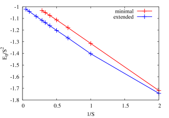
Figure 2: RGM GS energy per site $E_{0}/S^{2}$ in dependence on the inverse spin quantum number $1/S$ (minimal vs. extended version). Note that $E_{0}$ for the extended version naturally coincides with the CCM data of Götze et al. (2011); Götze and Richter (2015).

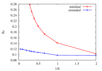
Figure 3: RGM GS static uniform susceptibility $\chi_{0}$ in dependence on the inverse spin quantum number $1/S$ (minimal vs. extended version).

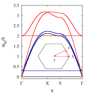
Figure 4: RGM GS results for the dispersion of the magnetic excitations $\omega_{\gamma\mathbf{q}}/S$ ($\gamma=1,2,3$) for $S=1/2$ (red lines) and $S=3$ (blue lines) compared with data of the LSWT (black lines) along a typical path in the first Brillouin zone (see inset). LSWT formulas for $\omega_{\gamma\mathbf{q}}/S$ can be found, e.g., in Chernyshev and Zhitomirsky (2015).

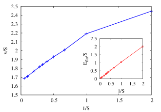
Figure 5: Main: Normalized RGM GS excitation velocity $v(0)/S$ in dependence on the inverse spin quantum number $1/S$. Inset: Position $E_{\rm flat}/S$ of the flat band in dependence on the inverse spin quantum number $1/S$.

We start with the discussion of the RGM results for the GS properties using the minimal as well as the extended (i.e., with CCM input) version of the RGM. In Fig. 2 we show the GS energy $E_{0}/S^{2}$ as a function of the inverse spin quantum number $1/S$. It is obvious that the minimal version leads to significant higher energy values, where for $S=1/2$ the difference is smallest. It is also obvious, that the minimal version does not yield the correct classical large-$S$ limit, $\lim_{S\to\infty}E_{0}/S^{2}=-1$. Thus, we conclude that the minimal version is only applicable for small values of $S$. This conclusion is supported by the data for the static uniform susceptibility $\chi_{0}$ shown in Fig. 3. In what follows (i.e., figures subsequent to Fig. 3), we therefore focus on the discussion of the results obtained by the extended version, i.e., unless stated otherwise, all data presented below belong to the extended version. Now we discuss the excitation spectrum shown in Fig. 4. We mention first, that in linear spin-wave theory (LSWT) $\omega_{\gamma\mathbf{q}}/S$ is independent of $S$, the flat band $\omega_{1}$ is exactly at zero energy and the two dispersive branches, $\omega_{2\mathbf{q}}$ and $\omega_{3\mathbf{q}}$, are degenerate Chernyshev and Zhitomirsky (2015). The RGM provides an improved description of the excitation energies. The flat band is of course also present, but its position $E_{\rm flat}$ depends on $S$, where $E_{\rm flat}/S$ decreases almost linearly with $1/S$ down to $E_{\rm flat}/S=0$ as $S\to\infty$, see inset of Fig. 5. Moreover, the degeneracy of $\omega_{2\mathbf{q}}$ and $\omega_{3\mathbf{q}}$ is lifted and there is a noticeable dependence of the dispersive branches on $S$. In particular, in the extreme quantum case $S=1/2$ the dispersion relations deviate strongly from the LSWT. As increasing $S$ the RGM data approach the LSWT result.

The GS excitation velocity $v$ corresponding to the linear expansion of the lowest branch $\omega_{3\mathbf{q}}$ around the $\Gamma$ point is given by $v^{2}=(\frac{2}{3}S(S+1)+\tilde{\lambda}_{1,0}-4\tilde{\alpha}_{1,0}+\tilde{\alpha}_{1,1}+\tilde{\alpha}_{2,0})$. The LSWT result is $v_{LSWT}=\sqrt{3}S$. Numerical data for $v$ are shown in Fig. 5. While in LSWT $v/S$ is independent of $S$, within the RGM there is a noticeable dependence of $v/S$ on $S$.

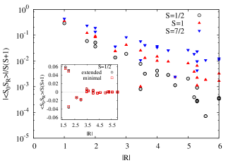
Figure 6: Main: Magnitude of the GS correlation functions $|\langle\hat{\mathbf{S}}_{0}\hat{\mathbf{S}}_{\mathbf{R}}\rangle|/S(S+1)$ within a range of separation $|\mathbf{R}|\leq 6$ for spin quantum numbers $S=1/2,1$ and $7/2$. Inset: Comparison of $\langle\hat{\mathbf{S}}_{0}\hat{\mathbf{S}}_{\mathbf{R}}\rangle/S(S+1)$ of the minimal and extended version of the RGM for $S=1/2$ (nearest-neighbor correlation not included).

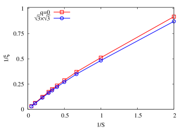
Figure 7: RGM GS correlation lengths corresponding to $q=0$ ($\xi_{\mathbf{Q}_{0}}$) and $\sqrt{3}\times\sqrt{3}$ ($\xi_{\mathbf{Q}_{1}}$) ordering.

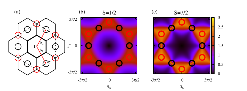
Figure 8: RGM GS structure factor ${\cal S}(\mathbf{q})/S(S+1)$. (a) Brillouin zones: the solid and dashed lines show the first and extended Brillouin zones; the red (black) circles indicate the expected maxima for a classical $\sqrt{3}\times\sqrt{3}$ ($q=0$) state. (b) $S=1/2$, (c) $S=7/2$.

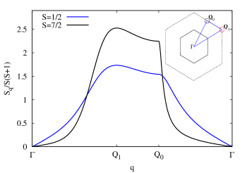
Figure 9: Normalized RGM GS structure factor ${\cal S}(\mathbf{q})/S(S+1)$ along the path $\Gamma\to{\mathbf{Q}_{1}}\to{\mathbf{Q}_{0}}\to\Gamma$ (see inset) for $S=1/2$ and $S=7/2$.

Let us turn to the spin-spin correlation functions $\langle\hat{\mathbf{S}}_{0}\hat{\mathbf{S}}_{\mathbf{R}}\rangle$. In Fig. 6, main panel, we show all non-equivalent GS correlators $\langle\hat{\mathbf{S}}_{0}\hat{\mathbf{S}}_{\mathbf{R}}\rangle/S(S+1)$ up to a separation $R=|\mathbf{R}|=6$ for some selected values of $S$ using a logarithmic scale for $|\langle\hat{\mathbf{S}}_{0}\hat{\mathbf{S}}_{\mathbf{R}}\rangle|/S(S+1)$. In the inset we compare the minimal with the extended version for $S=1/2$ without using a logarithmic scale. Note that the presented data for the minimal version correspond to the results of Bernhard, Canals and Lacroix Bernhard et al. (2002). In accordance with Figs. 2 and 3 for $S=1/2$ the difference between the minimal and the extended version are not tremendous but noticeable. Since for a certain separation $|\mathbf{R}|$ non-equivalent sites exist, more than one data point can appear at one and the same separation $|\mathbf{R}|$. The data suggest that the overall decay of $\ln|\langle\hat{\mathbf{S}}_{0}\hat{\mathbf{S}}_{\mathbf{R}}\rangle/S(S+1)|$ seems to be linear, thus indicating an exponential decay of the correlators. It is also obvious, that the decay is faster the lower the spin quantum number $S$. This observation from Fig. 6 is in agreement with results for the correlation lengths $\xi_{\mathbf{Q}_{0}}$ (corresponding to $q=0$ ordering) and $\xi_{\mathbf{Q}_{1}}$ (corresponding to $\sqrt{3}\times\sqrt{3}$ ordering), shown in Fig. 7 (for the definition of $\xi_{\mathbf{Q}_{0}}$ and $\xi_{\mathbf{Q}_{1}}$ see Sec. II.1). In the extreme quantum spin-half case the correlation lengths are of the order of one lattice spacing as expected in a spin liquid. That is in agreement with known results, e.g., obtained by large-scale density-matrix renormalization-group (DMRG) studies Kolley et al. (2015). The RGM data then indicate a power-law increase of both, $\xi_{\mathbf{Q}_{0}}$ and $\xi_{\mathbf{Q}_{1}}$, with increasing $S$, see Fig. 7. We find $\xi_{\mathbf{Q}_{1}}>\xi_{\mathbf{Q}_{0}}$ for all $S$, but the difference of both correlation lengths is small.

Now we discuss the GS static magnetic structure factor ${\cal S}(\mathbf{q})$. In Fig. 8 we show an intensity plot of ${\cal S}(\mathbf{q})/S(S+1)$ using an extended Brillouin zone, see panel (a) and cf. also Kolley et al. (2015). For $S=1/2$ we find the typical pattern Läuchli and Lhuillier (2009); Depenbrock et al. (2012); Kolley et al. (2015), i.e., the intensity is concentrated along the edge of the extended Brillouin zone, where ${\cal S}(\mathbf{q})$ remains small even at the magnetic $\mathbf{q}$-vectors $\mathbf{Q}_{0}$ and $\mathbf{Q}_{1}$ related to the $q=0$ and $\sqrt{3}\times\sqrt{3}$ states. This smooth shape of ${\cal S}(\mathbf{q})$ is related to the fast decay of the spin-spin correlations, see Fig. 6. As increasing $S$ the structure factor develops a more pronounced shape, and pinch points, typical for the classical KHAF Zhitomirsky (2008), emerge between triangular shaped areas of large intensity, see Fig. 8c. This observation is also obvious from Fig. 9, where we show the structure factor along a prominent path in the extended Brillouin zone. As indicated by Figs. 8 and 9, we find that for all values of $S$ the relation ${\cal S}(\mathbf{Q}_{1})>{\cal S}(\mathbf{Q}_{0})$ holds. Together with the data for the correlation lengths $\xi_{\mathbf{Q}_{0}}$ and $\xi_{\mathbf{Q}_{1}}$ (Fig. 7) we may conclude that $\sqrt{3}\times\sqrt{3}$ SRO is favored in agreement with previous investigations Chubukov (1992); Sachdev (1992); Henley and Chan (1995); Götze et al. (2011); Chernyshev and Zhitomirsky (2014).

From the static GS properties reported above we conclude that, although the magnetic SRO with $\sqrt{3}\times\sqrt{3}$ symmetry becomes more and more pronounced with increasing $S$, within the RGM approach no magnetic LRO for the spin-$S$ KHAF is found. We may compare this finding with known GS results obtained by other methods. Note, however, that for $S>1$ data to compare with are extremely rare. We mention first that within the LSWT the quantum correction of the sublattice magnetization always diverges due to the zero-energy flat band, see, e.g., Chernyshev and Zhitomirsky (2014). As briefly discussed in the introduction, more sophisticated GS methods such as the CCM and the DMRG yield evidence that for $S=1$ semiclassical magnetic LRO is also lacking Götze et al. (2011); Götze and Richter (2015); Changlani and Läuchli (2015); Liu et al. (2015); Picot and Poilblanc (2015); Nishimoto and Nakamura (2015). On the other hand, recent results obtained by CCM, tensor network approaches, and series expansion indicate weak GS $\sqrt{3}\times\sqrt{3}$ LRO for $S=3/2$ Götze et al. (2011); Götze and Richter (2015); Oitmaa and Singh (2016); Liu et al. (2016). Previous experience in applying the RGM on frustrated quantum antiferromagnets, see, e.g., Barabanov and Beresovsky (1994); Siurakshina et al. (2001); Schmalfuß et al. (2004); Härtel et al. (2013); Mikheyenkov et al. (2013) and references therein, indicate, however, that the implementation of rotational invariance by setting $\langle\hat{S}^{z}_{i}\rangle=0$ in the equations of motions may overestimate the tendency to melt semiclassical GS magnetic LRO in RGM calculations.

III.2 Finite-temperature properties

In what follows, as a rule we will present the temperature dependence of physical quantities using a normalized temperature $T/S(S+1)$. This choice ensures a spin-independent behavior of the physical quantities at large temperatures Schmidt et al. (2011). Moreover, we mention again that (unless stated otherwise) we present RGM data for the extended version using CCM input (see above).

III.2.1 Spin-spin correlation functions, specific heat and uniform susceptibility

We start with the discussion of the temperature dependence of short-range spin-spin correlation functions $\langle\hat{\mathbf{S}}_{0}\hat{\mathbf{S}}_{\mathbf{R}}\rangle$. We show the absolute values in Fig. 10, main panel, for $S=1/2$, $1$, and $7/2$. (Note that the NN correlation is antiferromagnetic, whereas the NNN and NNNN correlation functions are ferromagnetic.) We find that there is a low-temperature region $T/S(S+1)\lesssim 0.1$ where the presented correlation functions are almost temperature independent. This region is largest for the extreme quantum case $S=1/2$. It is also obvious that for $T/S(S+1)<1$ the magnetic SRO becomes more pronounced as increasing $S$ (cf. also Fig. 6). On the other hand, for $T/S(S+1)>1$ the curves for various $S$ practically coincide. In the inset of Fig. 10 we compare the two versions of the RGM (minimal and extended) as well as the HTE series for $S=1/2$. Obviously, both versions of the RGM agree well with each other. Note, however, that this statement does not hold for larger values of $S$, cf. the discussion in Sec. III.1. The HTE approach for correlation functions is also in good agreement with the RGM data down to $T\sim 0.4$.

Now we turn to the specific heat. For the extreme quantum case $S=1/2$ various methods provide indications for an additional low-temperature peak at about $T=0.1$ Elstner and Young (1994); Nakamura and Miyashita (1995); Tomczak and Richter (1996); Sindzingre et al. (2000); Misguich and Bernu (2005); Rigol et al. (2007); Munehisa (2014); Shimokawa and Kawamura (2016) due to a set of low-lying singlet states. However, instead of a true maximum a shoulder-like hump may characterize the low-$T$ profile of $C(T)$ Misguich and Bernu (2005); Chen et al. (2017). It is an open question whether for $S>1/2$ such a feature is still present. Our RGM approach does not show any unconventional feature in the temperature profile of the specific heat at low $T$ for $S=1/2$ and $S=1$, cf. Fig. 11. For $S>1$ a weakly pronounced shoulder-like hump emerges (see the inset of Fig. 11). We argue, that our RGM approach is not able to detect the subtle role of low-lying excitations relevant for the low-temperature physics of the KHAF in the extreme quantum limit of small spin $S$. On the other hand, in the limit of large $S$ the RGM data seem to approach the classical Monte-Carlo data Chalker et al. (1992); García-Adeva and Huber (2001) reasonably well.

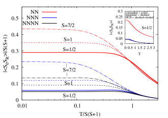
Figure 10: Main panel: Magnitude of the normalized spin-spin correlation functions $|\langle\hat{\mathbf{S}}_{0}\hat{\mathbf{S}}_{\mathbf{R}}\rangle|/S(S+1)$ as a function of the normalized temperature $T/S(S+1)$ (logarithmic scale) for spin quantum numbers $S=1/2,1$, and $7/2$ (NN – nearest neighbors; NNN – next-nearest neighbors; NNNN – next-next-nearest neighbors along two $J_{1}$ bonds). Inset: Magnitude of the spin-spin correlation functions $|\langle\hat{\mathbf{S}}_{0}\hat{\mathbf{S}}_{\mathbf{R}}\rangle|$ for $S=1/2$ as a function of the temperature $T$ (linear scale): Comparison of the extended (solid) and minimal (dashed) versions of the RGM as well as the 11th-order HTE with subsequent Padé (dashed-dotted).

The temperature dependence of the static uniform susceptibility $\chi_{0}$ for spin quantum numbers $S=1/2,1,\ldots,7/2$ is shown in Fig. 12. Similar as for the specific heat there is a well-pronounced tendency to shift the typical maximum in $\chi_{0}(T)$ towards lower values of $T/S(S+1)$ and to enlarge the height of the maximum as increasing $S$. Again, in the limit of large $S$ the RGM data seem to approach the classical Monte-Carlo data Reimers and Berlinsky (1993); García-Adeva and Huber (2001) reasonably well. The fact that $\chi_{0}(T=0)$ is finite, cf. also Fig. 3, is in favor of a vanishing gap to magnetic excitations. There is an ongoing controversial discussion of the gap issue for the $S=1/2$ KHAF Yan et al. (2011); Depenbrock et al. (2012); Läuchli et al. (2011, 2016); Iqbal et al. (2011, 2013); Liao et al. (2017). However, we do not claim, that our approach is accurate enough at low temperatures in the quantum limit of small $S$ to provide reliable statements on the very existence of an excitation gap.

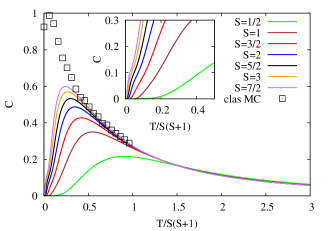
Figure 11: Main: Specific heat $C$ for various values of the spin quantum number $S$ as a function of the normalized temperature $T/S(S+1)$. The Monte-Carlo data for the classical limit are taken from Reimers and Berlinsky (1993); García-Adeva and Huber (2001). Inset: Low-temperature behavior of $C$ using an enlarged scale.

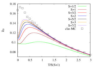
Figure 12: Uniform static susceptibility $\chi_{0}$ for various values of the spin $S$ as a function of the normalized temperature $T/S(S+1)$. The Monte-Carlo data for the classical limit are taken from García-Adeva and Huber (2001).

III.2.2 Structure factor and correlation lengths

To get more insight in the magnetic ordering of the KHAF at finite temperatures we investigate the structure factor and the correlation lengths. Some information on magnetic SRO has already been provided in Fig. 10. First we show in Fig. 13 an intensity plot of the static structure factor ${\cal S}(\mathbf{q})/S(S+1)$ for $S=1/2$ and $S=3$ for $T/S(S+1)=1.3$ and compare RGM and HTE. The overall impression is that the RGM and HTE approaches yield very similar intensity plots of ${\cal S}(\mathbf{q})/S(S+1)$. The characteristic hexagonal bow-tie pattern (i.e., the intensity is concentrated along the edge of the extended Brillouin zone), which was found at $T=0$, cf. Fig. 8, is still present at $T/S(S+1)=1.3$.

Next we show in Fig. 14 the static structure factor ${\cal S}(\mathbf{q})/S(S+1)$ along the path $\Gamma\to{\mathbf{Q}_{1}}\to{\mathbf{Q}_{0}}\to\Gamma$ for $S=1/2$ and $S=7/2$ for $T/S(S+1)=1.5$ (RGM and HTE) and $T=0$ (only RGM, see also Fig. 9). Obviously, the temperature $T/S(S+1)=1.5$ is already large enough, such that all four curves are very close to each other. Although, the weakening of magnetic ordering by thermal fluctuations is evident, the overall shape of the finite-temperature curves is similar to the GS curves, especially the maxima at ${\mathbf{Q}_{1}}$ ($\sqrt{3}\times\sqrt{3}$ state) and at ${\mathbf{Q}_{0}}$ ($q=0$ state) are still present, and ${\cal S}(\mathbf{Q}_{1})>{\cal S}(\mathbf{Q}_{0})$.

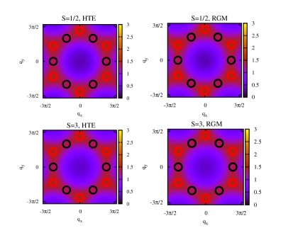
Figure 13: Intensity plot of the normalized structure factor ${\cal S}(\mathbf{q})/S(S+1)$ within the first and extended Brillouin zones [cf. Fig. 8(a)] for $S=1/2$ and $S=3$ at $T/S(S+1)=1.3$ (left: 9th order HTE, right: RGM). The red (black) circles indicate the expected maxima for a classical $\sqrt{3}\times\sqrt{3}$ ($q=0$) state.

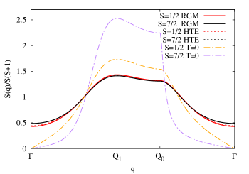
Figure 14: RGM and HTE data for the normalized structure factor ${\cal S}(\mathbf{q})/S(S+1)$ along the path $\Gamma\to{\mathbf{Q}_{1}}\to{\mathbf{Q}_{0}}\to\Gamma$ for $S=1/2$ and $S=7/2$ at $T/S(S+1)=1.5$. For comparison we also present RGM data for $T=0$ (dashed-dotted lines).

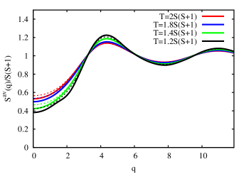
Figure 15: Normalized powder-averaged structure factor ${\cal S}^{\rm av}(|\mathbf{q}|)/S(S+1)$ for spin $S=1/2$ (solid lines) and $S=7/2$ (dashed lines) using HTE of 9th order.

In experiments, often neutron scattering on powder samples are performed, see, e.g. de Vries et al. (2009). Hence, we also present the powder-averaged structure factor ${\cal S}^{\rm av}(|\mathbf{q}|)/S(S+1)$, i.e., we integrate over all points at equal $q=|\mathbf{q}|$. We show HTE data for ${\cal S}^{\rm av}(|\mathbf{q}|)/S(S+1)$ for $S=1/2$ and $S=7/2$ at various temperatures in Fig. 15. The first broad maximum at $|\mathbf{q}|\sim 4.36$ corresponds to short-ranged antiferromagnetic correlations and its position is in good agreement with experiments on Herbertsmithite de Vries et al. (2009). (Note that the separation of NN copper ions in Herbertsmithite is $a=3.4$Å, here we use $a=1$.) While the influence of $T$ on the height of the maxima in $S^{\rm av}(|\mathbf{q}|)$ is recognizable, the position of the maxima is almost independent of $T$. Thus, from Fig. 15 and Fig. 14 one can conclude that the type of magnetic SRO found at pretty high temperatures $T/S(S+1)>1$ indicate a possible magnetic ordering at low temperatures.

Last but not least we discuss the temperature dependence of the structure factors at the magnetic wave vectors $\mathbf{Q}_{0}$ ($q=0$ state) and $\mathbf{Q}_{1}$ ($\sqrt{3}\times\sqrt{3}$ state) and of the corresponding correlation lengths $\xi_{\mathbf{Q}_{0}}$ and $\xi_{\mathbf{Q}_{1}}$, see Figs. 16 and 17. First we note that the $\sqrt{3}\times\sqrt{3}$ SRO is more pronounced than the $q=0$ SRO for all temperatures $T\geq 0$, i.e., ${\cal S}(\mathbf{Q}_{1})|_{T}>{\cal S}(\mathbf{Q}_{0})|_{T}$ and $\xi_{\mathbf{Q}_{1}}(T)>\xi_{\mathbf{Q}_{0}}(T)$ (cf. also Figs. 7 and 9 for the GS). As increasing $S$ the SRO becomes more distinct. Only at temperatures $T/S(S+1)\gtrsim 1$ the curves for different $S$ collapse to one universal curve, cf. Lohmann et al. (2014). At low temperatures $T<T^{*}$ we find a plateau-like behavior in the correlation lengths and the structure factors, $\xi_{\mathbf{Q}_{i}}|_{T<T^{*}}\approx\xi_{\mathbf{Q}_{i}}|_{T=0}$ and ${\cal S}(\mathbf{Q}_{i})|_{T<T^{*}}\approx{\cal S}(\mathbf{Q}_{i})|_{T=0}$. The region of almost constant correlation lengths and structure factors is largest for $S=1/2$ and it shrinks noticeably as increasing $S$ approaching zero in the classical limit ($\lim_{S\to\infty}T^{*}/S(S+1)=0$). To define a reasonable estimate of $T^{*}$ we chose that value of $T$, where correlation lengths and the structure factors reach $p=99\%$ of its GS values. The corresponding data are shown in Fig. 18. We mention that for the correlation lengths the relation $T^{*}=a/S(S+1)$ describes the plotted behavior accurately, where $a=0.2$ for $p=99\%$. (Note that the prefactor $a$ increases only slightly to $a=0.28$ as changing $p$ to $p=95\%$.) We may argue that below $T^{*}$ the quantum fluctuations are more important than thermal fluctuations.

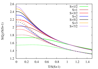
Figure 16: RGM data for the normalized structure factor ${\cal S}(\mathbf{Q}_{i})/S(S+1)$ at the magnetic wave vector $\mathbf{Q}_{i}$ (dashed - $\mathbf{Q}_{0}$; solid - $\mathbf{Q}_{1}$) for various values of the spin $S$ as a function of the normalized temperature $T/S(S+1)$.

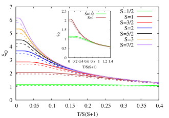
Figure 17: Main: RGM data for the correlation length $\xi_{\mathbf{Q}_{i}}$ (dashed - $\mathbf{Q}_{0}$; solid - $\mathbf{Q}_{1}$) for various values of the spin $S$ as a function of the normalized temperature $T/S(S+1)$. Inset: Correlation lengths $\xi_{\mathbf{Q}_{i}}$ (dashed - $\mathbf{Q}_{0}$; solid - $\mathbf{Q}_{1}$) for $S=1/2$ and $S=1$ using an enlarged y-axis.

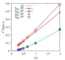
Figure 18: RGM data for the temperature region $T^{*}/S(S+1)$ of almost almost constant ($p=99\%$, see text) correlation lengths and structure factors as a function of $1/S$. The green line corresponds the fit function $f(S)=0.2/S(S+1)$.

IV Summary

We use two methods to discuss the thermodynamic properties of the kagome Heisenberg antiferromagnet with arbitrary spin $S$, namely the rotational invariant Green’s function method (RGM) and the high-temperature expansion (HTE). Within the RGM we consider GS as well as finite-temperature properties, whereas the HTE is restricted to $T/S(S+1)\gtrsim 1$. Within the RGM approach the model does not exhibit magnetic LRO for all values of $S$. In the extreme quantum case $S=1/2$ the zero-temperature correlation length $\xi(T=0)$ is only of the order of the nearest-neighbor separation. As increasing $S$ the correlation length $\xi(T=0)$ grows according to a power-law in $1/S$. We found that the so-called $\sqrt{3}\times\sqrt{3}$ SRO is favored versus the $q=0$ SRO for all values of $S$. It is worth mentioning that other methods specifically designed for the GS Götze et al. (2011); Götze and Richter (2015); Oitmaa and Singh (2016); Liu et al. (2016) indicate that GS LRO may appear for $S\geq 3/2$. As known from previous studies the rotational invariant decoupling in the RGM scheme may overestimate the tendency to suppress magnetic order, cf. Barabanov and Beresovsky (1994); Siurakshina et al. (2001); Schmalfuß et al. (2004); Härtel et al. (2013); Mikheyenkov et al. (2013) and references therein.

As typical for two-dimensional Heisenberg antiferromagnets, the specific heat and the uniform susceptibility exhibit a maximum related to the size of the exchange coupling $J$. For both quantities, with growing $S$ this maximum moves towards lower values of $T/S(S+1)$ and its height increases. In the limit of large $S$ the RGM data approach the classical curves.

The structure factor ${\cal S}(\mathbf{q})$ shows two maxima at magnetic wave vectors $\mathbf{q}={\mathbf{Q}_{i}},i=0,1$, corresponding to the $q=0$ and $\sqrt{3}\times\sqrt{3}$ state, where ${\cal S}(\mathbf{Q}_{1})>{\cal S}(\mathbf{Q}_{0})$ holds for all values of $S$ and all temperatures $T\geq 0$. In a finite low-temperature region $T<T^{*}\approx a/S(S+1),a\approx 0.2$, the magnetic SRO is quite stable against thermal fluctuations, i.e., the correlation lengths and the structure factors ${\cal S}(\mathbf{Q}_{1})$ and ${\cal S}(\mathbf{Q}_{0})$ are almost independent of $T$. The powder-averaged structure factor ${\cal S}(|\mathbf{q}|)$ exhibits a broad maximum related to short-ranged antiferromagnetic correlations and its position is in good agreement with experiments on powder samples of Herbertsmithite de Vries et al. (2009).

References

- Zeng and Elser (1990) C. Zeng and V. Elser, “Numerical studies of antiferromagnetism on a kagomé net,” Phys. Rev. B 42, 8436–8444 (1990).
- Chalker et al. (1992) J. T. Chalker, P. C. W. Holdsworth, and E. F. Shender, “Hidden order in a frustrated system: Properties of the Heisenberg kagomé antiferromagnet,” Phys. Rev. Lett. 68, 855–858 (1992).
- Harris et al. (1992) A. B. Harris, C. Kallin, and A. J. Berlinsky, “Possible Néel orderings of the kagomé antiferromagnet,” Phys. Rev. B 45, 2899–2919 (1992).
- Singh and Huse (1992) R. R. P. Singh and D. A. Huse, “Three-sublattice order in triangular- and kagomé-lattice spin-half antiferromagnets,” Phys. Rev. Lett. 68, 1766–1769 (1992).
- Reimers and Berlinsky (1993) J. N. Reimers and A. J. Berlinsky, “Order by disorder in the classical Heisenberg kagomé antiferromagnet,” Phys. Rev. B 48, 9539–9554 (1993).
- Elstner et al. (1993) N. Elstner, R. R. P. Singh, and A. P. Young, “Finite temperature properties of the spin-1/2 Heisenberg antiferromagnet on the triangular lattice,” Phys. Rev. Lett. 71, 1629–1632 (1993).
- Elstner and Young (1994) N. Elstner and A. P. Young, “Spin-1/2 Heisenberg antiferromagnet on the kagome lattice: High-temperature expansion and exact-diagonalization studies,” Phys. Rev. B 50, 6871–6876 (1994).
- Henley and Chan (1995) C. L. Henley and E. P. Chan, “Ground state selection in a kagomé antiferromagnet,” J. Magn. Magn. Mater. 140-144, 1693–1694 (1995).
- Nakamura and Miyashita (1995) T. Nakamura and S. Miyashita, “Thermodynamic properties of the quantum Heisenberg antiferromagnet on the kagomé lattice,” Phys. Rev. B 52, 9174–9177 (1995).
- Tomczak and Richter (1996) P. Tomczak and J. Richter, “Thermodynamical properties of the Heisenberg antiferromagnet on the kagomé lattice,” Physical Review B 54, 9004 (1996).
- Waldtmann et al. (1998) C. Waldtmann, H.-U. Everts, B. Bernu, C. Lhuillier, P. Sindzingre, P. Lecheminant, and L. Pierre, “First excitations of the spin 1/2 Heisenberg antiferromagnet on the kagomé lattice,” EPJB 2, 501–507 (1998).
- Yu and Feng (2000) W. Yu and S. Feng, “Spin-liquid state for two-dimensional Heisenberg antiferromagnets on a kagomé lattice,” EPJB 13, 265–269 (2000).
- Sindzingre et al. (2000) P. Sindzingre, G. Misguich, C. Lhuillier, B. Bernu, L. Pierce, C. Waldtmann, and H. U. Everts, “Magnetothermodynamics of the spin-1/2 kagome antiferromagnet,” Phys. Rev. Lett. 84, 2953–2956 (2000).
- García-Adeva and Huber (2001) A. J. García-Adeva and D. L. Huber, “Classical generalized constant coupling model for geometrically frustrated antiferromagnets,” Phys. Rev. B 63, 140404 (2001).
- Bernhard et al. (2002) B. H. Bernhard, B. Canals, and C. Lacroix, “Green’s function approach to the magnetic properties of the kagomé antiferromagnet,” Phys. Rev. B 66, 104424 (2002).
- Schmalfuß et al. (2004) D. Schmalfuß, J. Richter, and D. Ihle, “Absence of long-range order in a spin-half Heisenberg antiferromagnet on the stacked kagomé lattice,” Phys. Rev. B 70, 184412 (2004).
- Misguich and Bernu (2005) G. Misguich and B. Bernu, “Specific heat of the Heisenberg model on the kagome lattice: High-temperature series expansion analysis,” Phys. Rev. B 71, 014417 (2005).
- Singh and Huse (2007) R. R. P. Singh and D. A. Huse, “Ground state of the spin-1/2 kagome-lattice Heisenberg antiferromagnet,” Phys. Rev. B 76, 180407 (2007).
- Li et al. (2007) P. Li, H. Su, and S.-Q. Shen, “Kagome antiferromagnet: A schwinger-boson mean-field theory study,” Phys. Rev. B 76, 174406 (2007).
- Rigol et al. (2007) Marcos Rigol, Tyler Bryant, and Rajiv R. P. Singh, “Numerical linked-cluster algorithms. I. spin systems on square, triangular, and kagome lattices,” Physical Review E 75, 061118 (2007).
- Zhitomirsky (2008) M. E. Zhitomirsky, “Octupolar ordering of classical kagome antiferromagnets in two and three dimensions,” Phys. Rev. B 78, 094423 (2008).
- Jiang et al. (2008) H. C. Jiang, Z. Y. Weng, and D. N. Sheng, “Density matrix renormalization group numerical study of the kagome antiferromagnet,” Phys. Rev. Lett. 101, 117203 (2008).
- Läuchli and Lhuillier (2009) A. M. Läuchli and C. Lhuillier, “Dynamical correlations of the kagome S = 1/2 Heisenberg quantum antiferromagnet,” ArXiv e-prints (2009), arXiv:0901.1065 [cond-mat.str-el] .
- Evenbly and Vidal (2010) G. Evenbly and G. Vidal, “Frustrated antiferromagnets with entanglement renormalization: Ground state of the spin-1/2 Heisenberg model on a kagome lattice,” Phys. Rev. Lett. 104, 187203 (2010).
- Götze et al. (2011) O. Götze, D. J. J. Farnell, R. F. Bishop, P. H. Y. Li, and J. Richter, “Heisenberg antiferromagnet on the kagome lattice with arbitrary spin: A higher-order coupled cluster treatment,” Phys. Rev. B 84, 224428 (2011).
- Nakano and Sakai (2011) H. Nakano and T. Sakai, “Numerical-diagonalization study of spin gap issue of the kagome lattice Heisenberg antiferromagnet,” J. Phys. Soc. Jpn. 80, 053704 (2011).
- Iqbal et al. (2011) Y. Iqbal, F. Becca, and D. Poilblanc, “Projected wave function study of z2 spin liquids on the kagome lattice for the spin-1/2 quantum Heisenberg antiferromagnet,” Phys. Rev. B 84, 020407 (2011).
- Yan et al. (2011) S. Yan, D. A. Huse, and S. R. White, “Spin-liquid ground state of the s = 1/2 Kagome Heisenberg antiferromagnet,” Science 332, 1173–1176 (2011).
- Läuchli et al. (2011) A. M. Läuchli, J. Sudan, and E. S. Sørensen, “Ground-state energy and spin gap of spin-1/2 kagomé-Heisenberg antiferromagnetic clusters: Large-scale exact diagonalization results,” Phys. Rev. B 83, 212401 (2011).
- Depenbrock et al. (2012) S. Depenbrock, I. P. McCulloch, and U. Schollwöck, “Nature of the spin-liquid ground state of the s = 1/2 Heisenberg model on the kagome lattice,” Phys. Rev. Lett. 109, 067201 (2012).
- Rousochatzakis et al. (2013) I. Rousochatzakis, R. Moessner, and J. v. d. Brink, “Frustrated magnetism and resonating valence bond physics in two-dimensional kagome-like magnets,” Phys. Rev. B 88, 195109 (2013).
- Iqbal et al. (2013) Yasir Iqbal, Federico Becca, Sandro Sorella, and Didier Poilblanc, “Gapless spin-liquid phase in the kagome spin- Heisenberg antiferromagnet,” Phys. Rev. B 87, 060405 (2013).
- Rousochatzakis et al. (2014) I. Rousochatzakis, Y. Wan, O. Tchernyshyov, and F. Mila, “Quantum dimer model for the spin-1/2 kagome Z2 spin liquid,” Phys. Rev. B 90, 100406 (2014).
- Xie et al. (2014) Z. Y. Xie, J. Chen, J. F. Yu, X. Kong, B. Normand, and T. Xiang, “Tensor renormalization of quantum many-body systems using projected entangled simplex states,” Phys. Rev. X 4, 011025 (2014).
- Lohmann et al. (2014) A. Lohmann, H.-J. Schmidt, and J. Richter, “Tenth-order high-temperature expansion for the susceptibility and the specific heat of spin-s Heisenberg models with arbitrary exchange patterns: Application to pyrochlore and kagome magnets,” Phys. Rev. B 89, 014415 (2014).
- Munehisa (2014) T. Munehisa, “An improved finite temperature lanczos method and its application to the spin-1/2 Heisenberg model on the kagome lattice,” World Journal of Condensed Matter Physics 4, 134–140 (2014).
- Kolley et al. (2015) F. Kolley, S. Depenbrock, I. P. McCulloch, U. Schollwöck, and V. Alba, “Phase diagram of the - Heisenberg model on the kagome lattice,” Phys. Rev. B 91, 104418 (2015).
- Götze and Richter (2015) O. Götze and J. Richter, “Ground-state phase diagram of the XXZ spin-s kagome antiferromagnet: A coupled-cluster study,” Phys. Rev. B 91, 104402 (2015).
- Changlani and Läuchli (2015) H. J. Changlani and A. M. Läuchli, “Trimerized ground state of the spin-1 Heisenberg antiferromagnet on the kagome lattice,” Phys. Rev. B 91, 100407 (2015).
- Liu et al. (2015) T. Liu, W. Li, A. Weichselbaum, J. v. Delft, and G. Su, “Simplex valence-bond crystal in the spin-1 kagome Heisenberg antiferromagnet,” Phys. Rev. B 91, 060403 (2015).
- Picot and Poilblanc (2015) T. Picot and D. Poilblanc, “Nematic and supernematic phases in kagome quantum antiferromagnets under the influence of a magnetic field,” Phys. Rev. B 91, 064415 (2015).
- Nishimoto and Nakamura (2015) S. Nishimoto and M. Nakamura, “Non-symmetry-breaking ground state of the S=1 Heisenberg model on the kagome lattice,” Phys. Rev. B 92, 140412 (2015).
- Liu et al. (2016) T. Liu, W. Li, and G. Su, “Spin-ordered ground state and thermodynamic behaviors of the spin- kagome Heisenberg antiferromagnet,” Phys. Rev. E 94, 032114 (2016).
- Shimokawa and Kawamura (2016) T. Shimokawa and H. Kawamura, “Finite-temperature crossover phenomenon in the s=1/2 antiferromagnetic Heisenberg model on the kagome lattice,” J. Phys. Soc. Jpn. 85, 113702 (2016).
- Oitmaa and Singh (2016) J. Oitmaa and R. R. P. Singh, “Competing orders in spin-1 and spin-3/2 XXZ kagome antiferromagnets: A series expansion study,” Phys. Rev. B 93, 014424 (2016).
- Götze and Richter (2016) O. Götze and J. Richter, “The route to magnetic order in the spin-1/2 kagome Heisenberg antiferromagnet: The role of interlayer coupling,” EPL 114, 67004 (2016).
- Läuchli et al. (2016) A. M. Läuchli, J. Sudan, and R. Moessner, “The kagome S = 1/2 Heisenberg antiferromagnet revisited,” ArXiv e-prints (2016), arXiv:1611.06990 [cond-mat.str-el] .
- He et al. (2017) Y.C. He, M. P. Zaletel, M.Oshikawa, and F. Pollmann, “Signatures of Dirac cones in a dmrg study of the kagome Heisenberg model,” Phys. Rev. X 7, 031020 (2017).
- Liao et al. (2017) H. J. Liao, Z. Y. Xie, J. Chen, Z. Y. Liu, H. D. Xie, R. Z. Huang, B. Normand, and T. Xiang, “Gapless spin-liquid ground state in the s=1/2 kagome antiferromagnet,” Phys. Rev. Lett. 118, 137202 (2017).
- P. and Singh (2017) N. E. Sherman P. and R. R. P. Singh, “Structure factors of the kagome-lattice Heisenberg antiferromagnets at finite temperatures,” ArXiv e-prints (2017), arXiv:1711.053375 [cond-mat.str-el] .
- Chen et al. (2017) X. Chen, S.-J. Ran, T. Liu, C. Peng, Y.-Z. Huang, and G. Su, “Finite-temperature phase diagram and algebraic paramagnetic liquid in the spin-1/2 kagome Heisenberg antiferromagnet,” ArXiv e-prints (2017), arXiv:1711.01001 [cond-mat.str-el] .
- Villain et al. (1980) J. Villain, R. Bidaux, J.-P. Carton, and R. Conte, “Order as an effect of disorder,” J. Phys. 41, 1263–1272 (1980).
- Shender (1982) E. F. Shender, “Antiferromagnetic garnets with fluctuationally interacting sublattices,” JETP 56, 178–184 (1982).
- Mendels et al. (2007) P. Mendels, F. Bert, M. A. de Vries, A. Olariu, A. Harrison, F. Duc, J. C. Trombe, J. S. Lord, A. Amato, and C. Baines, “Quantum magnetism in the paratacamite family: Towards an ideal kagomé lattice,” Phys. Rev. Lett. 98, 077204 (2007).
- Helton et al. (2007) J. S. Helton, K. Matan, M. P. Shores, E. A. Nytko, B. M. Bartlett, Y. Yoshida, Y. Takano, A. Suslov, Y. Qiu, J.-H. Chung, D. G. Nocera, and Y. S. Lee, “Spin Dynamics of the Spin-1/2 Kagome Lattice AntiferromagnetZnCu3(OH)6Cl2,” Phys. Rev. Lett. 98, 107204 (2007).
- Hiroi et al. (2009) Z. Hiroi, H. Yoshida, Y. Okamoto, and M. Takigawa, “Spin-1/2 kagome compounds: Volborthite vs herbertsmithite,” J. Phys.: Conf. Ser. 145, 012002 (2009).
- de Vries et al. (2009) M. A. de Vries, J. R. Stewart, P. P. Deen, J. O. Piatek, G. J. Nilsen, H. M. Rønnow, and A. Harrison, “Scale-free antiferromagnetic fluctuations in the s=1/2 kagome antiferromagnet herbertsmithite,” Phys. Rev. Lett. 103, 237201 (2009).
- Wulferding et al. (2010) D. Wulferding, P. Lemmens, P. Scheib, J. Röder, P. Mendels, S. Chu, T. Han, and Y. S. Lee, “Interplay of thermal and quantum spin fluctuations in the kagome lattice compound herbertsmithite,” Phys. Rev. B 82, 144412 (2010).
- Han et al. (2012) T.-H. Han, J. S. Helton, S. Chu, D. G. Nocera, J. A. Rodriguez-Rivera, C. Broholm, and Y. S. Lee, “Fractionalized excitations in the spin-liquid state of a kagome-lattice antiferromagnet,” Nature 492, 406–410 (2012).
- Fåk et al. (2007) B. Fåk, F. C. Coomer, A. Harrison, D. Visser, and M. E. Zhitomirsky, “Spin-liquid behavior in a kagomé antiferromagnet: Deuteronium jarosite,” EPL 81, 17006 (2007).
- Okubo et al. (2017) S. Okubo, R. Nakata, S. Ikeda, N. Takahashi, T. Sakurai, W.-M. Zhang, H. Ohta, T. Shimokawa, T. Sakai, K. Okuta, S. Hara, and H. Sato, “Dzyaloshinsky-Moriya interaction and the ground state in s = 3/2 perfect kagome lattice antiferromagnet KCr3(OH)6(SO4)2 (cr-jarosite) studied by x-band and high-frequency ESR,” J. Phys. Soc. Jpn. 86, 024703 (2017).
- Sachdev (1992) S. Sachdev, “Kagome´- and triangular-lattice Heisenberg antiferromagnets: Ordering from quantum fluctuations and quantum-disordered ground states with unconfined bosonic spinons,” Phys. Rev. B 45, 12377–12396 (1992).
- Chubukov (1992) A. Chubukov, “Order from disorder in a kagomé antiferromagnet,” Phys. Rev. Lett. 69, 832–835 (1992).
- Chernyshev and Zhitomirsky (2014) A. L. Chernyshev and M. E. Zhitomirsky, “Quantum selection of order in an antiferromagnet on a kagome lattice,” Phys. Rev. Lett. 113, 237202 (2014).
- Chernyshev and Zhitomirsky (2015) A. L. Chernyshev and M. E. Zhitomirsky, “Order and excitations in large-s kagome-lattice antiferromagnets,” Phys. Rev. B 92, 144415 (2015).
- Gasser et al. (2001) W. Gasser, E. Heiner, and K. Elk, Greensche Funktionen in Festkörper- und Vielteilchenphysik (Wiley-Blackwell, 2001).
- Nolting and Ramakanth (2009) W. Nolting and A. Ramakanth, Quantum Theory of Magnetism (Springer Science & Business Media, 2009).
- Fröbrich and Kuntz (2006) P. Fröbrich and P. J. Kuntz, “Many-body green’s function theory of Heisenberg films,” Phys. Rep. 432, 223–304 (2006).
- Rosner et al. (2003) H. Rosner, R. R. P. Singh, W. H. Zheng, J. Oitmaa, and W. E. Pickett, “High-temperature expansions for the Heisenberg models: Applications to ab initio calculated models for and ,” Phys. Rev. B 67, 014416 (2003).
- Singh and Oitmaa (2012) R. R. P. Singh and J. Oitmaa, “High-temperature series expansion study of the Heisenberg antiferromagnet on the hyperkagome lattice: Comparison with na4ir3o8,” Phys. Rev. B 85, 104406 (2012).
- Bernu et al. (2013) B. Bernu, C. Lhuillier, E. Kermarrec, F. Bert, P. Mendels, R. H. Colman, and A. S. Wills, “Exchange energies of kapellasite from high-temperature series analysis of the kagome lattice -Heisenberg model,” Phys. Rev. B 87, 155107 (2013).
- Oitmaa et al. (2006) J. Oitmaa, C. Hamer, and W. Zheng, Series Expansion Methods for Strongly Interacting Lattice Models (Cambridge University Press, 2006).
- Bernu and Misguich (2001) B. Bernu and G. Misguich, “Specific heat and high-temperature series of lattice models: Interpolation scheme and examples on quantum spin systems in one and two dimensions,” Phys. Rev. B 63, 134409 (2001).
- Bernu and Lhuillier (2015) B. Bernu and C. Lhuillier, “Spin susceptibility of quantum magnets from high to low temperatures,” Phys. Rev. Lett. 114, 057201 (2015).
- Schmidt et al. (2011) H.-J. Schmidt, A. Lohmann, and J. Richter, “Eighth-order high-temperature expansion for general Heisenberg hamiltonians,” Phys. Rev. B 84, 104443 (2011).
- Richter et al. (2015) J. Richter, P. Müller, A. Lohmann, and H.-J. Schmidt, “High-temperature expansion for frustrated magnets: Application to the - model on the BCC lattice,” Phys. Procedia 75, 813–820 (2015).
- Schmidt et al. (2017) H.-J. Schmidt, A. Hauser, A. Lohmann, and J. Richter, “Interpolation between low and high temperatures of the specific heat for spin systems,” Phys. Rev. E 95, 042110 (2017).
- Kondo and Yamaji (1972) J. Kondo and K. Yamaji, “Green's-function formalism of the one-dimensional Heisenberg spin system,” Prog. Theor. Phys. 47, 807–818 (1972).
- Tyablikov (1967) S. V. Tyablikov, Methods in the Quantum Theory of Magnetism. By S. V. Tyablikov. Translated from the Russian by A. Tybulewicz. pp. xvi + 354, 12 figs., 10 tables. Plenum Press (Plenum Publishing Corporation), New York, 1967., Vol. 104 (CUP, 1967) p. 514.
- Rhodes and Scales (1973) E. Rhodes and S. Scales, “Second-order green's-function theory of the infinite-chain Heisenberg ferromagnet,” Phys. Rev. B 8, 1994–2003 (1973).
- Shimahara and Takada (1991) H. Shimahara and S. Takada, “Green’s function theory of the two-dimensional Heisenberg model - spin wave in short range order -,” J. Phys. Soc. Jpn. 60, 2394–2405 (1991).
- Suzuki et al. (1994) F. Suzuki, N. Shimata, and C. Ishii, “Thermodynamics of low-dimensional Heisenberg ferromagnets by the green's function method,” J. Phys. Soc. Jpn. 63, 1539–1547 (1994).
- Barabanov and Beresovsky (1994) A. F. Barabanov and V. M. Beresovsky, “On the theory of the two-dimensional Heisenberg antiferromagnet with frustration on a square lattice,” J. Phys. Soc. Jpn. 63, 3974–3982 (1994).
- Winterfeldt and Ihle (1997) S. Winterfeldt and D. Ihle, “Theory of antiferromagnetic short-range order in the two-dimensional Heisenberg model,” Phys. Rev. B 56, 5535–5541 (1997).
- Ihle et al. (1999) D. Ihle, C. Schindelin, A. Weiße, and H. Fehske, “Magnetic order-disorder transition in the two-dimensional spatially anisotropic Heisenberg model at zero temperature,” Phys. Rev. B 60, 9240–9243 (1999).
- Siurakshina et al. (2001) L. Siurakshina, D. Ihle, and R. Hayn, “Magnetic order and finite-temperature properties of the two-dimensional frustrated Heisenberg model,” Phys. Rev. B 64, 104406 (2001).
- Schmalfuß et al. (2006) D. Schmalfuß, R. Darradi, J. Richter, J. Schulenburg, and D. Ihle, “Quantum - Antiferromagnet on a stacked square lattice: Influence of the interlayer coupling on the ground-state magnetic ordering,” Phys. Rev. Lett. 97, 157201 (2006).
- Schmalfuß et al. (2005) D. Schmalfuß, J. Richter, and D. Ihle, “Green’s function theory of quasi-two-dimensional spin-half Heisenberg ferromagnets: Stacked square versus stacked kagomé lattices,” Phys. Rev. B 72, 224405 (2005).
- Junger et al. (2005) I. Juhász Junger, D. Ihle, and J. Richter, “Thermodynamics of s 1 ferromagnetic Heisenberg chains with uniaxial single-ion anisotropy,” Phys. Rev. B 72, 064454 (2005).
- Junger et al. (2009) I. Juhász Junger, D. Ihle, and J. Richter, “Thermodynamics of layered Heisenberg magnets with arbitrary spin,” Phys. Rev. B 80, 064425 (2009).
- Härtel et al. (2008) M. Härtel, J. Richter, D. Ihle, and S.-L. Drechsler, “Thermodynamics of a one-dimensional frustrated spin-1/2 Heisenberg ferromagnet,” Phys. Rev. B 78, 174412 (2008).
- Härtel et al. (2010) M. Härtel, J. Richter, D. Ihle, and S.-L. Drechsler, “Thermodynamics of a two-dimensional frustrated spin-1/2 Heisenberg ferromagnet,” Phys. Rev. B 81, 174421 (2010).
- Härtel et al. (2011a) M. Härtel, J. Richter, D. Ihle, J. Schnack, and S.-L. Drechsler, “Thermodynamics of the one-dimensional frustrated Heisenberg ferromagnet with arbitrary spin,” Phys. Rev. B 84, 104411 (2011a).
- Härtel et al. (2011b) M. Härtel, J. Richter, and D. Ihle, “Thermodynamics of the frustrated one-dimensional spin-1/2 Heisenberg ferromagnet in a magnetic field,” Phys. Rev. B 83, 214412 (2011b).
- Härtel et al. (2013) M. Härtel, J. Richter, O. Götze, D. Ihle, and S.-L. Drechsler, “Thermodynamics of the two-dimensional frustrated - Heisenberg ferromagnet in the collinear stripe regime: Susceptibility and correlation length,” Phys. Rev. B 87, 054412 (2013).
- Antsygina et al. (2008) T. N. Antsygina, M. I. Poltavskaya, I. I. Poltavsky, and K. A. Chishko, “Thermodynamics of low-dimensional spin- Heisenberg ferromagnets in an external magnetic field within a green function formalism,” Phys. Rev. B 77, 024407 (2008).
- Mikheyenkov et al. (2013) A. V. Mikheyenkov, A. V. Shvartsberg, and A. F. Barabanov, “Phase transitions in the 2d Heisenberg model with arbitrary signs of exchange interactions,” JETP Lett. 98, 156–160 (2013).
- A. A. Vladimirov et al. (2014) A. A. Vladimirov, D. Ihle, and N. M. Plakida, “Magnetic susceptibility and short-range order in iron pnictides: Anisotropic Heisenberg model,” EPJB 87, 112 (2014).
- Müller et al. (2015) P. Müller, J. Richter, A. Hauser, and D. Ihle, “Thermodynamics of the frustrated - Heisenberg ferromagnet on the body-centered cubic lattice with arbitrary spin,” EPJB 88, 159 (2015).
- Mikheyenkov et al. (2016) A. V. Mikheyenkov, A. V. Shvartsberg, V. E. Valiulin, and A. F. Barabanov, “Thermodynamic properties of the 2d frustrated Heisenberg model for the entire circle,” J. Magn. Magn. Mater. 419, 131 – 139 (2016).
- A. A. Vladimirov et al. (2017) A. A. Vladimirov, D. Ihle, and N. M. Plakida, “Spin excitations and thermodynamics of the antiferromagnetic Heisenberg model on the layered honeycomb lattice,” EPJB 90, 48 (2017).
- Müller et al. (2017a) P. Müller, J. Richter, and D. Ihle, “Thermodynamics of frustrated ferromagnetic spin-1/2-Heisenberg chains: Role of interchain coupling,” Phys. Rev. B 95, 134407 (2017a).
- Müller et al. (2017b) P. Müller, A. Lohmann, J. Richter, O. Menchyshyn, and O. Derzhko, “Thermodynamics of the pyrochlore Heisenberg ferromagnet with arbitrary spin ,” Phys. Rev. B 96, 174419 (2017b).