Downlink coverage probability in cellular networks with Poisson-Poisson cluster deployed base stations

Abstract

Poisson-Poisson cluster processes (PPCPs) are a class of point processes exhibiting attractive point patterns. Recently, PPCPs are actively studied for modeling and analysis of heterogeneous cellular networks or device-to-device networks. However, surprisingly, to the best knowledge of the author, there is no exact derivation of downlink coverage probability in a numerically computable form for a cellular network with base stations (BSs) deployed according to a PPCP within the most fundamental setup such as single-tier, Rayleigh fading and nearest BS association. In this paper, we consider this fundamental model and derive a numerically computable form of coverage probability. To validate the analysis, we compare the results of numerical computations with those by Monte Carlo simulations and confirm the good agreement.
Keywords: Downlink cellular networks, spatial stochastic models, Poisson-Poisson cluster processes, coverage probability.

1 Introduction

Poisson-Poisson cluster processes (PPCPs) are a class of point processes (PPs) exhibiting attractive (clustering) point patterns (see, e.g., [1]). A stationary PPCP is constructed by independent, identical and finite Poisson point processes (PPPs), called daughter processes, placed around points of a homogeneous PPP, called a parent process (detailed in the next section). Recently, PPCPs are actively studied for modeling and analysis of heterogeneous cellular networks (HetNets) or device-to-device (D2D) networks (see, e.g., [2, 3, 4, 5, 6, 7, 8, 9]). This is because locations of small (pico or femto) base stations (BSs) in HetNets or user devices in D2D networks are distributed in a clustering nature in user hotspots. However, surprisingly, to the best knowledge of the author, there is no exact derivation of downlink coverage probability in a numerically computable form for a cellular network with BSs deployed according to a PPCP within the most fundamental setup such as single-tier, Rayleigh fading and nearest BS association. In this paper, we challenge this fundamental problem.

Indeed, there are several related results. Suryaprakash et al. [2] and Deng et al. [3] study two-tier HetNets, where macro BSs are deployed according to a homogeneous PPP and small BSs are according to a PPCP. Both of [2] and [3] derive the Laplace transform of downlink interference and, using this, conditional downlink coverage probability given the distance to the serving BS. One may think that our fundamental problem is covered by their results combined with the distribution of contact distance (distance to the nearest point from the origin) of PPCPs derived in [10, 11] (as suggested in [12]). However, the problem is not so optimistic because we have to take into account the correlation between the locations of the serving BS and the interferers through the sharing parent point (PPCPs do not have the property of independent increments unlike PPPs). Chun et al. [4] consider a $K$-tier downlink HetNet, where BSs in each tier are deployed according to a PPCP. They, however, assume orthogonal multiple access and do not consider interference from BSs in the same cluster as the serving BS. Saha et al. [5] extensively investigate several models of HetNets using PPPs and PPCPs. Though their models cover one of the most fundamental settings as a special case, a difference from ours is that they consider the max-SIR association, where a user is associated with the BS offering the maximum signal-to-interference ratio (SIR). In the max-SIR association, one does not have to consider the distribution of distance to the serving BS. On the other hand, the nearest BS association is the single-tier homogeneous version of max-averaged-power association, where a user is associated with the BS from which the user receives the maximum signal power averaged over fading. Afshang and Dhillon [6] also consider a model of two-tier HetNets, where locations of users and small BSs are both distributed according to PPCPs with the same parent process while macro BSs are deployed according to an independent PPP. In their model, a user can connect to any macro BSs but to the small BSs with the same parent point. For D2D networks, Afshang et al. [7], Yi et al. [8] and Joshi and Mallik [9] consider the models, where user devices are distributed according to a PPCP and a device communicates only with another device in the same cluster.

We here consider the most fundamental setup of downlink cellular networks, where single-tier BSs are deployed according to a PPCP. Under the assumption of Rayleigh fading and the nearest BS association, we derive a numerically computable form of coverage probability. To do this, we first derive the conditional coverage probability given the parent process. Since a PPCP is in the class of Cox (doubly stochastic Poisson) processes (see, e.g., [13]), it is conditionally an inhomogeneous PPP provided the parent process. Therefore, we can apply the discussion for PPP networks and then arrive at the goal by unconditioning. To validate the analysis, we compare the results of numerical computations with those by Monte Carlo simulations.

2 Poisson-Poisson cluster processes

A stationary PPCP on $\mathbb{R}^{2}$ is constructed by an independently marked homogeneous PPP as follows. Let $\Phi^{(p)}=\{X_{i}\}_{i\in\mathbb{N}}$ denote a homogeneous PPP on $\mathbb{R}^{2}$, called a parent process, with intensity $\lambda_{p}$. A mark $\Psi_{i}=\{Y_{i,j}\}_{j\in\mathbb{N}}$ of the point $X_{i}$ is a finite (therefore inhomogeneous) PPP on $\mathbb{R}^{2}$, called a daughter process, with intensity function $\lambda_{d}(x)$, $x\in\mathbb{R}^{2}$, satisfying $\int_{\mathbb{R}^{2}}\lambda_{d}(x)\,\mathrm{d}x=\alpha$; that is, the number of daughter points per parent follows a Poisson distribution with mean $\alpha$. Then, a PPCP is given as $\Phi=\{Z_{i}\}_{i\in\mathbb{N}}=\bigcup_{i\in\mathbb{N}}\{X_{i}+\Psi_{i}\}$, which is stationary with intensity $\lambda_{p}\alpha$. Throughout this paper, we focus on radially symmetric daughter processes, so that $\lambda_{d}(x)=\alpha\,f_{d}(\|x\|)$ and $\Phi$ is isotropic as well. Two main examples of the PPCPs are the (modified) Thomas PP (TPP) and the Matérn cluster process (MCP) (see, e.g., [13]). When $f_{d}(s)=f_{d}^{(\mathrm{TPP})}(s)=\exp\{-s^{2}/(2\sigma^{2})\}/(2\pi\sigma^{2})$, $\sigma>0$, the PPCP is called the TPP, where daughter points are independently and normally distributed around each given parent point with covariance matrix $\sigma^{2}I$ ($I$ denotes the identity matrix). On the other hand, when $f_{d}(s)=f_{d}^{(\mathrm{MCP})}(s)=\boldsymbol{1}_{[0,r_{d}]}(s)/(\pi{r_{d}}^{2})$, $r_{d}>0$, the PPCP is called the MCP, where daughter points are independently and uniformly distributed on the ball of radius $r_{d}$ centered at each given parent point. PPCPs are a class of Cox PPs, so that, when the parent process $\Phi^{(p)}=\{X_{i}\}_{i\in\mathbb{N}}$ is provided, the PPCP $\Phi$ is conditionally an inhomogeneous PPP with the shot-noise intensity function;

$$\lambda(y\mid\Phi^{(p)})=\sum_{i=1}^{\infty}\lambda_{d}(y-X_{i})=\alpha\sum_{i=1}^{\infty}f_{d}(\|y-X_{i}\|),\quad y\in\mathbb{R}^{2}.$$ (1)

For a stationary PP $\Phi$ on $\mathbb{R}^{2}$, contact distance of $\Phi$ is defined as the distance from an arbitrary fixed reference point on $\mathbb{R}^{2}$ to the nearest point of $\Phi$. Here, due to the stationarity, we can choose the origin $o=(0,0)$ as the reference point. The conditional distribution of the contact distance given the parent process is derived as follows.

Lemma 1

Let $\Phi$ denote a PPCP described above. The conditional distribution function of contact distance of $\Phi$ provided the parent process $\Phi^{(p)}=\{X_{i}\}_{i\in\mathbb{N}}$ is given by

$$F_{\mathrm{cd}}(r\mid\Phi^{(p)})=1-\prod_{i=1}^{\infty}\exp\bigl{\{}-\alpha\,G(r\mid\|X_{i}\|)\bigr{\}},$$ (2)

where $G(r\mid s)=2\int_{0}^{r}\int_{0}^{\pi}u\,f_{d}\bigr{(}\sqrt{u^{2}+s^{2}-2\,us\cos\phi}\bigr{)}\,\mathrm{d}\phi\,\mathrm{d}u$. Furthermore, the corresponding conditional density function is given by

$$f_{\mathrm{cd}}(r\mid\Phi^{(p)})=\alpha\sum_{i=1}^{\infty}g(r\mid\|X_{i}\|)\prod_{i=1}^{\infty}\exp\bigl{\{}-\alpha\,G(r\mid\|X_{i}\|)\bigr{\}},$$ (3)

where $g(r\mid s)=\partial G(r\mid s)/\partial r=2\,r\int_{0}^{\pi}f_{d}\bigr{(}\sqrt{r^{2}+s^{2}-2\,rs\cos\phi}\bigr{)}\,\mathrm{d}\phi$.

Proof.

Let $b_{o}(r)$, $r>0$, denote the ball on $\mathbb{R}^{2}$ centered at the origin with radius $r$. When the parent process $\Phi^{(p)}=\{X_{i}\}_{i\in\mathbb{N}}$ is provided, $\Phi$ is (conditionally) an inhomogeneous PPP with the intensity function given in (1). Therefore, the conditional probability that $\Phi$ has no points in $b_{o}(r)$ is given by

$$\mathsf{P}\bigl{(}\Phi\bigl{(}b_{o}(r)\bigr{)}=0\bigm{|}\Phi^{(p)}\bigr{)}=\prod_{i=1}^{\infty}\exp\Bigl{\{}-\alpha\int_{b_{o}(r)}f_{d}(\|y-X_{i}\|)\,\mathrm{d}y\Bigr{\}}.$$

Putting $y=(u\cos\phi,u\sin\phi)$ and $X_{i}=(X_{i,1},X_{i,2})$ in the integral on the right-hand side above yields

$$\int_{b_{o}(r)}f_{d}(\|y-X_{i}\|)\,\mathrm{d}y =\int_{0}^{r}\!\!\int_{0}^{2\pi}u\,f_{d}\Bigl{(}\sqrt{(u\cos\phi-X_{i,1})^{2}+(u\sin\phi-X_{i,2})^{2}}\Bigr{)}\,\mathrm{d}\phi\,\mathrm{d}u$$

$$=G(r\mid\|X_{i}\|),$$

which leads to (2) since $F_{\mathrm{cd}}(r\mid\Phi^{(p)})=1-\mathsf{P}\bigl{(}\Phi\bigl{(}b_{o}(r)\bigr{)}=0\bigm{|}\Phi^{(p)}\bigr{)}$. Differentiating (2) with respect to $r$ gives (3).  ∎

Note that $G(r\mid\cdot)$ and $g(r\mid\cdot)$ in Lemma 1 are, respectively, a probability distribution function and the corresponding density function with respect to $r\in[0,\infty)$ in the sense that $\lim_{r\to\infty}G(r\mid\|x\|)=\int_{0}^{\infty}g(r\mid\|x\|)\,\mathrm{d}r=\int_{\mathbb{R}^{2}}f_{d}(\|y-x\|)\,\mathrm{d}y=1$ for any $x\in\mathbb{R}^{2}$. The distribution $G(\cdot\mid s)$ gives the conditional distribution of the distance to a daughter point from the origin provided that its parent point is located at $x$ satisfying $\|x\|=s$.

Example 1 (TPP)

For the TPP, applying $f_{d}^{(\mathrm{TPP})}(s)=\exp\{-s^{2}/(2\sigma^{2})\}/(2\pi\sigma^{2})$, the conditional distribution $G(r\mid s)$ on the right-hand side of (2) reduces to

$$G^{(\mathrm{TPP})}(r\mid s)=\frac{1}{\sigma^{2}}\int_{0}^{r}u\,\exp\Bigl{(}-\frac{u^{2}+s^{2}}{2\sigma^{2}}\Bigr{)}\,I_{0}\Bigl{(}\frac{u\,s}{\sigma^{2}}\Bigr{)}\,\mathrm{d}u=1-Q_{1}\Bigl{(}\frac{s}{\sigma},\frac{r}{\sigma}\Bigr{)},$$ (4)

where $I_{0}$ denotes the modified Bessel function of the first kind with order zero; $I_{0}(z)=\pi^{-1}\int_{0}^{\pi}\mathrm{e}^{z\cos\phi}\,\mathrm{d}\phi$, and $Q_{1}$ denotes the first-order Marcum $Q$-function defined as (see, e.g., [14])

$$Q_{1}(a,b)=\int_{b}^{\infty}x\,\exp\Bigl{(}-\frac{x^{2}+a^{2}}{2}\Bigr{)}\,I_{0}(a\,x)\,\mathrm{d}x.$$

Therefore, differentiating (4) gives the density function;

$$g^{(\mathrm{TPP})}(r\mid s)=\frac{1}{\sigma}\,q\Bigl{(}\frac{s}{\sigma},\frac{r}{\sigma}\Bigr{)},$$ (5)

where $q(a,b)=-\partial Q_{1}(a,b)/\partial b=b\,\exp\bigl{(}-(a^{2}+b^{2})/2\bigr{)}\,I_{0}(ab)$.

Example 2 (MCP)

For the MCP, since $f_{d}^{(\mathrm{MCP})}(s)=\boldsymbol{1}_{[0,r_{d}]}(s)/(\pi{r_{d}}^{2})$, the conditional distribution $G(r\mid s)$ in (2) reduces to

$$G^{(\mathrm{MCP})}(r\mid s) =\frac{2}{\pi\,{r_{d}}^{2}}\int_{0}^{r}\!\!\int_{0}^{\pi}u\,\boldsymbol{1}\Bigl{\{}\cos\phi\geq\frac{u^{2}+s^{2}-{r_{d}}^{2}}{2\,us}\Bigr{\}}\,\mathrm{d}\phi\,\mathrm{d}u$$

$$=\frac{1}{{r_{d}}^{2}}\,\bigg{\{}\bigl{[}r\wedge(r_{d}-s)^{+}\bigr{]}^{2}+\frac{2}{\pi}\int_{r\wedge|r_{d}-s|}^{r\wedge(r_{d}+s)}u\,\arccos\Bigl{(}\frac{u^{2}+s^{2}-{r_{d}}^{2}}{2\,us}\Bigr{)}\,\mathrm{d}u\biggr{\}},$$ (6)

where $x^{+}=\max(x,0)$, $x\wedge y=\min(x,y)$, and we use $\int_{0}^{\pi}\boldsymbol{1}\{\cos\phi\geq x\}\,\mathrm{d}\phi=\pi\,\boldsymbol{1}_{(-\infty,-1]}(x)+\arccos x\,\boldsymbol{1}_{(-1,1]}(x)$ in the second equality. Hence, the density function is given as

$$g^{(\mathrm{MCP})}(r\mid s)=\frac{2\,r}{{r_{d}}^{2}}\,\biggl{\{}\boldsymbol{1}_{[0,(r_{d}-s)^{+}]}(r)+\frac{1}{\pi}\,\arccos\Bigl{(}\frac{r^{2}+s^{2}-{r_{d}}^{2}}{2\,rs}\Bigr{)}\,\boldsymbol{1}_{[|r_{d}-s|,r_{d}+s]}(r)\biggr{\}}.$$ (7)

Note that (5) has the same form as (3) in [10] and that (7) does so as the couple of (2) and (3) in [11]. We can obtain the same results as in [10, 11] by plugging (4) or (2) into (2) and then unconditioning it on $\Phi^{(p)}$ with the use of the probability generating functional (PGFL) for PPPs (see, e.g., [13]). In other words, we have a unified form of contact distance distributions for PPCPs as

$$F_{\mathrm{cd}}(r)=1-\exp\biggl{\{}-2\,\pi\lambda_{p}\int_{0}^{\infty}\bigl{[}1-\exp\bigl{\{}-\alpha\,G(r\mid s)\bigr{\}}\bigr{]}\,s\,\mathrm{d}s\biggr{\}},\quad r\geq 0.$$

3 Coverage probability for a downlink cellular network

We consider a fundamental model of single-tier homogeneous downlink cellular networks. Let $\Phi=\{Z_{i}\}_{i\in\mathbb{N}}$ denote a stationary PP on $\mathbb{R}^{2}$ representing locations of BSs, where the order of the points is arbitrary but $Z_{1}$ is the nearest from the origin; that is, $\|Z_{1}\|<\|Z_{i}\|$ for $i\geq 2$. All the BSs transmit signals at the same power level and each user is associated with the nearest BS. Due to the stationarity and homogeneity, we can focus on a typical user located at the origin. For each $i\in\mathbb{N}$, let $H_{i}$ denote a nonnegative random variable representing a fading effect on a signal from the BS at $Z_{i}$ to the typical user, where we assume Rayleigh fading and $H_{i}$, $i\in\mathbb{N}$, are mutually independent and exponentially distributed, as well as independent of $\Phi$. We assume $\mathsf{E}H_{1}=1$ without loss of generality and ignore shadowing. The path-loss function representing signal attenuation with distance is given by $\ell(r)$, $r>0$, which satisfies $\int_{\epsilon}^{\infty}r\,\ell(r)\,\mathrm{d}r<\infty$ for any $\epsilon>0$. With this setup, the SIR for the typical user is defined as

$$\mathsf{SIR}_{o}=\frac{H_{1}\,\ell(\|Z_{1}\|)}{\sum_{i=2}^{\infty}H_{i}\,\ell(\|Z_{i}\|)}.$$ (8)

Since $Z_{1}$ is the nearest point of $\Phi$ from the origin, $\|Z_{1}\|$ gives the contact distance of $\Phi$. Our interest is in the coverage probability $\mathsf{P}(\mathsf{SIR}_{o}>\theta)$ for $\theta>0$ when the PP $\Phi$ is given as a PPCP.

Theorem 1

For the downlink cellular network model described above, when the PP $\Phi$ is a stationary PPCP given in Section 2, we have

$$\mathsf{P}(\mathsf{SIR}_{o}>\theta)=\alpha\int_{0}^{\infty}T(r,\theta)\,M(r,\theta)\,\mathrm{d}r,$$ (9)

where

$$T(r,\theta) =2\,\pi\lambda_{p}\int_{0}^{\infty}g(r\mid s)\,C(r,s,\theta)\,s\,\mathrm{d}s,$$

$$M(r,\theta) =\exp\biggl{\{}-2\,\pi\lambda_{p}\int_{0}^{\infty}\bigl{[}1-C(r,s,\theta)\bigr{]}\,s\,\mathrm{d}s\biggr{\}},$$

with $g(\cdot\mid\cdot)$ given in Lemma 1 and

$$C(r,s,\theta)=\exp\biggl{\{}-\alpha\,\biggl{[}1-\int_{r}^{\infty}\Bigl{(}1+\theta\,\frac{\ell(u)}{\ell(r)}\Bigr{)}^{-1}\,g(u\mid s)\,\mathrm{d}u\biggr{]}\biggr{\}}.$$ (10)

Proof.

Since $\Phi$ is conditionally an inhomogeneous PPP provided $\Phi^{(p)}=\{X_{i}\}_{i\in\mathbb{N}}$, we can follow the standard discussion for the PPP network with Rayleigh fading (see, e.g., [15] for the homogeneous PPP case); that is, application of (1) and (3) to (8) leads to

$$\mathsf{P}(\mathsf{SIR}_{o}>\theta\mid\Phi^{(p)}) =\mathsf{E}\biggl{[}\prod_{i=2}^{\infty}\Bigl{(}1+\theta\,\frac{\ell(\|Z_{i}\|)}{\ell(\|Z_{1}\|)}\Bigr{)}^{-1}\biggm{|}\Phi^{(p)}\biggr{]}$$

$$=\int_{0}^{\infty}f_{\mathrm{cd}}(r\mid\Phi^{(p)})\,\exp\biggl{\{}-\int_{\|y\|>r}\biggl{[}1-\Bigl{(}1+\theta\,\frac{\ell(\|y\|)}{\ell(r)}\Bigr{)}^{-1}\biggr{]}\,\lambda(y\mid\Phi^{(p)})\,\mathrm{d}y\biggr{\}}\,\mathrm{d}r,$$ (11)

where we use the distribution function and the Laplace transform of exponential random variables in the first equality, and the PGFL for (inhomogeneous) PPPs in the second equality. By (1) and $g(\cdot\mid\cdot)$ in Lemma 1, the integral inside the exponential function above is equal to the sum over $i\in\mathbb{N}$ of

$$\alpha\int_{\|y\|>r}\Bigl{[}1-\Bigl{(}1+\theta\,\frac{\ell(\|y\|)}{\ell(r)}\Bigr{)}^{-1}\Bigr{]}\,f_{d}(\|y-X_{i}\|)\,\mathrm{d}y =\alpha\int_{r}^{\infty}\Bigl{[}1-\Bigl{(}1+\theta\,\frac{\ell(u)}{\ell(r)}\Bigr{)}^{-1}\Bigr{]}\,g(u\mid\|X_{i}\|)\,\mathrm{d}u$$

$$=\alpha\biggl{[}\overline{G}(r\mid\|X_{i}\|)-\int_{r}^{\infty}\Bigl{(}1+\theta\,\frac{\ell(u)}{\ell(r)}\Bigr{)}^{-1}\,g(u\mid\|X_{i}\|)\,\mathrm{d}u\biggr{]},$$

where $\overline{G}(r\mid s)=1-G(r\mid s)$ and the same discussion as in the proof of Lemma 1 is used. Therefore, plugging this into (3) and using (3), we reduce (3) to

$$\mathsf{P}(\mathsf{SIR}_{o}>\theta\mid\Phi^{(p)})=\alpha\int_{0}^{\infty}\sum_{i=1}^{\infty}g(r\mid\|X_{i}\|)\prod_{i=1}^{\infty}C(r,\|X_{i}\|,\theta)\,\mathrm{d}r,$$

where $C$ is given in (10). Hence, unconditioning on $\Phi^{(p)}$, we have

$$\mathsf{P}(\mathsf{SIR}_{o}>\theta) =\alpha\int_{0}^{\infty}\mathsf{E}\biggl{[}\sum_{i=1}^{\infty}g(r\mid\|X_{i}\|)\prod_{i=1}^{\infty}C(r,\|X_{i}\|,\theta)\biggr{]}\,\mathrm{d}r$$

$$=\alpha\,\lambda_{p}\int_{0}^{\infty}\!\!\int_{\mathbb{R}^{2}}g(r\mid\|x\|)\,C(r,\|x\|,\theta)\,\mathrm{d}x\,\exp\biggl{\{}-\lambda_{p}\int_{\mathbb{R}^{2}}\bigl{[}1-C(r,\|x\|,\theta)\bigr{]}\,\mathrm{d}x\biggr{\}}\,\mathrm{d}r,$$ (12)

where we apply the Campbell-Mecke formula (see, e.g., [13]) by regarding $\prod_{j=1,j\neq i}^{\infty}C(r,\|X_{j}\|,\theta)$ as a mark of the point $X_{i}$, and then use the PGFL for homogeneous PPPs in the second equality (this type of transform is also used in [16]). It is immediate to see that the right-hand side of (3) is equal to that of (9). Actually, we have to confirm whether the PGFL is applicable in (3) and this is done by showing $\lambda_{p}\int_{\mathbb{R}^{2}}\bigl{|}\log C(r,\|x\|,\theta)\bigr{|}\,\mathrm{d}x<\infty$ (see, e.g., [17, pp. 59–60]). By (10), noting that $g(\cdot\mid s)$ is a probability density function for any $s>0$, we have

$$\int_{\mathbb{R}^{2}}\bigl{|}\log C(r,\|x\|,\theta)\bigr{|}\,\mathrm{d}x =2\,\pi\alpha\int_{0}^{\infty}\biggl{[}1-\int_{r}^{\infty}\Bigl{(}1+\theta\,\frac{\ell(u)}{\ell(r)}\Bigr{)}^{-1}\,g(u\mid s)\,\mathrm{d}u\biggr{]}\,s\,\mathrm{d}s$$

$$=2\,\pi\alpha\int_{0}^{\infty}\biggl{[}G(r\mid s)+\theta\int_{r}^{\infty}\frac{\ell(u)}{\theta\,\ell(u)+\ell(r)}\,g(u\mid s)\,\mathrm{d}u\biggr{]}\,s\,\mathrm{d}s.$$ (13)

For the first term in the integrand above, the symmetry of $s\,g(r\mid s)=r\,g(s\mid r)$ (see Lemma 1) implies

$$\int_{0}^{\infty}G(r\mid s)\,s\,\mathrm{d}s=\int_{0}^{r}u\,\mathrm{d}u=\frac{r^{2}}{2}<\infty,$$

where we use $\int_{0}^{\infty}g(s\mid r)\,\mathrm{d}s=1$. For the second term in the integrand of (3), we have similarly

$$\int_{0}^{\infty}\!\!\int_{r}^{\infty}\frac{\ell(u)}{\theta\,\ell(u)+\ell(r)}\,g(u\mid s)\,\mathrm{d}u\,s\,\mathrm{d}s =\int_{r}^{\infty}\frac{u\,\ell(u)}{\theta\,\ell(u)+\ell(r)}\,\mathrm{d}u$$

$$\leq\frac{1}{\ell(r)}\int_{r}^{\infty}u\,\ell(u)\,\mathrm{d}u<\infty,$$

where the last inequality follows from the assumption on the path-loss function.  ∎

4 Numerical experiments

Figure 1 and 2 display the comparison results of numerical computations based on our analysis and Monte Carlo simulations. Throughout the experiments, we fix the path-loss function as $\ell(r)=r^{-4}$, $r>0$, and the parameters $\lambda_{p}=0.1/\pi$, $\alpha=10$. In both the TPP and the MCP, three cases of $\mathsf{E}[\|Y_{i,j}\|^{2}]=0.6$, $1.4$, and $3.0$ are computed (that is, $\sigma^{2}=0.3$, $0.7$, and $1.5$ in the TPP, and ${r_{d}}^{2}=1.2$, $2.8$, and $6.0$ in the MCP). In each simulation run, samples of parent points are put on the disk with radius $100$ and daughter points are scattered around the parent points. Then, the estimated coverage probability is obtained by average taken over 20,000 independent copies. The agreement between the theoretical and simulation results supports the validity of our analysis.

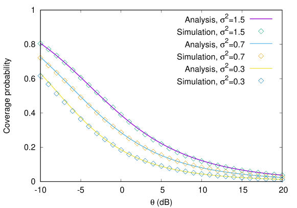
Figure 1: Coverage probability in the TPP network with $\lambda_{p}=0.1/\pi$, $\alpha=10$.

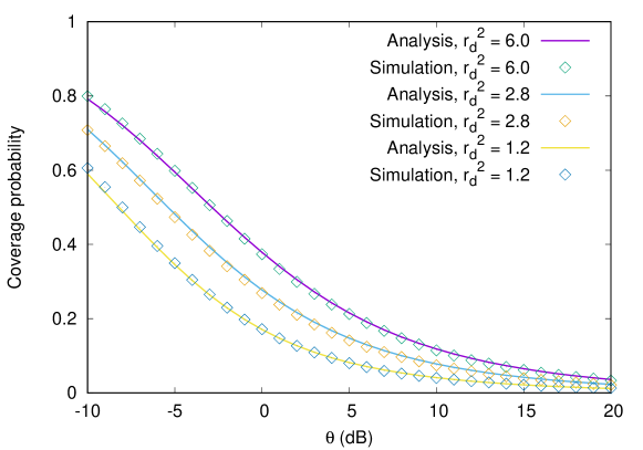
Figure 2: Coverage probability in the MCP network with $\lambda_{p}=0.1/\pi$, $\alpha=10$.

We should notice that the actual numerical computation of the coverage probability using (9) is not so easy. In particular, the integral inside function $M$ in Theorem 1 hardly converges in a numerical sense (though the finite existence is ensured in the proof of Theorem 1) and we should take a truncation technique carefully.

5 Conclusion

We have considered a spatial downlink cellular network model with BSs deployed according to a PPCP and, within the most fundamental setup such as single-tier, Rayleigh fading and nearest BS association, we have derived the coverage probability in a numerically computable form. This work does not only fill in a hole of the literature but also is expected to play a role of a building block for analysis of, for example, HetNets with a tier consisting of open access small cell BSs.

References

- [1] B. Błaszczyszyn and D. Yogeshwaran, “Clustering comparison of point processes with applications to random geometric models,” in Stochastic Geometry, Spatial Statistics and Random Fields: Models and Algorithms, V. Schmidt, Ed. Springer, 2014, pp. 31–71.
- [2] V. Suryaprakash, J. Møller, and G. Fettweis, “On the modeling and analysis of heterogeneous radio access networks using a Poisson cluster process,” IEEE Transactions on Wireless Communications, vol. 14, pp. 1035–1047, 2015.
- [3] N. Deng, W. Zhou, and M. Haenggi, “Heterogeneous cellular network models with dependence,” IEEE Journal on Selected Areas in Communications, vol. 33, pp. 2167–2181, 2015.
- [4] Y. J. Chun, M. O. Hasna, and A. Ghrayeb, “Modeling heterogeneous cellular networks interference using Poisson cluster processes,” IEEE Journal on Selected Areas in Communications, vol. 33, pp. 2182–2195, 2015.
- [5] C. Saha, M. Afshang, and H. S. Dhillon, “3GPP-inspired HetNet model using Poisson cluster process: Sum-product functionals and downlink coverage,” IEEE Transactions on Communications, 2017, in press.
- [6] M. Afshang and H. S. Dhillon, “Poisson clustered process based analysis of HetNets with correlated user and base station locations,” IEEE Transactions on Wireless Communications, 2018, in press.
- [7] M. Afshang, H. S. Dhillon, and P. H. J. Chong, “Modeling and performance analysis of clustered device-to-device networks,” IEEE Transactions on Wireless Communications, vol. 15, pp. 4957–4972, 2016.
- [8] W. Yi, Y. Liu, and A. Nallanathan, “Modeling and analysis of D2D millimeter-wave networks with Poisson cluster processes,” IEEE Transactions on Communications, vol. 65, pp. 5574–5588, 2017.
- [9] S. Joshi and R. K. Mallik, “Coverage and interference in D2D with Poisson cluster process,” IEEE Communications Letters, 2018, in press.
- [10] M. Afshang, C. Saha, and H. S. Dhillon, “Nearest-neighbor and contact distance distributions for Thomas cluster process,” IEEE Wireless Communications Letters, vol. 6, pp. 130–133, 2017.
- [11] ——, “Nearest-neighbor and contact distance distributions for Matérn cluster process,” IEEE Communications Letters, vol. 21, pp. 2686–2689, 2017.
- [12] B. Błaszczyszyn, M. Haenggi, P. Keeler, and S. Mukherjee, Stochastic Geometry Analysis of Cellular Networks. Cambridge University Press, 2018.
- [13] S. N. Chiu, D. Stoyan, W. S. Kendall, and J. Mecke, Stochastic Geometry and its Applications, 3rd ed. Wiley, 2013.
- [14] J. Proakis and M. Salehi, Digital Communications, 5th ed. McGraw-Hill, 2007.
- [15] J. G. Andrews, F. Baccelli, and R. K. Ganti, “A tractable approach to coverage and rate in cellular networks,” IEEE Transactions on Communications, vol. 59, pp. 3122–3134, 2011.
- [16] U. Schilcher, S. Toumpis, M. Haenggi, A. Crismani, G. Brandner, and C. Bettstetter, “Interference functionals in Poisson networks,” IEEE Transactions on Information Theory, vol. 62, pp. 370–383, 2016.
- [17] D. J. Daley and D. Vere-Jones, An Introduction to the Theory of Point Processes: Volume II: General Theory and Structure, 2nd ed. Springer, 2008.
- [18] Y. Takahashi, Y. Chen, T. Kobayashi, and N. Miyoshi, “Simple and fast PPP-based approximation of SIR distributions in downlink cellular networks,” 2017, submitted.