Smoothing for signals with discontinuities
using higher order Mumford-Shah models

Abstract

Minimizing the Mumford-Shah functional is frequently used for smoothing signals or time series with discontinuities. A significant limitation of the standard Mumford-Shah model is that linear trends – and in general polynomial trends – in the data are not well preserved. This can be improved by building on splines of higher order which leads to higher order Mumford-Shah models. In this work, we study these models in the univariate situation: we discuss important differences to the first order Mumford-Shah model, and we obtain uniqueness results for their solutions. As a main contribution, we derive fast minimization algorithms for Mumford-Shah models of arbitrary orders. We show that the worst case complexity of all proposed schemes is quadratic in the length of the signal. Remarkably, they thus achieve the worst case complexity of the fastest solver for the piecewise constant Mumford-Shah model (which is the simplest model of the class). Further, we obtain stability results for the proposed algorithms. We complement these results with a numerical study. Our reference implementation processes signals with more than 10,000 elements in less than one second.

Keywords: piecewise smooth approximation, discontinuous signals, complexity penalized estimation, changepoint estimation, segmented least squares, spline smoothing, Mumford-Shah model, Potts model, Blake-Zisserman model.

AMS subject classification (MSC2010): 65D10, 65K05, 62G08, 65K10, 65D07.

1 Introduction

Smoothing is an important processing step when working with measured signals or time series. For signals without discontinuities, it is standard to use smoothing splines for this task. In various applications however, the signals possess discontinuities. Such applications are, for example, the cross-hybridization of DNA [56, 20, 32], the reconstruction of brain stimuli [74], single-molecule fluorescence resonance energy transfer [36], cellular ion channel functionalities [31], photo-emission spectroscopy [25] and the rotations of the bacterial flagellar motor [57]; see also [43, 44, 25] for further examples. Frequently, it is important to preserve the discontinuities since they typically indicate a significant change. Unfortunately, the locations of the discontinuities are in general unknown; they have to be estimated along with the signal.

One approach to this problem is to estimate the discontinuities locally and adapt the corresponding fitting operator to the local situation in an explicit way; for instance [3, 1, 29]. Other approaches use variational methods: an energy functional is considered and a corresponding minimizer yields a smoothed approximation to the data. Examples for discontinuity preserving methods are total variation (TV)/Rudin-Osher-Fatemi models [55] which yield a kind of piecewise constant approximation. To account for linear and higher order trends in the data, higher order TV methods have been proposed [16, 11]. TV models and their higher order extensions, however, do not explicitly incorporate the notion of discontinuities and segment boundaries. A model taking these notions explicitly into account is the Mumford-Shah model. It simultaneously estimates a discontinuity set and a corresponding piecewise smooth approximation [47]. Its piecewise constant variant is also known as the Potts model [49, 27, 72], or as the Chan-Vese model for the case of two phases [17]. Mumford-Shah and Potts models are classical models for discontinuity preserving smoothing and for segmentation [8, 27, 46, 72]. More recent applications are smoothing of video sequences [61] and segmentation with shape priors [33]. They are also used for stabilizing the reconstructions of inverse problems [54, 53, 35, 50, 51, 67]. Corresponding existence results on minimizers were established in [4, 23]. Besides the classical $\ell^{2}$-based models, $\ell^{p}$-based variants with $p\geq 1$ [22, 30, 40, 26, 68, 58] and manifold-valued data spaces [66, 69, 58] have been considered. Discretizations have been studied in [14, 15]. Mumford-Shah and Potts problems are known to be NP hard in the multivariate case and in the univariate inverse problem setup [63, 10, 67]. Approximate solution strategies are for example based on graduated non-convexity [8, 9], approximation by elliptic functionals [2, 54, 6], graph cuts [10], active contours [62], convex relaxations [60], iterative thresholding algorithms [22], ADMM splitting schemes [59, 30], and iterative Potts minimization [67, 37]. In the univariate case, dynamic programming strategies yield exact solutions as discussed in more detail later on.

A significant limitation of the classical Mumford-Shah model is that it does not well preserve locally linear or polynomial trends in the data. Instead, it tends to produce spurious discontinuities when the slope of the signal is too high, which has been termed the “gradient limit effect” by Blake and Zisserman [8]. The reason for this is that it penalizes deviations from a piecewise constant spline. The preservation of linear or polynomial trends can be accomplished by considering higher order Mumford-Shah models. They penalize the deviation from a piecewise polynomial instead of the deviation from a piecewise constant function. The multivariate discrete higher order Mumford-Shah and Potts models are particularly interesting in image processing for edge preserving smoothing of images with locally linear or polynomial trends; for example, second order methods are applied for piecewise approximation and segmentation of images [65, 77, 18, 78] or regularization of flow fields [76, 24]. The univariate discrete models are particularly interesting for smoothing time series with discontinuities; examples with biological applications are for instance [48, 57]. Further they arise as subproblems in univariate and multivariate splitting schemes [59, 30, 67, 37].

We intend to systematically study higher order Mumford-Shah models, where, in this paper, we consider the univariate and discrete situation. It is given by the minimization problem

$$(u^{*},\mathcal{I}^{*})=\operatorname*{argmin}_{u\in\mathbb{R}^{N},~{}\mathcal{I}\text{ partition}}~{}\|u-f\|_{2}^{2}+\sum_{I\in\mathcal{I}}\beta^{2k}\|\nabla^{k}u_{I}\|_{2}^{2}+\gamma\,|\mathcal{I}|. \mathcal{P}_{k,\beta,\gamma}$$ ()

Here, $f\in\mathbb{R}^{N}$ denotes the given data, and the minimum is computed with respect to the target variables $u$ and $\mathcal{I},$ where $u$ is a discrete univariate signal of length $N$ and $\mathcal{I}$ is a partition of the domain $\Omega=\{1,\ldots,N\}.$ (The connection between $u$ and $\mathcal{I}$ is discussed in detail later in Section 2.2.) The symbol $\nabla^{k}u_{I}$ denotes the $k$-th order finite difference operator applied to the vector $u$ restricted to the “interval” $I$ of a partition $\mathcal{I}$ of the domain. The functional value comprises a cost term for the data deviation, a cost term for the inner energy of a spline on the single segments, and a cost term for the complexity of the partition (measured in terms of the number of segments $|\mathcal{I}|$). The minimizing signal $u^{*}$ is a piecewise $k$-th order discrete spline approximation to $f$ with elasticity parameter $\beta$ which has discontinuities or breakpoints at the boundaries given by the partition $\mathcal{I}^{*}.$ Choosing a large parameter value $\beta$ leads to stronger smoothing on the segments, and choosing a large parameter value $\gamma$ leads to less segments. It is interesting to look at the cases for very large parameters of $\beta$ and $\gamma.$ As the kernel of $\nabla^{k}$ consists of polynomials of maximum degree $k-1,$ the limit situation $\beta\to\infty$ can be written as

$$\operatorname*{argmin}_{u,\mathcal{I}}~{}\|u-f\|_{2}^{2}+\gamma\,|\mathcal{I}|,\quad\text{s.t. $u_{I}$ is a polynomial of maximum degree $k-1$ for all $I\in\mathcal{I}.$} \mathcal{P}_{k,\infty,\gamma}$$ ()

As the case $k=1$ is known as the Potts model (as a tribute to the work of R. Potts [49]) we refer to ($\mathcal{P}_{k,\infty,\gamma}$) as higher order Potts model. On the other hand, for sufficiently large $\gamma,$ it reduces to the (discrete) $k$-th order spline approximation

$$\operatorname*{argmin}_{u}~{}\|u-f\|_{2}^{2}+\beta^{2k}\|\nabla^{k}u\|_{2}^{2}, \mathcal{P}_{k,\beta,\infty}$$ ()

which is a classical method for smoothing data; see [70, 64]. Depending on the application, there are different points of view for Mumford-Shah-type models: On the one hand, the optimal partition $\mathcal{I}^{*}$ can serve as a basis for identifying segment neighborhoods [5] and as an indicator for changepoints of the signal [38]. On the other hand, the corresponding optimal signal $u^{*}$ can serve as a smoother for a signal with discontinuities [8, 73].

In the literature, the members of the higher order Mumford-Shah family ($\mathcal{P}_{k,\beta,\gamma}$) have been considered for the cases $k=1,2$ and for $\beta<\infty$ or $\beta=\infty$ (strict piecewise polynomial model) by various individual studies. The classical (first order) Potts model $(\mathcal{P}_{1,\infty,\gamma})$ and closely related models were studied in various works; for example [12, 42, 73, 75, 38]. The strict piecewise linear model $(\mathcal{P}_{2,\infty,\gamma})$ was studied by Bellman and Roth [7]; see also [39]. We refer to it as affine Potts model or piecewise affine Mumford-Shah model. The first order problems $(\mathcal{P}_{1,\beta,\gamma})$ for arbitrary parameters $\beta$ have been studied in the seminal works of Mumford and Shah [46, 47]. (This motivates the denomination higher order Mumford-Shah model for the family ($\mathcal{P}_{k,\beta,\gamma}$).) The same problem was studied at around the same time by Blake and Zisserman [8] under the name weak string model. They also introduced a second order extension, called the weak rod model [8]. This model is more general than the model $(\mathcal{P}_{2,\beta,\gamma})$ considered here because it has an extra penalty for discontinuities in the first derivative. We refer to [13, 78] for a recent investigation of Blake-Zisserman models in 2D. To our knowledge, the models $(\mathcal{P}_{k,\beta,\gamma})$ have not been systematically studied for arbitrary orders $k.$

Although ($\mathcal{P}_{k,\beta,\gamma}$) is a non-convex problem it can be solved exactly by dynamic programming; see [7, 9, 5, 73, 34, 26]. The state-of-the-art solver has worst case complexity $O(N^{2}\phi(N))$ where $\phi(N)$ comprises the costs of computing a spline approximation error on an interval of maximum length $N$; see [73, 39, 26]. Killick et al. [38] proposed a pruning strategy to accelerate the algorithm in a special yet practically relevant case: if the expected number of segments $|\mathcal{I}^{*}|$ grows linearly in $N$ and if the expected log-likelihood fulfills certain estimates, detailed in [38], the expected complexity is $\mathcal{O}_{P}(N\phi(N)).$ Another pruning scheme has been established in [59]. An algorithm for solving the first order Mumford-Shah problem for all parameters $\gamma$ simultaneously was proposed in [26]. It is straightforward to devise an algorithm for $(\mathcal{P}_{k,\beta,\gamma})$ of complexity $\mathcal{O}(N^{3}).$ For the first order problem $(\mathcal{P}_{1,\beta,\gamma}),$ we proposed an $\mathcal{O}(N^{2})$ algorithm [30] which utilizes a fast computation scheme for the approximation errors proposed by Blake [9]. Unfortunately, as that scheme is based on algebraic recurrences, a generalization to arbitrary orders of $k$ seems difficult. By precomputations of moments one can achieve $\phi(N)=\mathcal{O}(1);$ see [41, 26]. Although that approach gives reasonable results for the low orders $k=1,2,$ it gets numerically unstable for higher orders. A different dynamic programming approach was discussed in [8] which however only computes an approximate minimizer.

Contribution.

This work deals with the analysis and with solvers for the higher order Mumford-Shah and Potts problems ($\mathcal{P}_{k,\beta,\gamma}$). First, we discuss basic properties of higher order Mumford-Shah models, we prove that the solutions are unique for almost all input data, and we discuss connections with related models. A main contribution is a fast non-iterative algorithm for minimizing the higher-order Mumford-Shah and Potts models of arbitrary order. The proposed schemes are based on dynamic programming and recurrence relations. We prove that the proposed algorithms have the same worst case complexity as the state-of-the-art solver for minimizing the (simpler) piecewise constant Mumford-Shah model, i.e., their runtime grows quadratically with respect to the length of the signal. Our reference implementation processes signals of length over 10,000 in less than one second on a standard desktop computer. Further, we derive stability results for the proposed algorithms. Eventually, we provide a numerical study where we in particular compare with the first order model with respect to runtime and reconstruction quality.

Organization of the paper.

In Section 2 we describe and discuss higher order Mumford-Shah and higher order Potts models. In Section 3, we develop a fast solver for higher order Mumford-Shah problems and for higher order Potts problems, and we analyze the stability. A numerical study is given in Section 4.

2 Higher order Mumford-Shah and Potts models

We start with some basic notations and definitions. Our goal is to recover an unknown signal $g\in\mathbb{R}^{N}$ from its noisy samples

$$f_{n}=g_{n}+\eta_{n},\quad\text{}n=1,...,N,$$ (1)

where the $\eta_{n}$ are independently distributed Gaussian random variables of zero mean and variance $\sigma^{2}.$ We write ${l:r}$ for a discrete “interval” from $l$ to $r$, i.e. ${l:r}=\{l,l+1,\ldots r\}.$ It is convenient to use the Matlab-type notation $x_{I}=x_{l:r}=(x_{l},x_{l+1},\ldots,x_{r})$ for indexing. We say that $\mathcal{I}$ is a partition of $\Omega={1:N}$ into intervals, if $I\cap J=\emptyset$ for all $I,J\in\mathcal{I},$ if $\bigcup_{I\in\mathcal{I}}I=\Omega,$ and if all $I\in\mathcal{I}$ are discrete intervals of the form $I={l:r},$ with $1\leq l\leq r\leq N.$ As we will only work with partitions into intervals here, we briefly call $\mathcal{I}$ a partition. Further, we use the notation $\|u\|_{2}^{2}=\sum_{n=1}^{N}u_{n}^{2}$ for $u\in\mathbb{R}^{N}$ to denote the squared Euclidean length of $u.$

2.1 First order Mumford-Shah models and the gradient limit effect

Before considering higher order models, we first review some important properties of first order models. The first order Mumford-Shah problem ($\mathcal{P}_{1,\beta,\gamma}$) on the discrete domain $\Omega$ can be written as

$$(u^{*},\mathcal{I}^{*})=\operatorname*{argmin}_{u\in\mathbb{R}^{N},\,\mathcal{I}\text{ partition of }\Omega}~{}\sum_{n=1}^{N}(u_{n}-f_{n})^{2}+\beta^{2}\sum_{I\in\mathcal{I}}\sum_{i=1}^{|I|-1}((u_{I})_{i+1}-(u_{I})_{i})^{2}+\gamma\,|\mathcal{I}|.$$ (2)

The two-fold minimization with respect to the signal $u$ and the partition $\mathcal{I}$ is instructive but cumbersome in practice. We can remove the explicit dependance on the signal $u.$ The formulation in terms of partitions reads

$$\mathcal{I}^{*}=\operatorname*{argmin}_{\mathcal{I}\text{ partition of }{1:N}}\sum_{I\in\mathcal{I}}\Big{(}\mathcal{E}^{I}+\gamma\Big{)},\quad\text{with }\mathcal{E}^{I}=\min_{v\in\mathbb{R}^{|I|}}~{}\sum_{i=1}^{|I|}(v_{i}-f_{i})^{2}+\beta^{2}\sum_{I\in\mathcal{I}}\sum_{i=1}^{|I|-1}(v_{i+1}-v_{i})^{2}.$$ (3)

Here $\mathcal{E}^{I}$ describes the error of the best first order discrete spline approximation on the interval $I.$ This formulation is typically used for derivation of algorithms based on dynamic programming [9, 26].

For the first order model (2), it is possible to rewrite the functional without partitions. The corresponding formulation reads

$$u^{*}=\operatorname*{argmin}_{u\in\mathbb{R}^{N}}~{}\sum_{n=1}^{N}(u_{n}-f_{n})^{2}+\sum_{n=1}^{N-1}\min(\beta^{2}(u_{n+1}-u_{n})^{2},\gamma).$$ (4)

This formulation is useful for derivation of algorithms based on iterative thresholding techniques [22]. The key property that makes the formulation in terms of $u$ possible is that, for the first order model, the signal $u^{*}$ and the partition $\mathcal{I}^{*}$ are equivalent in the sense that $\mathcal{I}^{*}$ can be recovered from $u^{*}$ and vice-versa.

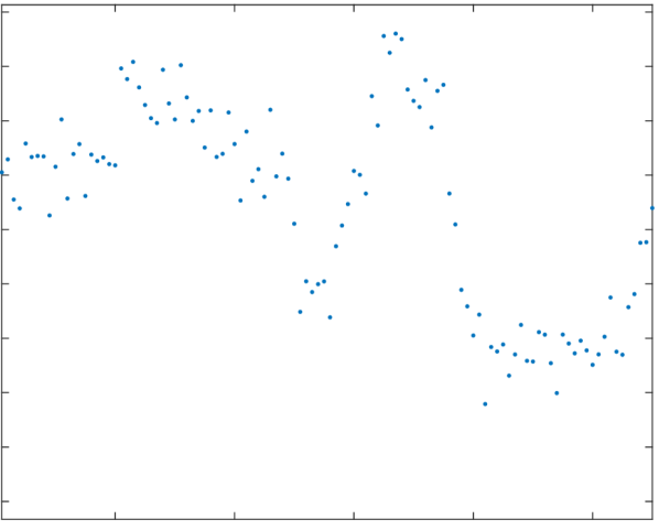
(a) Noisy signal with discontinuities

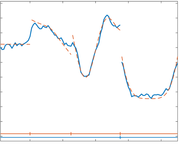
(b) Result of $(\mathcal{P}_{1,\beta,\gamma})$ with optimal $\beta,\gamma$

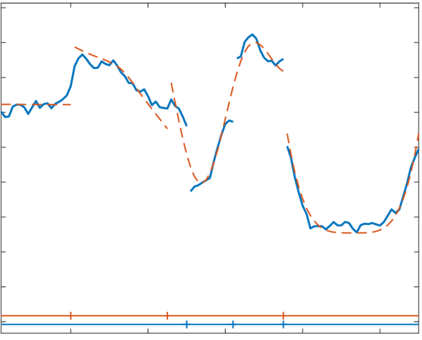
(c) Smaller complexity penalty $\gamma$

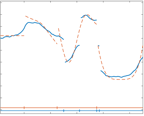
(d) Larger elasticity parameter $\beta$

Figure 1: Limitations of the classical (first order) Mumford-Shah model: Subfigures (b) to (d) show reconstructions of the signal in (a) by the first order Mumford-Shah model $(\mathcal{P}_{1,\beta,\gamma}).$ The red dashed lines depict the ground truth; the streaks at the bottom indicate the discontinuities or segments of the ground truth (top, red) and the computed segmentations (bottom, blue). (b) The model parameters were optimized with respect to the $\ell^{2}$ error to the ground truth ($\gamma=0.04$, $\beta=1.3625$). The result provides unsatisfactory smoothing and detection of discontinuities. (c) Decreasing the complexity penalty (here $\gamma=0.02$) leads to more but dislocated discontinuities. (d) Increasing the elasticity parameter (here $\beta=3$) leads to stronger smoothing, but to spurious segments as well. In either case, the first order model shows the tendency to create spurious discontinuities at steep slopes which is known as the gradient limit effect.

As mentioned in the introduction, a major limitation of the classical Mumford-Shah model is that data with locally linear or polynomial trends are not well approximated. This undesirable effect, known as gradient limit effect, is illustrated in Figure 1. We observe that the solution of the first order model (using model parameters optimized to the $\ell^{2}$ error) does not catch all discontinuities. We also see that tuning the model parameters towards allowing for more discontinuities leads to spurious discontinuities at steep slopes. This shows that the first order models are not rich enough for dealing with data having locally linear or polynomial trends.

2.2 Basic properties of higher order Mumford-Shah and Potts models

We denote by $\nabla^{k}\in\mathbb{R}^{(q-k)\times q}$ the matrix that acts as $k$-th order finite difference on the vector $u_{I}$ where $q=|I|.$ To fix ideas, the matrices $\nabla^{k}$ are given for $k=1$ and $k=2$ by

$$\nabla=\begin{pmatrix}-1&1&&&\\ &-1&1&&\\ &&\ddots&\ddots&\\ &&&-1&1\\ \end{pmatrix}\in\mathbb{R}^{(q-1)\times q}\qquad\text{and}\quad\nabla^{2}=\begin{pmatrix}1&-2&1&&&\\ &1&-2&1&&\\ &&\ddots&\ddots&\ddots&\\ &&&1&-2&1\\ \end{pmatrix}\in\mathbb{R}^{(q-2)\times q}.$$

For higher orders $k\geq 3,$ the row pattern is equal to $t*t*\ldots*t$ which denotes the $k$-fold convolution of the finite difference vector $t=(-1,1)$ with itself.

Using this notation the higher order Mumford-Shah problem ($\mathcal{P}_{k,\beta,\gamma}$) can be written as

$$(u^{*},\mathcal{I}^{*})=\operatorname*{argmin}_{u\in\mathbb{R}^{N},\,\mathcal{I}\text{ partition of }\Omega}~{}\underbrace{\sum_{n=1}^{N}(u_{n}-f_{n})^{2}}_{\text{data penalty}}+\underbrace{\beta^{2k}\sum_{I\in\mathcal{I}}\sum_{i=1}^{|I|-k}(\nabla^{k}u_{I})_{i}^{2}}_{\text{smoothness penalty}}+\underbrace{\gamma\,|\mathcal{I}|.}_{\text{complexity penalty}}$$ (5)

As mentioned in the introduction, the functional comprises a data penalty term, a smoothness penalty term, and a complexity penalty term. A minimizer $u^{*}$ is a $k$-th order discrete spline approximation to data $f$ on each segment of the partition $\mathcal{I}^{*}.$ The parameter $\gamma$ determines the penalty for opening a new segment. The parameter $\beta$ controls influence of the smoothness penalty. The order $k$ is the derivative order of the (discrete) spline. Note that polynomials of order $k-1$ on a segment do not have any smoothness penalty.

An illustration on the smoothing effect of higher order Mumford-Shah models in comparison to classical splines and to first order models is given in Figure 2.

(a) Noisy signal with discontinuities

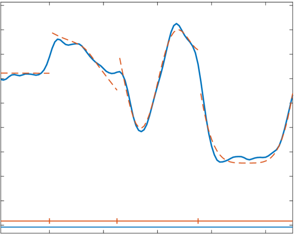
(b) Smoothing spline

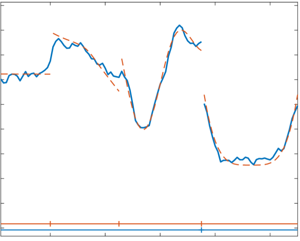
(c) Classical Mumford-Shah $(\mathcal{P}_{1,\beta,\gamma})$

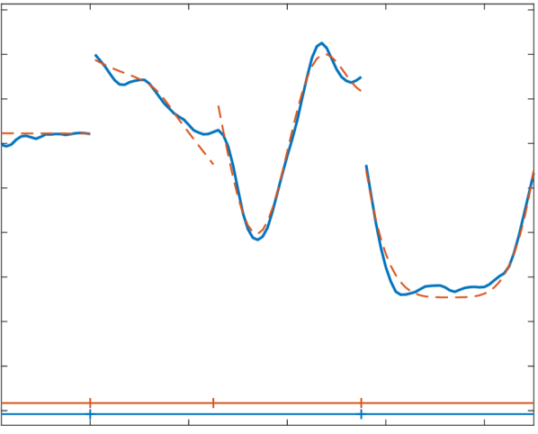
(d) Higher order Mumford-Shah $(\mathcal{P}_{2,\beta,\gamma})$

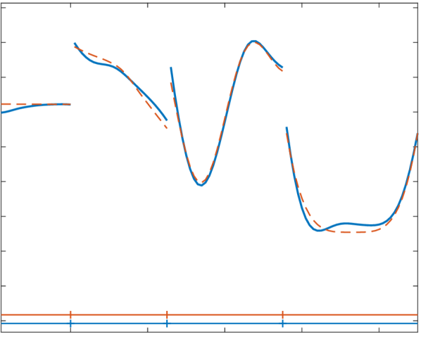
(e) Higher order Mumford-Shah $(\mathcal{P}_{3,\beta,\gamma})$

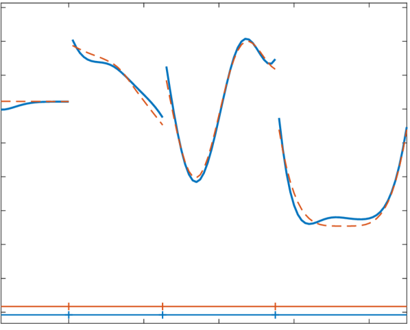
(f) Higher order Mumford-Shah $(\mathcal{P}_{4,\beta,\gamma})$

Figure 2: Smoothing a noisy signal with discontinuities using various models. All model parameters are chosen with respect to optimal $\ell^{2}$-error. As in Figure 1, the ground truth is depicted as red dashed line and the estimate as blue solid line. (b) Classical spline approximation smoothes out the discontinuities. (c) The classical Mumford-Shah model allows for discontinuities, but the estimate misses most of them and the result remains noisy. (d–f) The higher order Mumford-Shah results provide improved smoothing and segmentation. In particular, the third and the fourth order models get the discontinuities of the groundtruth.

Formulation as partitioning problem.

As in the first order case, it is convenient to formulate the higher order Mumford-Shah problem (5) in terms of the partition only; it reads

$$\mathcal{I}^{*}=\operatorname*{argmin}_{\mathcal{I}\text{ partition of }{1:N}}\sum_{I\in\mathcal{I}}(\mathcal{E}^{I}+\gamma),$$ (6)

where $\mathcal{E}^{I}$ denotes the approximation error of the $k$-th order (discrete) smoothing spline on $I$ given by

$$\mathcal{E}^{I}=\min_{v\in\mathbb{R}^{|I|}}~{}\|v-f_{I}\|_{2}^{2}+\beta^{2k}\|\nabla^{k}v\|_{2}^{2}=\min_{v\in\mathbb{R}^{|I|}}~{}\sum_{i=1}^{|I|}(v_{i}-(f_{I})_{i})^{2}+\sum_{i=1}^{|I|-k}\beta^{2k}(\nabla^{k}v)_{i}^{2}.$$ (7)

Note that the $k$-th order finite difference $\nabla^{k}$ is only well defined for vectors of length greater than $k,$ so $\mathcal{E}^{I}=0$ if $|I|\leq k.$ The minimizing estimate $u^{*}$ can be recovered from an optimal partition $\mathcal{I}^{*}$ by solving

$$u_{I}^{*}=\operatorname*{argmin}_{v\in\mathbb{R}^{|I|}}~{}\|v-f_{I}\|_{2}^{2}+\beta^{2}\|\nabla^{k}v\|_{2}^{2},\quad\text{ for all }I\in\mathcal{I}^{*}.$$ (8)

Hence, if we have computed an optimal partition $\mathcal{I}^{*}$ of the domain $\Omega,$ its accompanying signal estimate $u^{*}$ is uniquely determined.

To express the relation between $u^{*}$ and $\mathcal{I}^{*},$ it is convenient to introduce a formulation in terms of block matrices. A partition $\mathcal{I}$ defines a block diagonal matrix $L_{\mathcal{I}}$ by

$$L_{\mathcal{I}}=\begin{pmatrix}L_{|\mathcal{I}_{1}|}&&&\\ &L_{|\mathcal{I}_{2}|}&&\\ &&\ddots&\\ &&&L_{|\mathcal{I}_{M}|}\end{pmatrix},\qquad\text{with}\qquad L_{n}=\nabla^{k}\in\mathbb{R}^{(n-k)\times n},$$ (9)

and with $k$-th order finite difference matrices $\nabla^{k}$ of the appropriate size $(n-k)\times n$ defined as above. Here, $|\mathcal{I}_{m}|$ denotes the cardinality of the $m$-th element of the partition $\mathcal{I}.$ If $n\leq k,$ we use the convention that $L_{n}$ is an “empty” block of length $n.$ The number of columns of $L_{\mathcal{I}}$ is equal to $N,$ and the number of rows depends on the size of the intervals with minimum length $k+1$ of the partition, i.e., $\sum_{m=1}^{M}\max(|I_{m}|-k,0).$ For example, for $k=2$ the partition $\mathcal{I}=\{(1,\ldots,4),(5,6),(7,\ldots,9)\}$ defines the matrix

$$L_{\mathcal{I}}=\begin{pmatrix}1&-2&1&&&&&\\ &1&-2&1&&&&&\\ &&&&&&1&-2&1\\ \end{pmatrix}\in\mathbb{R}^{3\times 9}.$$

The block matrix notation (9) allows to formulate the minimization problem (5) in the compact form

$$\operatorname*{argmin}_{u\in\mathbb{R}^{N},\,\mathcal{I}\text{ partition}}~{}\beta^{2k}\,\|L_{\mathcal{I}}u\|_{2}^{2}+\|u-f\|_{2}^{2}+\gamma\,|\mathcal{I}|.$$ (10)

For a fixed partition $\mathcal{I},$ taking derivatives with respect to $u$ reveals that a minimizer $u_{\mathcal{I}}$ satisfies the linear system

$$2\beta^{2k}L_{\mathcal{I}}^{T}L_{\mathcal{I}}u_{\mathcal{I}}+2(u_{\mathcal{I}}-f)=0.$$ (11)

As the system has full rank for all $\beta\geq 0$ we get the unique solution

$$u_{f,\mathcal{I}}=S_{\mathcal{I},\beta}f,\qquad\text{where }S_{\mathcal{I},\beta}=(\beta^{2k}L_{\mathcal{I}}^{T}L_{\mathcal{I}}+\mathrm{id})^{-1}.$$ (12)

We omit the subscript if the dependence on $\mathcal{I}$ or $\beta$ is clear. Plugging (12) into (5) gives the explicit expression for the functional value of the higher order Mumford-Shah functional restricted to the partition $\mathcal{I}$ as

$$\mathcal{G}^{\prime}_{\mathcal{I}}(f)=\beta^{2k}\,\|L_{\mathcal{I}}S_{\mathcal{I}}f\|_{2}^{2}+\|S_{\mathcal{I}}f-f\|_{2}^{2}+\gamma\,|\mathcal{I}|.$$ (13)

Hence, the minimizing partition $\mathcal{I}^{*}$ is given as the minimizing argmuent of $\mathcal{I}\mapsto\mathcal{G}^{\prime}_{\mathcal{I}}(f).$

In contrast to the first order model, expressing the problem only in terms of $u$ just like in (4) is not feasible. A reason for this is that one solution $u$ may be the result of different partitions with different numbers of segments. A simple example is the data $f=(0,1,0).$ For $\gamma<2/3$ and for $\beta$ sufficiently large, a minimizer is given by $u=f.$ The partitions $\big{\{}(1,2),(3)\big{\}},$ $\big{\{}(1),(2,3)\big{\}}$ and $\big{\{}(1),(2),(3)\big{\}}$ lead to this $u=f.$

Minimum functional values and minimum segment lengths.

We record the following basic property about minimizers. Its proof follows an argument similar to the one used in [8] for a continuous domain second order problem.

Lemma 1.

Let $\mathcal{I}^{*}$ be a minimizing partition of (5). Then the minimal functional value is given by

$$\mathcal{G}^{\prime}_{\mathcal{I}^{*}}(f)=\|f\|_{2}^{2}-f^{T}S_{\mathcal{I}^{*},\beta}f+\gamma\,|\mathcal{I}^{*}|.$$

Proof.

Let $\tilde{u}=S_{\mathcal{I}^{*},\beta}f.$ Expanding the functional yields

$$\begin{split}\mathcal{G}^{\prime}_{\mathcal{I}^{*}}(f)&=\beta^{2k}\|L_{\mathcal{I}^{*}}\tilde{u}\|_{2}^{2}+\|\tilde{u}-f\|_{2}^{2}+\gamma\,|\mathcal{I}^{*}|\\ &=\beta^{2k}\tilde{u}^{T}L_{\mathcal{I}^{*}}^{T}L_{\mathcal{I}^{*}}\tilde{u}+(\tilde{u}-f)^{T}(\tilde{u}-f)+\gamma\,|\mathcal{I}^{*}|\\ &=\beta^{2k}\tilde{u}^{T}L_{\mathcal{I}^{*}}^{T}L_{\mathcal{I}^{*}}\tilde{u}+\tilde{u}^{T}(\tilde{u}-f)+f^{T}(\tilde{u}-f)+\gamma\,|\mathcal{I}^{*}|\\ &=\tilde{u}^{T}(\beta^{2k}L_{\mathcal{I}^{*}}^{T}L_{\mathcal{I}^{*}}\tilde{u}+(\tilde{u}-f))-f^{T}(\tilde{u}-f)+\gamma\,|\mathcal{I}^{*}|\\ &=-f^{T}(\tilde{u}-f)+\gamma\,|\mathcal{I}^{*}|=\|f\|_{2}^{2}-f^{T}\tilde{u}+\gamma\,|\mathcal{I}^{*}|,\end{split}$$

where we used the minimality property (11) in the penultimate line. ∎

Next we show that there is always an optimal partition $\mathcal{I}^{*}$ which has at most one segment with less than $k$ elements:

Lemma 2.

For each partition $\mathcal{I}$ there is a partition $\mathcal{I}^{\prime}$ such that all segments $I^{\prime}\in\mathcal{I}^{\prime}$ (except possibly the leftmost one) have length greater or equal than $k$ and that

$$\sum_{I^{\prime}\in\mathcal{I}^{\prime}}\mathcal{E}^{I^{\prime}}\leq\sum_{I\in\mathcal{I}}\mathcal{E}^{I}\quad\text{and}\quad|\mathcal{I}^{\prime}|\leq|\mathcal{I}|.$$

In particular $\mathcal{G}^{\prime}_{\mathcal{I}^{\prime}}(f)\leq\mathcal{G}^{\prime}_{\mathcal{I}}(f).$

Proof.

Let $\mathcal{I}$ be a partition and let $I$ be its right-most segment such that $|I|<k.$ Denote by $i$ the left boundary index of $I$. If $i=1$ we are done. Otherwise, we transfer the element $i-1$ from the left neighboring segment to the segment $I$ and denote the partition modified in this way by $\mathcal{I}^{\prime}.$ (If the neighboring segment gets empty, we remove it from the partition.) On the one hand, $|\mathcal{I}^{\prime}|\leq|\mathcal{I}|.$ On the other hand, since $|I\cup\{i-1\}|\leq k$ we have that $\mathcal{E}^{I\cup\{i-1\}}=0.$ Repeating the above procedure a finite number of times, we end up with a partition $\mathcal{I}^{\prime\prime}$ whose segments have length greater or equal to $k,$ except possibly the leftmost segment. ∎

Higher order Potts models.

As mentioned in the introduction, the higher order Potts model ($\mathcal{P}_{k,\infty,\gamma}$) can be seen as the limit case of the higher order Mumford-Shah model for $\beta\to\infty.$ The main difference to the higher order Mumford-Shah model is that the approximation on a segment is performed by a polynomial of maximum degree $k-1$ instead of a $k$-th order spline. In consequence, the approximation error on a segment $I={l:r}$ is given by

$$\mathcal{E}^{I}=\min_{\begin{subarray}{c}v\text{ polynomial of}\\ \text{degree $\leq k-1$ on }I\end{subarray}}\|v-f_{I}\|_{2}^{2}.$$ (14)

Complementing (7) for the Mumford-Shah problem, (14) is a least squares problem in the coefficients of the polynomial.

On the one hand, higher order Potts models are more restrictive than genuine higher order Mumford-Shah models since they enforce piecewise polynomial solutions. On the other hand, due to the stronger prior, they are more robust to noise. From the computational side, one parameter less has to be determined for the Potts model.

Being the limit case $\beta\to\infty,$ the higher order Potts models has similar properties as the Mumford-Shah model. In particular, if the data can be described by a polynomial of order $k-1$ on a segment, then that segment does not get any approximation penalty. In consequence, the assertion of Lemma 2 holds true for the higher order Potts models as well.

2.3 Existence and uniqueness of minimizers

It is straightforward to show the existence of minimizers.

Theorem 3.

The higher-order Mumford-Shah/Potts model ($\mathcal{P}_{k,\beta,\gamma}$) has a minimizer for each $k\in\mathbb{N},$ $\gamma>0,$ $\beta\in(0,\infty].$

Proof.

For a fixed partition $\mathcal{I}$, the problem ($\mathcal{P}_{k,\beta,\gamma}$) reduces to least squares problems on the intervals of $\mathcal{I}$ which all possess minimizers. As there are only finitely many partitions on $\Omega,$ there is at least one solution with a minimal functional value. ∎

Uniqueness of the solution is more intricate. The next example shows that the solutions of the higher order Mumford-Shah models ($\mathcal{P}_{k,\beta,\gamma}$) need not be unique. For simplicity, we consider only the case $k=2,$ but analogous examples can be given for any order $k\geq 3.$

Example 4.

Consider data $f=(0,1,0)$ and $k=2.$ The optimal signal corresponding to the partition $\mathcal{I}^{3}=\{(1),(2),(3)\}$ is given by $u^{3}=f$ and it has the functional value $2\gamma.$ The optimal solution of a partition with two segments is given by $u^{2}=(0,1,0)$ as well, and $u^{2}$ has the lower functional value $\gamma.$ One can show that the the partition $\mathcal{I}^{1}=\{(1,2,3)\}$ yields the signal $u^{1}=\frac{1}{1+6\beta^{4}}(2\beta^{4},1+2\beta^{4},2\beta^{4})^{T}$ and that the functional value is given by $\frac{4\beta^{4}}{1+6\beta^{4}}.$ Setting this equal to the energy of the two-segment solution, $\gamma,$ gives us the critical value $\frac{4\beta^{4}}{1+6\beta^{4}}=\gamma$ which is equivalent to $\beta^{4}=\gamma/(4-6\gamma).$ Thus, for each $\gamma<2/3$ there is $\beta>0$ such that both the two-segment and the one-segment solutions are minimizers, and that $u^{1}\neq u^{2}.$

Fortunately, configurations as described above are very improbable, as we will see next. As preparation we introduce a notion of equivalent partitions. We say that two partitions $\mathcal{I},\mathcal{J}$ are equivalent, i.e.,

$$\mathcal{I}\sim\mathcal{J}\quad:\Leftrightarrow\quad\left(I\in\mathcal{I}\text{ and }|I|>k\Rightarrow I\in\mathcal{J}\quad\text{ and }\quad J\in\mathcal{J}\text{ and }|J|>k\Rightarrow J\in\mathcal{J}\right),$$ (15)

if these partitions have the same intervals of minimum length $k+1.$ (The smaller intervals are irrelevant.) Equivalent partitions $\mathcal{I},\mathcal{J}$ define the same block matrices $L_{\mathcal{I}},L_{\mathcal{J}}$, i.e., $L_{\mathcal{I}}=L_{\mathcal{J}}.$ Therefore, using (12),

$$u_{f,\mathcal{I}}=S_{\mathcal{I},\beta}f=S_{\mathcal{J},\beta}f=u_{f,\mathcal{J}}$$ (16)

which tells that the minimizers w.r.t. the equivalent partitions $\mathcal{I},\mathcal{J}$ are given by the same function. Together, each equivalence class of partitions $[\mathcal{I}]$ defines a unique restricted minimizer $u_{f,\mathcal{I}}.$ Further, to each $[\mathcal{I}]$ there is a unique matrix $L_{\mathcal{I}}.$ The latter correspondence is even one-to-one. Summing up,

$$\text{both assigments}\quad[\mathcal{I}]\to L_{\mathcal{I}},\,[\mathcal{I}]\to u_{f,\mathcal{I}}\quad\text{are well-defined, and}\quad[\mathcal{I}]\to L_{\mathcal{I}}\quad\text{is one-to-one.}$$ (17)

In particular, the minimization problem (10) may be recast in the form

$$\operatorname*{argmin}_{u\in\mathbb{R}^{N},[\mathcal{I}]}F_{[\mathcal{I}]}(u),\quad\text{ where }\quad F_{[\mathcal{I}]}(u)=\beta^{2k}\,\|L_{\mathcal{I}}u\|_{2}^{2}+\|u-f\|_{2}^{2}+\gamma\,|[\mathcal{I}]|.$$ (18)

Here, we let

$$|[\mathcal{I}]|=\min_{\mathcal{J}\in[\mathcal{I}]}|\mathcal{J}|.$$

Using this notation, the functional (13) is well-defined w.r.t. the equivalence classes so that we can write

$$\mathcal{G}_{[\mathcal{I}]}(f)=\beta^{2k}\,\|L_{\mathcal{I}}S_{\mathcal{I}}f\|_{2}^{2}+\|S_{\mathcal{I}}f-f\|_{2}^{2}+\gamma\,|[\mathcal{I}]|.$$ (19)

With these preparations we get the following result on the uniqueness of minimizers:

Theorem 5.

Let $\gamma>0,$ $\beta\in(0,\infty],$ and $k\in\mathbb{N}.$ The minimizer $u^{*}$ of ($\mathcal{P}_{k,\beta,\gamma}$) is unique for almost all input data $f.$

Proof.

Using the notation introduced right above, we may conclude that the solution of ($\mathcal{P}_{k,\beta,\gamma}$) is unique for any $f\in\mathcal{F}$ where the set $\mathcal{F}$ is given by

$$f\in\mathcal{F}\quad:\Leftrightarrow \mathcal{I}^{\ast} F_{[\mathcal{I}^{\ast}]}(u_{f,\mathcal{I}^{\ast}})<F_{[\mathcal{I}]}(u_{f,\mathcal{I}}) \mathcal{I}\not\in[\mathcal{I}^{\ast}].$$ there is a partition such that for all (20)

We are going to show that the complement $\mathcal{F}^{C}$ of $\mathcal{F}$ in euclidean space is a negligible set in the sense that it has Lebesgue measure zero. Depending on the equivalence class of the partition $\mathcal{I},$ we get that the minimal function value constraint to $[\mathcal{I}]$ for data $f$ as is given by $\mathcal{G}_{[\mathcal{I}]}(f)$ defined in (19) as $\mathcal{G}_{[\mathcal{I}]}(f)=\beta^{2k}\,\|L_{\mathcal{I}}S_{\mathcal{I}}f\|_{2}^{2}+\|S_{\mathcal{I}}f-f\|_{2}^{2}+\gamma\,|[\mathcal{I}]|.$ Hence, $\mathcal{F}^{C}\subset\mathcal{H},$ where

$$\mathcal{H}=\{f:\text{ there are $\mathcal{I},\mathcal{I}^{\prime}$ with $[\mathcal{I}]\neq[\mathcal{I}^{\prime}]$ such that }\mathcal{G}_{[\mathcal{I}]}(f)-\mathcal{G}_{[\mathcal{I}^{\prime}]}(f)=0\}.$$ (21)

For fixed $\mathcal{I},\mathcal{I}^{\prime},$ both $\mathcal{G}_{\mathcal{I}},\mathcal{G}_{\mathcal{I}^{\prime}}$ are quadratic forms w.r.t. the input $f.$ Since $[\mathcal{I}]\neq[\mathcal{I}^{\prime}]$ we have by (17) that the quadratic form $f\mapsto\mathcal{G}_{[\mathcal{I}]}(f)-\mathcal{G}_{[\mathcal{I}^{\prime}]}(f)$ is nonzero. Therefore, by the Morse-Sard theorem, the set $\{f:\mathcal{G}_{[\mathcal{I}]}(f)-\mathcal{G}_{[\mathcal{I}^{\prime}]}(f)=0\}$ has Lebesgue measure zero. Forming the finite union w.r.t. $\mathcal{I},\mathcal{I}^{\prime},$ we see that $\mathcal{H}$ has Lebesgue measure zero. In turn, the subset $\mathcal{F}^{C}$ is a negligible set in the sense that it has Lebesgue measure zero which completes the proof. ∎

2.4 Related models

Relation to complexity-constrained models.

Along with the complexity penalized models ($\mathcal{P}_{k,\beta,\gamma}$) it is natural to study the constrained variant

$$(u^{*},\mathcal{I}^{*})=\operatorname*{argmin}_{u\in\mathbb{R}^{N},|\mathcal{I}|\leq J}\|u-f\|_{2}^{2}+\beta^{2k}\sum_{I\in\mathcal{I}}\|\nabla^{k}u_{I}\|_{2}^{2}. \mathcal{C}_{k,\beta,J}$$ ()

In fact, both variants are closely related: Let us denote by $(u^{J},\mathcal{I}^{J})$ a solution of ($\mathcal{C}_{k,\beta,J}$) for parameter $J.$ From the solutions for $J=1,\ldots,N$, one can recover a solution of ($\mathcal{P}_{k,\beta,\gamma}$) by simply choosing the solution $(u^{J^{*}},\mathcal{I}^{J^{*}})$ with the optimal functional value in ($\mathcal{P}_{k,\beta,\gamma}$); that is,

$$J^{*}\in\operatorname*{argmin}_{J=1,\ldots,N}~{}\gamma J+\|u^{J}-f\|_{2}^{2}+\beta^{2k}\sum_{I\in\mathcal{I}^{J}}\|\nabla^{k}u^{J}_{I}\|_{2}^{2}.$$

In [9], this relation was used for deriving a solver for the first order problem $(\mathcal{P}_{1,\beta,\gamma}).$

It is a particularly useful consequence of this relation that the set of solutions of ($\mathcal{C}_{k,\beta,J}$) for all $J=1,\ldots,N$, can be used to compute minimizers of ($\mathcal{P}_{k,\beta,\gamma}$) for all $\gamma>0$ simultaneously, in the sense that we can determine a finite number of intervals for $\gamma$ where the corresponding solution does not change.

Relations to $\ell_{0}$-penalized problems.

The classical first order Potts model ($\mathcal{P}_{1,\infty,\gamma}$) can also be written in terms of $\ell_{0}$-“norm” of the target variable $u$ as

$$u^{*}=\operatorname*{argmin}_{u\in\mathbb{R}^{N}}~{}\gamma\,\|\nabla u\|_{0}+\|u-f\|_{2}^{2},$$ (22)

where $\|v\|_{0}$ denotes the number of non-zero elements of a vector; that is $\|v\|_{0}=|\{n:v_{n}\neq 0\}|.$ We point out that plugging $\nabla^{k}$ in (22) does not lead to an equivalent of the higher order Potts model ($\mathcal{P}_{k,\infty,\gamma}$); that is, in general for $k\geq 2$

$$\operatorname*{argmin}_{w\in\mathbb{R}^{N}}~{}\gamma\|\nabla^{k}w\|_{0}+\|w-f\|_{2}^{2},\neq u^{*}\text{},\quad\text{where $u^{*}$ is the minimizer of \eqref{eq:penalizedProblemPoly}.}$$ (23)

For $k=2,$ the difference can be seen in the following example: Let $f=(-1,-1,1,1).$ The optimal signal when restricting to the segmentation $\mathcal{I}^{2}=\{(1,2),(3,4)\}$ is given by $u_{\mathcal{I}^{2}}=f$ and thus the approximation error is equal to $0.$ Optimal signals with respect to other partitions with two elements yield a higher approximation error. A simple calculation gives that the best linear approximation on the one-segment partition $\mathcal{I}^{1}=\{(1,2,3,4)\}$ is given by $u_{\mathcal{I}^{1}}=(-\frac{6}{5},-\frac{2}{5},\frac{2}{5},\frac{6}{5})$ so that $\mathcal{E}^{(1:4)}=\frac{4}{5}.$ The functional values are given by $\frac{4}{5}+\gamma$ for $(\mathcal{I}^{1},u_{\mathcal{I}^{1}})$ and by $2\gamma$ for $(\mathcal{I}^{2},u_{\mathcal{I}^{2}}).$ Hence, ($\mathcal{P}_{2,\infty,\gamma}$) has the solution $(\mathcal{I}^{1},u_{\mathcal{I}^{1}})$ for $\gamma>\frac{4}{5},$ and $(\mathcal{I}^{2},u_{\mathcal{I}^{2}})$ for $\gamma<\frac{4}{5}.$ (They are both optimal for $\gamma=\frac{4}{5}$.) In contrast, as $\|\nabla^{2}u_{\mathcal{I}^{1}}\|_{0}=0$ and $\|\nabla^{2}u_{\mathcal{I}^{2}}\|_{0}=\|(2,-2)\|_{0}=2,$ the critical value for the model in (23) is $\gamma=\frac{2}{5}.$ Thus, the solutions of (23) for $k=2$ and ($\mathcal{P}_{2,\infty,\gamma}$) are different for $\gamma\in(\frac{2}{5},\frac{4}{5}).$ The intuition behind that difference is that in (23) for $k=2$ the number of kinks of $u$ are penalized, whereas in ($\mathcal{P}_{2,\infty,\gamma}$) the number of changes in the affine parameters are penalized. The model in (23) was studied in [21] for the case $k=2$.

It was observed in [24] that the second order Potts model can be formulated in terms of the $\ell_{0}$-“norm” of an affine parameter field. For the higher order Potts model this can be accomplished as follows. Let $C$ be a $\mathbb{R}^{k}$-valued function on $\Omega$ such that $C(n)=(a_{0},\ldots,a_{k-1})^{T}$ describes a (column-) vector of polynomial coefficients for each $n\in\Omega.$ Further, let $\|\nabla C\|_{0}=|\{n:C(n)\neq C(n+1)\}|$ count the number of changes of the polynomial parameter field $C.$ Then the higher order Potts model can be formulated in terms of $C$ only:

$$C^{*}=\operatorname*{argmin}_{C}~{}\gamma\,\|\nabla C\|_{0}+\sum_{n=1}^{N}\left((1,n,\ldots,n^{k-1})\,C(n)-f_{n}\right)^{2}.$$ (24)

A minimal partition $\mathcal{I}^{*}$ can be recovered by extracting the intervals of $C^{*}$ with a constant functional value. A corresponding signal is obtained by $u^{*}_{n}=(1,n,\ldots,n^{k-1})\,C(n).$

3 Fast and stable solver for higher order Mumford-Shah problems

We develop efficient and stable solvers for higher order Mumford-Shah and Potts problems ($\mathcal{P}_{k,\beta,\gamma}$) for all $\gamma>0,$ $\beta\in(0,\infty],$ and $k\geq 1.$ First we recall a dynamic programming scheme commonly used for partitioning problems. Then we develop a recurrence scheme for computing the required approximation errors which is key for the efficiency of the algorithm. Eventually, we analyze the stability of the algorithm.

3.1 Dynamic programming scheme for partitioning problems

Let us denote the functional in (6) by $P,$ i.e.,

$$P(\mathcal{I})=\sum_{I\in\mathcal{I}}(\mathcal{E}^{I}+\gamma).$$

Note that the functional is well-defined also for a partition $\mathcal{I}$ on the reduced domain ${1:r},$ which we will utilize in the following. Let the minimal functional value for the domain ${1:r}$ be denoted by

$$P^{*}_{r}=\min_{\mathcal{I}\text{ partition on }{1:r}}P(\mathcal{I}).$$

The value $P^{*}_{r}$ for the domain ${1:r}$ satisfies the Bellman equation

$$P^{*}_{r}=\min_{l=1,\ldots,r}\Big{\{}\mathcal{E}^{l:r}+\gamma+P^{*}_{l-1}\Big{\}},$$ (25)

where we let $P^{*}_{0}=0.$ Recall that $\mathcal{E}^{{1:r}}=0$ if $r-l+1\leq k,$ so the minimum on the right hand side actually only has to be taken over the values $l=1,\ldots,r-k.$ By the dynamic programming principle, we successively compute $P^{*}_{1},$ $P^{*}_{2},$ until we reach $P^{*}_{N}.$ As our primary interest is the optimal partition $\mathcal{I}^{*},$ rather than the minimal functional value $P^{*}_{N}$, we keep track of a corresponding partition. An economic way to do so is to store at step $r$ the minimizing argument $l^{*}$ of (25) as the value $J_{r}$ so that $J$ encodes the boundaries of an optimal partition; see [26].

The above procedure has the complexity $\mathcal{O}(N^{2}\phi(N))$ where $\phi$ is an upper bound for the effort of computing the approximation errors $\mathcal{E}^{I}.$ The straightforward way to compute $\mathcal{E}^{I}$ is solving the least squares system (7). This leads to $\phi(N)=\mathcal{O}(N)$ as the involved matrices have a band structure. We develop a strategy that achieves $\phi(N)=\mathcal{O}(1)$ in the next section.

In the following, we recall two strategies from [59] and [38], respectively, to prune the search space. In [59], a pruning strategy was introduced by exploiting the relation $\mathcal{E}^{{l:r}}\leq\mathcal{E}^{{l^{\prime}:r}}$ if $l^{\prime}\leq l$. From (25) follows immediately that if the current value $P_{r}$ for $P_{r}^{*}$ satisfies

$$P_{r}<\mathcal{E}^{{l:r}}+\gamma$$ (26)

for some $l$, one can omit checking all $l^{\prime}<l$ for this $r$, thus, $P_{r}^{*}=P_{r}$. That is, we do not have to compute $\mathcal{E}^{l^{\prime}:r}$. Another way to prune the dynamic program follows from the observation that the approximation errors satisfy the inequality $\mathcal{E}^{{l:s}}+\mathcal{E}^{{s+1:r}}\leq\mathcal{E}^{{l:r}},\text{for all }l\leq s<r.$ Killick et al. [38] deduced that if

$$P_{s}^{*}\leq P_{l}^{*}+\mathcal{E}^{l+1:s},$$ (27)

then $l$ cannot be an optimal last changepoint at a future timepoint $r.$ That means, the intervals ${l+1:r}$ for all $r=l+1,\ldots,N$ cannot be reached and consequently $l$ does not need to be considered again for any future timepoint $r$.

3.2 Fast computation of the approximation errors for higher order Mumford-Shah problems

Here, we develop a recurrence formula for computing the $\mathcal{E}^{l:r}$ needed in (25). For notational simplicity, we describe the basic scheme for the left bound $l=1,$ i.e., computing $\mathcal{E}^{1:r}$ for $r=1,\ldots,N.$ The procedure works analogously for any $l>1.$

Recall that $\mathcal{E}^{{1:r}}=0$ if $r\leq k$; so we may assume that $r>k$ in the following. Our starting point is to rewrite the minimization problem (7) for $I=1:N$ in matrix form as

$$\mathcal{E}^{{1:N}}=\min_{v\in\mathbb{R}^{N}}\|Av-y\|_{2}^{2}.$$ (28)

Here,

$$A=\begin{pmatrix}E_{N}\\ \beta^{k}\nabla^{k}\end{pmatrix}\in\mathbb{R}^{(2N-k)\times N}\quad\text{and}\quad y=(f_{1},\ldots,f_{N},0)^{T}\in\mathbb{R}^{2N-k},$$ (29)

and $E_{N}$ represents the identity matrix of dimension $N.$ Further, determining $\mathcal{E}^{{1:r}}$ for $r<N$ amounts to solving the least squares problem of smaller size

$$\mathcal{E}^{{1:r}}=\min_{v\in R^{r}}\left\|A^{(r)}v-y^{(r)}\right\|_{2}^{2},$$ (30)

where $A^{(r)}$ is the submatrix of $A$ given by

$$A^{(r)}=\begin{pmatrix}A_{1:r,1:r}\\ A_{(N+1:N+r-k),(1:r)}\end{pmatrix},\quad\text{and}\quad y^{(r)}=\begin{pmatrix}f_{1:r}\\ 0\end{pmatrix}.$$

Note that we do not have to compute a minimizer $v^{*}$ of (30) to evaluate $\mathcal{E}^{{1:r}}$. Instead, we develop a recurrence formula computing $\mathcal{E}^{{1:r}}$ directly based on Givens rotations. As preparation, we use the symbols $Q^{(r)}$ and $R^{(r)}$ to denote the QR decomposition of $A^{(r)},$ i.e.

$$A^{(r)}=Q^{(r)}\begin{pmatrix}R^{(r)}\\ 0\end{pmatrix}$$

with an orthogonal matrix $Q^{(r)}$ and an upper triangular matrix $R^{(r)}.$ As the $\ell^{2}$-norm is invariant to orthogonal transformations we may represent $\mathcal{E}^{{1:r}}$ as

$$\mathcal{E}^{{1:r}} =\min_{v\in\mathbb{R}^{r}}\left\|\begin{pmatrix}R^{(r)}\\ 0\end{pmatrix}v-(Q^{(r)})^{T}y^{(r)}\right\|_{2}^{2}$$

$$=\min_{v\in\mathbb{R}^{r}}\|R^{(r)}v-((Q^{(r)})^{T}y^{(r)})_{1:r}\|^{2}_{2}+\|((Q^{(r)})^{T}y^{(r)})_{r+1:2r-k}\|_{2}^{2}$$

$$=\|((Q^{(r)})^{T}y^{(r)})_{r+1:2r-k}\|_{2}^{2}.$$ (31)

The first term in the second line vanishes since the corresponding linear system can be solved exactly. All terms in the last line of (31) are explicitly given and do not involve minimization. Our goal is to recursively compute $\mathcal{E}^{{1:r+1}}$ without explicitly computing QR decompositions and without carrying out the summation involved in the last line of (31).

The first step is the determination of recurrence coefficients. To this end, assume that we have computed the QR decomposition of $A^{(r)}.$ We consider the auxiliary matrix $W^{(r)}$ containing the upper triangular matrix $R^{(r)}$ and the beginning of the $(N+r-k+1)$-th row of $A$:

$$W^{(r)}=\begin{pmatrix}R^{(r)}&0\\ 0&1\\ 0&0\\ \lx@intercol\hfil A_{N+r-k+1,(1:r+1)}\hfil\lx@intercol\end{pmatrix}.$$

By the band structure of $A,$ only the last $k+1$ entries of $A_{N+r-k+1,(1:r+1)}$ are non-zero. We aim at bringing $W^{(r)}$ to upper tridiagonal form using orthogonal transformations without modifying the already present zeros. To this end, we employ Givens rotations. (Note that Householder reflections would destroy the existing zero entries.) Recall that a Givens rotation $G=G(j,m,\theta)$ is equal to the identity matrix with the $2\times 2$ submatrix $(G_{jj},G_{jm};G_{mj},G_{mm})$ replaced by a planar rotation matrix; that is,

$$G(j,m,\theta)=\begin{pmatrix}1&\cdots&0&\cdots&0&\cdots&0\\ \vdots&\ddots&\vdots&&\vdots&&\vdots\\ 0&\cdots&\cos(\theta)&\cdots&\sin(\theta)&\cdots&0\\ \vdots&&\vdots&\ddots&\vdots&&\vdots\\ 0&\cdots&-\sin(\theta)&\cdots&\cos(\theta)&\cdots&0\\ \vdots&&\vdots&&\vdots&\ddots&\vdots\\ 0&\cdots&0&\cdots&0&\cdots&1\end{pmatrix},$$ (32)

where $\theta$ denotes the rotation angle. In order to eliminate the matrix entry $a=A_{mj}$ by the pivot element $b=A_{jj}$ we use left multiplication by the Givens rotation $G(j,m,\Theta_{mj})$ with the parameters

$$\cos(\Theta_{mj})=b/\rho,\quad\sin(\Theta_{mj})=a/\rho$$ (33)

where $\rho=\operatorname{sign}(b)\sqrt{a^{2}+b^{2}}.$ Here, we have used the notation $\Theta_{mj}$ to denote the rotation angle of the corresponding Givens rotation. Since $G(j,m,\theta)$ only operates on the $j$-th and $m$-th row of a matrix it does not destroy the zeros already present in other lines. Hence, we eliminate the last row of $W^{(r)}$ by using $k+1$ Givens rotations with parameters chosen according to (33) to obtain $R^{(r+1)}.$ This shows how to recursively compute $R^{(r+1)}$ given $R^{(r)}.$ The relevant quantities we need in the following are the rotation angles $\Theta_{mj}$ which serve as the recurrence coefficients.

Having computed $\Theta_{mj},$ we now are able to carry out the error update step from $\mathcal{E}^{{1:r}}$ to $\mathcal{E}^{{1:r+1}}$ in $\mathcal{O}(1)$: Assume that we have computed $\mathcal{E}^{{1:r}}$ and the vector $q^{(r)}$ defined by

$$q^{(r)}=(Q^{(r)})^{T}y^{(r)}.$$

The $q^{(r)}$ satisfy the recurrence relation

$$q^{(r+1)}=G^{(r+1)}\begin{pmatrix}q^{(r)}_{1:r}\\ f_{r+1}\\ q^{(r)}_{r+1:2r-k}\\ 0\end{pmatrix},$$ (34)

where $G^{(r+1)}$ denotes the elimination matrix composed of the above $k+1$ Givens rotations; that is,

$$G^{(r+1)}=\prod_{j=1}^{k+1}G\Big{(}r-k+j,2(r+1)-k,\Theta_{N+r+1-k,r-k+j}\Big{)},$$ (35)

where we use the convention $\prod_{j=1}^{k}Z_{j}=Z_{k}Z_{k-1}\cdots Z_{1}$. Further, as $G^{(r+1)}$ only operates on the first $r+1$ lines and the last line of the vector on the right hand side of (34) it follows that

$$\|q^{(r+1)}_{r+1:2r+1-k}\|_{2}^{2}=\|q^{(r)}_{r+1:2r-k}\|_{2}^{2}+(q^{(r+1)}_{2(r+1)-k})^{2}.$$ (36)

Therefore, the error update is given by

$$\mathcal{E}^{{1:r+1}}=\mathcal{E}^{{1:r}}+(q^{(r+1)}_{2(r+1)-k})^{2}.$$ (37)

To summarize the update scheme consists of computing $q^{(k+1)}$ by (34) and updating $\mathcal{E}^{{1:r+1}}$ by (37).

The errors $\mathcal{E}^{l:r}$ can be updated in the same fashion by applying the above procedure to the data $\tilde{f}=(f_{l},\ldots f_{r}).$ An important practical aspect is that the recurrence coefficients $\Theta_{mj}$ do not depend on the data. Thus, we only need to compute the $(N-k)(k+1)$ recurrence coefficients once and can reuse them for computing all $\mathcal{E}^{l:r}.$

We briefly discuss the accuracy of the error update scheme (37). As Givens rotations are orthogonal they have the optimal condition number one. Hence, there is no inherent error amplification in the elimination steps. The practical accuracy of the error update is illustrated by the following numerical experiment. We compute the approximation errors of a polynomial of degree $k-1.$ As these are in the null space of $\nabla^{k}$ the approximation errors $\mathcal{E}^{1:r}$ are exact equal to $0$ for all $r=1,\ldots,N.$ Figure 3 shows that the proposed procedure reproduces the exact results up to machine precision.

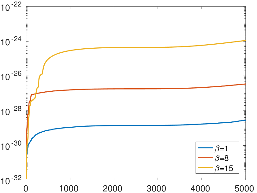
(a)

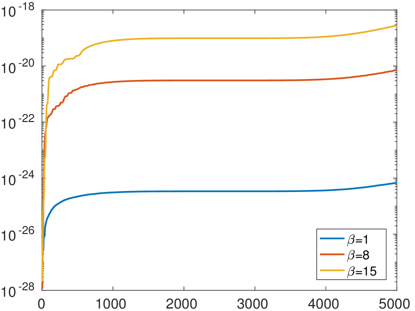
(b)

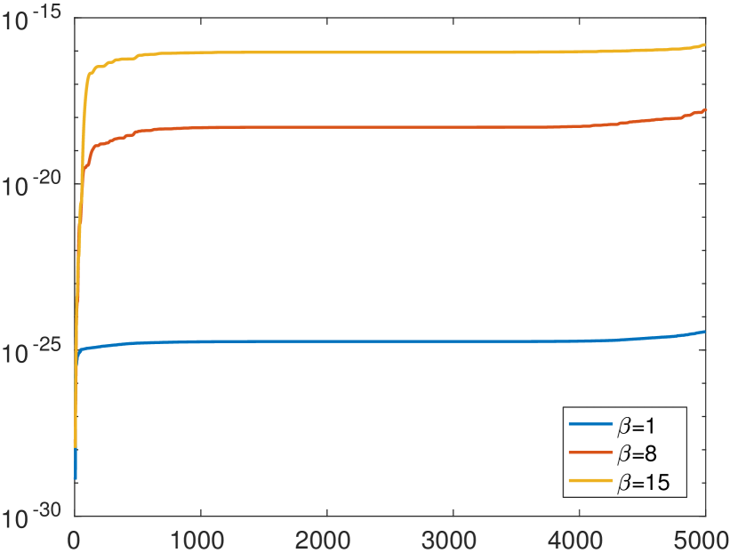
(c)

Figure 3: Approximation errors $\mathcal{E}^{{1:r}},$ $r=1,...,N,$ for (a) a linear polynomial and order $k=2,$ for (b) a quadratic polynomial and order $k=3,$ and for (c) a cubic polynomial and order $k=4.$ The theoretical approximation errors are equal to zero; the approximation errors computed using the recurrence formula (37) are accurate up to machine precision.

Next we explain how to include the two pruning strategies from Section 3.1. The first strategy with condition (26) requires to run over the $l$-index in a descending way, i.e. in the order $l=r,r-1,\ldots,1$. On the other hand, the second strategy demands checking (27) for all $1<l<r$ after $P_{r}^{*}$ was determined. Consequently, if (26) holds for some $l$ at $(1:r)$, condition (27) cannot be checked for $l^{\prime}<l$ since $\mathcal{E}^{l^{\prime}:r}$ has not been computed yet. In order to overcome this issue without obliterating the first pruning, we proceed as follows. At domain $(1:r)$, run through all $l$ in the descending list $L$ and update successively the corresponding approximation errors to $\mathcal{E}^{{l:r}}$. After each update step, check whether (27) is satisfied for the current upper interval bound of the error and if so, delete $l$ from $L$ and start again with the next entry in $L$. By this, it is not necessary to adapt the second pruning strategy essentially: check condition (26) after testing if a not pruned $l$ is the current optimal last changepoint. By combining the pruning strategies we effectively decrease the total number of error updates (37) that have to be performed; see Section 4.2 for a numerical study.

We provide a pseudocode for the proposed solver in the appendix (Algorithm 1). Let us summarize the above derivation:

Theorem 6.

Let $f\in\mathbb{R}^{N},$ $k\in\mathbb{N},$ and $\beta,\gamma>0.$ The proposed algorithm computes a global minimizer of ($\mathcal{P}_{k,\beta,\gamma}$). The worst case time complexity is $\mathcal{O}(N^{2}).$

Proof.

It follows from the Bellman equation (25) that the algorithm computes indeed a global minimizer. The double loop over the the $l$ and $r$ indices has quadratic worst-case complexity. It remains to show that for each $r\in(1:N)$ we can compute $\mathcal{E}^{{r-k:r}},$ $\mathcal{E}^{{r-k-1:r}},$ …, $\mathcal{E}^{{1:r}}$ in $O(1)$ per element. As each line of $A$ has at most $k+1$ entries, the elimination of one line requires $k+1$ elimination steps. By the band structure of $A$ each elimination step by Givens rotations creates only new non-zeros in a band of $k+1$ entries above the diagonal $A_{ii},$ $i=1,\ldots,N.$ Thus, computing the recurrence coefficients needs only $\mathcal{O}(k^{2}N)$ operations. As applying a Givens rotation to a vector only needs a constant amount of operations, the multiplication in (34) is in $O(k).$ (Note that the matrix $G^{(r+1)}$ is not explicitly created.) Hence, executing the recurrence (37) is $\mathcal{O}(k).$ It follows that computing the errors for all $\mathcal{O}(N^{2})$ intervals sums up to $\mathcal{O}(kN^{2}).$ The reconstruction step from a partition is in $\mathcal{O}(kN)$ as it reduces to solving a least squares system of band matrices whose number of rows sum up at most $2N-k.$ As $k$ is fixed the overall worst case time complexity is $\mathcal{O}(N^{2}).$ ∎

3.3 Fast computation of the approximation errors for higher order Potts problems

We describe a stable yet fast procedure to compute the approximation errors for the higher order Potts problems (14). To this end, we first rewrite (14) in terms of the polynomial coefficients $p\in\mathbb{R}^{k}$ as

$$\mathcal{E}^{l:r}=\min_{p\in\mathbb{R}^{k}}\|B_{l:r,1:r}p-f_{l:r}\|_{2}^{2},$$ (38)

where $B$ is the $\mathbb{R}^{N\times k}$ matrix defined by

$$B=\begin{pmatrix}1&1&\cdots&1^{k-1}\\ 1&2&\cdots&2^{k-1}\\ \vdots&\vdots&&\vdots\\ 1&N-1&\cdots&(N-1)^{k-1}\\ 1&N&\cdots&N^{k-1}\end{pmatrix}\in\mathbb{R}^{N\times k}.$$ (39)

As in Section 3.2, we describe the method for the prototypical case $l=1.$ Furthermore, we assume that $r>k$ since otherwise $\mathcal{E}^{{1:r}}=0$. Denoting the submatrix $B_{1:r,1:k}$ by $B^{(r)}$ and its QR decomposition by $Q^{(r)},R^{(r)},$ we obtain in analogy to (31) that

$$\begin{split}\mathcal{E}^{{1:r}}&=\min_{p\in\mathbb{R}^{k}}\bigg{\|}\begin{pmatrix}R^{(r)}\\ 0\end{pmatrix}p-(Q^{(r)})^{T}f_{1:r}\bigg{\|}_{2}^{2}=\|q^{(r)}_{k+1:r}\|_{2}^{2},\end{split}$$ (40)

where $q^{(r)}$ is given by

$$q^{(r)}=(Q^{(r)})^{T}f_{1:r}.$$

The recurrence coefficients for the error update $\Theta_{r+1,j}$ for $j=1,\ldots,k$ are the Givens rotation angles for eliminating the entry $B_{r+1,j}$ with the pivot element $R^{(r)}_{j,j}.$ Now assume that we have computed $q^{(r)}$ and $\mathcal{E}^{{1:r}}.$ Then, $q^{(r+1)}$ can be expressed by the recurrence relation

$$q^{(r+1)}=G^{(r+1)}\begin{pmatrix}q^{(r)}\\ f_{r+1}\end{pmatrix},$$ (41)

where $G^{(r+1)}$ comprises the Givens rotations $G(j,r+1,\Theta_{r+1,j})$ for $j=1,\ldots,k;$ that is,

$$G^{(r+1)}=\prod_{j=1}^{k}G(j,r+1,\Theta_{r+1,j}),$$ (42)

where we again use the convention $\prod_{j=1}^{k}Z_{j}=Z_{k}Z_{k-1}\cdots Z_{1}$. As $G^{(r+1)}$ operates only on the first $k$ entries and the last entry of $q^{(k)},$ we obtain by (40)

$$\begin{split}\mathcal{E}^{{1:r+1}}=\|q^{(r+1)}_{k+1:r+1}\|_{2}^{2}=\|q^{(r)}_{k+1:r}\|_{2}^{2}+(q^{(r+1)})_{r+1}^{2}=\mathcal{E}^{{1:r}}+(q^{(r+1)})_{r+1}^{2}\end{split}.$$ (43)

Remark 7.

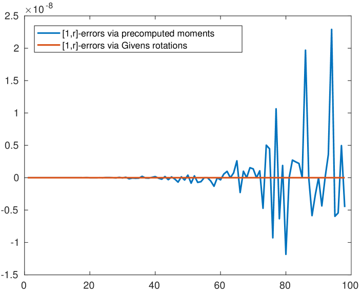
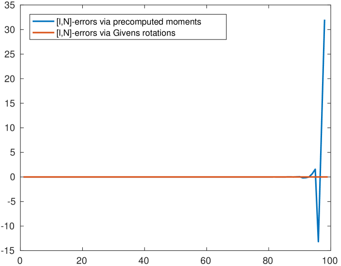
Figure 4: Approximation errors for a parabolic signal for the higher order Potts model of order $k=3.$ The graphs show the results based on precomputed moments (blue) and based on the proposed scheme (red). The true approximation errors are all equal to zero. Left:  Errors $\mathcal{E}^{1:r}$ for $r=1,...,N$. The computation based on precomputed moments is distorted beyond machine precision and gives even negative values. Right: Errors $\mathcal{E}^{l:N}$ for $l=1,...,N-1$. The values derived from precomputed moments are strongly distorted when $l$ approaches $N.$ The proposed computation based on Givens rotations is accurate up to machine precision in either case.

For the higher order Potts problems, there are also closed formulae for the evaluation of the errors $\mathcal{E}^{l:r}$ which one might consider to use directly. Such formulae are derived in [26] and in [41] for the first and the second order Potts problem, respectively. Using computer algebra, we have derived such formulae for $k=3$ and $k=4.$ By precomputing moments, the errors $\mathcal{E}^{l:r}$ can then be computed in $\mathcal{O}(1)$ per element. The results are typically acceptable for the piecewise constant and piecewise affine linear problems ($k=1,2$) and moderate signal lengths. Unfortunately, for higher orders or longer signals, the approach based on the precomputation of moments is prone to numerical instability. This is illustrated by the following experiment (cf. Figure 4). We consider the parabolic signal $f_{n}=n^{2}/100$, $n=0,...,N$ where $N=100.$ The true approximation errors for the higher order Potts model of order $k=3$ are given by $\mathcal{E}^{l:r}=0$ for all $l,r$ with $1\leq l\leq r\leq N.$ Figure 4 shows that the results for $\mathcal{E}^{1:r}$ are distorted when using the approach based on the precomputation of moments, in particular if $r$ is close to $N.$ The errors $\mathcal{E}^{l:N}$ are even more severely affected because of loss of significance. We observe that – in contrast to the moment precomputation approach – the proposed method gives accurate results up to machine precision.

3.4 Stability results

In this section, we investigate the stability of the proposed algorithm. We start out with some basic lemmas we will need later on. In the following, we consider the functional $\mathcal{G}_{[\mathcal{I}]}(f)$ defined in (19) and omit the brackets and simply write $\mathcal{G}_{\mathcal{I}}(f).$

Lemma 8.

We consider data $f\in\mathbb{R}^{N}.$ If there is a partition $\mathcal{I}^{\prime}$ and $\varepsilon>0$ such that

$$\mathcal{G}_{\mathcal{I}^{\prime}}(f)<\mathcal{G}_{\mathcal{I}}(f)-\varepsilon\quad\text{ for all }\quad\mathcal{I}\notin[\mathcal{I}^{\prime}]$$ (44)

then there is an euclidean $\delta$-ball $B(f,\delta)$ around $f$ such that for any $g\in B(f,\delta)$ holds: for data $g$ there is a unique optimal solution $u=u_{g,\mathcal{I}^{*}}$ of the problem ($\mathcal{P}_{k,\beta,\gamma}$), and the corresponding partition $\mathcal{I}^{*}$ fulfills $[\mathcal{I}^{*}]=[\mathcal{I}^{\prime}].$ We may choose $\delta$ by

$$\delta:=\min\left(\frac{\varepsilon}{2(2\beta)^{2k}\ (\|f\|+1/2)},\frac{1}{2}\right).$$ (45)

Proof.

The essential argument here relies on the continuity of the quadratic forms $x\mapsto\bar{\mathcal{G}}_{\mathcal{I}}(x)$ given by

$$\bar{\mathcal{G}}_{\mathcal{I}}(f):=\beta^{2k}\,\|L_{\mathcal{I}}S_{\mathcal{I}}f\|_{2}^{2}+\|S_{\mathcal{I}}f-f\|_{2}^{2}$$ (46)

which are the main parts of the $\mathcal{G}_{\mathcal{I}}$ given by (19). Each $\bar{\mathcal{G}}_{\mathcal{I}}$ may be represented w.r.t. the euclidean standard scalar product $\langle\cdot,\cdot\rangle$ via a symmetric matrix $A_{\mathcal{I}}$ as $\bar{\mathcal{G}}_{\mathcal{I}}(x)=\langle A_{\mathcal{I}}x,x\rangle.$ The operator norm of $A_{\mathcal{I}}$ equals the norm of the corresponding bilinear form which in turn, since the $\bar{\mathcal{G}}_{\mathcal{I}}$ are positive (semi-definite), corresponds to

$$\|A_{\mathcal{I}}\|=\sup_{x:\|x\|=1}\bar{\mathcal{G}}_{\mathcal{I}}(x).$$ (47)

We first let $\delta^{\prime}$ be defined by

$$\delta^{\prime}:=\min\left(\frac{1}{2},\frac{\varepsilon}{2\max_{\mathcal{I}}\|A_{\mathcal{I}}\|\ (\|f\|+1/2)}\right).$$ (48)

We want to estimate $\mathcal{G}_{\mathcal{I}^{\prime}}(f)$ from above for $g$ in a $\delta^{\prime}$-ball around $f.$ For brevity, we write $\mathcal{G}_{\mathcal{I}^{\prime}}(g)=\bar{\mathcal{G}}_{\mathcal{I}^{\prime}}(g)+\gamma N_{\mathcal{I}^{\prime}}$ where we let $N_{\mathcal{I}^{\prime}}:=|[\mathcal{I}^{\prime}]|$. Then we may estimate

$$\mathcal{G}_{\mathcal{I}^{\prime}}(g)=\bar{\mathcal{G}}_{\mathcal{I}^{\prime}}(g)+\gamma|[\mathcal{I}^{\prime}]| =\bar{\mathcal{G}}_{\mathcal{I}^{\prime}}(f)+\bar{\mathcal{G}}_{\mathcal{I}^{\prime}}(f-g)-2\langle A_{\mathcal{I}}^{\prime}f,f-g\rangle+\gamma|[\mathcal{I}^{\prime}]|$$

$$<\bar{\mathcal{G}}_{\mathcal{I}}(f)-\varepsilon+\delta^{\prime 2}\ \|A_{\mathcal{I}^{\prime}}\|+\delta^{\prime}\ \|A_{\mathcal{I}^{\prime}}\|\ \|f\|+\gamma|[\mathcal{I}]|$$

$$=\bar{\mathcal{G}}_{\mathcal{I}}(g)+\bar{\mathcal{G}}_{\mathcal{I}}(f-g)+2\langle A_{\mathcal{I}}f,f-g\rangle-\varepsilon+\delta^{\prime 2}\ \|A_{\mathcal{I}^{\prime}}\|+\delta^{\prime}\ \|A_{\mathcal{I}^{\prime}}\|\ \|f\|+\gamma|[\mathcal{I}]|$$

$$\leq\bar{\mathcal{G}}_{\mathcal{I}}(g)-\varepsilon+2\delta^{\prime}\ \max_{\mathcal{I}}\|A_{\mathcal{I}}\|\ \ (\|f\|+\delta^{\prime})+\gamma|[\mathcal{I}]|$$

$$\leq\bar{\mathcal{G}}_{\mathcal{I}}(g)-\varepsilon+\varepsilon+\gamma|[\mathcal{I}]|=\bar{\mathcal{G}}_{\mathcal{I}}(g)+\gamma|[\mathcal{I}]|=\mathcal{G}_{\mathcal{I}}(g).$$ (49)

For the first inequality, we applied (44) for $\mathcal{G}_{\mathcal{I}^{\prime}}(f)$ and used the assumption that $g\in B(f,\delta^{\prime}).$ For the second inequality, we employed (48). In order to relate (48) with (45), we now estimate $\max_{\mathcal{I}}\|A_{\mathcal{I}}\|$ using basic spectral theory for self-adjoint bounded operators. Since $A_{\mathcal{I}}$ is the matrix representing the bilinear form corresponding to $\bar{\mathcal{G}}_{\mathcal{I}},$ we may estimate using (46) that

$$\|A_{\mathcal{I}}\|\leq\beta^{2k}\|L_{\mathcal{I}}^{T}L_{\mathcal{I}}\|\ \|S_{\mathcal{I}}\|^{2}+\|I-S_{\mathcal{I}}\|^{2},\quad\text{ for any partition }\mathcal{I},$$ (50)

with the definitions of $L_{\mathcal{I}}$ given in (9) and that of $S_{\mathcal{I}}$ given in (12); here we only employed the triangle inequality and the submultiplicativity of operator norms. By (12), $S_{\mathcal{I}}=$ $(\beta^{2k}L_{\mathcal{I}}^{T}L_{\mathcal{I}}+\mathrm{id})^{-1}.$ Since $L_{\mathcal{I}}^{T}L_{\mathcal{I}}$ is self-adjoint and positive, the spectrum of $\beta^{2k}L_{\mathcal{I}}^{T}L_{\mathcal{I}}+\mathrm{id}$ is contained in $[1,\infty).$ Hence, its inverse $S_{\mathcal{I}}$ has its spectrum contained in $[0,1].$ Being again self-adjoint, and positive, $\|S_{\mathcal{I}}\|\leq 1.$ Further, since $S_{\mathcal{I}}$ has its spectrum contained in $[0,1],$ $I-S_{\mathcal{I}}$ has its spectrum contained in $[0,1]$ as well. Then, with the same argument, $\|I-S_{\mathcal{I}}\|\leq 1.$ In order to estimate $L_{\mathcal{I}}^{T}L_{\mathcal{I}},$ we consider $L_{\mathcal{I}}$ in (9), and notice that $L_{\mathcal{I}}^{T}L_{\mathcal{I}}$ is block diagonal with entries consisting of convolutions of $k$th differences with themselves. Thus the row-sums as well as the column sums of $L_{\mathcal{I}}^{T}L_{\mathcal{I}}$ are bounded by $2^{2k}.$ The using the Schur criterion, the operator norm of $L_{\mathcal{I}}^{T}L_{\mathcal{I}}$ w.r.t. euclidean norm in the base space can be estimated by $2^{2k}.$ Summing up, we conclude invoking these estimates in (50) that

$$\|A_{\mathcal{I}}\|\leq\beta^{2k}2^{2k}+1,\quad\text{ for any partition }\mathcal{I}.$$ (51)

We now can show the assertion of the lemma. If $g\in B(f,\delta),$ then $g\in B(f,\delta^{\prime}),$ by the estimate (51) relating (48) with (45). In consequence, the estimate (49) applies to $g.$ Hence the solution for $g$ is unique and given by (12); in particular, the corresponding equivalence class of partitions equals $\mathcal{I}^{\prime}$ which shows the assertion. ∎

Next, we need a backward stability result for the QR algorithm [28]. We present it adapted to our setup as needed later on. In analogy to (12), we denote the linear mapping from $f_{I}$ (restricted to the interval $I$) to the solution $u_{I}$ by $S_{I}.$

Theorem 9.

The QR algorithm $\tilde{S}_{{l:r}}$ needed for computing the $\mathcal{E}^{{l:r}}$ is backward stable, i.e., given data $f_{{l:r}}$ living on the subinterval ${l:r},$ there is a perturbation $\tilde{f}_{{l:r}}$ of $f_{{l:r}}$ such that

$$\tilde{S}_{{l:r}}(f_{{l:r}})=S_{{l:r}}(\tilde{f}_{{l:r}})\quad\text{ with }\quad\|\tilde{f}_{{l:r}}-f_{{l:r}}\|\leq\delta_{{l:r}},$$ (52)

where $\delta_{{l:r}}$ depends on the machine precision $\tau$ and on the norm $\|f_{{l:r}}\|$ via

$$\delta_{{l:r}}\leq 6\tau\sqrt{r-l+1}\cdot\left(\frac{9(r-l+1)-5}{4}-k\right)(1+6\tau)^{3(r-l)-k}\|f_{{l:r}}\|.$$ (53)

Here, the QR algorithm is understood as in the analysis setup of [28, 71].

Proof.

If $r-l<k,$ then $\tilde{S}_{{l:r}}(f_{{l:r}})=S_{{l:r}}(f_{{l:r}})=0$. So we may assume $r-l\geq k$. Recall that calculating $\mathcal{E}^{{l:r}}$ corresponds to computing the residual vector of the least squares problem with system matrix $A\in\mathbb{R}^{2(r-l+1)-k\times(r-l+1)}$ from (29) and data $f_{{l:r}}$. In [28] it is shown that

$$\tilde{R}=\bar{Q}^{T}(A+\Delta A),\quad\|\Delta A\|_{F}\leq\mu_{{l:r}}(\tau)\|A\|_{F},$$

$$\mu_{{l:r}}(\tau)=6\tau\sqrt{r-l+1}\cdot\left(\frac{9(r-l+1)-5}{4}-k\right)(1+6\tau)^{3(r-l)-k},$$

where $\tilde{R}$ is the computed upper triangular matrix by means of Givens rotations and note that $\bar{Q}^{T}$ is the orthogonal matrix that is the product of exact Givens rotations we apply. Analogously, for the data vector it is shown in [28] that

$$\widetilde{Q^{T}f_{{l:r}}}=\bar{Q}^{T}(f_{{l:r}}+\Delta f_{{l:r}}),\quad\|\Delta f_{{l:r}}\|\leq\mu_{{l:r}}(\tau)\|f_{{l:r}}\|,$$

hence $\tilde{S}_{{l:r}}(f_{{l:r}})=S_{{l:r}}(f_{{l:r}}+\Delta f_{{l:r}})$ which implies (53). ∎

Corollary 10.

We consider bounded data $f\in\mathbb{R}^{N},$ $\|f\|<C.$ For any partition $\mathcal{I}$ considered in the proposed algorithm for the higher order Potts and Mumford-Shah problem, there is a perturbation $\tilde{f}$ of $f$ such that

$$\tilde{S}_{\mathcal{I}}(f)=S_{\mathcal{I}}(\tilde{f})\quad\text{ where }\quad\|\tilde{f}-f\|<\delta_{\mathcal{I}}(\tau),$$ (54)

where $\delta_{\mathcal{I}}(\tau)^{2}=\sum_{i}\delta_{l_{i}:r_{i}}(\tau)^{2}$ depends on the machine precision $\tau$ via the dependence of the $\delta_{l_{i}:r_{i}}$ on $\tau$ given in Theorem 9 and on $C,$ but not on $f.$ More precisely, $\delta_{\mathcal{I}}(\tau)$ can be estimated from above by

$$\delta_{\mathcal{I}}(\tau)^{2}\leq 36C^{2}\tau^{2}\sum_{i}(r_{i}-l_{i}+1)\left(\frac{9(r_{i}-l_{i}+1)-5}{4}-k\right)^{2}(1+6\tau)^{6(r-l)-2k}.$$ (55)

Proof.

The statement is a consequence of Theorem 9 since, for fixed partition, the proposed algorithm computes optimal solutions $u_{f,\mathcal{I}}=S_{\mathcal{I},\beta}f$ (cf. (12)) using the QR algorithm on intervals. In particular, (55) is a consequence of (53). ∎

For the formulation of the next statement, we use the notation $\tilde{\mathcal{G}}_{\mathcal{I}}$ to denote the algorithm to compute the energy $\mathcal{G}_{\mathcal{I}}$ given by (19). Further, we use the notation $g(\tau)$ to bound the approximation error between $\tilde{\mathcal{G}}_{\mathcal{I}}$ and $\mathcal{G}_{\mathcal{I}}$ for all $\mathcal{I}$ in dependence of the precision $\tau.$

Proposition 11.

We consider bounded data $f\in\mathbb{R}^{N},$ $\|f\|<C$, and assume that (44) is fulfilled for $f.$ Let

$$\delta^{*}(\tau)=\max_{\mathcal{I}}\delta_{\mathcal{I}}(\tau)\leq 6C\tau N^{\frac{3}{2}}\left(\frac{9N-5}{4}-k\right)(1+6\tau)^{3(N-1)-k}$$ (56)

for $\delta_{\mathcal{I}}(\tau)$ in Corollary 10 and assume that $\tau$ is small enough such that $\delta^{*}(\tau)<\delta/2$ with $\delta$ given by (45) and such that $g(\tau)\leq\varepsilon/4$ with $\varepsilon$ given in (44). Then, the higher order Potts and Mumford-Shah problem ($\mathcal{P}_{k,\beta,\gamma}$) has a unique minimizer $u_{f},$ and the proposed algorithm for computing this minimizer of the higher order Potts and Mumford-Shah problem ($\mathcal{P}_{k,\beta,\gamma}$) is backward stable in the sense that

$$\tilde{u}_{f}=u_{\tilde{f}}\quad\text{ where }\quad\|\tilde{f}-f\|<\delta^{*}(\tau).$$ (57)

Here, $\tilde{u}_{f}$ is the result produced by the proposed algorithm for data $f$ and $u_{\tilde{f}}$ is the (unique) solution of the higher order Potts and Mumford-Shah problem ($\mathcal{P}_{k,\beta,\gamma}$) for perturbed data $\tilde{f}.$

Remark 12.

A more explicit relation of $\varepsilon$ and the precision $\tau$ without using the $\delta$’s sufficient for the assumptions of Proposition 11 to hold is given by

$$(1+6\tau)^{3N-k}\tau <\frac{\varepsilon}{12CN(2\beta)^{2k}(C+\frac{1}{2})\left(\frac{9N-5}{4}-k\right)}\quad\text{if }\varepsilon\leq(2\beta)^{2k}(C+\frac{1}{2}),$$ (58)

$$(1+6\tau)^{3N-k}\tau <\frac{1}{12CN\left(\frac{9N-5}{4}-k\right)}\qquad\qquad\qquad~{}~{}\text{if }\varepsilon>(2\beta)^{2k}(C+\frac{1}{2}),$$ (59)

$$\mu_{[1,N]}(\tau) <\frac{1}{2}\left(\frac{4C^{2}N+\varepsilon}{C^{2}N}\right)^{\frac{1}{2}}-1$$ (60)

w.r.t. $\mu_{[1,N]}(\tau)$ from the proof of Theorem 9. Conditions (58) and (59) are sufficient for $\delta^{*}(\tau)<\delta/2$ which is an immediate implication of combining (44) and (56). From (60) follows $g(\tau)\leq\varepsilon/4$ since: for any admissible ${l:r}$ we have

$$\left\lvert\|\widetilde{Q^{T}f_{{l:r}}}\|^{2}-\|Q^{T}f_{{l:r}}\|^{2}\right\rvert \leq\left(\|Q^{T}f_{{l:r}}\|+\|\widetilde{Q^{T}f_{{l:r}}}\|\right)\left\lvert\|Q^{T}f_{{l:r}}\|-\|\widetilde{Q^{T}f_{{l:r}}}\|\right\rvert$$

$$\leq\left(C+\|\widetilde{Q^{T}f_{{l:r}}}\|\right)\|Q^{T}f_{{l:r}}-\widetilde{Q^{T}f_{{l:r}}}\|$$

and

$$\|\widetilde{Q^{T}f_{{l:r}}}\|\leq\|Q^{T}f_{{l:r}}\|+\|Q^{T}f_{{l:r}}-\widetilde{Q^{T}f_{{l:r}}}\|\leq C+\|Q^{T}f_{{l:r}}-\widetilde{Q^{T}f_{{l:r}}}\|\leq C+\mu_{[1,N]}C.$$

Combining both yields

$$g(\tau) =\left\lvert\tilde{\mathcal{G}}_{\mathcal{I}}(f)-\mathcal{G}_{\mathcal{I}}(f)\right\rvert\leq\sum_{{l:r}\in\mathcal{I}}\left\lvert\tilde{\mathcal{E}}^{{l:r}}-\mathcal{E}^{{l:r}}\right\rvert$$

$$\leq\sum_{{l:r}\in\mathcal{I}}\left\lvert\|\widetilde{Q^{T}f_{{l:r}}}\|^{2}-\|Q^{T}f_{{l:r}}\|^{2}\right\rvert\leq NC^{2}\mu_{[1,N]}(\tau)\left(2+\mu_{[1,N]}(\tau)\right).$$

An easy computation shows that (60) is equivalent to requiring the latter to be smaller than $\varepsilon/4$.

Proof of Proposition 11.

By the proof of Theorem 5, the solution $u_{f}$ of ($\mathcal{P}_{k,\beta,\gamma}$) is unique for data $f.$ We denote the equivalence class of partitions corresponding to this optimal solution $u_{f}$ by its representer $\mathcal{I}^{\prime}.$ As a first step, we show that the solution $\tilde{u}_{f}$ computed by the proposed algorithm for data $f$ has partition $\mathcal{I}^{\prime}$ as well. To that end, we first notice that by Corollary 10, there is $\tilde{f}_{\mathcal{I}}$ with $\|\tilde{f}_{\mathcal{I}}-f\|<\delta_{\mathcal{I}}(\tau)$ such that $\tilde{S}_{\mathcal{I}}(f)=S_{\mathcal{I}}(\tilde{f}_{\mathcal{I}}),$ for any partition $\mathcal{I}$ which is considered by the algorithm. In particular, using the notation of Theorem 9,

$$\|\tilde{S}_{{l:r}}(f_{{l:r}})-S_{{l:r}}(f_{{l:r}})\| =\|S_{{l:r}}(\tilde{f}_{{l:r}})-S_{{l:r}}(f_{{l:r}})\|$$

$$\leq\|S_{{l:r}}\|\ \|\tilde{f}_{{l:r}}-f_{{l:r}}\|\leq\|\tilde{f}_{{l:r}}-f_{{l:r}}\|<\delta_{{l:r}}.$$ (61)

For the second before last inequality, we used that $\|S_{{l:r}}\|\leq 1$ which we have shown in the proof of Lemma 8. In consequence, summing over all intervals of $\mathcal{I}$ of length at least $k+1,$ we obtain from (61) that

$$\|\tilde{S}_{\mathcal{I}}(f)-S_{\mathcal{I}}(f)\|=\|S_{\mathcal{I}}(\tilde{f}_{\mathcal{I}})-S_{\mathcal{I}}(f)\|\leq\|\tilde{f}_{\mathcal{I}}-f\|<\delta_{\mathcal{I}}(\tau).$$ (62)

for any partition $\mathcal{I}$ which is considered by the algorithm. Then, using the notation $\tilde{\mathcal{G}}_{\mathcal{I}}$ for the algorithmic variant of $\mathcal{G}_{\mathcal{I}},$ we have (with the notation as in Lemma 8) that

$$\tilde{\mathcal{G}}_{\mathcal{I}^{\prime}}(\tilde{f}_{\mathcal{I}^{\prime}}) \leq\mathcal{G}_{\mathcal{I}^{\prime}}(\tilde{f}_{\mathcal{I}^{\prime}})+|\tilde{\mathcal{G}}_{\mathcal{I}^{\prime}}(\tilde{f}_{\mathcal{I}^{\prime}})-\mathcal{G}_{\mathcal{I}^{\prime}}(\tilde{f}_{\mathcal{I}^{\prime}})|$$

$$\leq\mathcal{G}_{\mathcal{I}^{\prime}}(\tilde{f}_{\mathcal{I}^{\prime}})+g(\tau)$$

$$<\mathcal{G}_{\mathcal{I}}(f)-\varepsilon+\delta_{\mathcal{I}^{\prime}}(\tau)^{2}\ \|A_{\mathcal{I}^{\prime}}\|+\delta_{\mathcal{I}^{\prime}}(\tau)\ \|A_{\mathcal{I}^{\prime}}\|\ \|f\|+g(\tau)$$

$$\leq\mathcal{G}_{\mathcal{I}}(\tilde{f}_{\mathcal{I}})-\varepsilon+2\delta^{\ast}(\tau)\ \max_{\mathcal{I}}\|A_{\mathcal{I}}\|\ \ (\|f\|+\delta^{\ast}(\tau))+g(\tau)$$

$$\leq\mathcal{G}_{\mathcal{I}}(\tilde{f}_{\mathcal{I}})-\varepsilon+\varepsilon/2+g(\tau)$$

$$\leq\tilde{\mathcal{G}}_{\mathcal{I}}(\tilde{f}_{\mathcal{I}})-\varepsilon+\varepsilon/2+2g(\tau)\leq\tilde{\mathcal{G}}_{\mathcal{I}}(\tilde{f}_{\mathcal{I}}).$$ (63)

Here, the third inequality is the central estimate which is obtained in analogy to the first part of the computation in (49) replacing the role of the vector $g$ there (not to be confused with $g(\tau)$) by that of the perturbation $\tilde{f}_{\mathcal{I}}^{\prime}$ of $f$ here. The fourth inequality is obtained in analogy to the second part of the computation in (49) with the role of the vector $g$ there replaced by the perturbation $\tilde{f}_{\mathcal{I}}$ of $f.$ The second before last and last inequality follow by our assumptions made on $\tau.$ Together, (63) tells us that the solution $\tilde{u}_{f}$ computed by the proposed algorithm has partition $\mathcal{I}^{\prime}$ and

$$\tilde{u}_{f}=\tilde{S}_{\mathcal{I}^{\prime}}(f).$$ (64)

Using again Corollary 10, we have

$$\tilde{S}_{\mathcal{I}^{\prime}}(f)=S_{\mathcal{I}^{\prime}}(\tilde{f})\quad\text{ for }\quad\|\tilde{f}-f\|<\delta_{\mathcal{I}^{\prime}}(\tau)\leq\delta^{*}(\tau),$$ (65)

with the perturbation $\tilde{f}$ of $f.$ We have that $\|\tilde{f}-f\|<\delta^{*}(\tau)<\delta$ with $\delta$ defined by (45). Therefore, we may now employ Lemma 8 to conclude that the solution of the higher order Potts and Mumford-Shah problem ($\mathcal{P}_{k,\beta,\gamma}$) denoted by $u_{\tilde{f}}$ agrees with the optimal solution for the partition $\mathcal{I}^{\prime}$ which we have denoted by $u_{\tilde{f},\mathcal{I}^{\prime}}=S_{\mathcal{I}}(\tilde{f}),$ i.e.,

$$u_{\tilde{f}}=u_{\tilde{f},\mathcal{I}^{\prime}}=S_{\mathcal{I}^{\prime}}(\tilde{f}).$$ (66)

Combined with (64) and (65), this shows (57) which completes the proof. ∎

Lemma 13.

We consider a nonzero quadratic form $H$ in a ball of radius $C$ in $\mathbb{R}^{N}$. Then, the Lebesgue measure $\lambda$ of the set $H_{\varepsilon,c}=\{x:\|x\|\leq C,c-\varepsilon<H(x)<c+\varepsilon\}$ fulfills

$$\lambda(H_{\varepsilon,c})\leq 2\sqrt{\frac{\varepsilon}{\|A\|}}\ C^{N-1}$$ (67)

where $\|A\|$ denotes the spectral norm of the representing matrix $A$ of $H.$

Proof.

Without loss of generality, we may use a orthogonal transformation of the coordinate system to represent $H$ by $H(x)=\sum_{i}\alpha_{i}x_{i}^{2}$ with the eigenvalues $\alpha_{i}$ of the corresponding representing matrix of the quadratic form. We sort the $\alpha_{i}$ by modulus, i.e., $|\alpha_{1}|\geq|\alpha_{2}|\geq\ldots.$ With repect to this coordinate system, we consider the $C$-ball with respect to the infinity norm $D=\{x:\|x\|_{\infty}\leq C\}$. We distinguish the eigenvalue $\alpha_{1}$ of highest modulus which agrees with the norm $\|A\|$ of the representing matrix $A$ of $H.$ We estimate the Lebesgue measure of $\{x:c-\varepsilon<H(x)<c+\varepsilon\}$ on the larger set $D$ which provides an upper bound for that of $H_{\varepsilon,c}.$ To this end, we notice that, for fixed $x_{2},\ldots,x_{N},$ we may estimate the univariate Lebesgue measure $\lambda^{1}$ of the section $\{x_{1}:\leq C,c-\varepsilon<H(x_{1},x_{2},\ldots,x_{N})<c+\varepsilon\}$

$$\lambda^{1}\left(c+\sum_{i=2}^{N}\frac{\alpha_{i}}{|\alpha_{1}|}x_{i}^{2}-\varepsilon<\operatorname{sign}(\alpha_{1})\ x_{1}^{2}<c+\sum_{i=2}^{N}\frac{\alpha_{i}}{|\alpha_{1}|}x_{i}^{2}+\varepsilon\right)\leq 2\sqrt{\frac{\varepsilon}{|\alpha_{1}|}}.$$ (68)

(Notice that if $\alpha_{1}=0$ the quadratic form would be zero.) Hence, on $D$, the Lebesgue measure of $\{x:c-\varepsilon<H(x)<c+\varepsilon\}$ is bounded by $2\sqrt{\frac{\varepsilon}{|\alpha_{1}|}}\ C^{N-1}$ which implies the assertion of the lemma. ∎

Theorem 14.

Let $\varepsilon>0$ be given and assume that the precision $\tau$ fulfills the assumptions of Proposition 11. We consider the set of bounded data $\{f:\|f\|\leq C\}$ in $\mathbb{R}^{N}$ for some $C>0.$ Then, up to a set of Lebesgue measure $2{\binom{\sigma_{N,k}}{2}}\sqrt{\frac{\varepsilon}{\sup_{\mathcal{I}}\|A_{\mathcal{I}}\|}}\ C^{N-1}$, $A_{\mathcal{I}}$ given by (47), $\sigma_{N,k}$ the number of different means to choose intervals of length at least $k+1$ from a (discrete) set of length $N,$ the proposed algorithm for computing a minimizer of the higher order Potts and Mumford-Shah problem ($\mathcal{P}_{k,\beta,\gamma}$) is backward stable in the sense that

$$\tilde{u}_{f}=u_{\tilde{f}}\quad\text{ where }\quad\|\tilde{f}-f\|<\delta^{*}(\tau),$$ (69)

where $\delta^{*}(\tau)$ is given by (56). Here, $\tilde{u}_{f}$ is the result produced by the proposed algorithm for data $f$ and $u_{\tilde{f}}$ is the (unique) solution of the higher order Potts and Mumford-Shah problem ($\mathcal{P}_{k,\beta,\gamma}$) for perturbed data $\tilde{f}.$

Proof.

We proceed similar to the proof of Theorem 5 to show that the set of those data which do not fulfill (44) have Lebesgue measure smaller or equal to $2{\binom{\sigma_{N,k}}{2}}\sqrt{\frac{\varepsilon}{\sup_{\mathcal{I}}\|A_{\mathcal{I}}\|}}\ C^{N-1}.$ We choose two different partitions $\mathcal{I},\mathcal{I}^{\prime}$ with $[\mathcal{I}]\neq[\mathcal{I}^{\prime}],$ i.e., their equivalence classes do not agree, and consider the corresponding quadratic forms $\mathcal{G}_{\mathcal{I}},\mathcal{G}_{\mathcal{I}^{\prime}}.$ Their difference $\mathcal{G}_{\mathcal{I}}-\mathcal{G}_{\mathcal{I}^{\prime}}$ is again a quadratic form (plus a constant). By Lemma 13, the set where $\mathcal{G}_{\mathcal{I}}$ and $\mathcal{G}_{\mathcal{I}^{\prime}}$ are closer than $\varepsilon$ has Lebesgue measure $2\sqrt{\frac{\varepsilon}{|\alpha_{1}|}}\ C^{N-1}.$ Iterating this for all ${\binom{\sigma_{N,k}}{2}}$ different bilinear forms $\mathcal{G}_{\mathcal{I}}-\mathcal{G}_{\mathcal{I}^{\prime}}$ shows that the Lebesgue measure of those data where (44) is not fulfilled can be estimated from above by the quantity written in the formulation of the theorem. To the complementary set, we may now apply Proposition 11 to conclude the assertion of the theorem. ∎

4 Numerical study

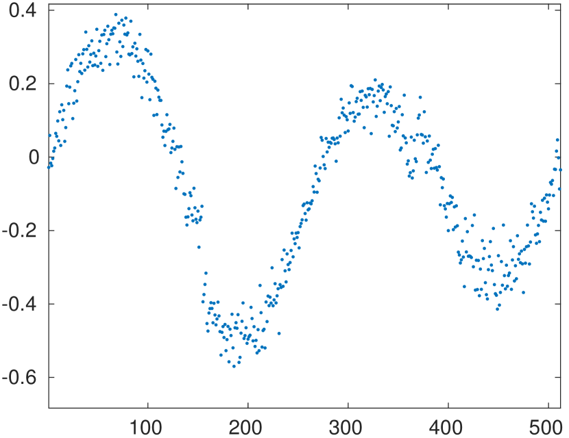
(a) Noisy data

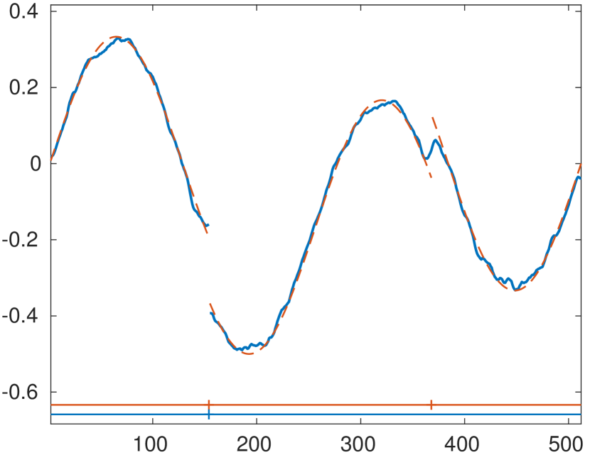
(b) $(\mathcal{P}_{1,\beta,\gamma})$, $\beta=4.050$, $\gamma=0.109$
$\varepsilon_{\text{rel}}=0.053$, $R_{\text{ind}}=0.76$

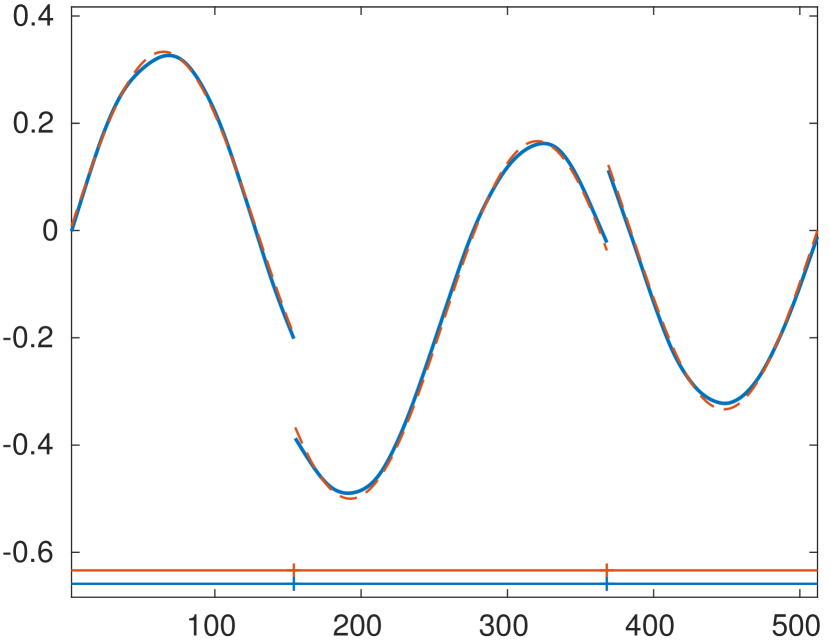
(c) $(\mathcal{P}_{2,\beta,\gamma})$, $\beta=9.500$, $\gamma=0.067$
$\varepsilon_{\text{rel}}=0.029$, $R_{\text{ind}}=1.00$

(d) $(\mathcal{P}_{3,\beta,\gamma})$, $\beta=12.850$, $\gamma=0.102$
$\varepsilon_{\text{rel}}=0.027$, $R_{\text{ind}}=1.00$

(e) $(\mathcal{P}_{4,\beta,\gamma})$, $\beta=15.300$, $\gamma=0.115$
$\varepsilon_{\text{rel}}=0.026$, $R_{\text{ind}}=1.00$

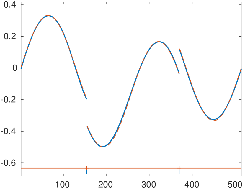
(f) $(\mathcal{P}_{5,\beta,\gamma})$, $\beta=18.850$, $\gamma=0.13$
$\varepsilon_{\text{rel}}=0.024$, $R_{\text{ind}}=1.00$

Figure 5: Reconstructions of “Heavy Sine”-signal from noisy data. (a) Data corrupted by Gaussian noise of level $0.2$. (b–f) Reconstructions for higher order Mumford-Shah and Potts models.

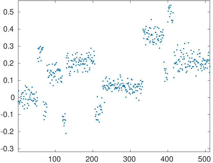
(a) Noisy data

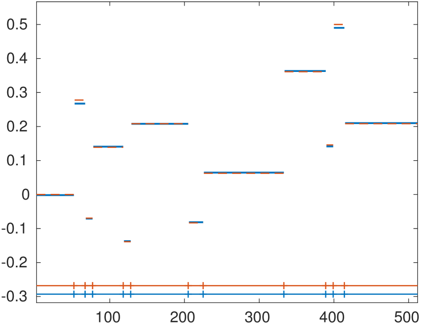
(b) $(\mathcal{P}_{1,\beta,\gamma})$, $\beta=\infty$, $\gamma=0.343$
$\varepsilon_{\text{rel}}=0.015$, $R_{\text{ind}}=1.00$

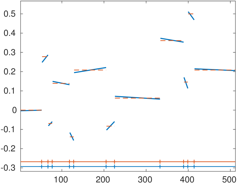
(c) $(\mathcal{P}_{2,\beta,\gamma})$, $\beta=\infty$, $\gamma=0.205$
$\varepsilon_{\text{rel}}=0.036$, $R_{\text{ind}}=1.00$

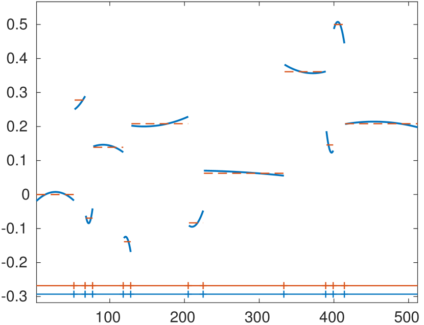
(d) $(\mathcal{P}_{3,\beta,\gamma})$, $\beta=\infty$, $\gamma=0.078$
$\varepsilon_{\text{rel}}=0.044$, $R_{\text{ind}}=1.00$

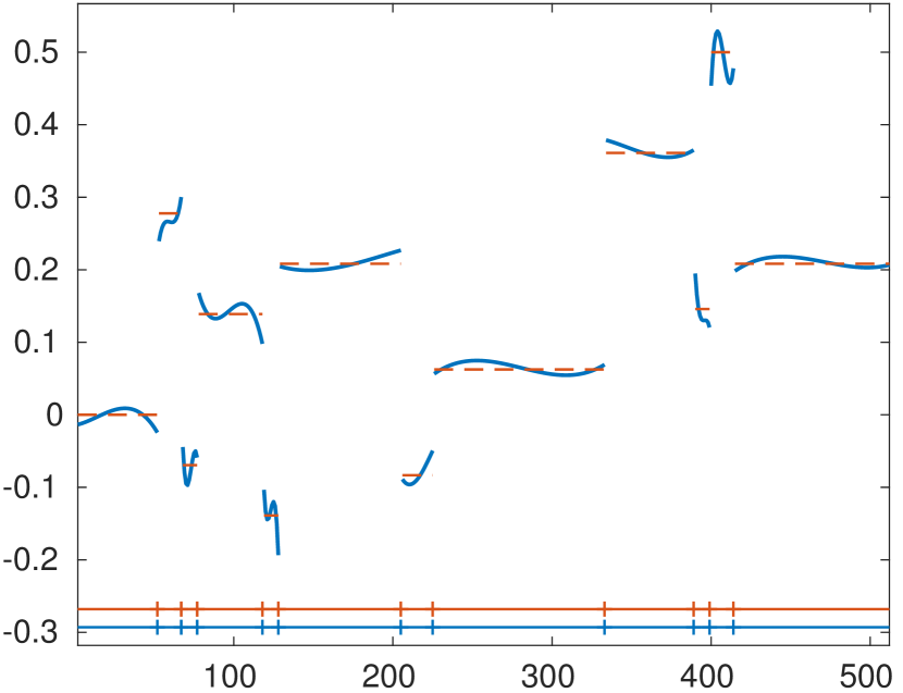
(e) $(\mathcal{P}_{4,\beta,\gamma})$, $\beta=\infty$, $\gamma=0.044$
$\varepsilon_{\text{rel}}=0.054$, $R_{\text{ind}}=1.00$

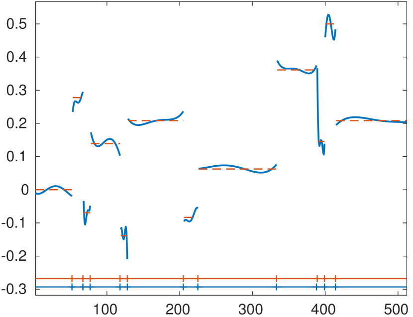
(f) $(\mathcal{P}_{5,\beta,\gamma})$, $\beta=24.300$, $\gamma=0.045$
$\varepsilon_{\text{rel}}=0.058$, $R_{\text{ind}}=0.99$

Figure 6: Reconstructions of “Blocks”-signal from noisy data. (a) Data corrupted by Gaussian noise of level $0.2$. (b–f) Reconstructions using higher order Mumford-Shah and Potts models.

We conduct a numerical study on the reconstruction quality of the considered higher order Mumford-Shah and Potts models, and on the computation time of the proposed solvers. We implemented the proposed solvers for the higher order Mumford-Shah and Potts models in C++ with wrappers to Matlab using mex-files. The pseudocode is given as Algorithm 1 in the appendix. All experiments were conducted on a desktop computer with 3.1 GHz Intel Core i5-2400 processor and 8 GB RAM.

4.1 Reconstruction results

(a) $\eta=0.05$

Noisy data
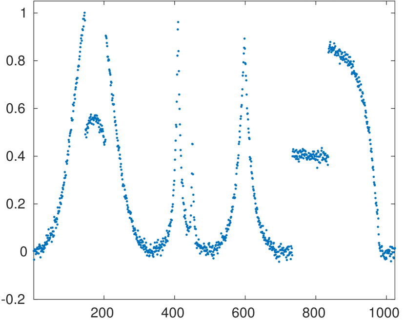
$k=1$
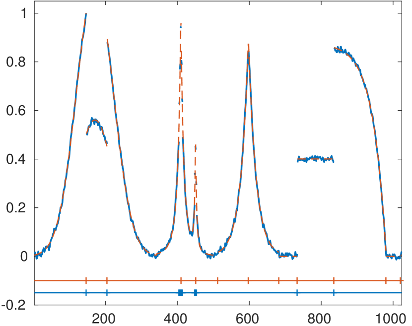
$k=2$
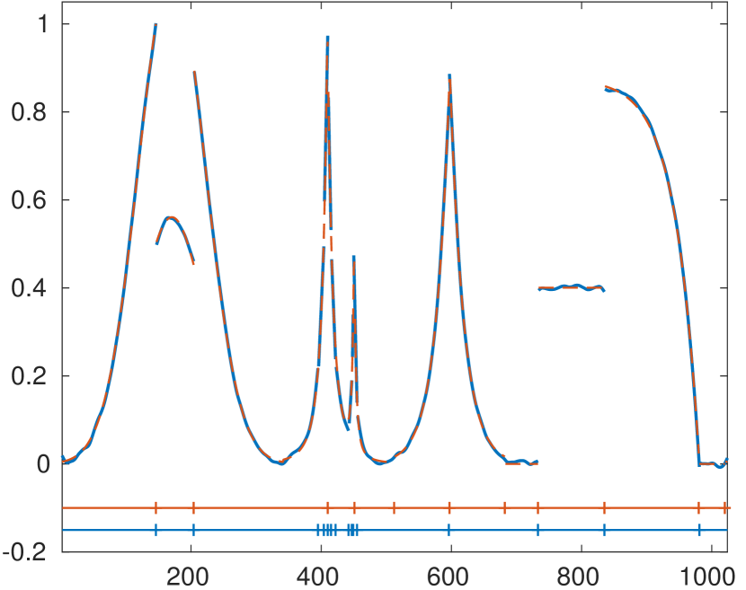
$k=3$
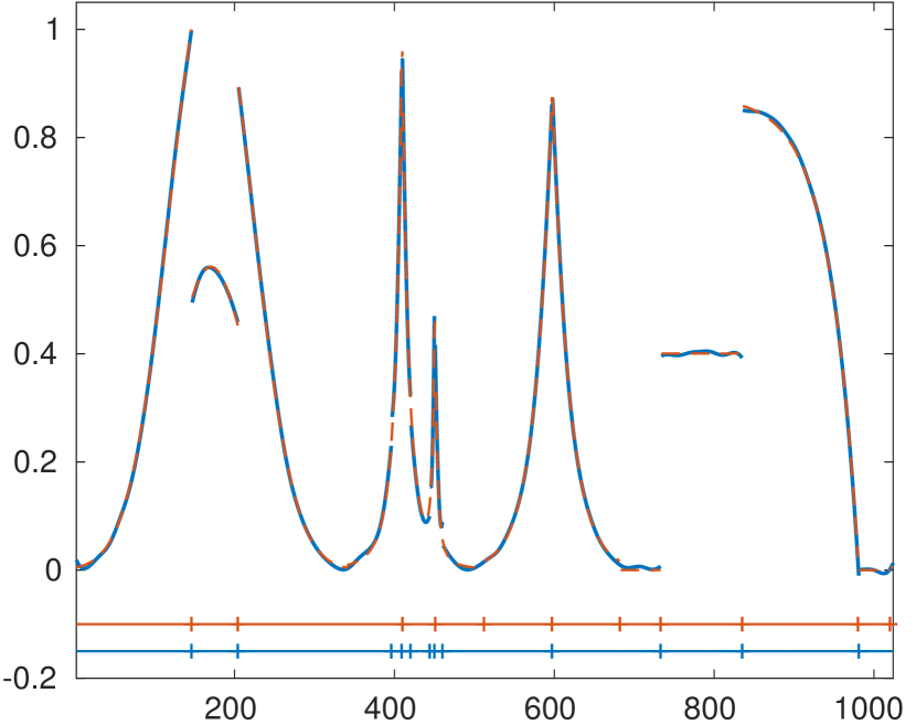
$k=4$

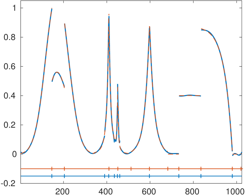
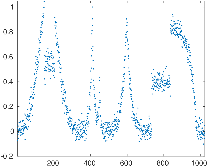
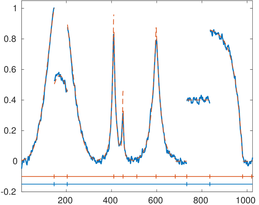
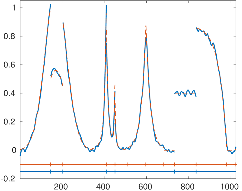
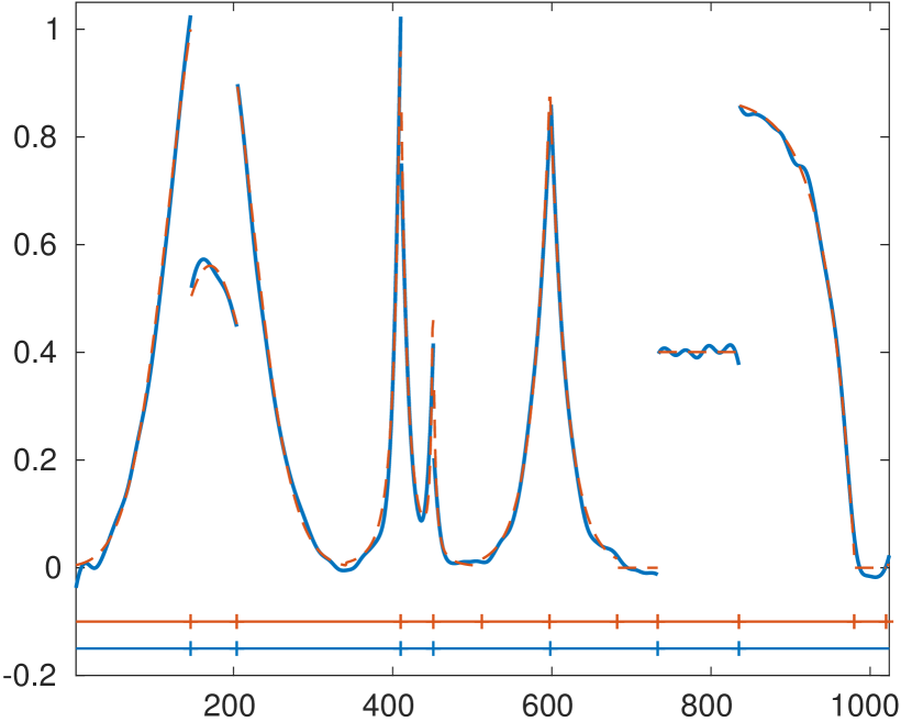
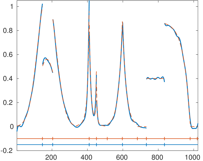
(b) $\eta=0.15$

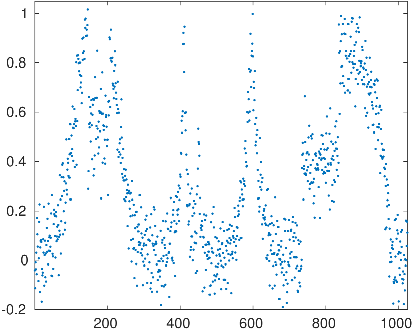
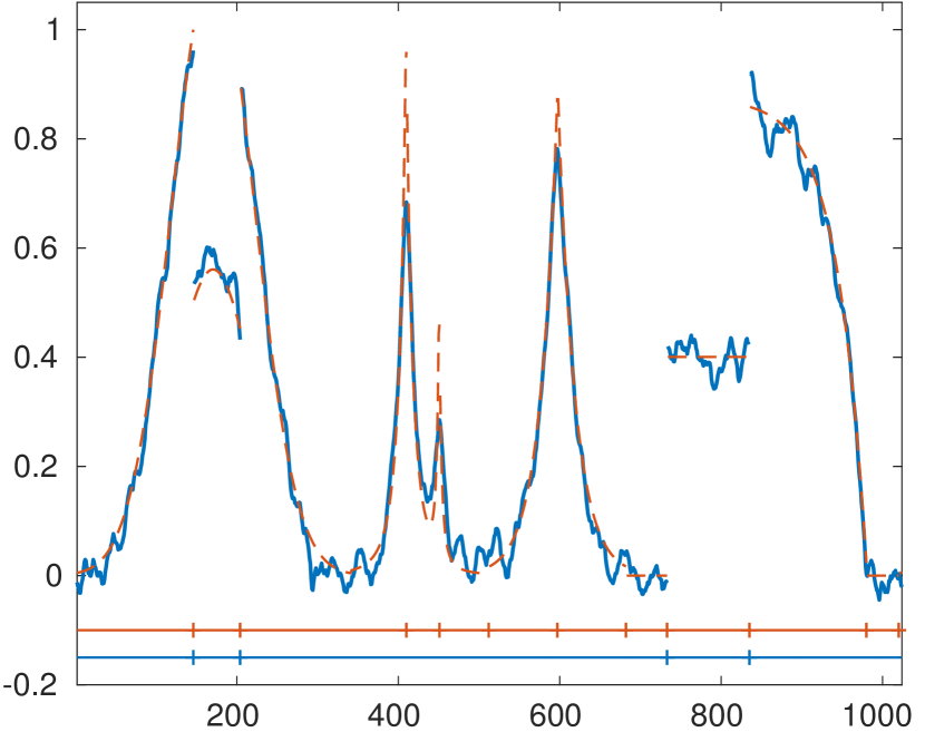
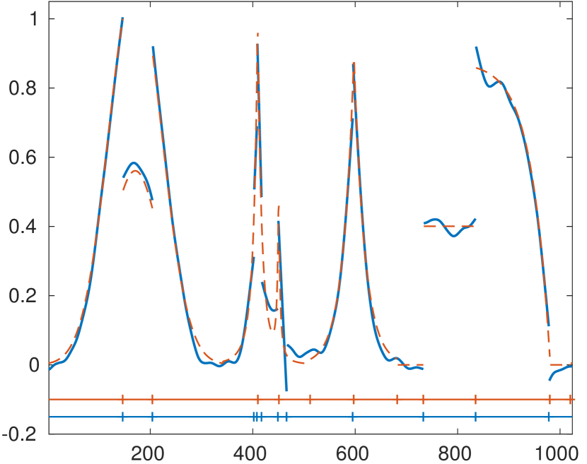
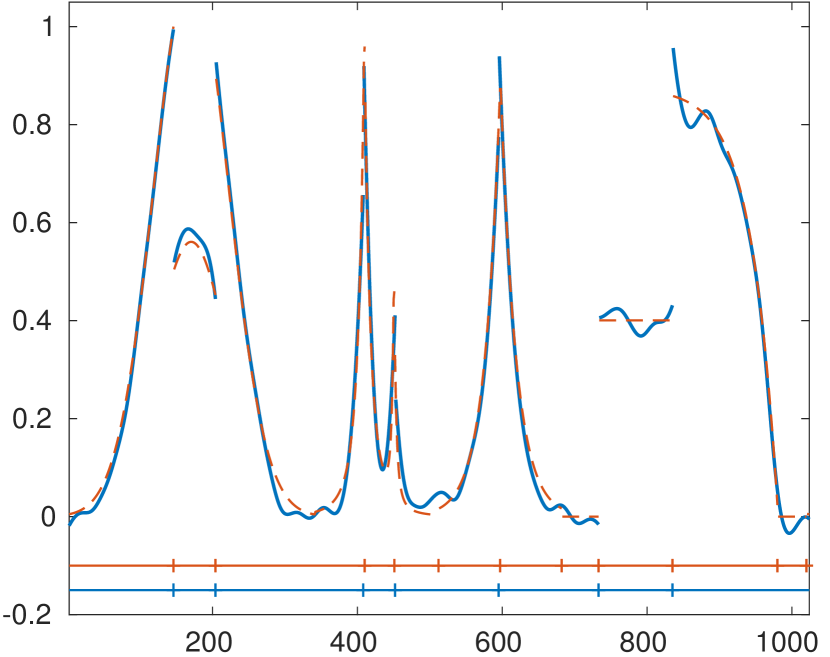
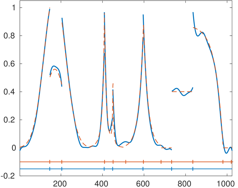
(c) $\eta=0.3$

Figure 7: Smoothing of piecewise defined signal of increasing noise level $\eta$ (top row). We observe that the segmentation quality gets higher and that the noise is smoothed out better on the segments when using higher order Mumford-Shah models.

We first investigate the potential of the higher order Mumford-Shah and Potts models with respect to reconstruction quality. We employ commonly used test signals with discontinuities; see [19, 45]. We corrupt the signals by additive zero mean Gaussian noise with variance $\sigma^{2}.$ We let the noise level $\eta$ be given by $\eta=\sigma N/\|g\|_{1},$ where $g$ denotes the clean signal. To obtain a meaningful comparison of the models’ potentials, we determined parameters $\beta$ and $\gamma$ such that the result $u^{*}$ has the best relative $\ell_{2}$-error $\varepsilon_{\text{rel}},$ given by $\varepsilon_{\text{rel}}=\|u^{*}-g\|_{2}/\|g\|_{2}.$ (We use a full grid search over $\gamma=(0,1]$ with stepsize $0.001,$ and $\beta\in(0,25]$ with stepsize $0.025$ and $\beta=\infty.$) We are further interested in the quality of the computed partition $\mathcal{I}^{*}.$ A commonly used measure for segmentation quality is the Rand index [52] which we briefly explain. The Rand index $\operatorname{R_{\text{ind}}}$ of two partitions $\mathcal{I},\mathcal{I}^{\prime}$ is given by $\operatorname{R_{\text{ind}}}(\mathcal{I},\mathcal{I}^{\prime})=\binom{N}{2}\sum_{\{i,j:\,1\leq i<j\leq N\}}t_{ij}$ where $t_{ij}$ is equal to one if there are $I\in\mathcal{I}$ and $I^{\prime}\in\mathcal{I}^{\prime}$ such that $i$ and $j$ are in both $I$ and $I^{\prime},$ or if $i$ is in both $I$ and $I^{\prime}$ while $j$ is in neither $I$ and $I^{\prime}.$ Otherwise, $t_{ij}=0.$ Further, $N$ denotes the length of the signal. The Rand index is bounded from above by one and a higher value means a better match. A value of one means that $\mathcal{I}$ and $\mathcal{I}^{\prime}$ agree. Here, we report the Rand index $\operatorname{R_{\text{ind}}}$ of the computed segmentation and the ground truth segmentation. It is worth recalling that a high parameter $\beta$ leads to stronger smoothing on the segments, and that a high parameter $\gamma$ leads to less segments.

The first signal is a sinusoidal with two steps (Figure 5). We observe that the first order model requires choosing a relatively small $\beta$ parameter to avoid the gradient limit effect. As tradeoff, the resulting signal remains visibly affected by the noise and the second discontinuity is smoothed out. Increasing the order $k$ to values greater than one leads to better results with respect to the segmentation quality. Furthermore, the relative error improves when increasing the order. The reconstruction quality starts decaying from order $k=6$ on which can be attributed to overfitting.

The second example is a piecewise constant signal (Figure 6). As the signal has no variation on the segments, the experiment confirms the intuition that large elasticity parameters – mostly $\beta=\infty$ – are preferable here. The best result is obtained by the first order Potts model as its search space is restricted to piecewise constant functions which perfectly matches the signal. Yet, using higher order models leads to very good segmentation results up to order $k=5$ and good reconstructions up to order $k=3,$ as well.

Figure 7 shows the reconstruction results for a piecewise smooth signal for different noise levels. We observe that the results of the first order model remain relatively noisy on the segments. A reason for this is that the elasticity parameter needs to be relatively small to prevent the gradient limit effect. Using the second order model improves the reconstruction results significantly but also tends to produce spurious segments, in particular at the parts of high curvature. Increasing the order to $k\geq 3,$ leads to better segmentations and improved smoothing on the segments.

An example of the effect of higher order Mumford-Shah on real data times series is given in Figure 8. The data are time-averaged (hourly) wind speeds at the summit of highest German mountain Zugspitze from November to December 2016. We observe that strong changes of the windspeed result in breakpoints of the higher order Mumford-Shah estimate. Some breakpoints can be associated with a meaning: the break at 492 and the two breaks near 1154 and 1182 can be linked with the days of strongest squalls in November and December 2016, respectively.

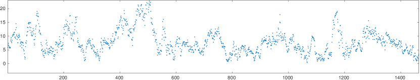
Figure 8: Top: Hourly averaged windspeeds [m/s] at the summit of the Zugspitze from November to December 2016. Bottom: Result of higher order Mumford-Shah model $(\mathcal{P}_{2;2;15}).$

4.2 Computation time

Time [s]	$k=$1	2	3	4
$n=$1000	0.0040	0.0049	0.0061	0.0065
4000	0.0183	0.0217	0.0268	0.0293
7000	0.0319	0.0382	0.0473	0.0513
10000	0.0464	0.0549	0.0682	0.0738

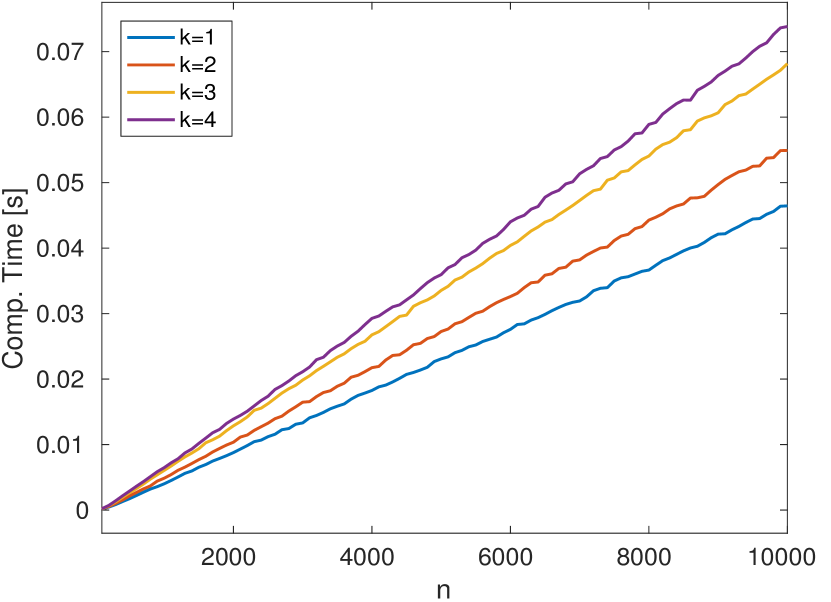
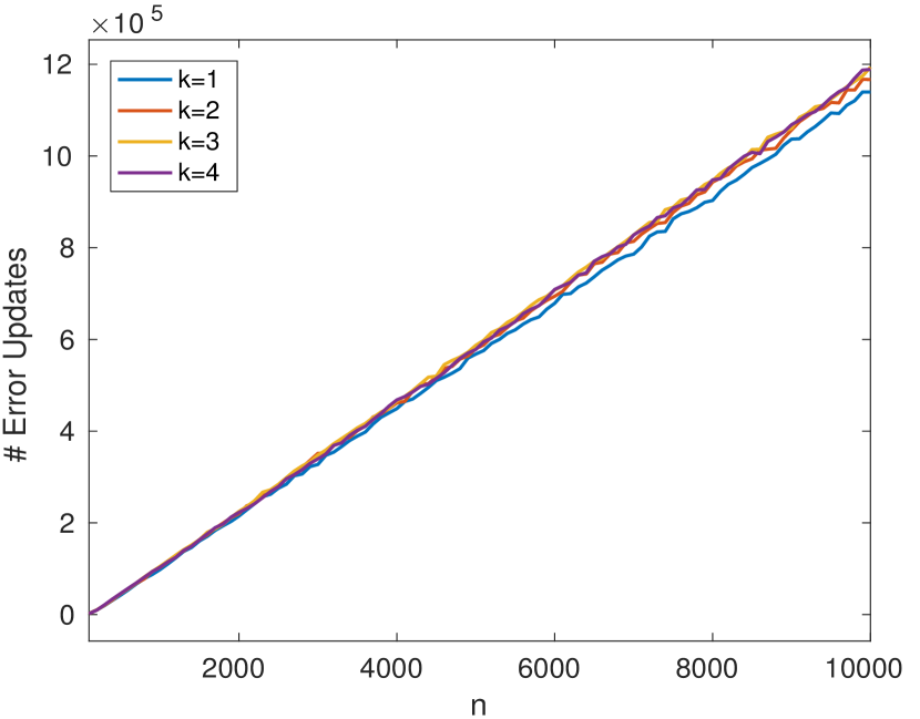
(a) Higher order Mumford-Shah model.

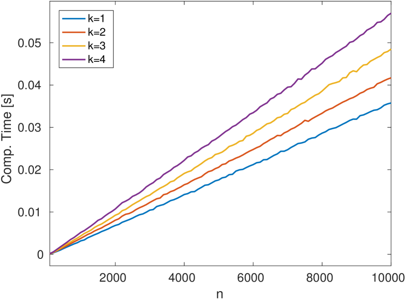
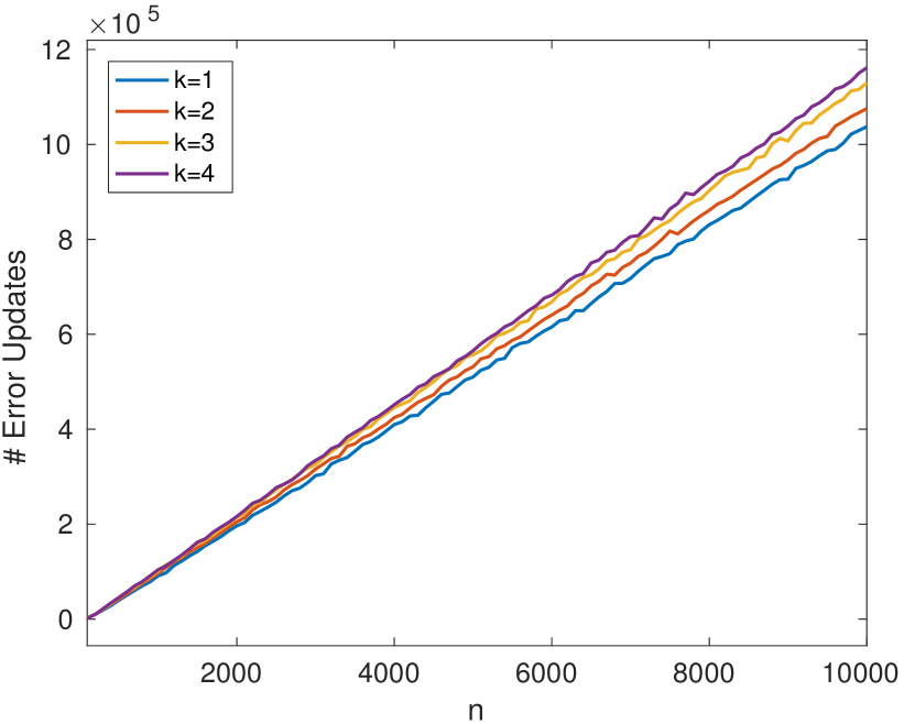
(b) Higher order Potts model.

(c) Computational costs of the proposed algorithm for the randomly generated piecewise polynomial signals corrupted by Gaussian noise of level $\eta=0.1.$ Computation times for selected lengths $N$ are tabulated (top) and plotted for $N=100,200,\ldots,10000$ (center). We observe that the runtime only grows linearly in $N,$ so much more favorable than the worst case scenario of quadratic growth. This means that the pruning strategies show their full effectiveness for this type of signals, which is reflected by the linear growth in the number of error updates (bottom).

We investigate the computation time and the number of executed error updates depending on the signal length $N.$ To this end, we generate two types of synthetic signals: signals with increasing number of discontinuities and signals with constant number of discontinuities.

The signals are generated as follows. For the first type we let for each $g_{i},i=1,\ldots,N,$ the probability of a jump discontinuity be $p=0.01$; that is, the length of each smooth segment $I$ of $g$ follows a geometric distribution with parameter $p$. Hence, the expected segment length is $1/p=100,$ and the expected number of segments grows linearly with respect to $N$. Within a segment $I$ the signal $g$ is polynomial of degree $k-1$ with coefficients generated by the random variables $\frac{1}{(j+1)^{2}}X_{j}$, $j=1,...,k$, where $X_{j}$ are i.i.d. uniformly distributed on $[-1,1]$. For the length $h$ of $I$, the domain of $g_{I}$ is $[0,hp]$ sampled with step size $p$. For spline order $k$, the degree of polynomials is set to $k-1$. The second type of signals is created by taking $N$ equidistant samples of the continuously defined signal shown in Figure 7. In all cases, the signals are corrupted by additive Gaussian noise with noise level $\eta=0.1$. For every considered $N$, we computed $1000$ realizations and report the mean computation time and the mean number of performed error updates, respectively.

The results for the first type of signals are shown in Section 4.2. It is an important observation that the runtime and the errors updates exhibit linear growth in the signal length. Thus, the proposed algorithm does not show its worst case complexity. That means, that the utilized pruning strategies are highly effective. The results for the second type of signals are shown in Section 4.2. In contrast to the first type, the computation time grows approximately quadratic in the number of elements, which means that the proposed algorithm attains its worst case complexity. These results suggest that an increasing number of discontinuities is beneficial for the efficiency of the proposed algorithm.

(d) Runtime [s] for (higher order) Mumford-Shah solver

(e) Runtime [s] for (higher order) Potts solver

(f) Mean computation times of the proposed algorithm (in seconds) for the signal from Figure 7 sampled on $N$ points and corrupted by Gaussian noise with noise level $0.1.$ We observe that the runtime grows approximately quadratic in $N$; that is, the worst case complexity is attained. The relevant difference to the experiment in Section 4.2 is that the number of discontinuities does not increase with $N.$ Yet, the solver processes signals of size $2^{16}$ in less than one minute.

5 Conclusion

We have studied higher order Mumford-Shah and Potts models. Their central advantage compared with classical first order models is that they do not penalize polynomial trends of order $k-1$ on the segments. This leads to improved estimation for data with piecewise linear or polynomial trends. We have shown that the defining functionals have unique minimizers for almost all input signals. We have proposed a fast solver for higher order Mumford-Shah and Potts models. We have obtain stability results. We have shown that the worst case complexity of the proposed algorithm is quadratic in the length of the signal for arbitrary orders $k\geq 1.$ In the numerical experiments, we have further observed that the runtime grows only linear for signals with linearly increasing number of discontinuities. Further, the numerical experiments confirm the robustness and stability of the proposed method. Our reference implementation processes even long signals in reasonable time; for example signals of length $10,000$ need less than one second. This way, the family of higher order Mumford-Shah and Potts models can serve as efficient smoothers for signals with discontinuities.

Acknowledgement

This work was supported by the German Research Foundation (DFG grants STO1126/2-1 and WE5886/4-1).

Appendix A Pseudocode of the proposed solver

A pseudocode for the proposed solver for ($\mathcal{P}_{k,\beta,\gamma}$) is given in Algorithm 1.

Input: Data $f\in\mathbb{R}^{N}$; model parameters $k\in\mathbb{N},\beta\in(0,\infty],\gamma>0;$

Output: Global minimizer $(u^{*},\mathcal{I}^{*})$ of ($\mathcal{P}_{k,\beta,\gamma}$) or ($\mathcal{P}_{k,\infty,\gamma}$)

/* Precomputations */

1 Row-wise transform the matrix $\quad\begin{cases}\eqref{eq:penalizedProblem}:&\text{ $A$ from \eqref{eq:AmatrixGvector}}\\ \eqref{eq:penalizedProblemPoly}:&\text{ $B$ from \eqref{eq:systemMatrixPoly}}\end{cases}$
to upper triangular form using successive Givens rotations and store the rotation angles in $\Theta$.

2Compute $\mathcal{E}^{{1:r}}$ for all $r=1,\ldots,N$ with $\Theta$

/* Find optimal changepoints */

3 Initialize lists $L=[2]$, $R=[2]$, $E=[0]$

4 $J_{1}\leftarrow 0$, $P^{*}_{1}\leftarrow 0$

5 for $r\leftarrow 2,\ldots,N$ do

       /* Initialization */

6       $J_{r}\leftarrow 0$, $P_{r}^{*}\leftarrow\mathcal{E}^{{1:r}}$

       /* Find optimal $P_{r}^{*}$ using (25) */

7       for $i=1,...,\text{length of }L$ do

8             while $r_{i}<r$ do

                   /* Update approximation error */

9                   $\begin{cases}\eqref{eq:penalizedProblem}:\text{ Compute $\mathcal{E}^{l_{i}:r_{i}+1}$ from $\mathcal{E}^{l_{i}:r_{i}}$ using the recurrence \eqref{eq:recurrence_q}-\eqref{eq:ErrorUpdate_new} }\\ \eqref{eq:penalizedProblemPoly}:\text{ Compute $\mathcal{E}^{l_{i}:r_{i}+1}$ from $\mathcal{E}^{l_{i}:r_{i}}$ using the recurrence \eqref{eq:recurrence_q_Potts}-\eqref{eq:ErrorUpdatePoly} }\end{cases}$ 

10                   $E_{i}\leftarrow\mathcal{E}^{{l_{i}:r_{i}+1}}$,

11                   $r_{i}\leftarrow r_{i}+1$

                   /* Pruning (27) */

12                   if $P^{*}_{l_{i}-1}+E_{i}\geq P_{r_{i}}^{*}$ then

13                         Delete: $l_{i}$ from $L$, $r_{i}$ from $R$ and $E_{i}$ from $E$

14                         go to 1

15                   end if

16                  

17             end while

18            $b\leftarrow P^{*}_{l_{i}-1}+\gamma+E_{i}$

19             if $b\leq P_{r}^{*}$ then

20                   $P_{r}^{*}\leftarrow b$, $J_{r}\leftarrow l-1$

21             end if

            /* Pruning (26) */

22             If $E_{i}+\gamma>P^{*}_{r}$ then break end

23       end for

      /* Update lists */

24       Prepend: $r+1$ to $L$, $r+1$ to $R$, $0$ to $E$

25 end for

/* Recover partition $\mathcal{I}^{*}$ from segment boundary locations $J$ */

26 $r\leftarrow N$, $\mathcal{I}^{*}\leftarrow\emptyset$

27 while $r>0$ do

28       $l\leftarrow J(r)+1$, $\mathcal{I}^{*}\leftarrow\mathcal{I}^{*}\cup\{(l:r)\}$, $r\leftarrow l-1$

29 end while

/* Reconstruction of $u^{*}$ by solving linear systems on segments (using QR decomposition and reusing $\Theta$ for speedup) */

30 for $I\in\mathcal{I^{*}}$ do

31       $\begin{cases}\text{ \eqref{eq:penalizedProblem}: Solve $u_{I}^{*}=\operatorname*{argmin}\limits_{v\in\mathbb{R}^{|I|}}\|v-f_{I}\|_{2}^{2}+\beta^{2k}\|\nabla^{k}v\|_{2}^{2}$ }\\ \text{ \eqref{eq:penalizedProblemPoly}: Solve $u_{I}^{*}=\operatorname*{argmin}\|v-f_{I}\|_{2}^{2}$ such that $v$ is polynomial of degree $\leq k-1$ on $I$ }\end{cases}$

32 end for

Algorithm 1 Solver for the higher order Mumford-Shah problem and higher order Potts problem

References

- Amat et al. [2017] S. Amat, Z. Li, and J. Ruiz. On an new algorithm for function approximation with full accuracy in the presence of discontinuities based on the immersed interface method. Journal of Scientific Computing, pages 1–35, 2017.
- Ambrosio and Tortorelli [1990] L. Ambrosio and V. M. Tortorelli. Approximation of functional depending on jumps by elliptic functional via -convergence. Communications on Pure and Applied Mathematics, 43(8):999–1036, 1990.
- Arandiga et al. [2005] F. Arandiga, A. Cohen, R. Donat, and N. Dyn. Interpolation and approximation of piecewise smooth functions. SIAM Journal on Numerical Analysis, 43(1):41–57, 2005.
- Artina et al. [2013] M. Artina, M. Fornasier, and F. Solombrino. Linearly constrained nonsmooth and nonconvex minimization. SIAM Journal on Optimization, 23(3):1904–1937, 2013.
- Auger and Lawrence [1989] I. Auger and C. Lawrence. Algorithms for the optimal identification of segment neighborhoods. Bulletin of Mathematical Biology, 51(1):39–54, 1989.
- Bar et al. [2004] L. Bar, N. Sochen, and N. Kiryati. Variational pairing of image segmentation and blind restoration. In ECCV, pages 166–177. Springer, 2004.
- Bellman and Roth [1969] R. Bellman and R. Roth. Curve fitting by segmented straight lines. Journal of the American Statistical Association, 64(327):1079–1084, 1969.
- Blake and Zisserman [1987] A. Blake and A. Zisserman. Visual reconstruction. MIT Press Cambridge, 1987.
- Blake [1989] A. Blake. Comparison of the efficiency of deterministic and stochastic algorithms for visual reconstruction. IEEE Transactions on Pattern Analysis and Machine Intelligence, 11(1):2–12, 1989.
- Boykov et al. [2001] Y. Boykov, O. Veksler, and R. Zabih. Fast approximate energy minimization via graph cuts. IEEE Transactions on Pattern Analysis and Machine Intelligence, 23(11):1222–1239, 2001.
- Bredies et al. [2010] K. Bredies, K. Kunisch, and T. Pock. Total generalized variation. SIAM Journal on Imaging Sciences, 3(3):492–526, 2010.
- Bruce [1965] J. Bruce. Optimum quantization. Technical report, Massachusetts Institute of Technology, 1965.
- Carriero et al. [2015] M. Carriero, A. Leaci, and F. Tomarelli. A survey on the Blake–Zisserman functional. Milan Journal of Mathematics, 83(2):397–420, 2015.
- Chambolle [1995] A. Chambolle. Image segmentation by variational methods: Mumford and Shah functional and the discrete approximations. SIAM Journal on Applied Mathematics, 55(3):827–863, 1995.
- Chambolle [1999] A. Chambolle. Finite-differences discretizations of the Mumford-Shah functional. ESAIM: Mathematical Modelling and Numerical Analysis, 33(02):261–288, 1999.
- Chambolle and Lions [1997] A. Chambolle and P.-L. Lions. Image recovery via total variation minimization and related problems. Numerische Mathematik, 76(2):167–188, 1997.
- Chan and Vese [2001] T. Chan and L. Vese. Active contours without edges. IEEE Transactions on Image Processing, 10(2):266–277, 2001.
- Chen et al. [2017] C. Chen, J. Leng, and G. Xu. A general framework of piecewise-polynomial Mumford-Shah model for image segmentation. International Journal of Computer Mathematics, 94(10):1981–1997, 2017.
- Donoho and Johnstone [1994] D. Donoho and I. Johnstone. Ideal spatial adaptation by wavelet shrinkage. Biometrika, pages 425–455, 1994.
- Drobyshev et al. [2003] A. Drobyshev, C. Machka, M. Horsch, M. Seltmann, V. Liebscher, M. de Angelis, and J. Beckers. Specificity assessment from fractionation experiments (safe): a novel method to evaluate microarray probe specificity based on hybridisation stringencies. Nucleic acids research, 31(2):1–10, 2003.
- Fearnhead et al. [2018] P. Fearnhead, R. Maidstone, and A. Letchford. Detecting changes in slope with an l0 penalty. Journal of Computational and Graphical Statistics, 0(0):1–11, 2018.
- Fornasier and Ward [2010] M. Fornasier and R. Ward. Iterative thresholding meets free-discontinuity problems. Foundations of Computational Mathematics, 10(5):527–567, 2010.
- Fornasier et al. [2013] M. Fornasier, R. March, and F. Solombrino. Existence of minimizers of the mumford-shah functional with singular operators and unbounded data. Annali di Matematica Pura ed Applicata, 192(3):361–391, 2013.
- Fortun et al. [2018] D. Fortun, M. Storath, D. Rickert, A. Weinmann, and M. Unser. Fast piecewise-affine motion estimation without segmentation. IEEE Transactions on Image Processing, 27(11):5612–5624, Nov 2018.
- Frick et al. [2014] K. Frick, A. Munk, and H. Sieling. Multiscale change point inference. Journal of the Royal Statistical Society: Series B (Statistical Methodology), 76(3):495–580, 2014.
- Friedrich et al. [2008] F. Friedrich, A. Kempe, V. Liebscher, and G. Winkler. Complexity penalized M-estimation: Fast computation. Journal of Computational and Graphical Statistics, 17(1):201–224, 2008.
- Geman and Geman [1984] S. Geman and D. Geman. Stochastic relaxation, Gibbs distributions, and the Bayesian restoration of images. IEEE Transactions on Pattern Analysis and Machine Intelligence, 6(6):721–741, 1984.
- Gentleman [1973] W. Gentleman. Least squares computations by Givens transformations without square roots. J. Inst. Maths Applies, 12:329–336, 1973.
- Harten [1996] A. Harten. Multiresolution representation of data: A general framework. SIAM Journal on Numerical Analysis, 33(3):1205–1256, 1996.
- Hohm et al. [2015] K. Hohm, M. Storath, and A. Weinmann. An algorithmic framework for Mumford-Shah regularization of inverse problems in imaging. Inverse Problems, 31(11):115011, 2015.
- Hotz et al. [2013] T. Hotz, O. M. Schutte, H. Sieling, T. Polupanow, U. Diederichsen, C. Steinem, and A. Munk. Idealizing ion channel recordings by a jump segmentation multiresolution filter. IEEE Transactions on NanoBioscience, 12(4):376–386, 2013.
- Hupé et al. [2004] P. Hupé, N. Stransky, J. Thiery, F. Radvanyi, and E. Barillot. Analysis of array CGH data: from signal ratio to gain and loss of DNA regions. Bioinformatics, 20(18):3413–3422, 2004.
- Isack et al. [2016] H. Isack, O. Veksler, M. Sonka, and Y. Boykov. Hedgehog shape priors for multi-object segmentation. In Proceedings of the IEEE Conference on Computer Vision and Pattern Recognition, pages 2434–2442, 2016.
- Jackson et al. [2005] B. Jackson, J. D. Scargle, D. Barnes, S. Arabhi, A. Alt, P. Gioumousis, E. Gwin, P. Sangtrakulcharoen, L. Tan, and T. Tsai. An algorithm for optimal partitioning of data on an interval. IEEE Signal Processing Letters, 12(2):105–108, 2005.
- Jiang et al. [2014] M. Jiang, P. Maass, and T. Page. Regularizing properties of the Mumford-Shah functional for imaging applications. Inverse Problems, 30(3):035007, 2014.
- Joo et al. [2008] C. Joo, H. Balci, Y. Ishitsuka, C. Buranachai, and T. Ha. Advances in single-molecule fluorescence methods for molecular biology. Annual Review of Biochemistry, 77:51–76, 2008.
- Kiefer et al. [2018] L. Kiefer, M. Storath, and A. Weinmann. Iterative Potts minimization for the recovery of signals with discontinuities from indirect measurements – the multivariate case. arXiv:1812.00862, 2018.
- Killick et al. [2012] R. Killick, P. Fearnhead, and I. Eckley. Optimal detection of changepoints with a linear computational cost. Journal of the American Statistical Association, 107(500):1590–1598, 2012.
- Kleinberg and Tardos [2006] J. Kleinberg and E. Tardos. Algorithm design. Pearson Education India, 2006.
- Kolmogorov et al. [2015] V. Kolmogorov, T. Pock, and M. Rolinek. Total variation on a tree. Preprint arXiv:1502.07770, 2015.
- Lemire [2007] D. Lemire. A better alternative to piecewise linear time series segmentation. In Proceedings of the 2007 SIAM International Conference on Data Mining, pages 545–550. SIAM, 2007.
- Liebscher and Winkler [1999] V. Liebscher and G. Winkler. A potts model for segmentation and jump-detection. In Proceedings S4G International Conference on Stereology, Spatial Statistics and Stochastic Geometry, Prague June, volume 21, pages 185–190. Citeseer, 1999.
- Little and Jones [2011a] M. Little and N. Jones. Generalized methods and solvers for noise removal from piecewise constant signals. I. Background theory. Proceedings of the Royal Society A: Mathematical, Physical and Engineering Science, 467(2135):3088–3114, 2011a.
- Little and Jones [2011b] M. Little and N. Jones. Generalized methods and solvers for noise removal from piecewise constant signals. II. New methods. Proceedings of the Royal Society A: Mathematical, Physical and Engineering Science, 467(2135):3115–3140, 2011b.
- Mallat [2008] S. Mallat. A wavelet tour of signal processing: the sparse way. Academic press, 2008.
- Mumford and Shah [1985] D. Mumford and J. Shah. Boundary detection by minimizing functionals. In IEEE Conference on Computer Vision and Pattern Recognition, volume 17, pages 137–154, 1985.
- Mumford and Shah [1989] D. Mumford and J. Shah. Optimal approximations by piecewise smooth functions and associated variational problems. Communications on Pure and Applied Mathematics, 42(5):577–685, 1989.
- Nord et al. [2017] A. L. Nord, E. Gachon, R. Perez-Carrasco, J. A. Nirody, A. Barducci, R. M. Berry, and F. Pedaci. Catch bond drives stator mechanosensitivity in the bacterial flagellar motor. Proceedings of the National Academy of Sciences, 114(49):12952–12957, 2017.
- Potts [1952] R. Potts. Some generalized order-disorder transformations. Mathematical Proceedings of the Cambridge Philosophical Society, 48(1):106–109, 1952.
- Ramlau and Ring [2007] R. Ramlau and W. Ring. A mumford–shah level-set approach for the inversion and segmentation of x-ray tomography data. Journal of Computational Physics, 221(2):539–557, 2007.
- Ramlau and Ring [2010] R. Ramlau and W. Ring. Regularization of ill-posed mumford–shah models with perimeter penalization. Inverse Problems, 26(11):115001, 2010.
- Rand [1971] W. Rand. Objective criteria for the evaluation of clustering methods. Journal of the American Statistical Association, 66(336):846, dec 1971.
- Rondi [2008] L. Rondi. On the regularization of the inverse conductivity problem with discontinuous conductivities. Inverse Problems & Imaging, 2(3):397–409, 2008.
- Rondi and Santosa [2001] L. Rondi and F. Santosa. Enhanced electrical impedance tomography via the mumford–shah functional. ESAIM: Control, Optimisation and Calculus of Variations, 6:517–538, 2001.
- Rudin et al. [1992] L. Rudin, S. Osher, and E. Fatemi. Nonlinear total variation based noise removal algorithms. Physica D: Nonlinear Phenomena, 60(1):259–268, 1992.
- Snijders et al. [2001] A. Snijders, N. Nowak, R. Segraves, et al. Assembly of microarrays for genome-wide measurement of DNA copy number by CGH. Nature Genetics, 29:263–264, 2001.
- Sowa et al. [2005] Y. Sowa, A. Rowe, M. Leake, T. Yakushi, M. Homma, A. Ishijima, and R. Berry. Direct observation of steps in rotation of the bacterial flagellar motor. Nature, 437(7060):916–919, 2005.
- Storath et al. [2017] M. Storath, A. Weinmann, and M. Unser. Jump-penalized least absolute values estimation of scalar or circle-valued signals. Information and Inference, 6(3):225–245, 2017.
- Storath and Weinmann [2014] M. Storath and A. Weinmann. Fast partitioning of vector-valued images. SIAM Journal on Imaging Sciences, 7(3):1826–1852, 2014.
- Strekalovskiy et al. [2012] E. Strekalovskiy, A. Chambolle, and D. Cremers. A convex representation for the vectorial Mumford-Shah functional. In IEEE Conference on Computer Vision and Pattern Recognition (CVPR), pages 1712–1719, 2012.
- Strekalovskiy and Cremers [2014] E. Strekalovskiy and D. Cremers. Real-time minimization of the piecewise smooth Mumford-Shah functional. In European Conference on Computer Vision, pages 127–141. Springer, 2014.
- Tsai et al. [2001] A. Tsai, A. Yezzi, and A. S. Willsky. Curve evolution implementation of the mumford-shah functional for image segmentation, denoising, interpolation, and magnification. IEEE transactions on Image Processing, 10(8):1169–1186, 2001.
- Veksler [1999] O. Veksler. Efficient graph-based energy minimization methods in computer vision. PhD thesis, Cornell University, 1999.
- Wahba [1990] G. Wahba. Spline models for observational data. SIAM, 1990.
- Wang et al. [2013] Y. Wang, S. Xiang, C. Pan, L. Wang, and G. Meng. Level set evolution with locally linear classification for image segmentation. Pattern Recognition, 46(6):1734–1746, 2013.
- Wang and Vemuri [2005] Z. Wang and B. C. Vemuri. Dti segmentation using an information theoretic tensor dissimilarity measure. IEEE transactions on medical imaging, 24(10):1267–1277, 2005.
- Weinmann and Storath [2015] A. Weinmann and M. Storath. Iterative Potts and Blake-Zisserman minimization for the recovery of functions with discontinuities from indirect measurements. Proceedings of the Royal Society A, 471(2176), 2015.
- Weinmann et al. [2015] A. Weinmann, M. Storath, and L. Demaret. The -Potts functional for robust jump-sparse reconstruction. SIAM Journal on Numerical Analysis, 53(1):644–673, 2015.
- Weinmann et al. [2016] A. Weinmann, L. Demaret, and M. Storath. Mumford-Shah and Potts regularization for manifold-valued data. Journal of Mathematical Imaging and Vision, 55(3):428–445, 2016.
- Whittaker [1922] E. Whittaker. On a new method of graduation. Proceedings of the Edinburgh Mathematical Society, 41:63–75, 1922.
- Wilkinson [1965] J. Wilkinson. The algebraic eigenvalue problem. Monographs on numerical analysis. Clarendon Press, Oxford, 1965.
- Winkler [2003] G. Winkler. Image analysis, random fields and Markov chain Monte Carlo methods: a mathematical introduction, volume 27. Springer Verlag, 2003.
- Winkler and Liebscher [2002] G. Winkler and V. Liebscher. Smoothers for discontinuous signals. Journal of Nonparametric Statistics, 14(1-2):203–222, 2002.
- Winkler et al. [2005] G. Winkler, O. Wittich, V. Liebscher, and A. Kempe. Don’t shed tears over breaks. Jahresbericht der Deutschen Mathematiker-Vereinigung, 107:57–87, 2005.
- Wittich et al. [2008] O. Wittich, A. Kempe, G. Winkler, and V. Liebscher. Complexity penalized least squares estimators: Analytical results. Mathematische Nachrichten, 281(4):582–595, 2008.
- Yang and Li [2015] J. Yang and H. Li. Dense, accurate optical flow estimation with piecewise parametric model. In Proceedings of the IEEE Conference on Computer Vision and Pattern Recognition, pages 1019–1027, 2015.
- Zanetti and Bruzzone [2017] M. Zanetti and L. Bruzzone. Piecewise linear approximation of vector-valued images and curves via second-order variational model. IEEE Transactions on Image Processing, 26(9):4414–4429, 2017.
- Zanetti et al. [2016] M. Zanetti, V. Ruggiero, and M. Miranda Jr. Numerical minimization of a second-order functional for image segmentation. Communications in nonlinear science and numerical simulation, 36:528–548, 2016.